HIDDEN MARKOV RANDOM FIELDS AND CUCKOO SEARCH METHOD FOR MEDICAL IMAGE SEGMENTATION

Abstract

Segmentation of medical images is an essential part in the process of diagnostics. Physicians require an automatic, robust and valid results. Hidden Markov Random Fields (HMRF) provide powerful model. This latter models the segmentation problem as the minimization of an energy function. Cuckoo search (CS) algorithm is one of the recent nature-inspired meta-heuristic algorithms. It has shown its efficiency in many engineering optimization problems. In this paper, we use three cuckoo search algorithm to achieve medical image segmentation.

Index Terms—  Brain image segmentation; Hidden Markov Random Field; Cuckoo Search algorithm; Dice Coefficient metric.

1 INTRODUCTION

With the overwhelming number of medical images, the manual analysis and interpretation of images from different imaging modalities (Radiography, Magnetic Resonance Imaging (MRI), Computed Tomography (CT), etc ) became a tedious task. This fact underlines the necessity of automatic image analysis, through several operations including segmentation.

Segmentation is the process of partitioning an image into multiple segments semantically interpretable. For MRI, segmentation is hard because MR images are usually corrupted by noise and non-uniformity artifact due to various factors, such as partial variations in illumination or radio frequency coil in image acquisition devices.

In this work, we use Hidden Markov random field (HMRF) model [1, 2, 3] for image segmentation: the hidden information, namely the segmented image, is computed from the original image by maximizing the MAP criterion (Maximum A Posterior). Since the objective function of the MAP is non-linear, complex and may have several local maxima, meta-heuristic algorithms are preferred for optimization.

The use of meta-heuristic algorithms for image segmentation is not new. Several methods have been proposed in the literature, for instance, the cuckoo search (CS) algorithm. It is one of the latest nature-inspired meta-heuristic algorithms, it was proposed in 2009 by Xin-She Yang and Suash Deb [4]. CS is based on the brood parasitism of some cuckoo species. In addition, this algorithm is enhanced by the so-called Lévy flights rather than by simple isotropic random walks.

In this paper, we compare three variants of cuckoo search (standard CS [4, 5, 6], improved CS [7] and auto adaptative modified CS [8]) to optimize the HMRF model for MRI segmentation. In this specific case, the segmentation consists in partitioning the brain image into different parts that are: gray matter(GM), white matter (WM) and cerebrospinal fluid (CSF). The quality evaluation is conducted on ground-truth images from BrainWeb and IBSR databases, using the Dice coefficient metric [9].

The rest of the paper is organized as follows. In Part II, the HMRF model principles in the context of image segmentation is described. The combination of HMRF and cuckoo search algorithm is explained in Part III. Finally, in Part IV and Part V, experimental results on medical image samples are illustrated and conclusions are drawn, respectively.

2 HIDDEN MARKOV RANDOM FIELD MODEL

Let $y=({y}_{1},{y}_{2},{\dots},{y}_{M})$ be the image to segment into $K$ classes and $x=({x}_{1},{x}_{2},{\dots},{x}_{M})$ be the segmented image. $y_{s}$ is pixel value of the site $s$ that takes its values in the gray level space $E_{y}=\{0,\ldots,255\}$. $x_{s}$ is class of the site $s$ and takes its values in the discrete space $E_{x}=\left\{1,{\dots},K\right\}$.

The image to segment $y$ and the segmented image $x$ represent respectively realizations of Markov Random Fields $Y=({Y}_{1},{Y}_{2},{\dots},{Y}_{M})$ and $X=({X}_{1},{X}_{2},{\dots},{X}_{M})$. Configurations set of the image to segment $y$ and of the segmented image are respectively $\Omega_{y}=E_{y}^{M}$ and $\Omega_{x}=E_{x}^{M}$.

Let $\mu=(\mu_{1},\dots,\mu_{j},\dots,\mu_{K})$ be the means and $\sigma=(\sigma_{1},\dots,\sigma_{j},\dots,\sigma_{K})$ be the standard deviations of the $K$ classes in the segmented image $x=(x_{1},\dots,x_{s},\dots,x_{M})$ i.e.,

$${}\begin{array}[]{l}\begin{cases}\mu_{j}={\frac{1}{|S_{j}|}\sum_{s\in S_{j}}y_{s}}\\ \sigma_{j}=\sqrt{\frac{1}{|S_{j}|}\sum_{s\in S_{j}}(y_{s}-\mu_{j})^{2}}\\ S_{j}=\{s\ |\ x_{s}=j\}\end{cases}\end{array}$$ (1)

Hidden Markov Random Field approach is modelled in [10] as a minimization of the function $\Psi(\mu)$ defined below. We can always compute $x$ through $\mu$ by classifying $y_{s}$ into the nearest mean $\mu_{j}$ i.e., $x_{s}=j$ if the nearest mean to $y_{s}$ is $\mu_{j}$. Thus, we look for $\mu^{*}$. The configuration set of $\mu$ is $\Omega_{\mu}=[0\dots 255]^{K}$.

$$\begin{array}[]{l}\begin{cases}{\mu}^{*}=\operatorname*{arg}_{\mu\in\Omega_{\mu}}{\mathit{\min}}\left\{\Psi(\mu)\right\}\\ \\ \Psi(\mu)=\sum_{j=1}^{K}f(\mu_{j})\\ \\ f(\mu_{j})=\sum\limits_{s\in S_{j}}{[\ln(\sigma_{j})+\frac{(y_{s}-\mu_{j})^{2}}{2\sigma_{j}^{2}}]}\\ \quad\quad\quad\quad+\frac{B}{T}\sum_{c_{2}=\{s,t\}}{(1-2\delta(x_{s},x_{t}))}\end{cases}\end{array}$$ (2)

where $B$ is a constant, $T$ is a control parameter called temperature, $\delta$ is Kronecker’s delta and $S_{j}$, $\mu_{j}$ and $\sigma_{j}$ are defined in (1). When $B>0$, the most likely segmentation corresponds to the constitution of large homogeneous regions. The size of these regions is controlled by the parameter $B$.

To apply unconstrained optimization techniques, we redefine the function $\Psi(\mu)$ for $\mu\in\mathbb{R}^{K}$ instead of $\mu\in[0\dots 255]^{K}$ as recommended by [11]. Therefore, the new function $\Psi(\mu)$ becomes as follows:

$$\Psi(\mu)=\sum_{j=1}^{K}F(\mu_{j})\ \ \mbox{where }\mu_{j}\in\mathbb{R}$$ (3)

$$F(\mu_{j})=\begin{cases}f(0)-u_{j}*10^{3}&\mbox{if }\mu_{j}<0\\ f(\mu_{j})&\mbox{if }\mu_{j}\in[0\dots 255]\\ f(255)+(u_{j}-255)*10^{3}&\mbox{if }\mu_{j}>255\end{cases}$$

3 Hidden Markov Random Field and Cuckoo Search (CS) algorithm

To solve the minimization problem expressed in the 3, we used Cuckoo Search (CS) algorithm. The principal steps are set out below.

Each egg in a host nest represents a solution $\mu^{i,t}=(\mu^{i,t}_{1},\dots,\mu^{i,t}_{j},\dots,\mu^{i,t}_{K})$ at time $t$.

Let $c^{i,t}=(c^{i,t}_{1},,\dots,c^{i,t}_{j},\dots,c^{i,t}_{K})$ be cuckoo egg generated at time $t$.

Let $n$ be the number of available host nests (or different solutions). The initial population $\{\mu^{i,0}\}_{i=1,\dots,n}$ is generated by random initialization.

Let $\mbox{best}^{t}=(\mbox{best}^{t}_{1},\dots,\mbox{best}^{t}_{j},\dots,\mbox{best}^{t}_{K})$ be the best solution at time $t$.

$$\mbox{best}^{t}:=\arg\min\limits_{\mu^{i,t}_{i=0,\dots,n}}{\Psi(\mu^{i,t})}$$ (4)

Cuckoo Search (CS) algorithm is based on three rules defined in [4, 5] and proceeds as follows:

1. Generating new cuckoos $\{c^{i,t}\}_{i=1,\dots,n}$ can be performed as follows (Lévy flight):

   $$c^{i,t}:=\mu^{i,t}+\alpha\times\mbox{\mbox{step}}\otimes(\mu^{i,t}-\mbox{best}^{t})\otimes randn(1,K)$$ (5)

   where $\otimes$ means the entry-wise product of two vectors. The $randn(1,K)$ returns $K$ random numbers from a normal distribution with mean 0 and variance 1.

   Here $\alpha>0$ is the step size scaling factor, which should be related to the scales of the problem of interest.

   step is used in the application of Lévy flights, see in [6] for more detail. For standard random walks, use $\mbox{step}=1$.

2. After generating new cuckoos, we update nests $\mu^{i,t}$ as follows:

   $$\mu^{i,t}:=\begin{cases}c^{i,t}&\mbox{if }\Psi(c^{i,t})\leq\Psi(\mu^{i,t})\\ \mu^{i,t}&\mbox{otherwise}\end{cases}$$ (6)

3. A fraction of worse nests are discovered with a probability $p_{a}$. For that, we construct new solutions $\mu^{i,t+1}$ as follows (biased/selective random walks):

   $$\mu^{i,t+1}:=\mu^{i,t}+[rand()]\otimes[H(p_{a}-rand())]\otimes(\mu^{a,t}-\mu^{b,t})$$ (7)

   where $\mu^{a,t}$ and $\mu^{b,t}$ are two different solutions selected randomly by random permutation. $H$ is Heaviside function. $rand()$ returns a single uniformly distributed random number in the interval (0,1). $[\ ]$ is a $K$ vector.

Each variant of CS manages in a specific way $p_{a}$, $\alpha$ and step.

The HMRF-CS combination is summarized in Algorithm 1.

Objective function $\Psi(\mu),\mu=(\mu_{1},...,\mu_{K})$

Generate initial population of $n$ host nests $\mu^{i,0}$

while (t< MaxGeneration)  do

       Compute the best solution using 4

      Get new cuckoos using 5

      Update nests using 6

      A fraction ($p_{a}$) of worse nests are abandoned

      New nests/solutions are built/generated using 7

      Keep best solutions (or nests with quality solutions)

      Update $t:=t+1$

end while

Algorithm 1 HMRF-CS algorithm

4 Experimental Results

To show the effectiveness of HMRF-CS method, we have implemented three variants of cuckoo search algorithm: Standard CS [4, 12], Improved CS [7] and Auto Adaptative CS [8].

To perform a meaningful study, we have used IBSR and BrainWeb [13] databases where ground truth segmentation is known. The Dice coefficient is used as a statistical validation metric to evaluate the performance.

BrainWeb images are simulated MRI volumes for normal brain from McGill University. These simulations are based on an anatomical model of normal brain. In this database, an image can be selected by setting modality, slice thickness, noise and intensity non-uniformity.

The Internet Brain Segmentation Repository (IBSR) provides manually-guided expert segmented brain data.

4.1 Dice Coefficient metric

Dice Coefficient (DC) [9] measures how much the result is close to the ground truth. Let the resulting class be $\hat{A}$ and its ground truth be $A^{*}$. Dice Coefficient is given by the following formula:

$$\mathit{DC}=\frac{2|\hat{A}\cap A^{*}|}{\ |\hat{A}\cup A^{*}|}$$ (8)

4.2 Tests context

Algorithms are implemented in MATLAB 2017a on a computer with Intel Core i7 1.8 GHz CPU, 8G RAM and Microsoft Windows 10.

We have used the BrainWeb database with the parameters: Modality= T1, Slice thickness = 1mm, Noise = 0% and Intensity non-uniformity = 0%. The slice 85 is chosen to show results.

For IBSR database 1-24, we selected the slice 18 to show results.

In a first stage, we tuned HMRF-CS parameters, and we get: the number of available host nests $n=30$, temperature $T=4$ and $MaxGeneration=100$. In a second stage, we segment the slice 85 in BrainWeb and 18 in IBSR with the three variants of cuckoo search.

Each algorithm is executed ten times. Here, we will show just the best results obtained.

4.3 Results

In this section, we will show different results: execution time, Dice coefficient and the visual results.

4.3.1 Execution time

For each algorithm, we will give the range of execution time. Table 1 shows range of execution time in the case of BrainWeb image. Table 2 shows range of execution time in the case of IBSR image.

Table 1: range of segmentation time - BrainWeb.

Methods	Time (s)
HMRF-CS_Auto	130 - 140
HMRF-CS_Standard	85 - 105
HMRF-CS_Improved	85 - 105

Table 2: range of segmentation time - IBSR.

Methods	Time (s)
HMRF-CS_Auto	230 -250
HMRF-CS_Standard	125 - 150
HMRF-CS_Improved	125 - 150

4.3.2 Dice coefficient

We will show in each case, the three best tests. Tables 3, 4 and 5 show DC values of the three variants of CS with BrainWeb image. In each column, the best results are given in bold type.

Table 3: DC values - BrainWeb - test 1.

Methods	Dice Coefficient
	GM	WM	CSF	Mean
HMRF-CS_Auto	0.963	0.988	0.973	0.975
HMRF-CS_Standard	0.968	0.988	0.972	0.976
HMRF-CS_Improved	0.967	0.989	0.979	0.978

Table 4: DC values - BrainWeb - test 2.

Methods	Dice Coefficient
	GM	WM	CSF	Mean
HMRF-CS_Auto	0.961	0.985	0.974	0.973
HMRF-CS_Standard	0.950	0.969	0.979	0.966
HMRF-CS_Improved	0.963	0.986	0.979	0.976

Table 5: DC values - BrainWeb - test 3.

Methods	Dice Coefficient
	GM	WM	CSF	Mean
HMRF-CS_Auto	0.939	0.974	0.944	0.952
HMRF-CS_Standard	0.943	0.966	0.977	0.962
HMRF-CS_Improved	0.961	0.985	0.974	0.974

Tables 6, 7 and 8 show DC values of the three variants of CS with IBSR image.

Table 6: DC values - IBSR - test 1.

Methods	Dice Coefficient
	GM	WM	CSF	Mean
HMRF-CS_Auto	0.932	0.933	0.544	0.803
HMRF-CS_Standard	0.927	0.934	0.552	0.805
HMRF-CS_Improved	0.924	0.934	0.546	0.801

Table 7: DC values - IBSR - test 2.

Methods	Dice Coefficient
	GM	WM	CSF	Mean
HMRF-CS_Auto	0.927	0.934	0.547	0.802
HMRF-CS_Standard	0.920	0.933	0.544	0.799
HMRF-CS_Improved	0.923	0.934	0.544	0.800

Table 8: DC values - IBSR - test 3.

Methods	Dice Coefficient
	GM	WM	CSF	Mean
HMRF-CS_Auto	0.909	0.917	0.552	0.793
HMRF-CS_Standard	0.915	0.928	0.544	0.796
HMRF-CS_Improved	0.921	0.933	0.544	0.799

4.3.3 The visual results

In this section, we will show the visual results using HMRF-CS_Improved method. Figure 1 shows BrainWeb image to segment, ground truth image and the segmented image. Figure 2 shows IBSR image to segment, ground truth image and the segmented image.

(a)
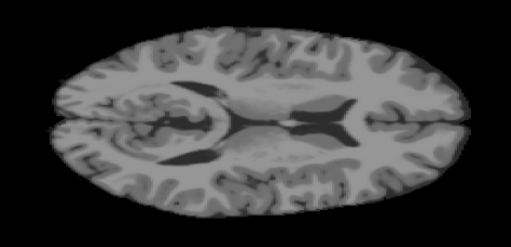
(b)
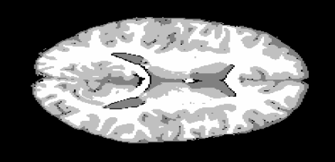
(b)

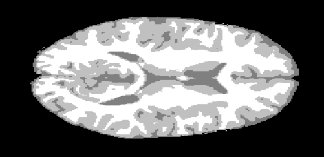
Fig. 1: (a) image to segment fom BrainWeb database, (b) ground truth image, (c) segmented image with HMRF-CS_Improved.

(a)
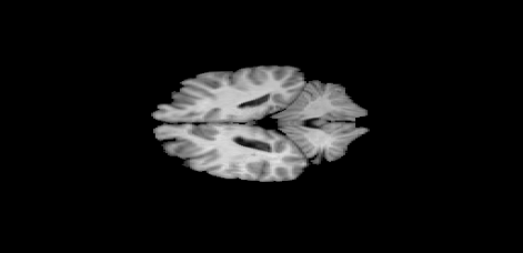
(b)
(b)

Fig. 2: (a) image to segment from IBSR database, (b) ground truth image, (c) segmented image using HMRF-CS_Improved.

5 CONCLUSIONS

In this paper, we have presented a new approach, that combines Hidden Markov Random Fields and cuckoo search to perform segmentation on MRI images. The tests conducted have focused on the brain images from largely used databases: BrainWeb and IBSR. The HMRF-CS_Improved combination outperforms other combination methods tested that are: HMRF-CS_Standard and CS_Auto. CS is simple, fast, robust and accurate. However, the proposed method needs to be tested on other images. A comparative study with other state-of-the-art segmentation methods also has to be conducted. A statistical study of parameters: $n,T,\mbox{step},\alpha,p_{a}$ is needed.

References

- [1] Stuart Geman and Donald Geman, “Stochastic relaxation, Gibbs distributions, and the bayesian restoration of images,” Pattern Analysis and Machine Intelligence, IEEE Transactions on, , no. 6, pp. 721–741, 1984.
- [2] Huawu Deng and David A Clausi, “Unsupervised image segmentation using a simple MRF model with a new implementation scheme,” Pattern recognition, vol. 37, no. 12, pp. 2323–2335, 2004.
- [3] Yongyue Zhang, Michael Brady, and Stephen Smith, “Segmentation of brain MR images through a hidden Markov random field model and the expectation-maximization algorithm,” IEEE transactions on medical imaging, vol. 20, no. 1, pp. 45–57, 2001.
- [4] Xin-She Yang and Suash Deb, “Cuckoo search via Lévy flights,” in 2009 World congress on nature & biologically inspired computing (NaBIC). IEEE, 2009, pp. 210–214.
- [5] Xin-She Yang and Suash Deb, “Engineering optimisation by cuckoo search,” arXiv preprint arXiv:1005.2908, 2010.
- [6] Xin-She Yang, Nature-inspired metaheuristic algorithms, Luniver press, 2010.
- [7] Ehsan Valian, Shahram Mohanna, and Saeed Tavakoli, “Improved cuckoo search algorithm for global optimization,” International Journal of Communications and Information Technology, vol. 1, no. 1, pp. 31–44, 2011.
- [8] Xiangtao Li and Minghao Yin, “Modified cuckoo search algorithm with self adaptive parameter method,” Information Sciences, vol. 298, pp. 80–97, 2015.
- [9] Lee R Dice, “Measures of the amount of ecologic association between species,” Ecology, vol. 26, no. 3, pp. 297–302, 1945.
- [10] EL-Hachemi Guerrout, Samy Ait-Aoudia, Dominique Michelucci, and Ramdane Mahiou, “Conjugate gradient method for brain magnetic resonance images segmentation,” in IFIP International Conference on Computational Intelligence and Its Applications. Springer, 2018, pp. 561–572.
- [11] Stephen Boyd and Lieven Vandenberghe, Convex optimization, Cambridge university press, 2004.
- [12] Xin-She Yang and Suash Deb, “Cuckoo search: recent advances and applications,” Neural Computing and Applications, vol. 24, no. 1, pp. 169–174, 2014.
- [13] Chris A Cocosco, Vasken Kollokian, Remi K-S Kwan, G Bruce Pike, and Alan C Evans, “Brainweb: Online interface to a 3D MRI simulated brain database,” 1997.