A Positive Resampler for Monte Carlo Events with Negative Weights

Abstract

We propose the Positive Resampler to solve the problem associated with event samples from state-of-the-art predictions for scattering processes at hadron colliders typically involving a sizeable number of events contributing with negative weight. The proposed method guarantees positive weights for all physical distributions, and a correct description of all observables. A desirable side product of the method is the possibility to reduce the size of event samples produced by General Purpose Event Generators, thus lowering the resource demands for subsequent computing-intensive event processing steps. We demonstrate the viability and efficiency of our approach by considering its application to a next-to-leading order + parton shower merged prediction for the production of a $W$ boson in association with multiple jets.

1 Introduction

General Purpose Event Generators Bellm:2015jjp ; Sjostrand:2014zea ; Bothmann:2019yzt form a crucial component of studies in high-energy physics, since they produce detailed predictions used for the design and calibration of detectors, interpretations of the measurements as well as the investigations of theoretical models. More often than not it is necessary to take into account the effects from the perturbative showering and the hadronisation models implemented in these generators, in order to achieve an accurate prediction for the cuts and observables chosen for experimental measurements.

High-accuracy perturbative event generator predictions can be obtained by first matching each jet multiplicity to next-to-leading order (NLO) using the methods of e.g. MC@NLO Frixione:2002ik or POWHEG Nason:2006hfa , followed by a merging of these exclusive samples using approaches such as MEPS@NLO Hoeche:2012yf or UNLOPS Lonnblad:2012ix ; Lonnblad:2012ng . The increased accuracy comes at a significant cost in additional computing resources, and these calculations increasingly contribute to the LHC computing footprint. The result of these merged NLO-accurate event generator simulations are event samples containing events of both positive and negative weights, meaning that the correspondence between the number of events in a bin of a distribution and the cross section in that bin is lost. Even when the event samples are unweighted to constitute events with weights of $\pm$1, the number of negative weighted events can be significant. This reduces the statistical significance of the sample compared to one with the same number of all positive weight events.

The outcome of event generation is often processed through time-consuming detector simulation – which currently constitutes the major part of the LHC computing budget. Since both positive and negative weight events are afterwards processed at a significant cost, it is beneficial to reduce the cancellation of events of negative and positive weight. This can be done by reducing the occurrence of negative weight events in the event generation, see e.g. Frederix:2020trv for an approach in MC@NLO.

We report here on an alternative and NLO-matching-independent approach to completely remove all negative weights from any already generated sample, and re-introducing the correspondence between the number of events in a bin and the local contribution to the cross section. This positive resampling will be achieved in a two-stage process: 1) modify the weights of events to be all positive and possibly smaller in magnitude, and 2) apply a standard unweighting. The second step should be taken only if the number of events is sought to be reduced. Reducing the event sample can significantly lower the computing budget for the steps in the analysis following the event generation, both in terms of CPU and disk. It may seem counter intuitive to allow for or even seek a reduction in the number of events, since traditionally the statistical significance of a sample, or the variance, is linked to the number of events, and reducing the number of events would therefore reduce the statistical significance of the sample. However, when the sample contains events with both positive and negative weights, the number of events can indeed be reduced without impacting the statistical significance: The effective cross section is given by $\sigma=\sigma_{p}-\sigma_{n}$, where $\sigma_{p}$ is the contribution from events with positive weights, and $\sigma_{n}$ that from negative weights. The Monte Carlo variance associated with the sample is $s_{p}^{2}/N_{p}+s_{n}^{2}/N_{n}$, where $s_{p}^{2},s_{n}^{2}$ is the variance of the integrand. If we replace the sample with one that has $N_{s}$ positively weighted events, the variance of this new sample is $s_{s}^{2}/N_{s}$. If therefore $N_{s}/(N_{p}+N_{n})$ is similar to $s_{s}/s_{p}$ or $s_{s}/s_{n}$, the variance can be unchanged. This is achieved with the Positive Resampler, a simplified description of which transforms the weight of each event to its absolute value and multiplies by $(\sigma_{p}-\sigma_{n})/(\sigma_{p}+\sigma_{n})$. If there is a large cancellation, then the weight of each event is much reduced, leading also to a reduction in the Monte Carlo estimate of the variance. Hence fewer events are needed for the same statistical certainty. The Positive Resampler is introduced in section 3, and section 4 showcases results obtained based on samples of $W\!+\!0,1,2$ jets at NLO fixed-order accuracy merged with UNLOPS.

2 Weights in UNLOPS merging

High-precision predictions are important ingredients to LHC data analysis. If the analysis is sensitive to the effect of yet higher jet multiplicities, high precision is obtained by “merging” several distinct calculations. NLO merged calculations provide the state-of-the-art for LHC phenomenology, and contribute significantly to the overall computing resource usage. At the same time, increased precision almost always comes at the cost of having to rely more heavily on weighted event generation. Typically, issues due to a reduction in statistical convergence worsen with every additional NLO calculation included in the merging.

NLO merging schemes aim to produce inclusive event samples that both comply with NLO fixed-order accuracy for several multi-jet processes, and ensure that the accuracy of parton showering is preserved. Various methods have been developed to this effect Hoeche:2012yf ; Lonnblad:2012ix ; Platzer:2012bs ; Hamilton:2012rf ; Alioli:2012fc ; Frederix:2012ps ; Bellm:2017ktr , all differing slightly in the concrete goals and the definition of the target accuracy. Each NLO merging method suffers from various sources of negative weights. Predictions based on unitarised merging schemes Lonnblad:2012ix are the only predictions that not only comply with both of the above criteria, but also guarantee that, for an arbitrary base process and arbitrary parton multiplicity, inclusive $n$-jet cross sections are preserved exactly, without introducing sub-dominant contributions due to the merging. This desirable feature comes at the price of introducing new sources of counter-events and/or event weights compared to other methods such as Hoeche:2012yf .

Hence, unitarised NLO merging provides a very non-trivial test of unweighting methods. In the following, we will employ the NLO merging as implemented in the Dire plugin to the Pythia event generator as a test case. This NLO merging implementation is based on UNLOPS Lonnblad:2012ix , includes QCD, QED and electroweak vector boson emissions, and thus allows merging of calculations with multiple hard jets, photons/leptons or electroweak vector bosons. In particular, the “EW-improved” merging of Christiansen:2015jpa is extended to NLO QCD. Unordered configurations (i.e. for which no history of ordered emissions can be reconstructed for an input event) are treated according to the MOPS+unordered prescription of Fischer:2017yja . The latter means that the merging also heavily relies on matrix elements extracted from MadGraph5_aMC@NLO Alwall:2014hca . Within this NLO merging framework, several sources of event weights arise:

• The input NLO QCD short-distance cross sections (generated with MadGraph5_aMC@NLO for this study) can contain positive and negative weights. The input events are typically unweighted to $\pm w$, where $w$ is a unit weight.

• The procedure of assigning a parton shower history to a high-multiplicity input event can necessitate weights. The history is chosen among all possible shower histories according to the shower probability, which may contain non-positive definite splitting functions in Dire. This leads to a corrective (positive or negative) weight.

• The merging procedure enforces a consistent renormalisation and factorisation scale setting by introducing weights. These weights are almost entirely positive and tend to fluctuate only mildly. The merging scheme further removes overlap between different input samples by including no-emission probabilities. These factors are essentially in $[0,1]$, but can, in rare cases (e.g. due to negative NLO parton distribution functions or splitting functions), lead to negative weights.

• The $\mathcal{O}(\alpha_{s})$ expansion of the weight discussed in the previous point – which is necessary to guarantee the NLO accuracy of the method – is often negative, thus introducing a non-negligible source of weights.

• The accuracy of inclusive cross sections is enforced by explicit unitarisation Lonnblad:2012ng ; Lonnblad:2012ix . This means that a large fraction of events will be employed as “counter-events” with negative weight.

• Independently of NLO merging, the subsequent showering may also generate event positive or negative weights if the splitting functions are not positive-definite.

The regions of phase space where negatively weighted events contribute most depends on the source of weights, and thus also on the merging setup. An overall larger fraction of negative weights can be expected when merging more NLO calculations. This is best illustrated with an example. Consider a precise background prediction for a vector-boson $+$ jets measurement. If only the inclusive zero-jet prediction is NLO accurate, then the predominant source of negative weights is the unitarisation of reweighted one-jet LO configurations. This will lead to a moderate amount of negatively weighted events, which produce a relatively flat negative contribution to the vector boson rapidity spectrum. The same events will induce larger negative weight fraction at small boson $p_{\perp V}$ than at high $p_{\perp V}$, since showering from counter-events is constrained to the soft/collinear regions. Negative weights will have a negligible impact on observables that require one, two or more jets. If the calculation is extended by also including an NLO calculation for the inclusive $V+$one-jet rate, then $p_{\perp V}$ will also exhibit negative-weight contributions at high values, since new sources of negative weights ($\mathcal{O}(\alpha_{s})$ expansions, unitarisation of the two-jet LO sample) arise. Observables that depend on two jets will now acquire a negative component at small jet separation due to the mechanism of unitarisation. This effect is illustrated in Figure 1.

3 A Positive Resampler

Our main goal is to restore the connection seen when generating all positive weight events between the number of events in the neighbourhood of any phase space point (e.g. the bin in any histogram) and the local contribution to the cross section. This will require a modification of the weight of all events in the neighbourhood of events with negative weights. The idea is simply stated to 1) calculate the cross section $\sigma_{i}$ from the $N_{i}$ positive and negative weight events in a neighbourhood, 2) change each weight to be positive and rescale all weights to preserve $\sigma_{i}$. One can then proceed with a unweighting procedure over all the neighbourhoods $i$ to restore the connection between the number of events and the cross section from each neighbourhood.

In Monte Carlo event generation, the cross sections are generated exclusively in all momenta. We will demonstrate first the method for the idealised situation where the cross section is stored differentially in all momenta relevant for the later event analysis – this could be e.g. momenta of the jets, leptons etc. We will then demonstrate how it works also in the case of using simple binned observables for the unweighting.

3.1 Multi-Dimensional Resampling

We begin by considering the idealistic case (i.e. the limit of infinitely narrow bin widths) where a differential distribution in the observable $\mathcal{O}_{1}$ is calculated with both positive and negative weight events in a $f$-body phase space region $\Omega_{f}$. The differential distribution in the observable $\mathcal{O}_{1}$ is then constructed as

$$\frac{\mathrm{d}\sigma}{\mathrm{d}\mathcal{O}_{1}}=\frac{\mathrm{d}\sigma}{\mathrm{d}\Omega_{f}}\ \frac{\mathrm{d}\Omega_{f}}{\mathrm{d}\Omega_{n}}\ \frac{\mathrm{d}\Omega_{n}}{\mathrm{d}\mathcal{O}_{1}},$$ (1)

where

• signifies the cross section calculated in terms of the final state momenta.

• encodes e.g. the jet clustering and is the Jacobian for the $f$-body phase space into the $n$-body phase space ($n<f$) that the observable depends on.

• is traditionally included in the calculations by the binning of the $n$-body phase space in terms of $\mathcal{O}_{1}$.

Equation (1) just constitutes the chain rule of differentiation. Histogrammed distributions are obtained by simple integrations of this relation. It is therefore not surprising that if the events of positive and negative weights arising in the generation (represented by $\frac{\mathrm{d}\sigma}{\mathrm{d}\Omega_{f}}$) can be turned into events of all positive weights, then the distribution in any $\mathcal{O}_{1}$ can be calculated with these events (since the calculation of the other factors in equation (1) are unchanged). Of course the $f$-body phase space can have a very high dimension and it may seem impractical to perform the clustering of events in bins in all the dimensions of $\Omega_{f}$ followed by the reweighting procedure outlined above. One could of course perform the reweighting in the lower-dimensional $\Omega_{n}$, the phase space of all objects (jets etc.) entering observables. It is clear here that the reweighting works for any observable $\Omega_{1}$. What is perhaps surprising is that if the reweighting is performed in neighbourhoods (bins after integration) in $\mathcal{O}_{1}$ then $\frac{\mathrm{d}\sigma}{\mathrm{d}\mathcal{O}_{2}}$ for any other observable $\mathcal{O}_{2}$ can still be constructed: We have

$$\frac{\mathrm{d}\sigma}{\mathrm{d}\mathcal{O}_{2}}=\frac{\mathrm{d}\Omega_{f}}{\mathrm{d}\mathcal{O}_{2}}\ \left\{\left(\frac{\mathrm{d}\sigma}{\mathrm{d}\Omega_{f}}\ \frac{\mathrm{d}\Omega_{f}}{\mathrm{d}\Omega_{n}}\ \frac{\mathrm{d}\Omega_{n}}{\mathrm{d}\mathcal{O}_{1}}\ \right)\ \frac{\mathrm{d}\mathcal{O}_{1}}{\mathrm{d}\Omega_{f}}\right\}.$$ (2)

All reference to the cross section $\sigma$ is within the brackets $(\cdots)$, so the cancellation of positive and negative weight events can be implemented here in terms of reweighting as above to the distribution in $\mathcal{O}_{1}$. The effect of $\mathrm{d}\mathcal{O}_{1}/\mathrm{d}\Omega_{f}$ is taken into account by calculating the value (or bin) of $\mathcal{O}_{1}$ starting from the phase space points in $\Omega_{f}$. The spectrum for the observable $\mathcal{O}_{2}$ is then calculated by constructing the quantities

• by binning the contribution from the phase space points in $\mathcal{O}_{f}$ in terms of the observable $\mathcal{O}_{2}$

• by finding all $\Omega_{f}$ resulting in $\mathcal{O}_{1}$, and multiply by the differential distribution in $\mathcal{O}_{1}$.

So, in terms of truly differential distributions, it would not matter which observable $\mathcal{O}_{i}$ one would start from. The distribution in $\mathcal{O}_{j}$ can be obtained by the procedure above. This is correct up to effects in the binning in $\mathcal{O}_{1}$, which we will later show are modest indeed, and can be reduced further by decreasing the bin widths used in the Positive Resampler. Indeed, in the situation where the impact of the negative weight events in phase space $\Omega_{f}$ mapped into the equivalent bins in $\mathcal{O}_{1}$ and $\mathcal{O}_{2}$ is identical, then the result for $\mathcal{O}_{2}$ using the Positive Resampler in $\mathcal{O}_{1}$ is exact. We will see in section 4.1 how convergence can be achieved by sampling in multiple dimensions.

3.2 Resampling the total cross section

The extreme opposite of resampling in all $n$ dimensions of the momenta of constructs used in the analysis, such as jets and leptons, is resampling just the cross section – effectively using just one bin. As we will see in section 4 even this extreme yields reasonable results using the method described in this section. It may be considered coarse, but we include the discussion here since it provides a simple example of the algorithms used. For clarity, we choose to illustrate the method in terms of bins and weights, obtained as integrals and MC sampling of the distributions discussed in section 3.1.

Let us start by considering the total cross section

$$\sigma=\sum_{i=1}^{N}w_{i}\,,$$ (3)

obtained from $N$ events with weights $w_{i}$. Introducing a convenient factor of one, we can write

$$\sigma=\sum_{i=1}^{N}w_{i}=\frac{\left(\sum_{i=1}^{N}|w_{i}|\right)\left(\sum_{i=1}^{N}w_{i}\right)}{\sum_{i=1}^{N}|w_{i}|}\equiv P\sum_{i=1}^{N}|w_{i}|\,,$$ (4)

where $0\leq P=\tfrac{\sum_{i}w_{i}}{\sum_{i}|w_{i}|}\leq 1$. Effectively, this amounts to replacing each event weight $w_{i}$ by $P|w_{i}|$. The total cross section is preserved by construction, but what is the effect on binned distributions?

To answer this question, let us select an arbitrary distribution $\tfrac{d\sigma}{d\mathcal{O}}$ and an arbitrary bin $B$ ranging from $\mathcal{O}_{B}$ to $\mathcal{O}_{B+1}$ and containing $M\gg 1$ events. Without loss of generality we can assume that the bin contains the events $i=1,\dots,M$. The height of the bin is given by

$$\sigma_{\mathcal{O},B}\equiv\frac{d\sigma}{d\mathcal{O}}(\mathcal{O}_{B+1}-\mathcal{O}_{B})=\sum_{i=1}^{M}w_{i}=\frac{\sum_{i=1}^{N}|w_{i}|}{\sum_{i=1}^{N}|w_{i}|}\sum_{i=1}^{M}w_{i}\,,$$ (5)

where we have introduced the same factor of one as previously. In the simplified case with a uniform distribution of negative weights,

$$\frac{\sum_{i=1}^{M}w_{i}}{\sum_{i=1}^{M}|w_{i}|}\approx\frac{\sum_{i=1}^{N}w_{i}}{\sum_{i=1}^{N}|w_{i}|}\,,$$ (6)

we can effectively swap the summation limits in the numerator of the equation (5) for the bin height:

$$\sigma_{\mathcal{O},B}=\sum_{i=1}^{M}w_{i}=\frac{\sum_{i=1}^{N}|w_{i}|}{\sum_{i=1}^{N}|w_{i}|}\sum_{i=1}^{M}w_{i}\approx\frac{\sum_{i=1}^{N}w_{i}}{\sum_{i=1}^{N}|w_{i}|}\sum_{i=1}^{M}|w_{i}|=P\sum_{i=1}^{M}|w_{i}|\,.$$ (7)

This tells us that simply replacing each event weight $w_{i}$ by $P|w_{i}|$ preserves the total cross section exactly and also all bin heights in each distribution in the limit of large statistics, i.e. within statistical fluctuations for finite statistics. In practice, negative weights will not necessarily be distributed uniformly. We will analyse the real-world performance for the example of W + jets production in section 4.

3.3 Resampling a distribution

For one-dimensional sampling in terms of an observable $\mathcal{O}$, the method can be adapted to preserve exactly the distribution in $\mathcal{O}$. The accuracy in other distribution will be determined by the variation in the impact of negative weight events for the phase space $\Omega_{f}$ mapped into each bin in the two distributions. In analogy to equation (4) we introduce separate rescaling factors $P_{\mathcal{O},B}$ for each bin $B$ containing the events $i=i_{B},\dots,i_{B+1}$:

$$\sigma_{\mathcal{O},B}=\sum_{i=i_{B}}^{i_{B+1}}w_{i}=\frac{\sum_{i=i_{B}}^{i_{B+1}}|w_{i}|}{\sum_{i=i_{B}}^{i_{B+1}}|w_{i}|}\sum_{i=i_{B}}^{i_{B+1}}w_{i}\equiv P_{\mathcal{O},B}\sum_{i=i_{B}}^{i_{B+1}}|w_{i}|\,.$$ (8)

This preserves all bin heights exactly and therefore the full distribution in $\mathcal{O}$. The total cross section is just the sum over all bins, which also remains unchanged. In cases where the systematic variation in the distribution of negative weights is negligible, eq. (6) guarantees that all rescaling factors $P_{\mathcal{O^{\prime}},B^{\prime}}$ for all observables $\mathcal{O^{\prime}}$ and bins $B^{\prime}$ converge to the same value. This implies that all other distributions remain correct in the limit of large statistics.

It is straightforward to generalise the argument to multi-differential distributions. For instance, if we resample bins in a double-differential distribution in $\mathcal{O}$ and $\mathcal{O}^{\prime}$ then also the respective single-differential distributions in $\mathcal{O}$ and $\mathcal{O}^{\prime}$ as well as the total cross section are preserved exactly. The most extreme case is a differential distribution in all final-state momenta. In the limit of infinitesimal bin widths we recover the idealised scenario already described in section 3.1. The convergence to the correct result can be achieved by appropriately increasing the dimensions used in the Positive Resampler.

4 Results from the Positive Resampler

To demonstrate the practical performance of the algorithm outlined in section 3 we consider an $\alpha_{s}$-driven NLO-merged description of the $W$-boson $+$ jets process, as an example of a resource-intense calculation. We focus on results for proton-proton collisions at 14 TeV centre-of-mass energy. The inclusive event sample merging NLO QCD calculations for 0, 1 and 2 additional jets is generated by using MadGraph5_aMC@NLO merged and showered by Dire. Multiparton interactions, hadronisation and beam remnants are handled by Pythia. The outputs are analysed using Rivet Bierlich:2019rhm , which provides the input distributions to the Positive Resampler, and performs the analysis and plotting. We present results for the standard Rivet analyses MC_WINC and MC_WJETS in order to illustrate the performance of the Positive Resampler on analyses already in use by the community for testing the description of the production of a $W$-boson.

We then apply a series of resampling steps to the generated weighted event samples. We first choose a target (binned) distribution which we aim to preserve exactly during the procedure. We are free to pick an arbitrary distribution for this purpose. In the present work, we consider first the following one-dimensional examples.

• W boson transverse momentum. We preserve $\tfrac{d\sigma}{dp_{W\perp}}$, in bins with a width of 5 GeV each. In the peak region $p_{W\perp}<125\,$GeV this coincides with a histogram from the MC_WINC Rivet analysis.

• Parton shower evolution variable $t$. This unmeasurable parameter is defined as the Dire parton shower ordering variable Hoche:2015sya at which a zero-parton state transitions to a one-parton state. For events with more than zero partons before showering, we use the $t$-value of the first node in the reconstructed parton-shower history that is employed when calculating no-emission probabilities within UNLOPS. If no transition from a zero- to a one-parton state exists (e.g. if the shower did not perform an emission, or if the history favoured electroweak clusterings), we set $t=-1$. For $t>0$, we consider $\tfrac{d\sigma}{d\log t}$ in $\sqrt{N}$ bins, where $N$ is the number of events in each sample. We add one more bin for events with $t<0$.

• Total cross section. All events are contained in a single bin.

Our aim here is to demonstrate the viability of positive resampling independently of the concrete analysis. For this reason we generally consider distributions for the complete event samples and refrain from applying any analysis cuts at this stage. The exception is option a), where the Rivet analysis is used for identifying the momentum of the W boson.

In the next step, we apply the following procedure to each bin in the chosen distribution. These are the same steps later applied in each bin of multi-dimensional sampling.

1. Change weights. We turn negative-weight into positive-weight events as described in section 3. This preserves the height of each bin exactly.

2. Partial unweighting. We choose a target weight $W_{t}$ and apply standard unweighting to all events with weights $w_{t}<W_{t}$, i.e. we keep the event with probability $p=\tfrac{w_{t}}{W_{t}}$ and then adjust the event weight to $W_{t}$. We choose $W_{t}$ in such a way that approximately $10\%$ of the original events are kept. This number can straightforwardly be adjusted.

3. Bin restoration. We rescale the weights of all events in the bin such that the original bin height is restored. If the stochastic unweighting in the previous step resulted in an empty bin, we first pick a random discarded event and add it back to the bin prior to restoring the height. The probability to recover a discarded event is chosen to be proportional to its weight.

We also compare our approach to more traditional unweighting, where the signs of the event weights are unchanged, and the modulus of the event weight is used when deciding whether an event should be kept.

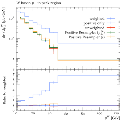
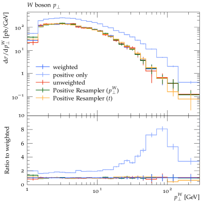
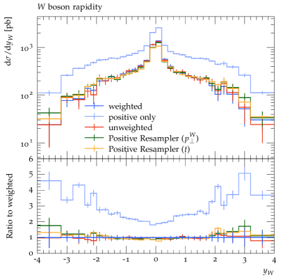
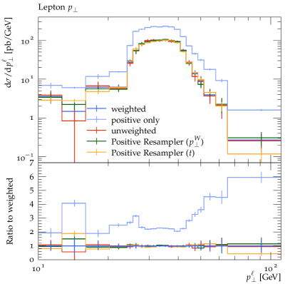
Figure 1: The distributions of $p_{\perp}^{W}$, $y_{W}$ and $p^{l}_{\perp}$ obtained using the various samples. The sample of “positive only” events is included to illustrate the scale of the contribution from negative weight events.

As is illustrated on Figure 1, the results obtained using both traditional unweighting and the Positive Resampler are consistent with the result using all events, well within the statistical fluctuation of that largest sample. It is also clear that the statistical uncertainty associated with the distributions obtained with the Positive Resampler is similar to that of the input weighted distribution. The central values and associated uncertainty is for both calculated by Rivet.

To some degree, the power of the method is in the reduction of events necessary to achieve a certain statistical accuracy.

Sample	Total number of events	Events included in analysis
weighted	5.3M	195k
positive only	3.2M	121k
unweighted	1.5M	52k
Positive Resampler($t$)	659k	25k
Positive Resampler($p_{\perp}^{W}$)	33k	33k

Table 1: The number of events generated in the sample of $W+0j,1j,2j$@NLO merged with UNLOPS (weighted), and the number of events arising from these by using the algorithms discussed in the paper.

Table 1 lists the number of events in each sample; the input test sample to the Positive Resampler contains 5.3M events, of which 195k pass the cuts of the analysis. Of these, 3.2M and 121k respectively have positive weights. The simple unweighting procedure leaves 1.5M (52k passing cuts of the analysis). The Positive Resampler according to $t$ reduces this to 659k and 25k respectively. The Positive Resampler($p_{\perp}^{W}$) by construction accepts events only if they pass the cuts of the analysis, which with this resampling is 33k. The true power of the positive resampling is in the reduction from 52k to 25k or 33k of events. This reduction in the number of events is brought about by the cancellation between positive and negative contributions, illustrated in Figure 1 by the contribution of “positive only”. The fact that this contribution is roughly twice the cross section at the peak of the distribution (most easily checked for $y_{w}$) leads directly to the reduction in the number of events obtained with the Positive Resampler. The increasing ratio of the “positive only” to the “weighted” result at large $p^{W}_{\perp}$ and $p_{\perp}^{l}$ is a result of the increasing cancellations taking place within the input sample as discussed in section 2. It is these cancellations that the Positive Resampler implements effectively by reducing the event count. The number of events left after the resampling can be adjusted and tuned – the largest possible number of events per unit of cross section is given by the number of events (positive and negative) in the bin with the least cancellation, divided by the cross section in this bin. The distributions expose large cancellations in some regions of phase space, indicating that many more events are required to obtain statistically meaningful spectra. Improvements of the example NLO-merging implementation used – to reduce the amount of cancellation already at the “weighted” stage – would clearly be beneficial Frederix:2020trv .

4.1 Positive Resampling in Higher Dimensions

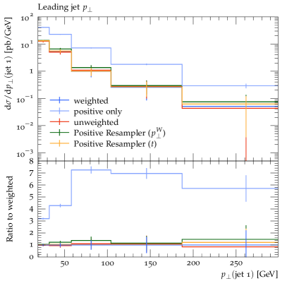
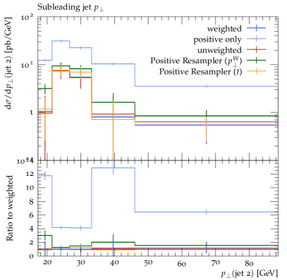
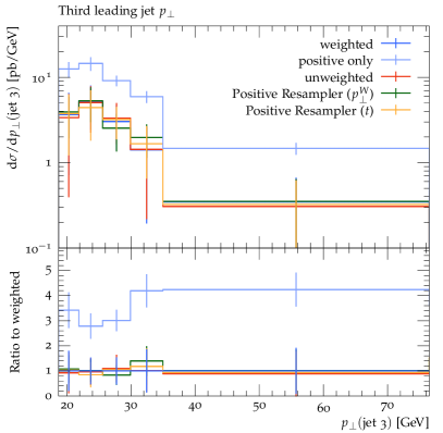
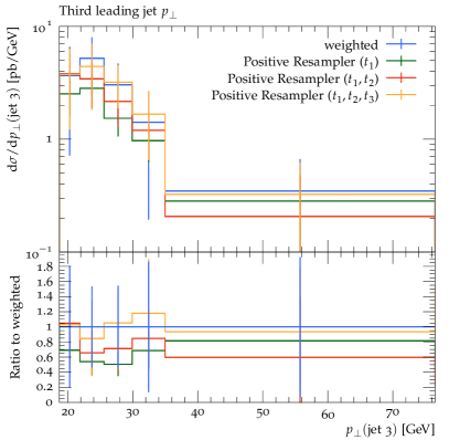
Figure 2: The transverse momentum of the hardest jet ($p^{j_{1}}_{\perp}$), second hardest jet ($p^{j_{2}}_{\perp}$), and third hardest jet ($p^{j_{3}}_{\perp}$). The lower right plot shows the convergence of the result of the Positive Resampler for an increasing number of dimensions using the shower evolution variable of up to three emissions.

The distributions studied in the previous section all relate to the momenta of the $W$ and its decay products. Figure 2 presents results for the transverse momentum distribution of the three hardest jets produced in association with the $W$. Following the discussion in section 3.1 on multi-dimensional resampling for processes with many final state momenta of leptons and jets , it is unsurprising that a good description of the transverse momentum of the third jet requires sampling in more than just one dimension. Perhaps the surprising result is how few extra dimensions are required for a good description. The lower right pane on Figure 2 shows the description of $p_{\perp}^{j_{3}}$ when the Positive Resampler is applied in an increasing number of dimensions from 1 to 3, using the shower evolution variable for the first, second and third hardest emission. The result converges to the weighted result (the input to the resampler) as the number of dimensions used in the resampling is increased, and using three dimensions it is already well within the statistical fluctuations of the sample (some statistical fluctuation is obviously expected from the stochastical process of unweighting).

The result for the transverse momentum spectrum for the leading, subleading and the third leading jet is presented on the three remaining plots of Figure 2. The result for the Positive Resampler in $p_{\perp}^{W}$ uses just one-dimensional resampling, whereas that of Positive Resampler($t$) uses the three-dimensional resampling in the shower evolution variable. The curve for positive only illustrates again the significance of the negative weight events in the sample, and the portion of the events that can be removed. Resampling in three scalar dimensions is sufficient for the description of all the momenta.

5 Conclusions

We presented the Positive Resampler, a method for modifying the weights of events drawn from a sample with both positive and negative weights, such that all events enter with positive weights, while kinematic distributions and observables are preserved exactly or within the statistical variations in the sample. The method was demonstrated using reweighting in three different distributions and the impact on 6 independent observables studied. Since weight cancellations are handled explicitly, the reweighting can be implemented through a reduction of the number of events, thus allowing to significantly lower the cost and time associated with post-processing the event sample with subsequent analysis and modelling. The implementation of the reweighter used in this study will be publicly available after publication of this manuscript.

References

- (1) J. Bellm et al., Herwig 7.0/Herwig++ 3.0 release note, Eur. Phys. J. C76 (2016) 196, [1512.01178].
- (2) T. Sjöstrand, S. Ask, J. R. Christiansen, R. Corke, N. Desai, P. Ilten et al., An Introduction to PYTHIA 8.2, Comput. Phys. Commun. 191 (2015) 159–177, [1410.3012].
- (3) Sherpa collaboration, E. Bothmann et al., Event Generation with Sherpa 2.2, SciPost Phys. 7 (2019) 034, [1905.09127].
- (4) S. Frixione and B. R. Webber, Matching NLO QCD computations and parton shower simulations, JHEP 06 (2002) 029, [hep-ph/0204244].
- (5) P. Nason and G. Ridolfi, A Positive-weight next-to-leading-order Monte Carlo for Z pair hadroproduction, JHEP 08 (2006) 077, [hep-ph/0606275].
- (6) S. Höche, F. Krauss, M. Schönherr and F. Siegert, QCD matrix elements + parton showers: The NLO case, JHEP 04 (2013) 027, [1207.5030].
- (7) L. Lönnblad and S. Prestel, Merging Multi-leg NLO Matrix Elements with Parton Showers, JHEP 03 (2013) 166, [1211.7278].
- (8) L. Lönnblad and S. Prestel, Unitarising Matrix Element + Parton Shower merging, JHEP 02 (2013) 094, [1211.4827].
- (9) R. Frederix, S. Frixione, S. Prestel and P. Torrielli, On the reduction of negative weights in MC@NLO-type matching procedures, 2002.12716.
- (10) S. Plätzer, Controlling inclusive cross sections in parton shower + matrix element merging, JHEP 08 (2013) 114, [1211.5467].
- (11) K. Hamilton, P. Nason, C. Oleari and G. Zanderighi, Merging H/W/Z + 0 and 1 jet at NLO with no merging scale: a path to parton shower + NNLO matching, JHEP 05 (2013) 082, [1212.4504].
- (12) S. Alioli, C. W. Bauer, C. J. Berggren, A. Hornig, F. J. Tackmann, C. K. Vermilion et al., Combining Higher-Order Resummation with Multiple NLO Calculations and Parton Showers in GENEVA, JHEP 09 (2013) 120, [1211.7049].
- (13) R. Frederix and S. Frixione, Merging meets matching in MC@NLO, JHEP 12 (2012) 061, [1209.6215].
- (14) J. Bellm, S. Gieseke and S. Plätzer, Merging NLO Multi-jet Calculations with Improved Unitarization, Eur. Phys. J. C 78 (2018) 244, [1705.06700].
- (15) S. Alioli, A. Broggio, S. Kallweit, M. A. Lim and L. Rottoli, Higgsstrahlung at NNLL’NNLO matched to parton showers in GENEVA, Phys. Rev. D 100 (2019) 096016, [1909.02026].
- (16) R. Frederix and K. Hamilton, Extending the MINLO method, JHEP 05 (2016) 042, [1512.02663].
- (17) J. R. Christiansen and S. Prestel, Merging weak and QCD showers with matrix elements, Eur. Phys. J. C 76 (2016) 39, [1510.01517].
- (18) N. Fischer and S. Prestel, Combining states without scale hierarchies with ordered parton showers, Eur. Phys. J. C 77 (2017) 601, [1706.06218].
- (19) J. Alwall, R. Frederix, S. Frixione, V. Hirschi, F. Maltoni, O. Mattelaer et al., The automated computation of tree-level and next-to-leading order differential cross sections, and their matching to parton shower simulations, JHEP 07 (2014) 079, [1405.0301].
- (20) C. Bierlich et al., Robust Independent Validation of Experiment and Theory: Rivet version 3, SciPost Phys. 8 (2020) 026, [1912.05451].
- (21) S. Höche and S. Prestel, The midpoint between dipole and parton showers, Eur. Phys. J. C 75 (2015) 461, [1506.05057].