Enhancing Certified Robustness via Smoothed Weighted Ensembling

Abstract

Randomized smoothing has achieved state-of-the-art certified robustness against $l_{2}$-norm adversarial attacks. However, it is not wholly resolved on how to find the optimal base classifier for randomized smoothing. In this work, we employ a Smoothed WEighted ENsembling (SWEEN) scheme to improve the performance of randomized smoothed classifiers. We show the ensembling generality that SWEEN can help achieve optimal certified robustness. Furthermore, theoretical analysis proves that the optimal SWEEN model can be obtained from training under mild assumptions. We also develop an adaptive prediction algorithm to reduce the prediction and certification cost of SWEEN models. Extensive experiments show that SWEEN models outperform the upper envelope of their corresponding candidate models by a large margin. Moreover, SWEEN models constructed using a few small models can achieve comparable performance to a single large model with a notable reduction in training time.

1 Introduction

Deep neural networks have achieved great success in image classification tasks. However, they are vulnerable to adversarial examples, which are small imperceptible perturbations on the original inputs that can cause misclassification [Biggio et al., 2013, Szegedy et al., 2014]. To tackle this problem, researchers have proposed various defense methods to train classifiers robust to adversarial perturbations. These defenses can be roughly categorized into empirical defenses and certified defenses. One of the most successful empirical defenses is adversarial training [Kurakin et al., 2017, Madry et al., 2018], which optimizes the model by minimizing the loss over adversarial examples generated during training. Empirical defenses produce models robust to certain attacks without a theoretical guarantee. Most of the empirical defenses are heuristic and subsequently broken by more sophisticated adversaries [Carlini and Wagner, 2017, Athalye et al., 2018, Uesato et al., 2018, Tramer et al., 2020]. Certified defenses, either exact or conservative, are introduced to mitigate such deficiency in empirical defenses. In the context of $l_{p}$ norm-bounded perturbations, exact methods report whether an adversarial example exists within an $l_{p}$ ball with radius $r$ centered at a given input $x$. Exact methods are usually based on Satisfiability Modulo Theories [Katz et al., 2017, Ehlers, 2017] or mixed-integer linear programming [Lomuscio and Maganti, 2017, Fischetti and Jo, 2017], which are computationally inefficient and not scalable [Tjeng et al., 2019]. Conservative methods are more computationally efficient, but might mistakenly flag a safe data point as vulnerable to adversarial examples [Raghunathan et al., 2018a, Wong and Kolter, 2018, Wong et al., 2018, Gehr et al., 2018, Mirman et al., 2018, Weng et al., 2018, Zhang et al., 2018, Raghunathan et al., 2018b, Dvijotham et al., 2018b, Singh et al., 2018, Wang et al., 2018b, Salman et al., 2019b, Croce et al., 2019, Gowal et al., 2018, Dvijotham et al., 2018a, Wang et al., 2018a]. However, both types of defenses are not scalable to practical networks that perform well on modern machine learning problems (e.g., the ImageNet [Deng et al., 2009] classification task).

Recently, a new certified defense technique called randomized smoothing has been proposed [Lecuyer et al., 2019, Cohen et al., 2019]. A (randomized) smoothed classifier is constructed from a base classifier, typically a deep neural network. It outputs the most probable class given by its base classifier under a random noise perturbation of the input. Randomized smoothing is scalable due to its independency over architectures and has achieved state-of-the-art certified $l_{2}$-robustness. In theory, randomized smoothing can apply to any classifiers. However, naively using randomized smoothing on standard-trained classifiers leads to poor robustness results. It is still not wholly resolved on how a base classifier should be trained so that the corresponding smoothed classifier has good robustness properties. Recently, Salman et al. [2019a] employ adversarial training to train base classifiers and substantially improve the performance of randomized smoothing, which indicates that techniques originally proposed for empirical defenses can be useful in finding good base classifiers for randomized smoothing.

In this paper, we take a step towards finding suitable base models for randomized smoothing by model ensembling. The idea of model ensembling has been used in various empirical defenses against adversarial examples and shows promising results for robustness [Liu et al., 2018, Strauss et al., 2018, Pang et al., 2019, Wang et al., 2019, Meng et al., 2020, Sen et al., 2020]. Moreover, an ensemble can combine the strengths of candidate models to achieve superior clean accuracy [Hansen and Salamon, 1990, Krogh and Vedelsby, 1994]. Thus, we believe ensembling several smoothed models can help improve both the robustness and accuracy. Specifically for randomized smoothing, the smoothing operator is commutative with the ensembling operator: ensembling several smoothed models is equivalent to smoothing an ensembled base model. This property makes the combination suitable and efficient. Therefore, we directly ensemble a base model by taking some pre-trained models as candidates and optimizing the optimal weights for randomized smoothing. We refer to the final model as a Smoothed WEighted ENsembling (SWEEN) model. Moreover, SWEEN does not limit how individual candidate classifiers are trained, thus is compatible with most previously proposed training algorithms on randomized smoothing.

Our contributions are summarized as follows:

1. We propose SWEEN to substantially improve the performance of smoothed models. Theoretical analysis shows the ensembling generality and the optimization guarantee: SWEEN can achieve optimal certified robustness w.r.t. the defined $\gamma$-robustness index, which is an extension of previously proposed criteria of certified robustness (Lemma 1), and SWEEN can be easily trained to a near-optimal risk with a surrogate loss (Theorem 2).

2. We develop an adaptive prediction algorithm for the weighted ensembling, which effectively reduces the prediction and certification cost of the smoothed ensemble classifier.

3. We evaluate our proposed method through extensive experiments. On all tasks, SWEEN models outperform the upper envelopes of their respective candidate models in terms of the approximated certified accuracy by a large margin. To the best of our knowledge, our best results achieve the state-of-the-art certified robustness on CIFAR-10 under $\ell_{2}$ norm. In addition, SWEEN models can achieve comparable or superior performance to a large individual model using a few candidates with a notable reduction in total training time.

2 Related Work

In the past few years, numerous defenses have been proposed to build classifiers robust to adversarial examples. Our work typically involves randomized smoothing and model ensembling.

Randomized smoothing  Randomized smoothing constructs a smoothed classifier from a base classifier via convolution between the input distribution and certain noise distribution. It is first proposed as a heuristic defense by [Liu et al., 2018, Cao and Gong, 2017]. Lecuyer et al. [2019] first prove robustness guarantees for randomized smoothing utilizing tools from differential privacy. Subsequently, a stronger robustness guarantee is given by Li et al. [2018]. Cohen et al. [2019] provide a tight robustness bound for isotropic Gaussian noise in $l_{2}$ robustness setting. The theoretical properties of randomized smoothing in various norm and noise distribution settings have been further discussed in the literature [Blum et al., 2020, Kumar et al., 2020, Yang et al., 2020, Lee et al., 2019, Teng et al., 2019, Zhang et al., 2020]. Recently, a series of works [Salman et al., 2019a, Zhai et al., 2020] develop practical algorithms to train a base classifier for randomized smoothing. Our work improves the performance of smoothed classifiers via weighted ensembling of pre-trained base classifiers.

Model ensembling  Model ensembling has been widely studied and applied in machine learning as a technique to improve the generalization performance of the model [Hansen and Salamon, 1990, Krogh and Vedelsby, 1994]. Krogh and Vedelsby [1994] show that ensembles constructed from accurate and diverse networks perform better. Recently, simple averaging of multiple neural networks has been a success in ILSVRC competitions [He et al., 2016, Krizhevsky et al., 2017, Simonyan and Zisserman, 2015]. Model ensembling has also been used in defenses against adversarial examples [Liu et al., 2018, Strauss et al., 2018, Pang et al., 2019, Wang et al., 2019, Meng et al., 2020, Sen et al., 2020]. Wang et al. [2019] have shown that a jointly trained ensemble of noise injected ResNets can improve clean and robust accuracies. Recently, Meng et al. [2020] find that ensembling diverse weak models can be quite robust to adversarial attacks. Unlike the above works, which are empirical or heuristic, we employ ensembling in randomized smoothing to provide a theoretical robustness certification.

3 Preliminaries

Notation  Let $\mathcal{Y}=\{1,2,...,M\}$. We overload notation slightly, letting $k$ refer the $M$-dimensional one-hot vector whose $k$-th entry is $1$ for $k=1,...,M$ as well. The choice should be clear from context. Let $\Delta_{k}=\{(p_{1},p_{2},...,p_{k})\big{|}p_{i}\geq 0,\sum_{i=1}^{k}p_{i}=1\}$ be the $k$-dimensional probability simplex for $k\in\mathbb{N}_{+}$, and $\Delta=\Delta_{M}$. For an $M$-dimensional function $f$, we use $f_{i}$ to refer to its $i$-th entry, $i=1,2,\cdots,M$. We use $\mathcal{N}(0,\sigma^{2}I)$ to denote the $d$-dimensional Gaussian distribution with mean 0 and variance $\sigma^{2}I$. We use $\Phi^{-1}$ to denote the inverse of the standard Gaussian CDF, and use $\Gamma$ to denote the gamma function. We use $\mathbb{R}^{*}$ to denote the set of non-negative real numbers. For $x,a,b\in\mathbb{R},a\leq b$, we define $\mathrm{clip}(x;a,b)=\min\{\max\{x,a\},b\}$. We use $\Omega(\cdot)$ to denote Big-Omega notation that suppresses multiplicative constants.

Neural network and classifier  Consider a classification problem from $\mathcal{X}\subseteq\mathbb{R}^{d}$ to classes $\mathcal{Y}$. Assume the input space $\mathcal{X}$ has finite diameter $D=\sup_{x_{1},x_{2}\in\mathcal{X}}\|x_{1}-x_{2}\|_{2}<\infty$. The training set $\{(x_{i},y_{i})\}_{i=1}^{n}$ is i.i.d. drawn from the data distribution $\mathcal{D}$. We call $f$ a probability function or a classifier if it is a mapping from $\mathbb{R}^{d}$ to $\Delta$ or $\mathcal{Y}$, respectively. For a probability function $f$, its induced classifier $f^{*}$ is defined such that $f^{*}(x)=\mathop{\arg\max}_{1\leq i\leq M}f_{i}(x)$. For simplicity, we will not distinguish between $f$ and $f^{*}$ when there is no ambiguity, and hence all definitions and properties for classifiers automatically apply to probability functions as well. $f(\cdot;\theta)$ denotes a neural network parameterized by $\theta\in\Theta$. Here $\Theta$ can include hyper-parameters, thus the architectures of $f(\cdot;\theta)$’s do not have to be identical.

Certified robustness  We call $x+\delta$ an adversarial example of a classifier $f$, if $f$ correctly classifies $x$ but $f(x+\delta)\neq f(x)$. Usually $\|\delta\|_{2}$ is small enough so $x+\delta$ and $x$ appear almost identical for the human eye. The ($l_{2}$-)robust radius of $f$ is defined as

$$r(x,y;f)=\inf_{F(x+\delta)\neq y}\|\delta\|_{2},$$ (1)

which is the radius of the largest $l_{2}$ ball centered at $x$ within which $f$ consistently predicts the true label $y$ of $x$. Note that $r(x,y;f)=0$ if $f(x)\neq y$. As mentioned before, we can extend the above definitions to the case when $f$ is a probability function by considering the induced classifier $f^{*}$. A certified robustness method tries to find some lower bound $r_{c}(x,y;f)$ of $r(x,y;f)$, and we call $r_{c}$ a certified radius of $f$.

Randomized smoothing  Let $f$ be a probability function or a classifier. The (randomized) smoothed function of $f$ is defined as

$$g(x)=\mathbb{E}_{\delta\sim\mathcal{N}(0,\sigma^{2}I)}[f(x+\delta)].$$ (2)

The (randomized) smoothed classifier of $f$ is then defined as $g^{*}$. Cohen et al. [2019] first provide a tight robustness guarantee for classifier-based smoothed classifiers, which is summerized in the following theorem:

Theorem 1.

(Cohen et al. [2019]) For any classifier $f$, denote its smoothed function by $g$. Then

$$r(x,y;g)\geq\frac{\sigma}{2}[\Phi^{-1}(g_{y}(x))-\Phi^{-1}(\max_{k\neq y}g_{k}(x))].$$ (3)

Later on, Salman et al. [2019a], Zhai et al. [2020] extends Theorem 1 for probability functions.

4 SWEEN: Smoothed weighted ensembling

In this section, we describe the SWEEN framework we use. We also present some theoretical results for SWEEN models. The proofs of the results in this section can be found in Appendix A.

4.1 SWEEN: Overview

To be specific, we adopt a data-dependent weighted average of neural networks to serve as the base model for smoothing. Suppose we have some pre-trained neural networks $f(\cdot;\theta_{1}),...,f(\cdot;\theta_{K})$ as ensemble candidates. A weighted ensemble model is then

$$f_{ens}(\cdot;\theta,w)=\sum_{k=1}^{K}w_{k}f(\cdot;\theta_{k}),$$ (4)

where $\theta=(\theta_{1},\cdots,\theta_{K})\in\Theta^{K}$, and $w\in\Delta_{K}$ is the ensemble weight. For a specific $f_{ens}$, the corresponding SWEEN model is defined as the smoothed function of $f_{ens}$, denoted by $g_{ens}$. We have

$$\begin{split}g_{ens}(x;\theta,w)&=\mathbb{E}_{\delta}[\sum_{k=1}^{K}w_{k}f(x+\delta;\theta_{k})]\\ &=\sum_{k=1}^{K}w_{k}\mathbb{E}_{\delta}f(x+\delta;\theta_{k})=\sum_{k=1}^{K}w_{k}g(x;\theta_{k}),\end{split}$$ (5)

where $g(\cdot;\theta)$ is the smoothed function of $f(\cdot;\theta)$. This result means that $g_{ens}$ is the weighted sum of the smoothed functions of the candidate models under the same weight $w$, or more briefly, randomized smoothing and weighted ensembling are commutative. Thus, ensembling under the randomized smoothing framework can provides benefits in improving the accuracy and robustness.

To find the optimal SWEEN model, we can minimize a surrogate loss of $g_{ens}$ over the training set to obtain the value of appropriate weights. These data-dependent weights can make the ensemble model robust to the presence of some biased candidate models, as they will be assigned with small weights.

4.2 Certified robustness of SWEEN models

For a smoothed function $g$, the certified radius at $(x,y)$ provided by Theorem 1 is $r_{c}(x,y;g)=\mathrm{clip}(\frac{\sigma}{2}[\Phi^{-1}(g_{y}(x))-\Phi^{-1}(\max_{k\neq y}g_{k}(x))];0,D)$. We now formally define $\gamma$-robustness index as a criterion of certified robustness.

Definition 1.

($\gamma$-robustness index). For $\gamma:\mathbb{R}^{*}\to\mathbb{R}^{*}$ and a smoothed function $g$, the $\gamma$-robustness index of $g$ is defined as

$$\mathcal{I}_{\gamma}(g)=\mathbb{E}_{(x,y)\sim\mathcal{D}}\gamma(r_{c}(x,y;g)).$$ (6)

It can be easily observed that $\gamma$-robustness index is an extension of many frequently-used criteria of certified robustness of smoothed classifiers.

Proposition 1.

Let $\gamma_{1}(r)=\mathbbm{1}\{r\geq R\},\gamma_{2}(r)=r,\gamma_{3}(r)=\frac{\pi^{\frac{d}{2}}}{\Gamma(\frac{d}{2}+1)}r^{d}$. Then, $\gamma_{1}$-robustness index is the certified accuracy at radius $R$ [Cohen et al., 2019]; $\gamma_{2}$-robustness index is the average certified radius [Zhai et al., 2020]; $\gamma_{3}$-robustness index is the average volume of the certified region.

We note that criteria considering the volume of the certified region are more comprehensive than those only considering the certified radii in a sense, as they take the input dimension into account.

Now consider $\mathcal{F}=\{f(\cdot;\theta):\mathbb{R}^{d}\to\Delta\big{|}\theta\in\Theta\}$, the set of neural networks parametrized over $\Theta$. The corresponding set of smoothed functions is $\mathcal{G}=\{g(x;\theta)=\mathbb{E}_{\delta\sim\mathcal{N}(0,\sigma^{2}I)}[f(x+\delta;\theta)]|\theta\in\Theta\}$. Suppose $\theta_{1},\cdots,\theta_{K}$ are drawn i.i.d. from a fixed probability distribution $p$ on $\Theta$. The set of SWEEN models is then

$$\hat{\mathscr{F}}_{\theta}=\left\{\phi(x)=\sum_{k=1}^{K}w_{k}g(x;\theta_{k})\Big{|}w_{k}\geq 0,\sum_{k=1}^{K}w_{k}=1\right\}.$$ (7)

Similar to Rahimi and Recht [2008], we consider mixtures of the form $\phi(x)=\int_{\Theta}w(\theta)g(x;\theta)d\theta$. For a mixture $\phi$, we define $\|\phi\|_{p}:=\sup_{\theta}|\frac{w(\theta)}{p(\theta)}|$. Define

$$\begin{split}\mathscr{F}_{p}&=\left\{\phi(x)=\int_{\Theta}w(\theta)g(x;\theta)d\theta\Big{|}\right.\\ &\left.\|\phi\|_{p}<\infty,w(\theta)\geq 0,\int_{\Theta}w(\theta)d\theta=1\right\}.\end{split}$$ (8)

Note that for any $\phi\in\mathscr{F}_{p}$, $\phi$ is a smoothed probability function. Intuitively, $\mathscr{F}_{p}$ is quite a rich set. The following result shows that with high probability, the best $\gamma$-robustness index a SWEEN model can obtain is near the optimal $\gamma$-robustness index in the class $\mathscr{F}_{p}$. Thus, the ensembling generality also holds for the $\gamma$-robustness index we defined for robustness.

Lemma 1.

Suppose $\gamma$ is a Lipschitz function. Given $\eta>0$. For any $\varepsilon>0$, for sufficently large $K$, with probability at least $1-\eta$ over $\theta_{1},...,\theta_{K}$ drawn i.i.d. from $p$, there exists $\hat{\phi}\in\hat{\mathscr{F}}_{\theta}$ which satisfies

$$\mathcal{I}_{\gamma}(\hat{\phi})>\sup_{\phi\in\mathscr{F}_{p}}\mathcal{I}_{\gamma}(\phi)-\varepsilon.$$ (9)

Moreover, if there exists $\phi_{0}\in\mathscr{F}_{p}$ such that $\mathcal{I}_{\gamma}(\phi_{0})=\sup_{\phi\in\mathscr{F}_{p}}\mathcal{I}_{\gamma}(\phi)$, $K=O(\frac{1}{\varepsilon^{4}})$.

In practice, the defined robustness index $\mathcal{I}_{\gamma}(\cdot)$ may be hard to optimized directly, in which case we choose a surrogate loss function $l:\mathbb{R}^{M}\times\mathcal{Y}\to\mathbb{R}$ to approximate it. Now the optimization for the ensemble weight $w$ of a SWEEN model over a training set $\{(x_{i},y_{i})\}_{i=1}^{n}$ can be formulated as

$$\min_{w\in\Delta_{K}}\frac{1}{n}\sum_{i=1}^{n}l(\sum_{k=1}^{K}w_{k}g(x_{i};\theta_{k}),y_{i}).$$ (10)

However, this process typically invovles Monte Carlo simulation since we only have access to $f(\cdot,\theta_{k}),k=1,\cdots,K$. We define the risk and empirical risk w.r.t. the surrogate loss $l$.

Definition 2.

(Risk and empirical risk). For a surrogate loss function $l:\mathbb{R}^{M}\times\mathcal{Y}\to\mathbb{R}$, the risk of a probability function $\phi$ are defined as

$$\mathcal{R}[\phi]=\mathbb{E}_{(x,y)\sim\mathcal{D}}l(\phi(x),y).$$ (11)

If $\phi(x)=\sum_{k=1}^{K}w_{k}g(x;\theta_{k})\in\hat{\mathscr{F}}_{\theta}$, for training set $\{(x_{i},y_{i})\}_{i=1}^{n}$ and sample size $s$, the empirical risk of $\phi$ is defined as

$$\mathcal{R}_{emp}[\phi]=\frac{1}{n}\sum_{i=1}^{n}l(\sum_{k=1}^{K}w_{k}[\frac{1}{s}\sum_{j=1}^{s}f(x_{i}+\delta_{ijk};\theta_{k})],y_{i}),$$ (12)

where $\delta_{ijk}\stackrel{{\scriptstyle\text{i.i.d.}}}{{\sim}}\mathcal{N}(0,\sigma^{2}I),1\leq i\leq n,1\leq j\leq s,1\leq k\leq K$.

Now solving for $w$ is reduced to finding the minimizer of $\mathcal{R}_{emp}$. When the loss function $l$ is convex, this problem is a low-dimensional convex optimization, so we can obtain the global empirical risk minimizer using traditional convex optimization algorithms. Furthermore, we have:

Theorem 2.

Suppose for all $y\in\mathcal{Y}$, $l(\cdot,y)$ is a Lipschitz function with constant $L$ and is uniformly bounded. Given $\eta>0$. For any $\varepsilon>0$, for sufficently large $K$, if $n=\Omega(\frac{K^{2}}{\varepsilon^{2}}),s=\Omega(\frac{\log Kn}{\varepsilon^{2}})$, then with probability at least $1-\eta$ over the training dataset $\{(x_{i},y_{i})\}_{i=1}^{n}$ drawn i.i.d. from $\mathcal{D}$ and the parameters $\theta_{1},...,\theta_{K}$ drawn i.i.d. from $p$ and the noise samples drawn i.i.d. from $\mathcal{N}(0,\sigma^{2}I)$, the empirical risk minimizer $\hat{\phi}$ over $\hat{\mathscr{F}}_{\theta}$ satisfies

$$\mathcal{R}[\hat{\phi}]-\inf_{\phi\in\mathscr{F}_{p}}\mathcal{R}[\phi]<\varepsilon.$$ (13)

Moreover, if there exists $\phi_{0}\in\mathscr{F}_{p}$ such that $\mathcal{R}[\phi_{0}]=\inf_{\phi\in\mathscr{F}_{p}}\mathcal{R}[\phi]$, $K=O(\frac{1}{\varepsilon^{4}})$.

Theorem 2 gives a guarantee that, for large enough $K,n,s$, the gap between the risk of the empirical risk minimizer $\hat{\phi}$ and $\inf_{\phi\in\mathscr{F}_{p}}\mathcal{R}[\phi]$ can be arbitrarily small with high probability. Note that we can solve $\hat{\phi}$ to any given precision when $l$ is convex. Moreover, Theorem 2 reveals the accessibility of $\hat{\phi}$ in Lemma 1 when $l$ approximates the $\gamma$-robustness index well. While the number of candidate models and the number of training samples need to be large to ensure good theoretical properties, we will show that the performance of SWEEN models of practical settings is good enough in Section 5.

4.3 Adaptive prediction algorithm

A major drawback of ensembling is the high execution cost during inference, which consists of prediction and certification costs for smoothed classifiers. The evaluation of smoothed classifiers relies on Monte Carlo simulation, which is computationally expensive. For instance, Cohen et al. [2019] use 100 Monte Carlo samples for prediction and 100,000 samples for certification. If we use 100 candidate models to construct a SWEEN model, the certification of a single data point will require 10,010,000 local evaluations (10,000 for prediction and 10,000,000 for certification). Inoue [2019] observes that ensembling does not make improvements for inputs predicted with high probabilities even when they are mispredicted. He proposes an adaptive ensemble prediction algorithm to reduce the execution cost of unweighted ensemble models. We modify the algorithm to make it applicative to weighted ensemble models, which is detailed in Algorithm 1. For a data point, classifiers are evaluated in descending order with respect to their weights. Whenever an early-exit condition is satisfied, we stop the evaluation and return the current prediction.

Algorithm 1 Adaptive prediction for weighted ensembling

1:  Input: Ensembling weight $w\in\mathbb{R}^{K}$, candidate model parameters $\theta\in\Theta^{K}$, significance level $\alpha$, threshold $T$, data point $x$

2:  Compute $z=\Phi^{-1}(1-\frac{\alpha}{2})$

3:  Set $\pi$ as the permutation of indices that sorts $w$ in descending order and $i\leftarrow 0$

4:  repeat

5:     Set $i\leftarrow i+1$

6:     Compute the $w_{\pi_{i}}$-th local prediction $p_{\pi_{i}}\leftarrow(p_{\pi_{i},1},\cdots,p_{\pi_{i},M})\in\Delta$

7:     Compute $\hat{p}_{i,k}\leftarrow\frac{\sum_{j=1}^{i}w_{\pi_{j}}p_{\pi_{j},k}}{\sum_{j=1}^{i}w_{\pi_{j}}}$ for $k=1,2,\cdots M$

8:     Compute $k_{i}\leftarrow\mathop{\arg\max}_{k}\hat{p}_{i,k}$

9:  until $\hat{p}_{1,k_{1}}>T$ or for some $1<i<K$, $\hat{p}_{i,k_{i}}>\frac{1}{2}+$ $z\frac{\sqrt{\sum_{j=1}^{i}w_{\pi_{j}}^{2}}}{\sum_{j=1}^{i}w_{\pi_{j}}}\sqrt{\frac{\sum_{j=1}^{i}w_{\pi_{j}}(p_{\pi_{j},k_{i}}-\hat{p}_{i,k_{i}})^{2}}{\sum_{j=1}^{i}w_{\pi_{j}}}}$ or $i=K$

10:  return $k_{i}$ and $\hat{p}_{i,k},k=1,2,\cdots M$

Table 1: ACA (%) and ACR on CIFAR-10. All models are trained via the standard training. UE stands for the upper envelope, which shows the largest ACA and ACR among the candidate models.

$\sigma$	Model	0.00	0.25	0.50	0.75	1.00	1.25	1.50	1.75	2.00	ACR
0.25	ResNet-110	79.6	65.2	50.8	34.4	0	0	0	0	0	0.489
	UE-3	80.5	65.6	47.9	30.2	0	0	0	0	0	0.470
	SWEEN-3	82.3	69.8	54.7	35.9	0	0	0	0	0	0.520
	UE-6	81.5	67.5	50.3	34.2	0	0	0	0	0	0.491
	SWEEN-6	84.2	73.2	59.5	42.4	0	0	0	0	0	0.560
0.50	ResNet-110	68.7	58.6	46.7	35.4	25.0	17.0	9.0	4.6	0	0.573
	UE-3	69.6	58.3	45.8	33.7	23.0	15.8	9.2	4.7	0	0.556
	SWEEN-3	70.9	61.4	50.8	38.3	27.7	20.1	12.8	6.7	0	0.630
	UE-6	69.6	59.4	47.7	34.9	24.7	16.5	10.7	4.9	0	0.574
	SWEEN-6	71.7	63.1	53.9	41.6	31.0	22.4	15.3	8.4	0	0.680
1.00	ResNet-110	51.4	44.9	37.9	31.8	24.6	18.8	13.8	10.2	6.7	0.559
	UE-3	50.6	44.7	38.2	30.8	24.6	18.5	13.6	10.5	7.0	0.555
	SWEEN-3	51.9	45.5	39.3	32.3	25.9	19.7	15.4	11.4	8.1	0.595
	UE-6	52.2	44.4	38.3	31.3	25.4	19.4	14.4	10.6	7.4	0.563
	SWEEN-6	53.2	46.7	39.9	33.6	27.3	22.1	16.9	12.5	9.2	0.626

5 Experiments

In this section, we design extensive experiments on CIFAR-10 and ImageNet to evaluate the performance of SWEEN models.

5.1 Setup

Model setup We train different network architectures on CIFAR-10 to serve as candidates for SWEEN, including ResNet-20 [He et al., 2016], ResNet-26, ResNet-32, ResNet-50, ResNet-80 and ResNet-110. We particularly evaluate two compositions of SWEEN models. The first is a relatively rich set of models, including all six candidate models, denoted by the SWEEN-6 model. The second is a small set of small models, including ResNet-20, ResNet-26, ResNet-32, denoted by the SWEEN-3 model. The SWEEN-6 model and the SWEEN-3 model simulate how much SWEEN can help in scenarios when we have adequate and limited numbers of candidate models, respectively. On ImageNet, we train three candidate models including ResNet-18, ResNet-34 and ResNet-50. We evaluate the SWEEN model containing the three models, denoted by the SWEEN-IN model. A SWEEN model and its candidate models are trained and evaluated with the same noise level $\sigma$. The detailed algorithm for obtaining a SWEEN model is presented in Appendix B.

Candidate model Training We train candidate models using two training schemes, including Gaussian data augmentation training [Cohen et al., 2019], which is denoted as the standard training for simplicity, and MACER training [Zhai et al., 2020]. All hyper-parameters used in our experiments are listed in Appendix C.1.

Solving the ensembling weight From Section 4 we know that we can obtain the empirical risk minimizer by solving a convex optimization. However, this requires first to approximate the value of smoothed functions of candidate models at every data point, which can be very costly when the number of candidates or training data samples is large. Hence, we use Gaussian data augmented training to solve the ensembling weight. More precisely, we freeze the parameters of candidate models and minimize the cross-entropy loss of the SWEEN model on Gaussian augmented data from the evaluation set. Empirically we find that this approach is much faster and yields comparable results.

Certification Following previous works, we report the approximated certified accuracy (ACA), which is the fraction of the test set that can be certified to be robust at radius $r$ approximately (see Cohen et al. [2019] for more details). We also report the average certified radius (ACR) following Zhai et al. [2020]. The ACR equals to the area under the radius-accuracy curve (see Figure 1). All results were certified using algorithms in Cohen et al. [2019] with $N=100,000$ samples and failure probability $\alpha=0.001$.

5.2 Results

Standard training on CIFAR-10 Table 1 displays the performance of two kinds of SWEEN models under noise levels $\sigma\in\{0.25,0.50,1.00\}$. The performance of a single ResNet-110 is included for comparison, and we also report the upper envelopes of the ACA and ACR of their corresponding candidate models as UE. In Figure 1, we display the radius-accuracy curves for the SWEEN models and all their corresponding candidate models under $\sigma=0.50$ on CIFAR-10.

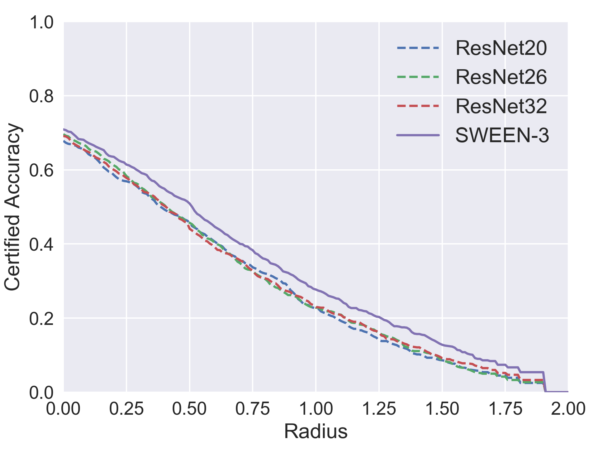
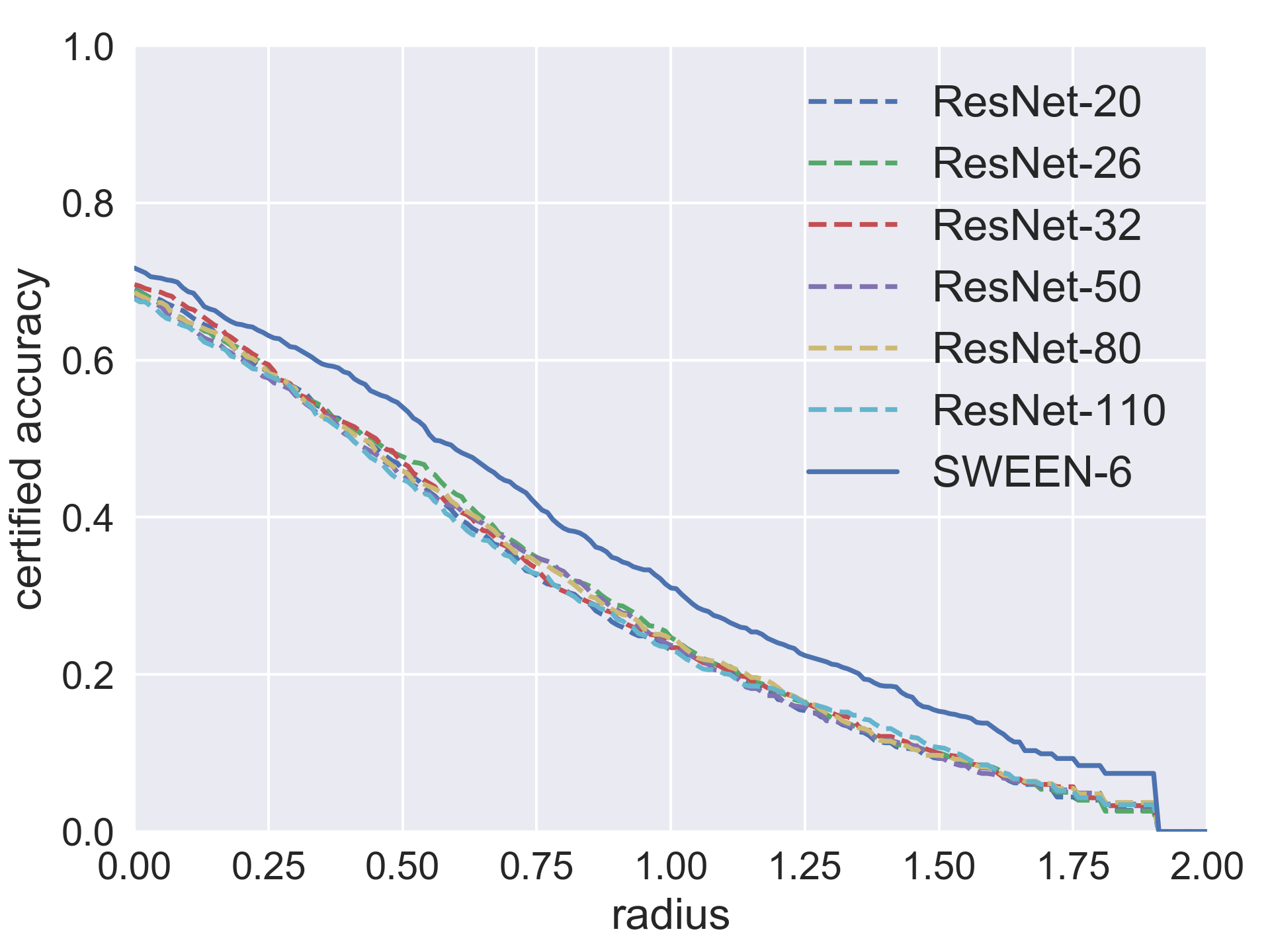
Figure 1: Radius-accuracy curves under $\sigma=0.50$. All models are trained via the standard training. (Left) The SWEEN-3 model and all its candidate models. (Right) The SWEEN-6 model and all its candidate models.

The results show that SWEEN models significantly boost the performance compared to their corresponding candidate models. According to Figure 1, the SWEEN-6 model consistently outperforms all its candidates in terms of the ACA at all radii. The ACR of the SWEEN-6 model is 0.680, much higher than that of the upper envelope of the candidates, which is 0.574. It confirms our theoretical analysis in Section 4 that SWEEN can combine the strength of candidate models and attain superior performance. Besides, SWEEN is effective when only limited numbers of small candidate models are available. The SWEEN-3 model using ResNet-20, ResNet-26, and ResNet-32 achieves higher ACA than the ResNet-110 at all radii on all noise levels. The total training time and the number of parameters of the SWEEN-3 model are 36 % and 30% less than those of ResNet-110, respectively. The improvements can be further amplified by increasing the number and size of candidate models. As an instance, the ACR of the SWEEN-6 model is at least 13% higher than that of the ResNet-110 in Table 1. The above results verify the effectiveness of SWEEN for randomized smoothing.

Table 2: Training time, #parameters and #FLOPs for models under $\sigma=0.50$ via MACER training. All the experiments are run on a single NVIDIA 1080 Ti GPU.

Model	Total hrs	#parameters	#FLOPs
ResNet-110	49.4	1.73M	255.27M
ResNet-20	8.8	0.27M	41.21M
ResNet-26	11.3	0.36M	55.48M
ResNet-32	13.8	0.46M	69.75M
Weight	0.025	-	-
Ensemble	33.9	1.10M	166.44M

Table 3: ACA (%) and ACR on CIFAR-10. All models are trained via MACER training. UE stands for the upper envelope of candidate models.

$\sigma$	Model	0.00	0.25	0.50	0.75	1.00	1.25	1.50	1.75	2.00	ACR
0.25	ResNet-110	81	71	59	43	0	0	0	0	0	0.556
	UE-3	77.4	66.9	56.8	41.9	0	0	0	0	0	0.529
	SWEEN-3	77.7	68.7	60.3	46.6	0	0	0	0	0	0.558
	UE-6	80.7	69.4	56.6	41.8	0	0	0	0	0	0.540
	SWEEN-6	80.7	71.5	61.3	48.1	0	0	0	0	0	0.578
0.50	ResNet-110	66	60	53	46	38	29	19	12	0	0.726
	UE-3	64.9	57.1	49.7	41.1	34.1	26.2	20.2	11.7	0	0.685
	SWEEN-3	64.7	58.4	51.8	43.9	37.2	29.2	22.8	14.6	0	0.727
	UE-6	65.4	58.5	51.8	44.4	35.8	28.0	19.9	11.3	0	0.701
	SWEEN-6	67.0	60.3	53.2	46.8	38.8	30.3	22.6	14.6	0	0.751
1.00	ResNet-110	45	41	38	35	32	29	25	22	18	0.792
	UE-3	39.4	38.2	35.8	33.4	30.3	27.6	24.5	22.0	19.0	0.793
	SWEEN-3	39.5	37.9	35.8	33.2	30.4	27.5	24.6	22.0	19.1	0.796
	UE-6	39.4	38.2	35.8	33.4	30.3	27.6	24.5	22.3	19.5	0.793
	SWEEN-6	42.7	40.4	38.1	34.6	32.0	29.1	26.4	24.0	20.1	0.816

Table 4: ACA (%) and ACR on ImageNet. All models are trained via standard training.

$\sigma$	Model	0.00	0.25	0.50	0.75	1.00	1.25	1.50	1.75	2.00	ACR
0.25	ResNet-50	66.8	58.2	49.0	38.2	0	0	0	0	0	0.469
	SWEEN-IN	67.8	60.2	51.6	41.6	0	0	0	0	0	0.489
0.50	ResNet-50	56.4	52.4	46.4	42.2	37.8	32.6	28.0	21.4	0	0.726
	SWEEN-IN	56.4	52.4	49.6	45.0	40.8	37.0	31.6	25.2	0	0.781
1.00	ResNet-50	43.6	40.6	37.8	35.4	32.4	28.8	25.8	22.4	19.4	0.863
	SWEEN-IN	44.6	42.0	38.6	36.4	35.0	32.6	29.4	25.6	22.4	0.948

MACER training on CIFAR-10  Since SWEEN is compatible with previous training algorithms, we adopt MACER training for the SWEEN-3 model. The results are summarized in Table 3. For the ACA and ACR of the ResNet-110 model, we use the original numbers from Zhai et al. [2020].

In the results, the SWEEN-3 model achieves comparable results to the ResNet-110 but is more efficient. From Table 2 and 3, the SWEEN-3 model takes 33.9 hours to achieve 0.727 in terms of the ACR for $\sigma=0.5$, using three small and easy-to-train candidates models. Meanwhile, it takes 49.4 hours for the ResNet-110 to achieve similar performance on CIFAR-10. This 32% speed up reveals the efficiency of applying SWEEN to previous training methods. Moreover, the SWEEN-6 models outperform the ResNet-110 model on ACA of most radius levels and on ACR by a large margin. To our best knowledge, it establishes a new state-of-the-art certified robustness on CIFAR-10 under $\ell_{2}$ norm.

Results on ImageNet  Table 4 displays the performance of ResNet-50 and SWEEN-IN under the noise levels $\sigma\in\{0.25,0.50,1.00\}$. We note that the performance of ResNet-50 is also the upper envelope of the three models in SWEEN-IN. We can see that the SWEEN-IN model significantly outperforms its corresponding candidate models, similar to the results on CIFAR-10. The results again confirm the effectiveness of our proposed SWEEN framework.

Table 5: ACA (%) and ACR on CIFAR-10. All candidate models are ResNet-110s trained via the standard training. UE stands for the upper envelope, which shows the largest ACA and ACR among the candidate models. AVG stands for the average ACA or ACR of candidate models.

$\sigma$	Model	0.00	0.25	0.5	0.75	1.00	1.25	1.50	1.75	2.00	ACR
0.25	AVG	79.9	67.2	50.3	33.5	0	0	0	0	0	0.491
	UE	80.4	68.3	52.0	34.6	0	0	0	0	0	0.496
	SWEEN	83.5	73.0	60.4	43.8	0	0	0	0	0	0.572
0.50	AVG	68.4	58.0	46.1	34.5	24.4	16.2	9.7	4.4	0	0.568
	UE	69.7	59.3	47.1	35.7	24.9	17.6	10.8	5.1	0	0.581
	SWEEN	71.3	63.3	53.1	44.0	32.6	22.9	15.8	9.2	0	0.691
1.00	AVG	51.9	45.0	37.8	30.9	24.7	18.7	13.5	9.9	7.1	0.558
	UE	53.0	46.0	38.6	31.8	25.5	19.3	14.1	10.5	7.7	0.566
	SWEEN	54.1	47.3	41.0	34.7	27.6	22.9	16.7	12.2	9.2	0.623

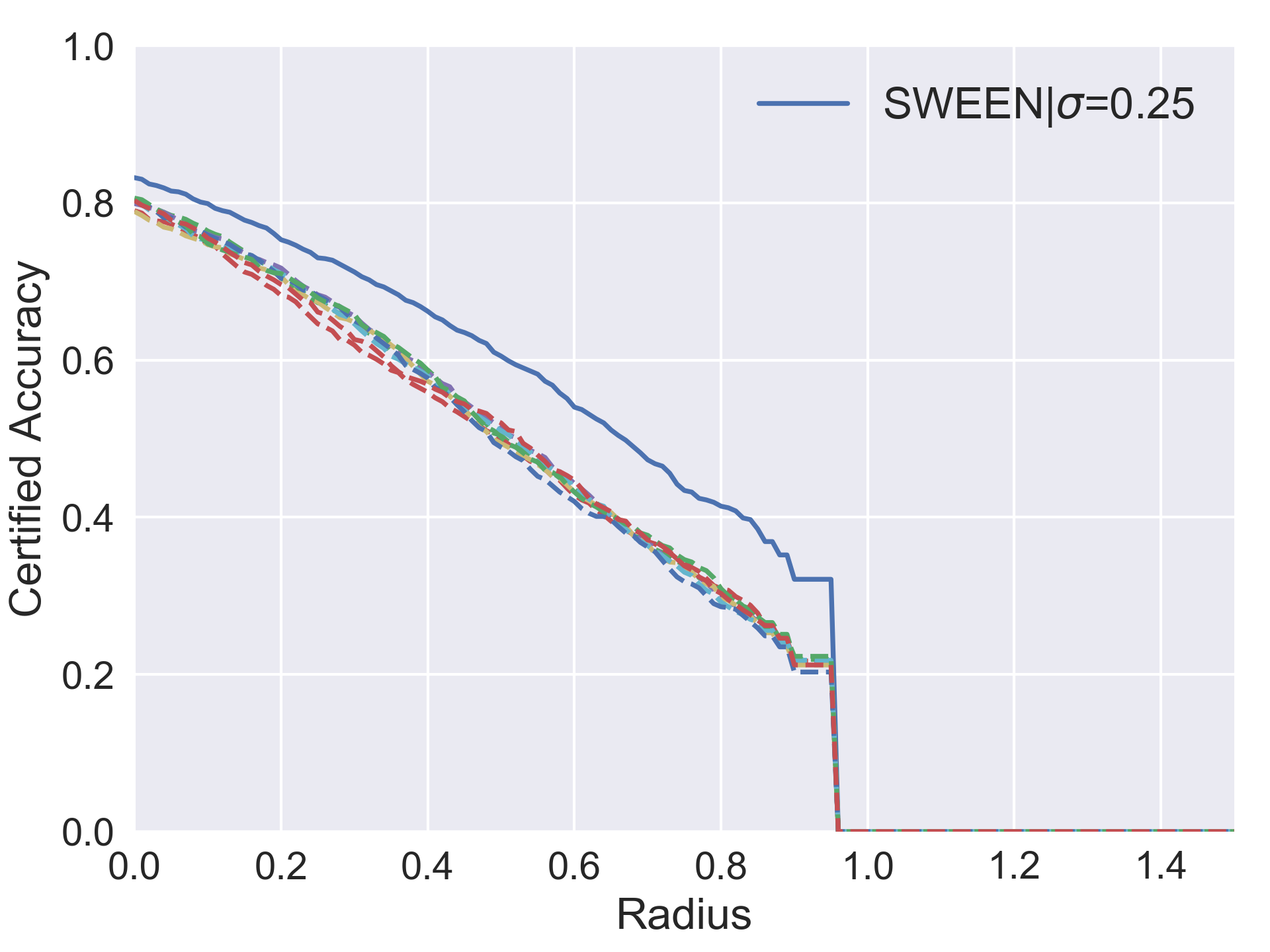
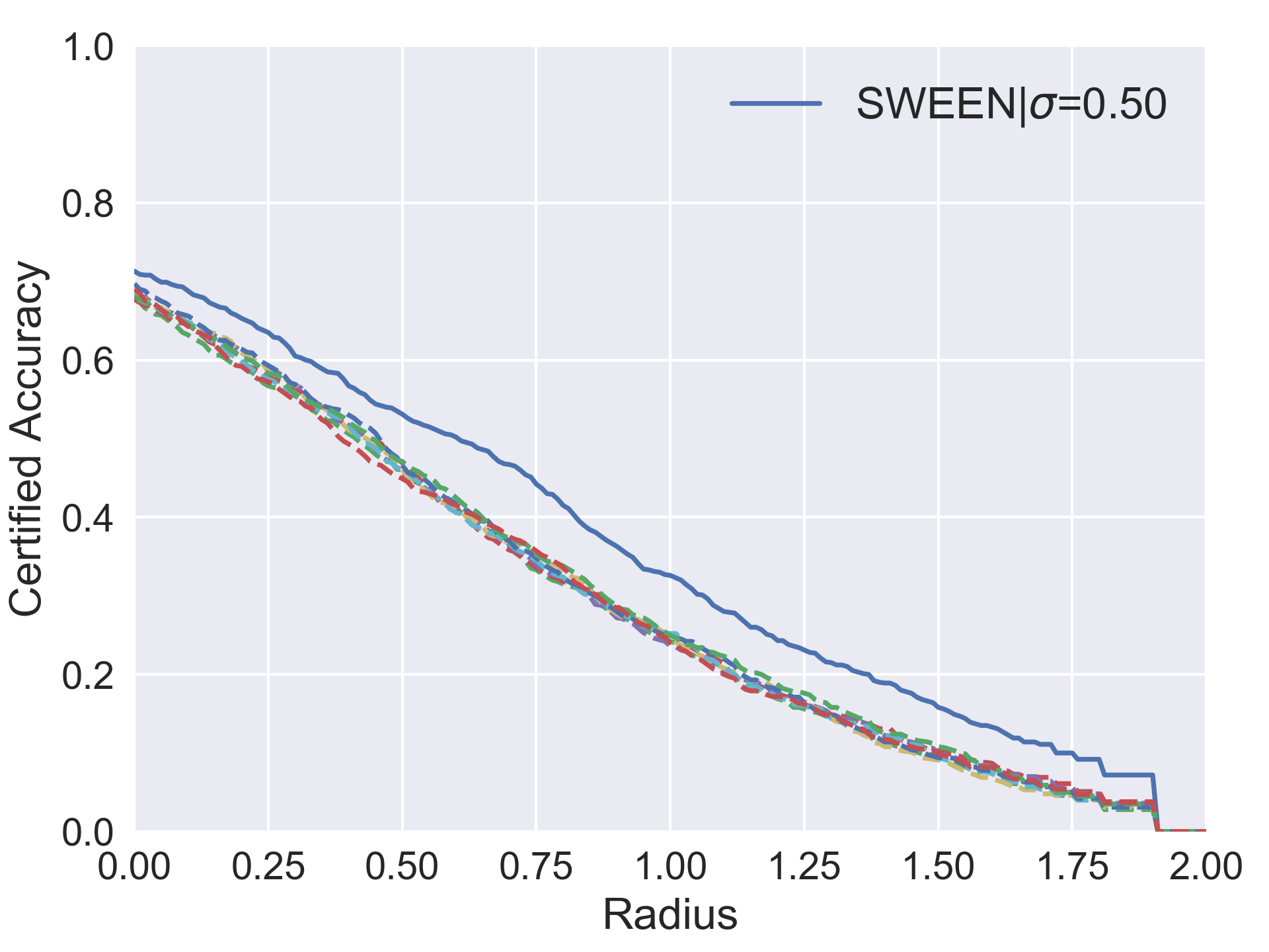
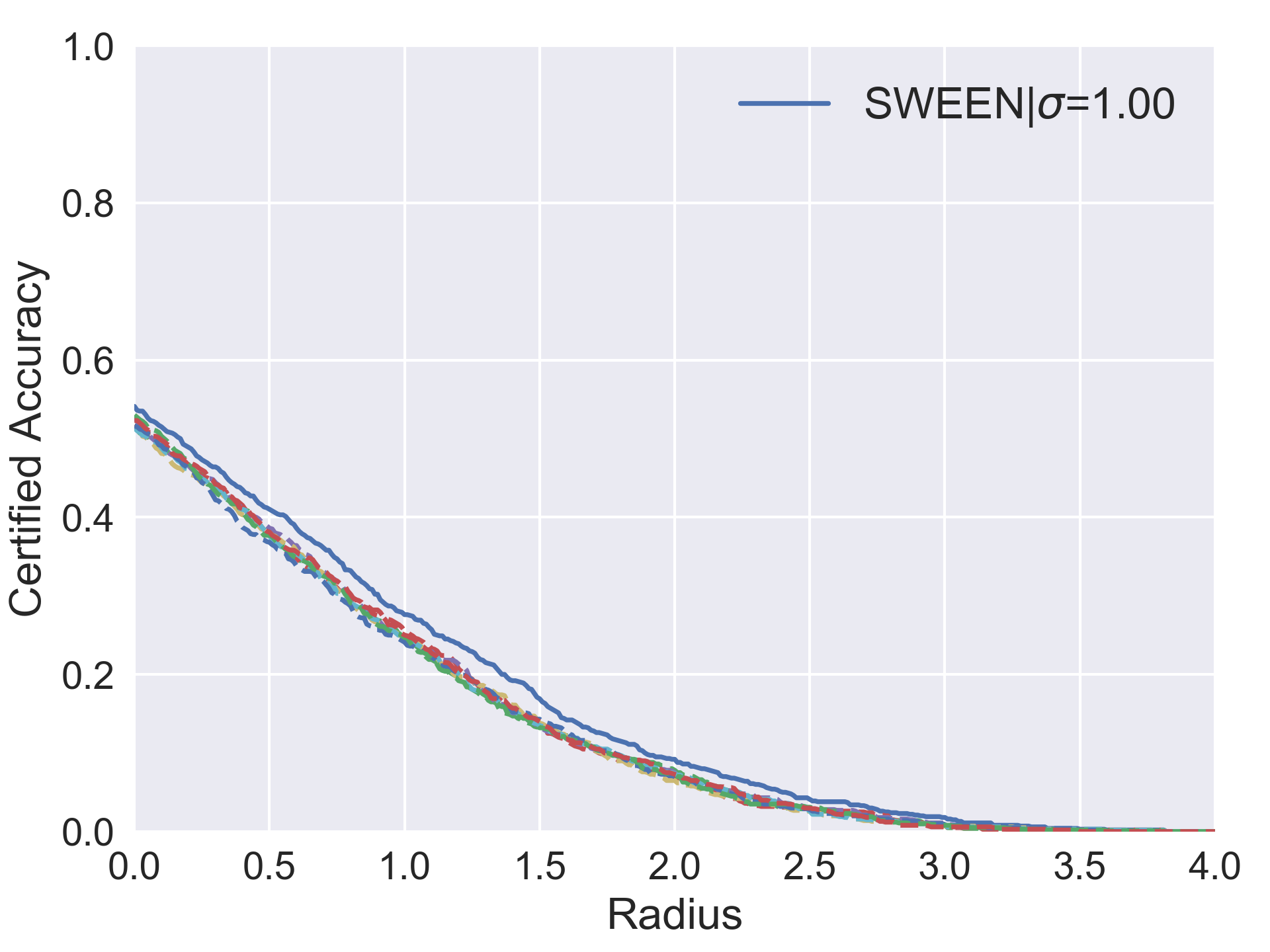
Figure 2: Radius-accuracy curves of SWEEN models and their candidate models. All candidate models are using the ResNet-110 architecture and trained via the standard training. (Left) $\sigma=0.25$. (Middle) $\sigma=0.50$. (Right) $\sigma=1.00$.

Table 6: ACA (%) and ACR on ImageNet. All candidate models are ResNet-50s trained via the standard training. The SWEEN model here contains 3 ResNet-50s. UE stands for the upper envelope, which shows the largest ACA and ACR among the candidate models. AVG stands for the average ACA or ACR of candidate models.

$\sigma$	Model	0.00	0.25	0.5	0.75	1.00	1.25	1.50	1.75	2.00	ACR
0.50	AVG	56.8	52.1	46.1	42.3	37.5	32.8	28.1	21.6	0	0.723
	UE	57.2	52.4	46.4	42.4	37.8	33.0	28.2	21.8	0	0.727
	SWEEN	60.0	55.2	50.2	46.0	42.6	37.8	33.2	28.4	0	0.816

Table 7: ACA (%) and ACR on CIFAR-10. All models are trained via the standard training.

$\sigma$	Model	ACR	#evals/img
0.25	Normal	0.560	600,600
	Adaptive	0.547	246,981
0.50	Normal	0.680	600,600
	Adaptive	0.672	349,805
1.00	Normal	0.626	600,600
	Adaptive	0.624	431,148

SWEEN models using candidates with identical architectures  The SWEEN-3 and SWEEN-6 models are all using candidate models with diverse architectures. For a more comprehensive result, we also experiment with SWEEN models using candidates with identical architectures. For $\sigma\in\{0.25,0.5,1.0\}$, We train 8 ResNet-110 models using different random seeds on CIFAR-10 via the standard training. We then use these models to ensemble SWEEN models.

The results are shown in Table 5 and Figure 2. We can see that SWEEN is still effective in this scenario and significantly boosts the performance compared to candidate models.

We also run experiments on ImageNet using models with identical structure but with different random initialization. We train 3 ResNet-50 on ImageNet via the standard training to ensemble the SWEEN models. Table 6 shows the results. The improvement of SWEEN is substantial compared with the AVG and UE results.

Adaptive prediction ensembling  To alleviate the higher execution cost introduced by SWEEN, we apply the previously mentioned adaptive prediction algorithm to speed up the certification. Experiments are conducted on the SWEEN-6 models via the standard training on CIFAR-10 and the results are summarized in Table 7. It can be observed that the adaptive prediction successfully reduce the number of evaluations. However, the performance of the adaptive prediction models is only slightly worse than their vanilla counterparts.

Other experimental results  Due to space constraints, we only report the main results here. The results of further experiments can be found in Appendix C.

6 Conclusions

In this work, we introduced the smoothed weighted ensembling (SWEEN) to improve randomized smoothed classifiers in terms of both accuracy and robustness. We showed that SWEEN can achieve optimal certified robustness w.r.t. our defined $\gamma$-robustness index. Furthermore, we can obtain the optimal SWEEN model w.r.t. a surrogate loss from training under mild assumptions. We also developed an adaptive prediction algorithm to accelerate the prediction and certification process. Our extensive experiments showed that a properly designed SWEEN model was able to outperform all its candidate models by a significant margin consistently. We also achieve the state-of-the-art certified robustness on CIFAR-10. Moreover, SWEEN models using a few small and easy-to-train candidates could match or exceed a large individual model on performance with a notable reduction in total training time. Our theoretical and empirical results confirmed that SWEEN is a viable tool for improving the performance of randomized smoothing models.

Appendix A Proofs

A.1 Proof of Lemma 1

Define

$$\begin{split}\mathscr{F}^{\prime}_{p}&=\left\{\phi(x)=\int_{\Theta}w(\theta)g(x;\theta)d\theta\Big{|}\right.\\ &\|\phi\|_{p}<\infty,w(\theta)\geq 0\bigg{\}},\end{split}$$ (14)

$$\hat{\mathscr{F}}^{\prime}_{\theta}=\left\{\phi(x)=\sum_{k=1}^{K}w_{k}g(x;\theta_{k})\Big{|}w_{k}\geq 0\right\}.$$ (15)

We have $\mathscr{F}_{p}\subseteq\mathscr{F}^{\prime}_{p},\hat{\mathscr{F}}_{\theta}\subseteq\hat{\mathscr{F}}^{\prime}_{\theta}$.

Lemma 2.

Let $\mu$ be any probability measure on $\mathbb{R}^{d}$. For $\phi:\mathbb{R}^{d}\to\mathbb{R}^{M}$, define the norm $\|\phi\|_{\mu}^{2}\triangleq\int_{\mathbb{R}^{d}}\|\phi(x)\|_{2}^{2}d\mu(x)$. Fix $\phi\in\mathscr{F}^{\prime}_{p}$, then for any $\eta>0$, with probability at least $1-\eta$ over $\theta_{1},...,\theta_{K}$ drawn i.i.d. from $p$, there exists $\hat{\phi}(x)=\sum\limits_{k=1}^{K}c_{k}g(x;\theta_{k})\in\hat{\mathscr{F}}^{\prime}_{\theta}$ which satisfies

$$\|\hat{\phi}-\phi\|_{\mu}\leq\frac{\|\phi\|_{p}}{\sqrt{K}}(1+\sqrt{2\log\frac{1}{\eta}}).$$ (16)

Proof.

Sine $\phi\in\mathscr{F}^{\prime}_{p}$, we can write $\phi(x)=\int_{\Theta}w(\theta)g(x;\theta)d\theta$, where $w(\theta)\geq 0$. Construct $\phi_{k}=\beta_{k}g(\cdot;\theta_{k}),k=1,2,\cdots,K$, where $\beta_{k}=\frac{w(\theta_{k})}{p(\theta_{k})}$, then $\mathbb{E}\phi_{k}=\phi,\|\phi_{k}\|_{\mu}=\sqrt{\int_{\mathbb{R}^{d}}\beta_{k}^{2}\|g(x;\theta_{k})\|_{2}^{2}d\mu(x)}\leq|\beta_{k}|\leq\|\phi\|_{p}$. We then define

$$u(\theta_{1},\cdots,\theta_{K})=\|\frac{1}{K}\sum_{k=1}^{K}\phi_{k}-\phi\|_{\mu}.$$ (17)

First, by using Jensen’s inequality and the fact that $\|\phi_{k}\|_{\mu}\leq\|\phi\|_{p}$, we have

$$\mathbb{E}[u(\theta)] \leq \sqrt{\mathbb{E}[u^{2}(\theta)]}$$

$$= \sqrt{\mathbb{E}[\|\frac{1}{K}\sum_{k=1}^{K}\phi_{k}-\mathbb{E}\phi_{k}\|_{\mu}^{2}]}$$

$$= \sqrt{\frac{1}{K}(\mathbb{E}\|\phi_{k}\|_{\mu}^{2}-\|\mathbb{E}\phi_{k}\|_{\mu}^{2})}\leq\frac{\|\phi\|_{p}}{\sqrt{K}}.$$

Next, for $\theta_{1},\cdots,\theta_{M}$ and $\tilde{\theta}_{i}$, we have

$$|u(\theta_{1},\cdots,\theta_{M})-u(\theta_{1},\cdots,\tilde{\theta}_{i},\cdots,\theta_{M})|$$

$$= |\|\frac{1}{K}\sum_{k=1}^{K}\phi_{k}-\phi\|_{\mu}-\|\frac{1}{K}(\sum_{k=1,k\neq i}^{K}\phi_{k}+\tilde{\phi}_{i})-\phi\|_{\mu}|$$

$$\leq \|\frac{1}{K}\sum_{k=1}^{M}\phi_{k}-\frac{1}{K}(\sum_{k=1,k\neq i}^{M}\phi_{k}+\tilde{\phi}_{i})\|_{\mu}$$

$$= \frac{\|\phi_{i}-\tilde{\phi}_{i}\|_{\mu}}{K}$$

$$\leq \frac{2\|\phi\|_{p}}{K}.$$

Now we can use McDiarmid’s inequality to bound $u(\theta)$, which gives

$$\begin{split}\mathbb{P}[u(\theta)-\frac{\|\phi\|_{p}}{\sqrt{K}}\geq\varepsilon]&\leq\mathbb{P}[u(\theta)-\mathbb{E}u(\theta)\geq\varepsilon]\\ &\leq\exp(-\frac{K\varepsilon^{2}}{2\|\phi\|_{p}^{2}}).\end{split}$$ (18)

The theorem follows by setting $\delta$ to the right hand side and solving $\varepsilon$.

∎

Lemma 3.

Let $\mu$ be any probability measure on $\mathbb{R}^{d}$. For $\phi:\mathbb{R}^{d}\to\mathbb{R}^{M}$, define the norm $\|\phi\|_{\mu}^{2}\triangleq\int_{\mathbb{R}^{d}}\|\phi(x)\|_{2}^{2}d\mu(x)$, then for any $\eta>0$, for $K\geq M\|\phi\|_{p}^{2}(1+\sqrt{2\log\frac{1}{\eta}})^{2}$, with probability at least $1-\eta$ over $\theta_{1},...,\theta_{K}$ drawn i.i.d. from $p$, there exists $\hat{\phi}(x)=\sum\limits_{k=1}^{K}c_{k}g(x;\theta_{k})\in\hat{\mathscr{F}}_{\theta}$ which satisfies

$$\|\hat{\phi}-\phi\|_{\mu}<2\sqrt{\|\phi\|_{p}}\sqrt[4]{\frac{M}{K}}(1+\sqrt{2\log\frac{1}{\eta}})^{\frac{1}{2}}.$$ (19)

Proof.

Fix $\phi\in\mathscr{F}_{p}\subseteq\mathscr{F}^{\prime}_{p}$, by using Lemma 2, we have that for any $\delta>0$, with probability at least $1-\eta$ over $\theta_{1},...,\theta_{K}$ drawn i.i.d. from $p$, there exists $\tilde{\phi}(x)=\sum\limits_{k=1}^{K}c_{k}g(x;\theta_{k})\in\hat{\mathscr{F}}^{\prime}_{\theta}$ which satisfies

$$\|\tilde{\phi}-\phi\|_{\mu}<\frac{\|\phi\|_{p}}{\sqrt{K}}(1+\sqrt{2\log\frac{1}{\eta}})\triangleq B(K).$$ (20)

Denote $C=\sum\limits_{k=1}^{K}c_{k}$, and define $s(t)\triangleq\sum\limits_{i=1}^{M}t_{i}$ as the sum of all elements of $t\in\mathbb{R}^{M}$. Then $s(g(x;\theta))=1,\forall x\in\mathbb{R}^{d},\theta\in\Theta$. Thus,

$$s(\phi(x)) = \sum\limits_{i=1}^{M}\phi_{i}(x)=\sum\limits_{i=1}^{M}\int_{\Theta}w(\theta)g_{i}(x;\theta)d\theta$$

$$= \int_{\Theta}w(\theta)\sum\limits_{i=1}^{M}g_{i}(x;\theta)d\theta=\int_{\Theta}w(\theta)d\theta=1,$$

$$s(\tilde{\phi}(x)) = \sum\limits_{i=1}^{M}\tilde{\phi}_{i}(x)=\sum\limits_{i=1}^{M}\sum\limits_{k=1}^{K}c_{k}g_{i}(x;\theta_{k})$$

$$= \sum\limits_{k=1}^{K}c_{k}\sum\limits_{i=1}^{M}g_{i}(x;\theta_{k})=\sum\limits_{k=1}^{K}c_{k}=C.$$

Now we have

$$B(K)^{2}>\|\tilde{\phi}-\phi\|^{2}_{\mu} = \int_{\mathbb{R}^{d}}\|\tilde{\phi}(x)-\phi(x)\|_{2}^{2}d\mu(x)$$

$$\geq \int_{\mathbb{R}^{d}}\frac{(s(\tilde{\phi}(x)-\phi(x)))^{2}}{M}d\mu(x)$$

$$= \int_{\mathbb{R}^{d}}\frac{(C-1)^{2}}{M}d\mu(x)$$

$$= \frac{(C-1)^{2}}{M},$$

which gives $1-\sqrt{M}B(K)<C<1+\sqrt{M}B(K)$. Construct $\hat{\phi}(x)=\frac{\tilde{\phi}(x)}{C}$, then $\hat{\phi}\in\hat{\mathscr{F}}_{\theta}$ and

$$\|\hat{\phi}-\phi\|^{2}_{\mu}$$

$$= \int_{\mathbb{R}^{d}}\|\hat{\phi}(x)-\phi(x)\|_{2}^{2}d\mu(x)$$

$$= \int_{\mathbb{R}^{d}}\|C^{-1}\tilde{\phi}(x)-\phi(x)||_{2}^{2}d\mu(x)$$

$$= \int_{\mathbb{R}^{d}}\|(\tilde{\phi}(x)-\phi(x))+(C^{-1}-1)\tilde{\phi}(x)\|_{2}^{2}d\mu(x)$$

$$= \int_{\mathbb{R}^{d}}(\|\tilde{\phi}(x)-\phi(x)\|^{2}_{2}+\|(C^{-1}-1)\tilde{\phi}(x)\|_{2}^{2}$$

$$+2(C^{-1}-1)\langle\tilde{\phi}(x)-\phi(x),\tilde{\phi}(x)\rangle)d\mu(x)$$

$$= \int_{\mathbb{R}^{d}}(\|\hat{\phi}(x)-\phi(x)\|^{2}_{2}+(C^{-2}-1)\|\tilde{\phi}(x)\|_{2}^{2}$$

$$+2(1-C^{-1})\langle\phi(x),\tilde{\phi}(x)\rangle)d\mu(x).$$

Since we have $\frac{C^{2}}{M}\leq\|\tilde{\phi}(x)\|_{2}^{2}\leq C^{2},\ |\langle\phi(x),\tilde{\phi}(x)\rangle|\leq\sqrt{\|\phi(x)\|_{2}^{2}\|\tilde{\phi}(x)\|_{2}^{2}}\leq C$, it holds that

(i) When $1<C<1+\sqrt{M}B(K)$,

$$\|\hat{\phi}-\phi\|^{2}_{\mu}$$

$$\leq \int_{\mathbb{R}^{d}}(\|\tilde{\phi}(x)-\phi(x)\|^{2}_{2}+\frac{1-C^{2}}{M}+2(C-1))d\mu(x)$$

$$\leq B(K)^{2}+\frac{1-C^{2}}{M}+2(C-1)$$

$$\leq -\frac{2B(K)}{\sqrt{M}}+2\sqrt{M}B(K);$$

(ii) When $1-\sqrt{M}B(K)<C\leq 1$,

$$\|\hat{\phi}-\phi\|^{2}_{\mu}$$

$$\leq \int_{\mathbb{R}^{d}}(\|\tilde{\phi}(x)-\phi(x)\|^{2}_{2}+(1-C^{2})+2(1-C))d\mu(x)$$

$$\leq B(K)^{2}+4-(1+C)^{2}$$

$$\leq 4\sqrt{M}B(K)-(M-1)B(K)^{2}$$

$$< 4\sqrt{M}B(K).$$

Thus, with probability at least $1-\eta$ over $\theta_{1},...,\theta_{K}$ drawn i.i.d. from $p$,

$$\|\hat{\phi}-\phi\|_{\mu}<2\sqrt{\sqrt{M}B(K)}=2\sqrt{\|\phi\|_{p}}\sqrt[4]{\frac{M}{K}}(1+\sqrt{2\log\frac{1}{\eta}})^{\frac{1}{2}}.$$

∎

Lemma 4.

Suppose $l(\cdot,\cdot)$ is $L$-Lipschitz in its first argument. Fix $\phi\in\mathscr{F}_{p}$, then for any $\eta>0$, for $K\geq M\|\phi\|_{p}^{2}(1+\sqrt{2\log\frac{1}{\eta}})^{2}$, with probability at least $1-\eta$ over $\theta_{1},...,\theta_{K}$ drawn i.i.d. from $p$, there exists $\hat{\phi}\in\hat{\mathscr{F}}_{\theta}$ which satisfies

$$|\mathbb{E}_{(x,y)\sim\mathcal{D}}[l(\hat{\phi}(x),y)]-\mathbb{E}_{(x,y)\sim\mathcal{D}}[l(\phi(x),y)]|$$

$$<2L\sqrt{\|\phi\|_{p}}\sqrt[4]{\frac{M}{K}}(1+\sqrt{2\log\frac{1}{\eta}})^{\frac{1}{2}}.$$

Proof.

$$|\mathbb{E}[l(\hat{\phi}(x),y)]-\mathbb{E}[l(\phi(x),y)]|$$

$$\leq \mathbb{E}|c(\phi(x),y)-c(\hat{\phi}(x),y)|$$

$$\leq L\mathbb{E}\|\phi(x)-\hat{\phi}(x)\|_{2}$$

$$\leq L\sqrt{\mathbb{E}\|\phi(x)-\hat{\phi}(x)\|^{2}_{2}}$$

$$= L\|\phi-\hat{\phi}\|_{\mathcal{D}|_{x}}$$

The desired result follows from Lemma 3. ∎

Lemma 5.

(Corollary of Proposition 1 in Zhai et al. [2020]) Given any $p_{1},p_{2},\cdots,p_{M}$ satisfies $p_{1}\geq p_{2}\geq\cdots\geq p_{M}\geq 0$ and $p_{1}+p_{2}+\cdots+p_{M}=1$. The derivative of $\mathrm{clip}(\frac{\sigma}{2}[\Phi^{-1}(p_{1})-\Phi^{-1}(p_{2})];0,D)$ with respect to $p_{1}$ and $p_{2}$ is bounded.

Now we can prove Lemma 1.

Proof of Lemma 1. Let $\phi_{0}\in\mathscr{F}_{p}$ such that $\mathcal{I}_{\gamma}(\phi_{0})>\sup_{\phi\in\mathscr{F}_{p}}\mathcal{I}_{\gamma}(\phi)-\frac{\varepsilon}{2}$. From Lemma 5 we know that $q(p,y)\triangleq\mathrm{clip}(\frac{\sigma}{2}[\Phi^{-1}(p_{y})-\Phi^{-1}(\max_{k\neq y}p_{k})];0,D)$ is Lipschitz in its first argument. Since $m$ is Lipschitz, $c(p,y)\triangleq m(q(p,y))$ is also Lipschitz in its first argument with some constant $L$. Apply Lemma 4, we have that for $K\geq M\|\phi\|_{p}^{2}(1+\sqrt{1+2\log\frac{1}{\delta}})^{2}$, with probability at least $1-\eta$ over $\theta_{1},...,\theta_{K}$ drawn i.i.d. from $p$, there exists $\hat{\phi}\in\hat{\mathscr{F}}_{\theta}$ which satisfies

$$\mathcal{I}_{\gamma}(\phi_{0})-\mathcal{I}_{\gamma}(\hat{\phi})$$

$$= \mathbb{E}_{(x,y)\sim\mathcal{D}}[l(\phi_{0}(x),y)]-\mathbb{E}_{(x,y)\sim\mathcal{D}}[l(\hat{\phi}(x),y)]$$

$$< 2L\sqrt{\|\phi_{0}\|_{p}}\sqrt[4]{\frac{M}{K}}(1+\sqrt{2\log\frac{1}{\eta}})^{\frac{1}{2}}.$$

When $K>\frac{256L^{4}\|\phi_{0}\|^{2}_{p}M(1+\sqrt{2\log\frac{1}{\eta}})^{2}}{\varepsilon^{4}}$, we have

$$\sup_{\phi\in\mathscr{F}_{p}}\mathcal{I}_{\gamma}(\phi)-\mathcal{I}_{\gamma}(\hat{\phi})$$

$$= (\sup_{\phi\in\mathscr{F}_{p}}\mathcal{I}_{\gamma}(\phi)-\mathcal{I}_{\gamma}(\phi_{0}))+(\mathcal{I}_{\gamma}(\phi_{0})-\mathcal{I}_{\gamma}(\hat{\phi}))$$

$$< \frac{\varepsilon}{2}+\frac{\varepsilon}{2}=\varepsilon.$$

If $\mathcal{I}_{\gamma}(\phi_{0})=\sup_{\phi\in\mathscr{F}_{p}}\mathcal{I}_{\gamma}(\phi)$, which means $\|\phi_{0}\|_{p}$ is independent of $\varepsilon$, $K=O(\frac{1}{\varepsilon^{4}})$.∎

A.2 Proof of Theorem 2

First we introduce some results from statistical learning theory.

Definition 3.

(Gaussian complexity). Let $\mu$ be a probability distribution on a set $\mathcal{X}$ and suppose that $x_{1},...,x_{n}$ are independent samples selected according to $\mu$. Let $\mathscr{F}$ be a class of functions mapping from $X$ to $\mathbb{R}$. The Gaussian complexity of $\mathscr{F}$ is

$$G_{n}[\mathscr{F}]\triangleq\mathbb{E}[\sup_{f\in\mathscr{F}}|\frac{2}{n}\sum\limits_{i=1}^{n}\xi_{i}f(x_{i})|\big{|}x_{1},...,x_{n};\xi_{i},...,\xi_{n}]$$

where $\xi_{1},...,\xi_{n}$ are independent $\mathcal{N}(0,1)$ random variables.

Definition 4.

(Rademacher complexity) Let $\mu$ be a probability distribution on a set $\mathcal{X}$ and suppose that $x_{1},...,x_{n}$ are independent samples selected according to $\mu$. Let $\mathscr{F}$ be a class of functions mapping from $X$ to $\mathbb{R}$. The Rademacher complexity of $\mathscr{F}$ is

$$R_{n}[\mathscr{F}]\triangleq\mathbb{E}[\sup_{f\in\mathscr{F}}|\frac{2}{n}\sum\limits_{i=1}^{n}\sigma_{i}f(x_{i})|\big{|}x_{1},...,x_{n};\sigma_{i},...,\sigma_{n}]$$

where $\sigma_{1},...,\sigma_{n}$ are independent uniform $\{\pm 1\}$-valued random variables.

Lemma 6.

(Part of Lemma 4 in Bartlett and Mendelson [2001]). There are absolute constants $\beta$ such that for every class $\mathscr{F}$ and every integer $n$, $R_{n}(\mathscr{F})\leq\beta G_{n}(\mathscr{F})$.

Lemma 7.

(Corollary of Theorem 8 in Bartlett and Mendelson [2001]). Consider a loss function $c:\mathcal{A}\times Y\to[0,1]$. Let $\mathscr{F}$ be a class of functions mapping from $\mathcal{X}$ to $\mathcal{A}$ and let $(x_{i},y_{i})_{i=1}^{n}$ be independently selected according to the probability measure $\mu$. Then, for any integer $n$ and any $0<\eta<1$, with probability at least $1-\eta$ over samples of length $n$, every $f$ in $\mathscr{F}$ satisfies

$$\mathbb{E}_{(x,y)\sim\mu}[c(f(x),y)]$$

$$\leq \frac{1}{n}\sum_{i=1}^{n}c(f(x_{i}),y_{i})+R_{n}[\tilde{c}\circ\mathscr{F}]+\sqrt{\frac{8\log\frac{2}{\eta}}{n}},$$

where $\tilde{c}\circ\mathscr{F}=\{(x,y)\mapsto c(f(x),y)-c(0,y)\big{|}f\in\mathscr{F}\}$

Lemma 8.

(Corollary of Theorem 14 in Bartlett and Mendelson [2001]). Let $\mathcal{A}=\mathbb{R}^{M}$ and let $\mathscr{F}$ be a class of functions mapping from $\mathcal{X}$ to $\mathcal{A}$. Suppose that there are real-valued classes $\mathscr{F}_{1},...,\mathscr{F}_{M}$ such that $\mathscr{F}$ is a subset of their Cartesian product. Assume further that $c:\mathcal{A}\times Y\to\mathbb{R}$ is such that, for all $y\in Y$, $c(\cdot,y)$ is a Lipschitz function with constant $L$ which passes through the origin and is uniformly bounded. Then

$$G_{n}(c\circ\mathscr{F})\leq 2L\sum_{i=1}^{M}G_{n}(\mathscr{F}_{i}).$$

Now we prove the following lemma:

Lemma 9.

Let $c,\mathscr{F},(x_{i},y_{i})_{i=1}^{n},\tilde{c}\circ\mathscr{F}$ be as in Lemma 7. Then, for any integer $n$ and any $0<\eta<1$, with probability at least $1-\eta$ over samples of length $n$, every $f$ in $\mathscr{F}$ satisfies

$$\frac{1}{n}\sum_{i=1}^{n}c(f(x_{i}),y_{i})$$

$$\leq \mathbb{E}_{(x,y)\sim\mu}[c(f(x),y)]+R_{n}[\tilde{c}\circ\mathscr{F}]+\sqrt{\frac{8\log\frac{2}{\eta}}{n}}.$$

Proof.

$$\frac{1}{n}\sum_{i=1}^{n}c(f(x_{i}),y_{i})-\mathbb{E}_{(x,y)\sim\mu}[c(f(x),y)]$$

$$\leq \sup_{h\in c\circ\mathscr{F}}(\hat{\mathbb{E}}_{n}h-\mathbb{E}h)$$

$$= \sup_{h\in\tilde{c}\circ\mathscr{F}}(\hat{\mathbb{E}}_{n}h-\mathbb{E}h)+\hat{\mathbb{E}}_{n}c(0,y)-\mathbb{E}c(0,y).$$

When an $(x_{i},y_{i})$ pair changes, the random variable $\sup\limits_{h\in\tilde{c}\circ\mathscr{F}}(\hat{\mathbb{E}}_{n}h-\mathbb{E}h)$ can change by no more than $\frac{2}{n}$. McDiarmid’s inequality implies that with probability at least $1-\frac{\eta}{2}$,

$$\sup\limits_{h\in\tilde{c}\circ\mathscr{F}}(\hat{\mathbb{E}}_{n}h-\mathbb{E}h)\leq\mathbb{E}\sup\limits_{h\in\tilde{c}\circ\mathscr{F}}(\hat{\mathbb{E}}_{n}h-\mathbb{E}h)+\sqrt{\frac{2\log\frac{2}{\eta}}{n}}.$$

A similar argument, together with the fact that $\mathbb{E}\hat{\mathbb{E}}_{n}c(0,y)=\mathbb{E}c(0,y)$, shows that with probability at least $1-\eta$,

$$\mathbb{R}_{emp}[f]\leq\mathbb{R}[f]+\mathbb{E}\sup\limits_{h\in\tilde{c}\circ\mathscr{F}}(\hat{\mathbb{E}}_{n}h-\mathbb{E}h)+\sqrt{\frac{8\log\frac{2}{\eta}}{n}}.$$

It’s left to show that $\mathbb{E}\sup\limits_{h\in\tilde{c}\circ\mathscr{F}}(\hat{\mathbb{E}}_{n}h-\mathbb{E}h)\leq\mathcal{R}_{n}[\tilde{c}\circ\mathscr{F}]$. Let $(x^{\prime}_{1},y^{\prime}_{1}),...,(x^{\prime}_{n},y^{\prime}_{n})$ be drawn i.i.d. from $\mu$ and independent from $(x_{i},y_{i})_{i=1}^{n}$, then

$$\mathbb{E}\sup\limits_{h\in\tilde{c}\circ\mathscr{F}}(\hat{\mathbb{E}}_{n}h-\mathbb{E}h)$$

$$= \mathbb{E}\sup\limits_{h\in\tilde{c}\circ\mathscr{F}}\mathbb{E}[\hat{\mathbb{E}}_{n}h-\frac{1}{n}\sum_{i=1}^{n}h(x^{\prime}_{i},y^{\prime}_{i})]$$

$$\leq \mathbb{E}\mathbb{E}\sup\limits_{h\in\tilde{c}\circ\mathscr{F}}[\hat{\mathbb{E}}_{n}h-\frac{1}{n}\sum_{i=1}^{n}h(x^{\prime}_{i},y^{\prime}_{i})]$$

$$= \mathbb{E}\sup\limits_{h\in\tilde{c}\circ\mathscr{F}}\frac{1}{n}(\sum_{i=1}^{n}h(x_{i},y_{i})-\sum_{i=1}^{n}h(x^{\prime}_{i},y^{\prime}_{i}))$$

$$\leq 2\mathbb{E}\sup\limits_{h\in\tilde{c}\circ\mathscr{F}}\frac{1}{n}\sum_{i=1}^{n}\sigma_{i}h(x_{i},y_{i})$$

$$\leq \mathcal{R}_{n}[\tilde{c}\circ\mathscr{F}].$$

∎

We can prove the following result:

Theorem 3.

Let $\mathcal{A}=\mathbb{R}^{M}$ and let $\mathscr{F}$ be a class of functions mapping from $\mathcal{X}$ to $\mathcal{A}$. Suppose that there are real-valued classes $\mathscr{F}_{1},...,\mathscr{F}_{M}$ such that $\mathscr{F}$ is a subset of their Cartesian product. Assume further that the loss function $c:\mathcal{A}\times Y\to\mathbb{R}$ is such that, for all $y\in Y$, $c(\cdot,y)$ is a Lipschitz function with constant $L$ and is uniformly bounded. Let $\{(x_{i},y_{i})\}_{i=1}^{n}$ be independently selected according to the probability measure $\mu$. Then, for any integer $n$ and any $0<\eta<1$, there is a probability of at least $1-\eta$ that every $f\in\mathscr{F}$ has

$$|\frac{1}{n}\sum_{i=1}^{n}c(f(x_{i}),y_{i})-\mathbb{E}_{(x,y)\sim\mu}[c(f(x),y)]|$$

$$\leq\beta L\sum_{j=1}^{M}G_{n}[\mathscr{F}_{j}]+\sqrt{\frac{8\log\frac{4}{\eta}}{n}},$$

where $\beta$ is a constant.

Proof.

From Lemma 7 and 9 we have that with probability at least $1-\eta$ over samples of length $n$, every $f$ in $\mathscr{F}$ satisfies

$$|\frac{1}{n}\sum_{i=1}^{n}c(f(x_{i}),y_{i})-\mathbb{E}_{(x,y)\sim\mu}[c(f(x),y)]|$$

$$\leq R_{n}[\tilde{c}\circ\mathscr{F}]+\sqrt{\frac{8\log\frac{4}{\eta}}{n}},$$

it follows by applying Lemma 6 and 8. ∎

Lemma 10.

Let $c(\cdot,\cdot),\beta$ be as in Theorem 3. Let $(x_{i},y_{i})_{i=1}^{n}$ be independently selected according to the probability measure $\mathcal{D}$. For any integer $n$ and any $0<\eta<1$, there is a probability of at least $1-\eta$ that every $f\in\hat{\mathscr{F}}_{\theta}$ has

$$|\frac{1}{n}\sum_{i=1}^{n}c(f(x_{i}),y_{i})-\mathbb{E}_{(x,y)\sim\mathcal{D}}[c(f(x),y)]|$$

$$\leq\frac{2\beta LMK}{\sqrt{n}}+\sqrt{\frac{8\log\frac{4}{\eta}}{n}}.$$

Proof.

Denote

$$\hat{\mathscr{F}}_{\theta}(i)=\bigg{\{}\phi(x)=\sum_{k=1}^{K}w_{k}g_{i}(x;w_{k})\Big{|}$$

$$w_{k}\geq 0,\sum_{k=1}^{K}w_{k}=1\bigg{\}},1\leq i\leq M.$$

We have that $\hat{\mathscr{F}}_{\theta}\subseteq\bigotimes\limits_{k=1}^{M}\hat{\mathscr{F}}_{\theta}(i)$, where $\bigotimes$ stands for a Cartesian product operation. The Gaussian comlexities of $\hat{\mathscr{F}}_{\theta}(i)$’s can be bounded as

$$G_{n}[\hat{\mathscr{F}}_{\theta}(j)] = \mathbb{E}_{x,\xi}[\sup_{\phi\in\hat{\mathscr{F}}_{\theta}(j)}|\frac{2}{n}\sum\limits_{i=1}^{n}\xi_{i}\phi(x_{i})|]$$

$$= \mathbb{E}_{x,\xi}[\sup_{w}|\frac{2}{n}\sum\limits_{i=1}^{n}\xi_{i}\sum\limits_{k=1}^{K}w_{k}g_{j}(x_{i};w_{k})|]$$

$$= \mathbb{E}_{x,\xi}[\sup_{w}|\sum\limits_{k=1}^{K}w_{k}\frac{2}{n}\sum\limits_{i=1}^{n}\xi_{i}g_{j}(x_{i};w_{k})|]$$

$$\leq \mathbb{E}_{x,\xi}[2\sum\limits_{k=1}^{K}|\frac{1}{n}\sum\limits_{i=1}^{n}\xi_{i}g_{j}(x_{i};w_{k})|]$$

$$\leq \mathbb{E}_{x}[2\sum\limits_{k=1}^{K}\sqrt{\mathbb{E}_{g}(\frac{1}{n}\sum\limits_{i=1}^{n}\xi_{i}g_{j}(x_{i};w_{k}))^{2}}]$$

$$= \mathbb{E}_{x}[2\sum\limits_{k=1}^{K}\sqrt{\frac{1}{n^{2}}\sum\limits_{i=1}^{n}g_{j}(x_{i};w_{k})^{2}}]$$

$$\leq \mathbb{E}_{x}[2\sum\limits_{k=1}^{K}\sqrt{\frac{1}{n}}]$$

$$= \frac{2K}{\sqrt{n}}.$$

The desired result follows by applying Theorem 3 to $\hat{\mathscr{F}}_{\theta},\hat{\mathscr{F}}_{\theta}(1),\cdots,\hat{\mathscr{F}}_{\theta}(M)$ and $\mathcal{D}$. ∎

Next, we give the definition of semi-empirical risk. The term ”semi-” implies that it is empirical with respect to the training set but not the smoothing operation.

Definition 5.

(Semi-empirical risk). For a surrogate loss function $l(\cdot,\cdot):\mathbb{R}^{M}\times\mathbb{R}^{M}\to\mathbb{R}$ and training set $\{(x_{i},y_{i})\}_{i=1}^{n}$, the semi-empirical risk of $\phi(x)=\sum_{k=1}^{K}w_{k}g(x;\theta_{k})\in\hat{\mathscr{F}}_{\theta}$ are defined as

$$\mathcal{R}_{se}[\phi] = \frac{1}{n}\sum_{i=1}^{n}l(\sum_{k=1}^{K}w_{k}g(x_{i};\theta_{k}),y_{i}).$$ (21)

We can use Lemma 4 and 10 to prove the following result:

Theorem 4.

Suppose for all $y\in\mathcal{Y}$, $l(\cdot,y)$ is a Lipschitz function with constant $L$ and is uniformly bounded. Fix $\phi\in\mathscr{F}_{p}$, then for any $\eta>0$, with probability at least $1-\eta$ over the training dataset $\{(x_{i},y_{i})\}_{i=1}^{n}$ drawn i.i.d. from $\mathcal{D}$ and the parameters $\theta_{1},...,\theta_{K}$ drawn i.i.d. from $p$, the semi-empirical risk minimizer $\hat{\phi}$ over $\hat{\mathscr{F}}_{\theta}$ satisfies

$$\mathcal{R}[\hat{\phi}]-\mathcal{R}[\phi]<\frac{4\beta LMK+4\sqrt{2\log\frac{8}{\eta}}}{\sqrt{n}}$$

$$+2L\sqrt{\|\phi\|_{p}}\sqrt[4]{\frac{M}{K}}(1+\sqrt{2\log\frac{2}{\eta}})^{\frac{1}{2}},$$

where $\beta$ is a constant.

Proof.

Let $\phi^{*}$ be the minimizer of $\mathcal{R}$ over $\hat{\mathscr{F}}_{\theta}$. Combine Lemma 4 and 10, we derive that, with probability at least $1-2\delta$ over the training dataset and the choice of the parameters $\theta_{1},...,\theta_{K}$,

$$\mathcal{R}[\hat{\phi}]-\mathcal{R}[\phi]$$

$$= (\mathcal{R}[\hat{\phi}]-\mathcal{R}_{se}[\hat{\phi}])+(\mathcal{R}_{se}[\hat{\phi}]-\mathcal{R}_{se}[\phi^{*}])$$

$$+(\mathcal{R}_{se}[\phi^{*}]-\mathcal{R}[\phi^{*}])+(\mathcal{R}[\phi^{*}]-\mathcal{R}[\phi])$$

$$< \frac{2\beta LMK+2\sqrt{2\log\frac{4}{\eta}}}{\sqrt{n}}+0+\frac{2\beta LMK+2\sqrt{2\log\frac{4}{\eta}}}{\sqrt{n}}$$

$$+2L\sqrt{\|\phi\|_{p}}\sqrt[4]{\frac{M}{K}}(1+\sqrt{2\log\frac{1}{\eta}})^{\frac{1}{2}}$$

$$= \frac{4\beta LMK+4\sqrt{2\log\frac{4}{\eta}}}{\sqrt{n}}$$

$$+2L\sqrt{\|\phi\|_{p}}\sqrt[4]{\frac{M}{K}}(1+\sqrt{2\log\frac{1}{\eta}})^{\frac{1}{2}}.$$

∎

Lemma 11.

Let $\mu$ be a probability distribution on $\Delta$. For any $\eta>0$, with probability at least $1-\eta$ over $x_{1},...,x_{s}$ drawn i.i.d. from $\mu$, it holds that

$$\|\frac{1}{s}\sum_{i=1}^{s}x_{i}-\mathbb{E}_{x\sim\mu}[x]\|_{2}\leq\frac{1}{\sqrt{s}}(1+\sqrt{2\log\frac{1}{\eta}})$$ (22)

Proof.

Define $u(x_{1},\cdots,x_{s})=\|\frac{1}{s}\sum_{i=1}^{s}x_{i}-\mathbb{E}[x]\|_{2}$. By using Jensen’s inequality, we have

$$\mathbb{E}[u(x)]\leq\sqrt{\mathbb{E}[u^{2}(x)]} = \sqrt{\mathbb{E}[\|\frac{1}{s}\sum_{i=1}^{s}x_{i}-\mathbb{E}[x]\|_{2}^{2}]}$$

$$= \sqrt{\frac{1}{s}(\mathbb{E}\|x\|_{2}^{2}-\|\mathbb{E}[x]\|_{2}^{2})}$$

$$\leq \frac{1}{\sqrt{s}}.$$

Next, for $x_{1},\cdots,x_{M}$ and $\tilde{x}_{k}$, we have

$$|u(x_{1},\cdots,x_{s})-u(x_{1},\cdots,\tilde{x}_{k},\cdots,x_{s})|$$

$$= |\|\frac{1}{s}\sum_{i=1}^{s}x_{i}-\mathbb{E}[x]\|_{2}$$

$$-\|\frac{1}{s}(\sum_{i=1,i\neq k}^{s}x_{i}+\tilde{x}_{k})-\mathbb{E}[x]\|_{2}|$$

$$\leq \|\frac{1}{s}\sum_{i=1}^{s}x_{i}-\frac{1}{s}(\sum_{i=1,i\neq k}^{s}x_{i}+\tilde{x}_{k})\|_{2}$$

$$= \frac{\|x_{k}-\tilde{x}_{k}\|_{2}}{s}$$

$$\leq \frac{2}{s}.$$

Now we can use McDiarmid’s inequality to bound $u(x)$, which gives

$$\mathbb{P}[u(x)-\frac{1}{\sqrt{s}}\geq\varepsilon]\leq\mathbb{P}[u(x)-\mathbb{E}u(x)\geq\varepsilon]\leq\exp(-\frac{s\varepsilon^{2}}{2}).$$ (23)

The result follows by setting $\eta$ to the right hand side and solving $\varepsilon$. ∎

Now we are ready to prove Theorem 2.

Proof of Theorem 2. Let $\phi_{0}\in\mathscr{F}_{p}$ such that $\mathcal{R}[\phi_{0}]<\inf_{\phi\in\mathscr{F}_{p}}\mathcal{R}[\phi]+\frac{\varepsilon}{4}$. By Lemma 11, with probability at least $1-\frac{\eta}{3}$,

$$\begin{split}&\|\frac{1}{s}\sum_{j=1}^{s}f(x_{i}+\delta_{ijk};\theta_{k})-g(x_{i};\theta_{k})\|_{2}\\ &\leq\frac{1+\sqrt{2\log\frac{3Kn}{\eta}}}{\sqrt{s}},1\leq i\leq n,1\leq k\leq K,\end{split}$$ (24)

hold simultaneously. So with probability at least $1-\frac{\eta}{3}$, for every $\phi=\sum_{k=1}^{K}w_{k}g(x;\theta_{k})\in\hat{\mathscr{F}}_{\theta}$, it holds that

$$|\mathcal{R}_{emp}[\phi]-\mathcal{R}_{se}[\phi]|$$

$$= |\frac{1}{n}\sum_{i=1}^{n}[l(\sum_{k=1}^{K}w_{k}[\frac{1}{s}\sum_{j=1}^{s}f(x_{i}+\delta_{ijk};\theta_{k})],y_{i})$$

$$-l(\sum_{k=1}^{K}w_{k}g(x_{i};\theta_{k}),y_{i})]|$$

$$\leq \frac{L}{n}\sum_{i=1}^{n}\|\sum_{k=1}^{K}w_{k}[\frac{1}{s}\sum_{j=1}^{s}f(x_{i}+\delta_{ijk};\theta_{k})-g(x_{i};\theta_{k})]\|_{2}$$

$$\leq \frac{L}{n}\sum_{i=1}^{n}\sum_{k=1}^{K}w_{k}\|\frac{1}{s}\sum_{j=1}^{s}f(x_{i}+\delta_{ijk};\theta_{k})-g(x_{i};\theta_{k})\|_{2}$$

$$\leq \frac{L}{n}\sum_{i=1}^{n}\sum_{k=1}^{K}w_{k}\frac{1+\sqrt{2\log\frac{3Kn}{\eta}}}{\sqrt{s}}$$

$$= \frac{L(1+\sqrt{2\log\frac{3Kn}{\eta}})}{\sqrt{s}}\triangleq\varepsilon_{1}.$$

By Lemma 10, with probability at least $1-\frac{\eta}{3}$, for every $\phi\in\hat{\mathscr{F}}_{\theta}$, it holds that

$$|\mathcal{R}_{se}[\phi]-\mathcal{R}[\phi]|\leq\frac{2\beta LMK}{\sqrt{n}}+\sqrt{\frac{8\log\frac{12}{\eta}}{n}}\triangleq\varepsilon_{2}.$$

Let $\phi^{*}$ be the minimizer of $\mathcal{R}$ over $\hat{\mathscr{F}}_{\theta}$. By Lemma 4, with probability at least $1-\frac{\delta}{3}$, for $K\geq M\|\phi_{0}\|_{p}^{2}(1+\sqrt{2\log\frac{3}{\eta}})^{2}$,

$$\mathcal{R}[\phi^{*}]-\mathcal{R}[\phi_{0}]<2L\sqrt{\|\phi\|_{p}}\sqrt[4]{\frac{M}{K}}(1+\sqrt{2\log\frac{3}{\eta}})^{\frac{1}{2}}\triangleq\varepsilon_{3}.$$

So with probability at least $1-\eta$, it holds that

$$\mathcal{R}[\hat{\phi}]-\inf_{\phi\in\mathscr{F}_{p}}\mathcal{R}[\phi]$$

$$= (\mathcal{R}[\hat{\phi}]-\mathcal{R}_{se}[\hat{\phi}])+(\mathcal{R}_{se}[\hat{\phi}]-\mathcal{R}_{emp}[\hat{\phi}])$$

$$+(\mathcal{R}_{emp}[\hat{\phi}]-\mathcal{R}_{emp}[\phi^{*}])+(\mathcal{R}_{emp}[\phi^{*}]-\mathcal{R}_{se}[\phi^{*}])$$

$$+(\mathcal{R}_{se}[\phi^{*}]-\mathcal{R}[\phi^{*}])+(\mathcal{R}[\phi^{*}]-\mathcal{R}[\phi_{0}])$$

$$+(\mathcal{R}[\phi_{0}]-\inf_{\phi\in\mathscr{F}_{p}}\mathcal{R}[\phi])$$

$$< \varepsilon_{2}+\varepsilon_{1}+0+\varepsilon_{1}+\varepsilon_{2}+\varepsilon_{3}+\frac{\varepsilon}{4}$$

$$= 2\varepsilon_{1}+2\varepsilon_{2}+\varepsilon_{3}+\frac{\varepsilon}{4}.$$

When $K>\frac{256L^{4}\|\phi_{0}\|^{2}_{p}M(1+\sqrt{2\log\frac{1}{\eta}})^{2}}{\varepsilon^{4}}$, $n>\frac{64(2\beta LMK+\sqrt{8\log\frac{12}{\eta}})^{2}}{\varepsilon^{2}}$, $s>\frac{64L^{2}(1+\sqrt{2\log\frac{3Kn}{\eta}})^{2}}{\varepsilon^{2}}$, we have

$$\mathcal{R}[\hat{\phi}]-\inf_{\phi\in\mathscr{F}_{p}}\mathcal{R}[\phi]<\varepsilon.$$ (25)

If $\mathcal{R}[\phi_{0}]=\inf_{\phi\in\mathscr{F}_{p}}\mathcal{R}[\phi]$, which means $\|\phi_{0}\|_{p}$ is independent of $\varepsilon$, $K=O(\frac{1}{\varepsilon^{4}})$.∎

Appendix B Detailed SWEEN algorithm

Algorithm 2 SWEEN

1:  Input: Training set $\hat{p}_{\text{train}}$, evaluation set $\hat{p}_{\text{eval}}$, Ensembling weight $w\in\mathbb{R}^{K}$, candidate model parameters $\theta=\{\theta_{1},...,\theta_{K}\}\in\Theta^{K}$.

2:  Initialize $\theta_{1},...,\theta_{K},w$

3:  for $i=1$ to $K$ do

4:     Train candidate models $\theta_{i}$ using $\hat{p}_{\text{train}}$.

5:  end for

6:  Construct SWEEN model$g_{\text{sween}}(\cdot;\theta,w)=\sum_{k=1}^{K}w_{k}g(\cdot;\theta_{k})$

7:  Train $w$ using $\hat{p}_{\text{eval}}$

8:  return $w$ and $\theta_{1},...,\theta_{K}$

Appendix C Supplementary material for experiments

C.1 Detailed settings and hyper-parameters

We perform all experiments on CIFAR-10 with a single GeForce GTX 1080 Ti GPU. For the experiments on ImageNet, we use eight V100 GPUs.

For training the SWEEN models on CIFAR-10, we divide the training set into two parts, one for training candidate models, and the other for solving weights. We employ 2,000 images for solving weights on CIFAR-10. For ImageNet, we use the whole training set to train candidate models and 1/1000 of the training set to solve weights.

For Gaussian data augmentation training, all the models are trained for 400 epochs using SGD on CIFAR-10. The models on ImageNet are trained for 90 epochs. The learning rate is initialized set as 0.01, and decayed by 0.1 at the 150th/300th epoch.

For MACER training, we use the same hyper-parameters as Zhai et al. [2020], i.e., we use $k=16,\beta=16.0,\gamma=8.0$, and we use $\lambda=12.0$ for $\sigma=0.25$ and $\lambda=4.0$ for $\sigma=0.50$. We train the models for 440 epochs, the learning rate is initialized set as 0.01, and decayed by 0.1 at the 200th/400th epoch.

C.2 SWEEN versus adversarial attacks

We further investigate the performance of SWEEN models versus AutoAttack [Croce and Hein, 2020], which is an ensemble of four diverse attacks to reliably evaluate robustness. Similar to Salman et al. [2019a], we used 128 samples to estimate the smoothed classifier. We share the results below in Table 8. It can be seen that SWEEN can improve the empirical robustness as well.

Table 8: Certified accuracy and empirical accuracy versus AutoAttack on CIFAR-10. All candidate models are trained via the standard training.

$\sigma$	Model	0.00	0.25	0.5	0.75	1.00
0.50	SWEEN-3 (ACA)	70.9	61.4	50.8	38.3	27.7
	SWEEN-3 (AA)	75.0	67.0	58.9	48.4	39.9
	ResNet-20 (AA)	72.5	64.7	55.4	46.2	37.0
	ResNet-26 (AA)	74.5	65.4	57.3	46.3	35.7
	ResNet-32 (AA)	73.8	64.5	55.3	45.0	35.3

References

- Athalye et al. [2018] Anish Athalye, Nicholas Carlini, and David Wagner. Obfuscated gradients give a false sense of security: Circumventing defenses to adversarial examples. In ICML 2018: Thirty-fifth International Conference on Machine Learning, pages 274–283, 2018.
- Bartlett and Mendelson [2001] Peter Bartlett and Shahar Mendelson. Rademacher and gaussian complexities: Risk bounds and structural results. The Journal of Machine Learning Research, 3:224–240, 06 2001. 10.1007/3-540-44581-1_15.
- Biggio et al. [2013] Battista Biggio, Igino Corona, Davide Maiorca, Blaine Nelson, Nedim Šrndić, Pavel Laskov, Giorgio Giacinto, and Fabio Roli. Evasion attacks against machine learning at test time. european conference on machine learning, 8190:387–402, 2013.
- Blum et al. [2020] Avrim Blum, Travis Dick, Naren Manoj, and Hongyang Zhang. Random smoothing might be unable to certify robustness for high-dimensional images. arXiv preprint arXiv:2002.03517, 2020.
- Cao and Gong [2017] Xiaoyu Cao and Neil Zhenqiang Gong. Mitigating evasion attacks to deep neural networks via region-based classification. In Proceedings of the 33rd Annual Computer Security Applications Conference on, pages 278–287, 2017.
- Carlini and Wagner [2017] Nicholas Carlini and David Wagner. Adversarial examples are not easily detected: Bypassing ten detection methods. In Proceedings of the 10th ACM Workshop on Artificial Intelligence and Security, pages 3–14, 2017.
- Cohen et al. [2019] Jeremy Cohen, Elan Rosenfeld, and Zico Kolter. Certified adversarial robustness via randomized smoothing. In ICML 2019 : Thirty-sixth International Conference on Machine Learning, pages 1310–1320, 2019.
- Croce and Hein [2020] Francesco Croce and Matthias Hein. Reliable evaluation of adversarial robustness with an ensemble of diverse parameter-free attacks. In ICML, 2020.
- Croce et al. [2019] Francesco Croce, Maksym Andriushchenko, and Matthias Hein. Provable robustness of relu networks via maximization of linear regions. In The 22nd International Conference on Artificial Intelligence and Statistics, pages 2057–2066, 2019.
- Deng et al. [2009] Jia Deng, Wei Dong, Richard Socher, Li-Jia Li, Kai Li, and Li Fei-Fei. Imagenet: A large-scale hierarchical image database. In 2009 IEEE Conference on Computer Vision and Pattern Recognition, pages 248–255, 2009.
- Dvijotham et al. [2018a] Krishnamurthy Dvijotham, Sven Gowal, Robert Stanforth, Relja Arandjelovic, Brendan O’Donoghue, Jonathan Uesato, and Pushmeet Kohli. Training verified learners with learned verifiers. arXiv preprint arXiv:1805.10265, 2018a.
- Dvijotham et al. [2018b] Krishnamurthy Dvijotham, Robert Stanforth, Sven Gowal, Timothy Mann, and Pushmeet Kohli. A dual approach to scalable verification of deep networks. In UAI 2018: The Conference on Uncertainty in Artificial Intelligence (UAI), pages 550–559, 2018b.
- Ehlers [2017] Rüdiger Ehlers. Formal verification of piece-wise linear feed-forward neural networks. In International Symposium on Automated Technology for Verification and Analysis, pages 269–286, 2017.
- Fischetti and Jo [2017] Matteo Fischetti and Jason Jo. Deep neural networks as 0-1 mixed integer linear programs: A feasibility study. arXiv preprint arXiv:1712.06174, 2017.
- Gehr et al. [2018] Timon Gehr, Matthew Mirman, Dana Drachsler-Cohen, Petar Tsankov, Swarat Chaudhuri, and Martin Vechev. Ai2: Safety and robustness certification of neural networks with abstract interpretation. In 2018 IEEE Symposium on Security and Privacy (SP), pages 3–18, 2018.
- Gowal et al. [2018] Sven Gowal, Krishnamurthy Dvijotham, Robert Stanforth, Rudy Bunel, Chongli Qin, Jonathan Uesato, Relja Arandjelovic, Timothy A. Mann, and Pushmeet Kohli. On the effectiveness of interval bound propagation for training verifiably robust models. arXiv preprint arXiv:1810.12715, 2018.
- Hansen and Salamon [1990] L.K. Hansen and P. Salamon. Neural network ensembles. IEEE Transactions on Pattern Analysis and Machine Intelligence, 12(10):993–1001, 1990.
- He et al. [2016] Kaiming He, Xiangyu Zhang, Shaoqing Ren, and Jian Sun. Deep residual learning for image recognition. In 2016 IEEE Conference on Computer Vision and Pattern Recognition (CVPR), pages 770–778, 2016.
- Inoue [2019] Hiroshi Inoue. Adaptive ensemble prediction for deep neural networks based on confidence level. In The 22nd International Conference on Artificial Intelligence and Statistics, pages 1284–1293, 2019.
- Katz et al. [2017] Guy Katz, Clark W. Barrett, David L. Dill, Kyle Julian, and Mykel J. Kochenderfer. Reluplex: An efficient smt solver for verifying deep neural networks. In International Conference on Computer Aided Verification, pages 97–117, 2017.
- Krizhevsky et al. [2017] Alex Krizhevsky, Ilya Sutskever, and Geoffrey E. Hinton. Imagenet classification with deep convolutional neural networks. Communications of The ACM, 60(6):84–90, 2017.
- Krogh and Vedelsby [1994] Anders Krogh and Jesper Vedelsby. Neural network ensembles, cross validation, and active learning. In Advances in Neural Information Processing Systems 7, pages 231–238, 1994.
- Kumar et al. [2020] Aounon Kumar, Alexander Levine, Tom Goldstein, and Soheil Feizi. Curse of dimensionality on randomized smoothing for certifiable robustness. arXiv preprint arXiv:2002.03239, 2020.
- Kurakin et al. [2017] Alexey Kurakin, Ian J. Goodfellow, and Samy Bengio. Adversarial machine learning at scale. In ICLR 2017 : International Conference on Learning Representations 2017, 2017.
- Lecuyer et al. [2019] Mathias Lecuyer, Vaggelis Atlidakis, Roxana Geambasu, Daniel Hsu, and Suman Jana. Certified robustness to adversarial examples with differential privacy. In 2019 IEEE Symposium on Security and Privacy (SP), pages 656–672, 2019.
- Lee et al. [2019] Guang-He Lee, Yang Yuan, Shiyu Chang, and Tommi S. Jaakkola. Tight certificates of adversarial robustness for randomly smoothed classifiers. In Advances in Neural Information Processing Systems, pages 4911–4922, 2019.
- Li et al. [2018] Bai Li, Changyou Chen, Wenlin Wang, and Lawrence Carin. Second-order adversarial attack and certifiable robustness. 2018.
- Liu et al. [2018] Xuanqing Liu, Minhao Cheng, Huan Zhang, and Cho-Jui Hsieh. Towards robust neural networks via random self-ensemble. In Proceedings of the European Conference on Computer Vision (ECCV), pages 381–397, 2018.
- Lomuscio and Maganti [2017] Alessio Lomuscio and Lalit Maganti. An approach to reachability analysis for feed-forward relu neural networks. arXiv preprint arXiv:1706.07351, 2017.
- Madry et al. [2018] Aleksander Madry, Aleksandar Makelov, Ludwig Schmidt, Dimitris Tsipras, and Adrian Vladu. Towards deep learning models resistant to adversarial attacks. In ICLR 2018 : International Conference on Learning Representations 2018, 2018.
- Meng et al. [2020] Ying Meng, Jianhai Su, Jason O’Kane, and Pooyan Jamshidi. Ensembles of many diverse weak defenses can be strong: Defending deep neural networks against adversarial attacks. arXiv preprint arXiv:2001.00308, 2020.
- Mirman et al. [2018] Matthew Mirman, Timon Gehr, and Martin Vechev. Differentiable abstract interpretation for provably robust neural networks. In ICML 2018: Thirty-fifth International Conference on Machine Learning, pages 3578–3586, 2018.
- Pang et al. [2019] Tianyu Pang, Kun Xu, Chao Du, Ning Chen, and Jun Zhu. Improving adversarial robustness via promoting ensemble diversity. In ICML 2019 : Thirty-sixth International Conference on Machine Learning, pages 4970–4979, 2019.
- Raghunathan et al. [2018a] Aditi Raghunathan, Jacob Steinhardt, and Percy Liang. Certified defenses against adversarial examples. In ICLR 2018 : International Conference on Learning Representations 2018, 2018a.
- Raghunathan et al. [2018b] Aditi Raghunathan, Jacob Steinhardt, and Percy Liang. Semidefinite relaxations for certifying robustness to adversarial examples. In NIPS 2018: The 32nd Annual Conference on Neural Information Processing Systems, pages 10877–10887, 2018b.
- Rahimi and Recht [2008] Ali Rahimi and Benjamin Recht. Weighted sums of random kitchen sinks: Replacing minimization with randomization in learning. In Advances in Neural Information Processing Systems 21, pages 1313–1320, 2008.
- Salman et al. [2019a] Hadi Salman, Jerry Li, Ilya Razenshteyn, Pengchuan Zhang, Huan Zhang, Sebastien Bubeck, and Greg Yang. Provably robust deep learning via adversarially trained smoothed classifiers. In NeurIPS 2019 : Thirty-third Conference on Neural Information Processing Systems, pages 11292–11303, 2019a.
- Salman et al. [2019b] Hadi Salman, Greg Yang, Huan Zhang, Cho-Jui Hsieh, and Pengchuan Zhang. A convex relaxation barrier to tight robustness verification of neural networks. In NeurIPS 2019 : Thirty-third Conference on Neural Information Processing Systems, pages 9832–9842, 2019b.
- Sen et al. [2020] Sanchari Sen, Balaraman Ravindran, and Anand Raghunathan. Empir: Ensembles of mixed precision deep networks for increased robustness against adversarial attacks. In ICLR 2020 : Eighth International Conference on Learning Representations, 2020.
- Simonyan and Zisserman [2015] Karen Simonyan and Andrew Zisserman. Very deep convolutional networks for large-scale image recognition. In ICLR 2015 : International Conference on Learning Representations 2015, 2015.
- Singh et al. [2018] Gagandeep Singh, Timon Gehr, Matthew Mirman, Markus Püschel, and Martin Vechev. Fast and effective robustness certification. In NIPS 2018: The 32nd Annual Conference on Neural Information Processing Systems, pages 10802–10813, 2018.
- Strauss et al. [2018] Thilo Strauss, Markus Hanselmann, Andrej Junginger, and Holger Ulmer. Ensemble methods as a defense to adversarial perturbations against deep neural networks. arXiv preprint arXiv:1709.03423, 2018.
- Szegedy et al. [2014] Christian Szegedy, Wojciech Zaremba, Ilya Sutskever, Joan Bruna, Dumitru Erhan, Ian Goodfellow, and Rob Fergus. Intriguing properties of neural networks. In ICLR 2014 : International Conference on Learning Representations (ICLR) 2014, 2014.
- Teng et al. [2019] Jiaye Teng, Guang-He Lee, and Yang Yuan. adversarial robustness certificates: a randomized smoothing approach. 2019.
- Tjeng et al. [2019] Vincent Tjeng, Kai Xiao, and Russ Tedrake. Evaluating robustness of neural networks with mixed integer programming. In ICLR 2019 : 7th International Conference on Learning Representations, 2019.
- Tramer et al. [2020] Florian Tramer, Nicholas Carlini, Wieland Brendel, and Aleksander Madry. On adaptive attacks to adversarial example defenses. arXiv preprint arXiv:2002.08347, 2020.
- Uesato et al. [2018] Jonathan Uesato, Brendan O’Donoghue, Pushmeet Kohli, and Aäron van den Oord. Adversarial risk and the dangers of evaluating against weak attacks. In ICML 2018: Thirty-fifth International Conference on Machine Learning, pages 5025–5034, 2018.
- Wang et al. [2019] Bao Wang, Zuoqiang Shi, and Stanley Osher. Resnets ensemble via the feynman-kac formalism to improve natural and robust accuracies. In NeurIPS 2019 : Thirty-third Conference on Neural Information Processing Systems, pages 1657–1667, 2019.
- Wang et al. [2018a] Shiqi Wang, Yizheng Chen, Ahmed Abdou, and Suman Jana. Mixtrain: Scalable training of formally robust neural networks. arXiv preprint arXiv:1811.02625, 2018a.
- Wang et al. [2018b] Shiqi Wang, Kexin Pei, Justin Whitehouse, Junfeng Yang, and Suman Jana. Efficient formal safety analysis of neural networks. In NIPS 2018: The 32nd Annual Conference on Neural Information Processing Systems, pages 6367–6377, 2018b.
- Weng et al. [2018] Tsui-Wei Weng, Huan Zhang, Hongge Chen, Zhao Song, Cho-Jui Hsieh, Luca Daniel, Duane Boning, and Inderjit Dhillon. Towards fast computation of certified robustness for relu networks. In ICML 2018: Thirty-fifth International Conference on Machine Learning, pages 5273–5282, 2018.
- Wong and Kolter [2018] Eric Wong and Zico Kolter. Provable defenses against adversarial examples via the convex outer adversarial polytope. In ICML 2018: Thirty-fifth International Conference on Machine Learning, pages 5283–5292, 2018.
- Wong et al. [2018] Eric Wong, Frank Schmidt, Jan Hendrik Metzen, and J. Zico Kolter. Scaling provable adversarial defenses. In NIPS 2018: The 32nd Annual Conference on Neural Information Processing Systems, pages 8400–8409, 2018.
- Yang et al. [2020] Greg Yang, Tony Duan, Edward Hu, Hadi Salman, Ilya P. Razenshteyn, and Jerry Li. Randomized smoothing of all shapes and sizes. arXiv preprint arXiv:2002.08118, 2020.
- Zhai et al. [2020] Runtian Zhai, Chen Dan, Di He, Huan Zhang, Boqing Gong, Pradeep Ravikumar, Cho-Jui Hsieh, and Liwei Wang. Macer: Attack-free and scalable robust training via maximizing certified radius. In ICLR 2020 : Eighth International Conference on Learning Representations, 2020.
- Zhang et al. [2020] Dinghuai Zhang, Mao Ye, Chengyue Gong, Zhanxing Zhu, and Qiang Liu. Black-box certification with randomized smoothing: A functional optimization based framework. arXiv preprint arXiv:2002.09169, 2020.
- Zhang et al. [2018] Huan Zhang, Tsui-Wei Weng, Pin-Yu Chen, Cho-Jui Hsieh, and Luca Daniel. Efficient neural network robustness certification with general activation functions. In NIPS 2018: The 32nd Annual Conference on Neural Information Processing Systems, pages 4939–4948, 2018.