Adaptive First-and Zeroth-order Methods for Weakly Convex Stochastic Optimization Problems

Abstract

In this paper, we design and analyze a new family of adaptive subgradient methods for solving an important class of weakly convex (possibly nonsmooth) stochastic optimization problems. Adaptive methods which use exponential moving averages of past gradients to update search directions and learning rates have recently attracted a lot of attention for solving optimization problems that arise in machine learning. Nevertheless, their convergence analysis almost exclusively requires smoothness and/or convexity of the objective function. In contrast, we establish non-asymptotic rates of convergence of first and zeroth-order adaptive methods and their proximal variants for a reasonably broad class of nonsmooth & nonconvex optimization problems. Experimental results indicate how the proposed algorithms empirically outperform stochastic gradient descent and its zeroth-order variant for solving such optimization problems.

Keywords— Adaptive methods, subgradient, weakly convex, Moreau envelope.

1 Introduction

Stochastic first-order methods are of core practical importance for solving numerous optimization problems including training deep learning networks. Standard stochastic gradient descent (Sgd) [37] has become a widely used technique for the latter task. However, its convergence crucially depends on the tuning and update of the learning rate over iterations in order to control the variance of the gradient (due to the use of a small mini-batch for approximating the full gradient) in the stochastic search directions, especially for nonconvex functions. To overcome this issue, several improved variants of Sgd that automatically update the search directions and learning rates using a metric constructed from the history of iterates have been proposed. The pioneering work in this line of research is [23], while recent developments include [12, 47, 43, 24, 11, 36, 33, 32, 31].

Exponential moving average (EMA)-type adaptive methods such as RMSprop [43] and Adam [24], which use exponential moving average of past gradients to update search directions and learning rates simultaneously, can achieve significantly better performance compared to Sgd. However, as shown in [36], these techniques may not converge to stationary points when a constant mini-batch size is employed. To address this issue, there is recent work on modified variants of EMA-type algorithms in the nonconvex setting by [46, 45, 33, 5, 49]. However, to the best of our knowledge, all the aforementioned developments require explicitly the objective function to be smooth. Otherwise, it remains unclear whether EMA-type methods still converge or not.

Zeroth-order (gradient-free) optimization has received a lot of interest in diverse optimization and machine learning fields where explicit expressions of the gradients are hard or even infeasible to obtain. Recent examples include, but are not limited to, parameter inference of black-box systems [18, 27], black-box classification and also generating adversarial examples from such systems [4, 6]. Zeroth-order algorithms approximate the gradient with estimates that only utilize values of the objective function [3, 41, 13, 34, 40]. Although many (stochastic) zeroth-order algorithms have recently been developed and analyzed [2, 6, 29, 28, 30], they are mainly designed for convex and/or smooth settings, which limits their applicability to a wide range of nonsmooth & nonconvex machine learning problems.

Setting	Algorithm	Adaptive?	Stationary Measure	$\alpha_{t}$	$\mu$	Rate
$M_{\psi}$-smooth loss function
First-order	RSG [20]	No	$\mathbb{E}[\|\nabla\psi(x_{t^{*}})\|^{2}]$	$O(\min\{\frac{1}{M_{\psi}},\frac{1}{\sqrt{T}}\})$	–	$O(\frac{1}{\sqrt{T}})$
	Adam [46]	Yes	$\mathbb{E}[\|\nabla\psi(x_{t^{*}})\|^{2}]$	$\frac{\alpha}{2M_{\psi}}$	–	$O(\frac{1}{T}+\frac{1}{b})$
Zeroth-order	RSGF [20]	No	$\mathbb{E}[\|\nabla\psi(x_{t^{*}})\|^{2}]$	$O(\min\{\frac{1}{dM_{\psi}},\frac{1}{\sqrt{dT}}\})$	$O(\frac{1}{d\sqrt{T}})$	$O(\frac{\sqrt{d}}{\sqrt{T}}+\frac{d}{T})$
$M_{\psi}$-smooth loss function + convex regularizer
First-order	RSPG [21]	No	$\mathbb{E}[\|G_{\mathcal{X}}(x_{t^{*}})\|^{2}]$	$\frac{\alpha}{2M_{\psi}}$	–	$O(\frac{1}{\sqrt{T}}+\frac{1}{b})$
Zeroth-order	RSPGF [21]	No	$\mathbb{E}[\|G_{\mathcal{X}}(x_{t^{*}})\|^{2}]$	$\frac{\alpha}{2M_{\psi}}$	$O(\frac{1}{\sqrt{dT}})$	$O(\frac{d}{b}+\frac{d^{2}}{bT})$
$\rho$-weakly convex loss function+ convex regularizer
First-order	PSG [9]	No	$\mathbb{E}[\|\nabla\psi_{1/(2\rho)}(x_{t^{*}})\|^{2}]$	$O(\frac{1}{\sqrt{T}})$	–	$O(\frac{1}{\sqrt{T}})$
	Fema	Yes	$\mathbb{E}[\|\nabla\psi_{1/(2\rho),Q}(x_{t^{*}})\|^{2}]$	$O(\frac{1}{\sqrt{T}})$	–	$O(\frac{1}{\sqrt{T}})$
Zeroth-order	Zema	Yes	$\mathbb{E}[\|\nabla\psi_{1/(2\rho),Q}(x_{t^{*}})\|^{2}]$	$O(\frac{1}{\sqrt{T}})$	$O(\frac{d}{\sqrt{T}})$	$O(\frac{d^{2}}{\sqrt{T}})$

Table 1: Comparison of the representative stochastic first and zeroth-order algorithms for non-convex stochastic problems. Here, $T$ is the total number of iterations; $d$ is the dimension of $x$; $\alpha$ is a constant; $M_{\psi}$ is the Lipschitz constant for $\nabla\psi(x)$; $b$ is the batch-size ; $\mu$ is the smoothing parameter; $\alpha_{t}$ is the stepsize at the $t^{th}$ iteration; $G_{\mathcal{X}}(x_{t})=\alpha_{t}^{-1}\|x_{t}-x_{t-1}\|$ is the gradient mapping at $x_{t}$; and $\nabla\psi_{\zeta,Q}(x)$ is the scaled Moreau envelope for a given positive definite matrix $Q$ (see, Subsection 2.2).

Contributions.

This paper focuses on developing EMA-type methods for solving an important class of nonsmooth & nonconvex stochastic programming problems. The key technical contributions are:

• A First-order EMA-type method (Fema). Developing a family of EMA-type methods, when access to stochastic subgradient information is assumed, and subsequently establishing that under mild technical conditions, each member of the family converges to first-order stationary points of the stochastic weakly convex objective function. The conditions provided are shown to aid convergence for certain stochastic algorithms that are not based on adaptive optimization [9, 14]. In contrast to these results, we first define the scaled Moreau envelop as the stationary measure and subsequently derive the rate of convergence for each member of the proposed EMA-type methods, which depends explicitly on the adaptive moment estimate parameters.

• A Zeroth-order EMA-type method (Zema). Providing the first sample complexity bounds for a number of popular adaptive zeroth-order algorithms for a reasonably broad class of nonsmooth & nonconvex optimization problems and a novel adaptive zeroth-order algorithm, called Zema. Theorems 17 and 21 establish convergence guarantees of Zema under certain useful parameter settings for solving weakly convex problems.

• Guideline for selecting parameters of EMA-type methods. Our analysis also provides practical suggestions for the parameters of EMA-type methods in the weakly convex setting. In contrast to [46], our theoretical analysis of EMA-type methods does not require big-batch stochastic gradients, and further establishes the convergence rate of first and zeroth order stochastic EMA-type methods to a broader class of objective functions.

Outline.

In the next section, we introduce necessary definitions and present preliminary results on subdifferentials and the Moreau envelope. Section 3 provides a detailed description of the proposed adaptive methods and establishes theoretical guarantees for such methods for solving weakly convex problems. Section 4 presents numerical experiments to assess the performance of the proposed algorithms, while some concluding remarks are drawn in Section 5.

2 Mathematical preliminaries and notations

2.1 Notation

Throughout, $\mathbb{R}_{+}$ and $\mathbb{R}^{d}$ denote the sets of nonnegative real numbers and real coordinate space of $d$ dimensions, respectively. We let $\mathcal{S}^{d}_{++}$ denote the set of all symmetric positive definite $d\times d$ matrices. The minimum and maximum eigenvalues of the matrix $Q$ are denoted by $\lambda_{\min}(Q)$ and $\lambda_{\max}(Q)$, respectively. For any vectors $a,b\in\mathbb{R}^{d}$, we use $\sqrt{a}$ to denote element-wise square root, $a^{2}$ to denote element-wise square, $a/b$ to denote element-wise division, $\max(a,b)$ to denote element-wise maximum and $\langle a,b\rangle$ to denote the standard Euclidean inner product. For any positive integers $d$ and $T$, we set $[d]:=\{1,\ldots,d\}$ and $(T]:=\{0,\ldots,T\}$. Further, for any vector $x_{t}\in\mathbb{R}^{d}$, $(x_{t})_{i}$ denotes its $i^{th}$ coordinate where $i\in[d]$. We use $\|\cdot\|$, $\|\cdot\|_{1}$ and $\|\cdot\|_{\infty}$ to denote the $\ell_{2}$-norm, $\ell_{1}$-norm and the infinity norm, respectively. We let $\text{diag}(x)$ denote the diagonal matrix with diagonal entries $x_{1},\ldots,x_{d}$. We also let $\vec{\mathbf{1}}$ denote all-ones vector.

For any matrix $Q\in\mathcal{S}^{d}_{++}$ and any set $\mathcal{X}$, $\Pi_{\mathcal{X},Q}~{}[x]$ denotes the scaled Euclidean projection of a vector $x$ onto $\mathcal{X}$, i.e.,

$$\Pi_{\mathcal{X},Q}~{}\big{[}x\big{]}=\arg\min_{y\in\mathcal{X}}\|Q^{1/2}(x-y)\|^{2}.$$ (1)

Given two sequences $\{a_{n}\}$ and $\{b_{n}\},$ we write $a_{n}=O(b_{n})$ if there exists a constant $0<c<+\infty$ such that $a_{n}\leq cb_{n}$. The expectation conditioned on all the realizations $\xi_{0},\xi_{1},\ldots,\xi_{t-1}\sim P$ is denoted by $\mathbb{E}_{t}[\cdot]$.

2.2 Subdifferentials, weak convexity and scaled Moreau envelope

In this section, we will present some preliminaries, describing the setup and reviewing some background material that will be useful in the sequel.

Definition 1 (domain and epigraph).

[38] For a function $\psi:\mathbb{R}^{d}\rightarrow\mathbb{R}\cup\{+\infty\}$, let

$$\textnormal{dom}\,\psi:=\{x\in\mathbb{R}^{d}:\psi(x)<+\infty\},\quad\textnormal{and}\quad\textnormal{epi}\,\psi:=\{(x,z)\in\mathbb{R}^{d}\times\mathbb{R}\mid\psi(x)\leq z\}.$$ (2)

Then, a function $\psi$ is said to be closed if $\textnormal{epi}\,\psi$ is a closed set. A function $\psi$ is called proper if $\textnormal{dom}\,~{}\psi\neq\emptyset$, i.e., a function is proper if its effective domain is nonempty and it never attains $+\infty$.

Definition 2 (Lipschitz continuity and smoothness).

A function $\psi$ is $L_{\psi}$-Lipschitz continuous if, for some $L_{\psi}\in\mathbb{R}_{+}$,

$$|\psi(x)-\psi(y)|\leq L_{\psi}\|x-y\|,~{}~{}\forall~{}~{}x,y\in\textnormal{dom}\,\psi,$$

Further, a function $\phi$ is $M_{\phi}$-smooth if its gradient $\nabla\phi$ is $M_{\phi}$-Lipschitz continuous.

Definition 3 (subdifferential).

[38] For a function $\psi\colon\mathbb{R}^{d}\rightarrow\mathbb{R}\cup\{+\infty\}$ and a point $x\in\textnormal{dom}\,~{}\psi$, we let

$$\partial\psi(x)=\big{\{}w\in\mathbb{R}^{d}\mid\;\psi(y)\geq\psi(x)+\langle w,y-x\rangle+o(\|Q^{1/2}(y-x)\|),\quad\textnormal{as}\quad y\rightarrow x\big{\}}$$

denote the Fréchet subdifferential of $\psi$ at $x$. We set $\partial\psi(x)=\emptyset$ if $x\notin\textnormal{dom}\,~{}\psi$.

Next, we introduce the the concept of $(\rho,Q)$-weakly convex and discuss some important properties of this class of nonconvex (possibly nonsmooth) functions.

Definition 4 (convexity and weak convexity).

A function $\psi\colon\mathbb{R}^{d}\rightarrow\mathbb{R}\cup\{+\infty\}$ is called convex if, for all $x,y\in\mathbb{R}^{d}$ and $t\in[0,1]$,

$$\psi\big{(}tx+(1-t)y\big{)}\leq t\psi(x)+(1-t)\psi(y).$$

A function $\psi$ is said to be $(\rho,Q)$-weakly convex if, for some $\rho\in\mathbb{R}$ and some $Q\in\mathcal{S}^{d}_{++}$, the function $x\mapsto\psi(x)+\frac{\rho}{2}\|Q^{1/2}x\|^{2}$ is convex.

In the case when $Q=I$, $\psi(x)$ is called $\rho$-weakly convex [44]. It is worth mentioning that weak convexity is a special yet very common case of nonconvex functions, which contains all convex (possibly nonsmooth) functions and Lipschitz smooth functions. For example, if $\psi$ is $M_{\psi}$-smooth, then it is $M_{\psi}$-weakly convex. We refer the reader to [9, 14, 10, 48] for some examples and applications.

The following lemma provides some useful properties of the $(\rho,Q)$-weakly convex functions. The proof is given in the appendix.

Lemma 5 (subdifferential characterization).

Let $\psi:\mathbb{R}^{d}\rightarrow\mathbb{R}\cup\{+\infty\}$ be a closed function. Then, the following are equivalent:

1. $\psi$ is $(\rho,Q)$-weakly convex for some $\rho\in\mathbb{R}$ and some $Q\in\mathcal{S}^{d}_{++}$.

2. For all $x,y\in\mathbb{R}^{d}$ with $\varpi\in\partial\psi(x),$

   $$\psi(y)\geq\psi(x)+\langle\varpi,y-x\rangle-\frac{\rho}{2}\|Q^{1/2}(y-x)\|^{2}.$$ (3)

3. The subdifferential map is hypomonotone. That is, for all $x,y\in\mathbb{R}^{d}$ with $\omega\in\partial\psi(x)$ and $\varpi\in\partial\psi(y)$,

   $$\langle\omega-\varpi,x-y\rangle\geq-\rho\|Q^{1/2}(y-x)\|^{2}.$$ (4)

Next, we give the definition and some important properties of the scaled Moreau envelope function and the associated scaled proximal mapping.

Definition 6 (Moreau envelope and proximal mapping).

For a proper, lower semicontinuous function $\psi:\mathbb{R}^{d}\rightarrow\mathbb{R}\cup\{+\infty\}$, a positive constant $\zeta$ and $Q\in\mathcal{S}^{d}_{++}$, the scaled Moreau envelope and the scaled proximal mapping are defined respectively as

$$\psi_{\zeta,Q}(x):=\min_{y}~{}\left\{\psi(y)+\tfrac{1}{2\zeta}\|Q^{1/2}(x-y)\|^{2}\right\},$$ (5)

$$\textnormal{prox}_{\zeta\psi,Q}(x):=\arg\min_{y}\,\left\{\psi(y)+\tfrac{1}{2\zeta}\|Q^{1/2}(x-y)\|^{2}\right\}.$$ (6)

In the case when $Q=I$, (5) and (6) reduce to the (unscaled) Moreau envelope and proximal mapping which are denoted by $\psi_{\zeta}(x)$ and $\textnormal{prox}_{\zeta\psi}(x)$, respectively.

The Moreau envelope and the proximal mapping play crucial roles in numerical analysis and optimization both theoretically and computationally [1, 38, 35]. It can be easily shown that the set of minimizers of $\psi_{\zeta,Q}(x)$ coincides with the set of minimizers of $\psi(x)$. The scaled proximal mappings share some key properties with the conventional ones [26]. We collect a few of them in the following lemma.

Lemma 7 (properties of proximal mapping).

Let $\psi:\mathbb{R}^{d}\rightarrow\mathbb{R}\cup\{+\infty\}$ be a $(\rho,Q)$-weakly convex function. Then, for all $\zeta\in(0,\rho^{-1})$, and $x\in\mathbb{R}^{d}$ the following hold:

• $\textnormal{prox}_{\zeta\psi,Q}(x)$ exists and is unique.

• $\textnormal{prox}_{\zeta\psi,Q}(x)$ is nonexpansive. That is, for all $y\in\mathbb{R}^{d}$,

  $$\|Q^{1/2}\big{(}\textnormal{prox}_{\zeta\psi,Q}(x)-\textnormal{prox}_{\zeta\psi,Q}(y)\big{)}\|^{2}\leq\|Q^{1/2}(x-y)\|^{2}.$$

Proof.

Since the function $\psi(y)+\tfrac{1}{2\zeta}\|Q^{1/2}(x-y)\|^{2}$ is strongly convex for any $\zeta\in(0,\rho^{-1})$, (i) follows. To show (ii), we write $u=\textnormal{prox}_{\zeta\psi,Q}(x)$ and $v=\textnormal{prox}_{\zeta\psi,Q}(x)$. Then,

$$\langle(u-v),Q(x-y)\rangle\geq\|Q^{1/2}(u-v)\|^{2}.$$

The above inequality together with Cauchy-Schwarz inequality implies (ii). ∎

The following lemma extends the result of [38] to the $(\rho,Q)$-weakly convex functions and shows that the scaled Moreau envelope is differentiable, with a meaningful gradient. The proof is almost identical to that of [38, Theorem 31.5].

Lemma 8 (smoothness of the envelope).

Let $\psi\colon\mathbb{R}^{d}\to\mathbb{R}\cup\{+\infty\}$ be a $(\rho,Q)$-weakly convex function. Then, for any $\zeta\in(0,\rho^{-1})$, the scaled Moreau envelope $\psi_{\zeta,Q}$ is continuously differentiable at any point $x\in\textnormal{dom}\,~{}\psi$ with gradient given by

$$\nabla\psi_{\zeta,Q}(x)=\zeta^{-1}Q(x-\textnormal{prox}_{\zeta\psi,Q}(x)).$$ (7)

Our convergence analysis of EMA-type methods leverages the scaled Moreau envelope’s connections to scaled near stationarity:

$$\|Q(\bar{x}-x)\|=\zeta\|\nabla\psi_{\zeta,Q}(x)\|,$$

$$\psi(\bar{x})\leq\psi(x),$$

$$\text{dist}\big{(}0;\partial\psi(\bar{x})\big{)}\leq\|\nabla\psi_{\zeta,Q}(x)\|,$$ (8)

where $\bar{x}=\textnormal{prox}_{\zeta\psi,Q}(x)$.

In the case when $Q=I$, these conditions reduced to the ones derived in [9]. The above conditions imply that any nearly stationary point $x$ of $\psi_{\zeta,Q}$ is close to a nearly stationary point $x$ of the original function $\psi(\cdot)$. Thus, in order to prove convergence of our algoithms to the stationary points, it is sufficient to show that $\nabla\psi_{\zeta,Q}(x)\rightarrow 0$. For further details and a historical account, we refer the interested reader to [9].

2.3 Review of adaptive gradient methods

Our algorithm is based on the EMA-type adaptive gradient algorithms [43, 24, 36] designed for minimization of a function $\psi(x)$ subject to the constraint $x\in\mathcal{X}$. We begin by describing the standard version of these algorithms, and then discuss the extensions for the weakly convex setting of interest in this paper.

Adaptive gradient algorithms generate a sequence $\{x_{t}\}_{t=0}^{T}$ of iterates of the form

$$x_{t+1}=\Pi_{\mathcal{X},\widehat{V}_{t}^{1/2}}\big{[}x_{t}-\alpha_{t}\widehat{V}_{t}^{-1/2}m_{t}\big{]},$$

where $\widehat{V}_{t}=\text{diag}(\widehat{\upsilon}_{t})$; $\mathcal{X}$ is a closed convex set; $\alpha_{t}$ is the stepsize; $m_{t}$ and $\widehat{\upsilon}_{t}$ are averaging functions relate to the historical gradients. Throughout, we refer $\alpha_{t}\widehat{V}_{t}^{-1/2}$ as learning rate. We note that the standard (stochastic) gradient descent falls within this framework by setting:

$$m_{t}=g_{t},\quad\text{and}\quad\widehat{\upsilon}_{t}=\vec{\mathbf{1}}.$$

One practical issue for the stochastic gradient descent is that in order to ensure convergence of it, the $\alpha_{t}$ has to decay to zero which leads to slower convergence. The key idea of adaptive methods is to choose averaging functions appropriately, so as to ensure good convergence. Adagrad [12] uses

$$m_{t}=g_{t},\quad\text{and}\quad\widehat{\upsilon}_{t}=\frac{1}{t}\sum_{s=1}^{t}g_{s}^{2},$$

and stepsize $\alpha_{t}=\alpha/\sqrt{t}$ for all $t\in(T].$ This setting for function $m_{t}$ gives a modest stepsize decay of $\alpha/\sqrt{\sum_{s}g_{s,j}^{2}}$ for $j\in[d]$. Further, when the gradients are sparse, this setting gives significant improvement in the empirical performance of gradient-based methods. Although Adagrad works well in sparse convex settings, its performance appears to deteriorate in (dense) nonconvex settings. To tackle this issue, variants of Adagrad such as Adam and RMSProp have been proposed, which replace the sum of the outer products with an exponential moving average. In particular, Adam [24] uses the following recursion formulas:

$$m_{t} = \beta_{1,t}m_{t-1}+(1-\beta_{1,t})g_{t},$$

$$\widehat{\upsilon}_{t} = \beta_{2}\widehat{\upsilon}_{t-1}+(1-\beta_{2})g^{2}_{t},$$

where $\{\beta_{1,t}\}_{t=0}^{T},\beta_{2}\in[0,1)$ and $m_{-1}=\widehat{\upsilon}_{-1}=0$. In the case when $\beta_{1,t}=0$, Adam reduces to RMSProp [43]. In practice the momentum term arising due to non-zero $\beta_{1,t}$ appears to significantly improves the performance.

More recently, the work [36] pointed out the convergence issues of Adam even in the convex setting and proposed AMSGrad, a corrected version of Adam. AMSGrad uses the following updates:

$$m_{t} = \beta_{1,t}m_{t-1}+(1-\beta_{1,t})g_{t},$$

$$\upsilon_{t} = \beta_{2}\upsilon_{t-1}+(1-\beta_{2})g^{2}_{t},$$

$$\widehat{\upsilon}_{t} = \max(\widehat{\upsilon}_{t-1},\upsilon_{t}),$$

where $\{\beta_{1,t}\}_{t=0}^{T},\beta_{2}\in[0,1)$ and $m_{-1}=\upsilon_{-1}=\widehat{\upsilon}_{-1}=0$.

We will mainly focus on AMSGrad algorithm due to this generality but our arguments also apply to Adam and other algorithms such as Adagrad.

3 Algorithms and convergence analysis

In this section, we introduce a new class of EMA-type algorithms for solving composite problems of the form

$$\min_{x\in\mathbb{R}^{d}}\psi(x)=f(x)+h(x),$$ (9)

where $\psi,f$ and $h$ satisfy the following assumption.

Assumption A.

$f$ is $(\rho,Q)$-weakly convex for some $\rho\in\mathbb{R}$ and $Q=\textnormal{diag}(q)$ where $q\in\mathbb{R}^{d}_{++}$ ; $h$ is closed convex; and $\psi$ is bounded below over its domain, i.e., $\psi^{*}=\min_{x\in\mathbb{R}^{d}}\>\psi(x)$ is finite.

We also assume that we only have access to noisy subgradients about the function $f(x)$. In particular, in the first-order setting, we assume that problem (9) is to be solved by EMA-type adaptive methods which acquire the subgradients of $f$ via subsequent calls to a stochastic first-order oracle (SFO) that satisfies the following assumption.

Assumption B.

Let $(\Omega,\mathcal{F},P)$ denote a probability space and equip $\mathbb{R}^{d}$ with the Borel $\sigma$-algebra. Then, it is possible to generate i.i.d. realizations $\xi_{0},\xi_{1},\ldots\sim P$. Further, there is an open set $U$ containing $\textnormal{dom}\,h$ and a measurable mapping $G\colon U\times\Omega\rightarrow\mathbb{R}^{d}$ satisfying

$$\mathbb{E}_{\xi}[G(x,\xi)]\in\partial f(x),\quad\textnormal{for all}\quad x\in U.$$

Assumption B is standard in analysis of stochastic subgradient methods [9, 14] and it is identical to Assumptions (A1) and (A2) in [9] .

3.1 First-order EMA-type method (Fema)

input : Initial point $x_{0}\in\textnormal{dom}\,h$, number of iterations $T$, stepsizes $\{\alpha_{t}\}_{t=0}^{T}\subset\mathbb{R}_{+}$, decay parameters $\{\beta_{1,t}\}_{t=0}^{T},\beta_{2},\beta_{3}\in[0,1)$ and a vector $q\in\mathbb{R}_{+}^{d}$ satisfying Assumption A;

1 Initialize $m_{-1}=\upsilon_{-1}=0$ and $\widehat{\upsilon}_{-1}=q$;

2 for  $0\leftarrow t:T$  do

3       Draw sample $\xi_{t}$ from $P$ ;

4       $g_{t}=G(x_{t},\xi_{t})$;

5       $m_{t}=\beta_{1,t}m_{t-1}+(1-\beta_{1,t})g_{t}$;

6       $\upsilon_{t}=\beta_{2}\upsilon_{t-1}+(1-\beta_{2})g_{t}^{2}$;

7       $\widehat{\upsilon}_{t}=\beta_{3}\widehat{\upsilon}_{t-1}+(1-\beta_{3})\max(\widehat{\upsilon}_{t-1},\upsilon_{t})$, and $\widehat{V}_{t}=\text{diag}(\widehat{\upsilon}_{t})$;

8       $x_{t+1}=\textnormal{prox}_{\alpha_{t}h,\widehat{V}_{t}^{1/2}}\big{(}x_{t}-\alpha_{t}\widehat{V}_{t}^{-1/2}m_{t}\big{)}$ ;

9      

10

output : Choose $x_{t^{*}}$ from $\{x_{t}\}_{t=0}^{T}$ with probability $\mathbb{P}(t^{*}=t)=\alpha_{t}/\sum_{t=0}^{T}\alpha_{t}$.

Algorithm 1 First-order EMA-type method (Fema)

Our approach, as given in Algorithm 1, is a new model-based adaptive method using EMA of past gradients and is inspired by AMSGrad. Similar to this method, Fema scales down the gradient by the square roots of EMA of past squared gradients. However, Fema takes a larger step toward the optimum in comparison to AMSGrad ($\beta_{3}=0$) and yet incorporates the intuition of slowly decaying the effect of previous gradients on the learning rate.

Next, a few remarks about the Fema method are in order: i) The vector operations such as square root and the maximum operators are taken elementwise; ii) At iteration $t$, with input $x_{t}$, the SFO outputs a stochastic subgradient $G(x_{t},\xi_{t})$, where $\xi_{t}$ and $G(x_{t},\xi_{t})$ satisfy Assumption B for all $t\in(T]$; iii) Fema includes well-known adaptive algorithms as special cases, including Adagrad, Adam, RMSprop, AMSGrad, and Sgd (see, Subsection 2.3).

We establish convergence analysis of Fema under Assumptions  A and B for solving stochastic composite problem (9). We first present a simplified argument for the case of $h$ being the indicator function of a nonempty closed convex set $\mathcal{X}$. In particular, we provide convergence guarantees of Algorithm 1 for solving the constrained $(\rho,Q)$-weakly convex problems of the following form

$$\min_{x\in\mathcal{X}}~{}\psi(x)=f(x),$$ (10)

where $\mathcal{X}$ is a nonempty closed convex set.

Theorem 9 (projected Fema).

Suppose Assumptions A–B hold, $\|G(x,\cdot)\|_{\infty}\leq G_{\infty}$ and $\|x-y\|_{\infty}\leq D_{\infty}$ for all $x,y\in\mathcal{X}$. Further, for all $t\in(T]$, let

$$0\leq\beta_{1,t}\leq\beta_{1},~{}~{}~{}\{\beta_{i}\}_{i=1}^{3}\in[0,1),~{}~{}~{}\tau=\frac{\beta_{1}}{\sqrt{\beta_{2}}}<1,\quad\textnormal{and}\quad\bar{\rho}>\rho.$$

Then, for $x_{t^{*}}$ generated by Algorithm 1, we have

$$\mathbb{E}\left[\|\nabla\psi_{1/\bar{\rho},\widehat{V}_{t^{*}}^{1/2}}(x_{t^{*}})\|^{2}\right]\leq\frac{\bar{\rho}\Delta_{\psi}+\bar{\rho}^{2}(\sum_{t=0}^{T}\alpha_{t}^{2}C_{1,t}+C_{2,T})}{(\bar{\rho}-\rho)(1-\beta_{1})\sum_{t=0}^{T}\alpha_{t}},$$ (11)

where $\Delta_{\psi}=\psi_{1/\bar{\rho},\widehat{V}_{-1}^{1/2}}(x_{0})-\psi^{*}$,

$$C_{1,t} =\frac{\sum_{k=0}^{t}\tau^{t-k}\mathbb{E}[\|g_{k}\|_{1}]}{(1-\beta_{1})\sqrt{(1-\beta_{2})(1-\beta_{3})}},\quad\textnormal{and}$$

$$C_{2,T} =\frac{D_{\infty}^{2}}{2}\big{(}\sum_{t=0}^{T}\beta_{1,t}^{2}\mathbb{E}[\|\widehat{\upsilon}_{t}^{1/2}\|_{1}]+\mathbb{E}[\|\widehat{\upsilon}_{T}^{1/2}\|_{1}]\big{)}.$$ (12)

Proof.

Let $\bar{x}_{t}=\textnormal{prox}_{\psi/\bar{\rho},\widehat{V}_{t}^{1/2}}(x_{t})$. For the sequence $\{x_{t}\}_{t=0}^{T}$ generated by Algorithm 1, we have

$$\mathbb{E}_{t}[\psi_{1/\bar{\rho},\widehat{V}_{t}^{1/2}}(x_{t+1})]\leq\mathbb{E}_{t}[f(\bar{x}_{t})+\frac{\bar{\rho}}{2}\|\widehat{V}_{t}^{1/4}(x_{t+1}-\bar{x}_{t})\|^{2}]$$ (13)

$$= f(\bar{x}_{t})+\frac{\bar{\rho}}{2}\mathbb{E}_{t}[\|\widehat{V}_{t}^{1/4}\big{(}\Pi_{\mathcal{X},\widehat{V}_{t}^{1/2}}(x_{t}-\alpha_{t}\widehat{V}_{t}^{-1/2}m_{t})-\Pi_{\mathcal{X},\widehat{V}_{t}^{1/2}}(\bar{x}_{t})\big{)}\|^{2}]$$

$$\leq f(\bar{x}_{t})+\frac{\bar{\rho}}{2}\mathbb{E}_{t}[\|\widehat{V}_{t}^{1/4}\big{(}x_{t}-\bar{x}_{t}-\alpha_{t}\widehat{V}_{t}^{-1/2}m_{t}\big{)}\|^{2}]$$

$$\leq f(\bar{x}_{t})+\frac{\bar{\rho}}{2}\mathbb{E}_{t}[\|\widehat{V}_{t}^{1/4}(x_{t}-\bar{x}_{t})\|^{2}]$$

$$+ \bar{\rho}\alpha_{t}\mathbb{E}_{t}[\langle\bar{x}_{t}-x_{t},m_{t}\rangle]+\frac{\alpha_{t}^{2}\bar{\rho}}{2}\mathbb{E}_{t}[\|\widehat{V}_{t}^{-1/4}m_{t}\|^{2}],$$

where the first inequality follows from the definition of the scaled proximal map in (6) and the second inequality uses Lemma 7(ii).

Now, for the third term on the right hand side of (13), it follows from the update rule of $m_{t}$ in Algorithm 1 that

$$\mathbb{E}_{t}[\langle\bar{x}_{t}-x_{t},m_{t}\rangle]=\beta_{1,t}\langle\bar{x}_{t}-x_{t},m_{t-1}\rangle+(1-\beta_{1,t})\mathbb{E}_{t}[\langle\bar{x}_{t}-x_{t},g_{t}\rangle].$$ (14a)

On the right hand side of this equality, we multiple and divide the first term by $$\alpha_{t}^{1/2}\widehat{V}_{t}^{-1/4}$$ and then use the Cauchy-Schwarz inequality to obtain

$$\langle m_{t-1},\beta_{1,t}(\bar{x}_{t}-x_{t})\rangle$$ (14b)

$$\leq \frac{\alpha_{t}}{2}\mathbb{E}_{t}[\|\widehat{V}_{t}^{-1/4}m_{t-1}\|^{2}]+\frac{\beta_{1,t}^{2}}{2\alpha_{t}}\mathbb{E}_{t}[\|\widehat{V}_{t}^{1/4}(\bar{x}_{t}-x_{t})\|^{2}]$$

$$\leq \frac{\alpha_{t}}{2}\|\widehat{V}_{t-1}^{-1/4}m_{t-1}\|^{2}+\frac{\beta_{1,t}^{2}}{2\alpha_{t}}\mathbb{E}_{t}[\|\widehat{V}_{t}^{1/4}(\bar{x}_{t}-x_{t})\|^{2}],$$

where the second inequality follows since $$(\widehat{V}_{t})_{ii}\geq(\widehat{V}_{t-1})_{ii} i\in[d]$$ for all .

Observe that

$$\mathbb{E}_{t}[\|\widehat{V}_{t}^{1/4}(x_{t}-\bar{x}_{t})\|^{2}]$$ (14c)

$$= \|\widehat{V}_{t-1}^{1/4}(x_{t}-\bar{x}_{t})\|^{2}+\mathbb{E}_{t}[\|\widehat{V}_{t}^{1/4}(x_{t}-\bar{x}_{t})\|^{2}]-\|\widehat{V}_{t-1}^{1/4}(x_{t}-\bar{x}_{t})\|^{2}$$

$$= \|\widehat{V}_{t-1}^{1/4}(x_{t}-\bar{x}_{t})\|^{2}+\mathbb{E}_{t}[\|\widehat{V}_{t}^{1/4}(x_{t}-\bar{x}_{t})\|^{2}-\|\widehat{V}_{t-1}^{1/4}(x_{t}-\bar{x}_{t})\|^{2}]$$

$$\leq \|\widehat{V}_{t-1}^{1/4}(x_{t}-\bar{x}_{t})\|^{2}+\mathbb{E}_{t}[\|(\widehat{V}_{t}^{1/4}-\widehat{V}_{t-1}^{1/4})(x_{t}-\bar{x}_{t})\|^{2}].$$

Insert (14a), (14b) and (14c) in (13) to get

$$\mathbb{E}_{t}[\psi_{1/\bar{\rho},\widehat{V}_{t}^{1/2}}(x_{t+1})]-\psi_{1/\bar{\rho},\widehat{V}_{t-1}^{1/2}}(x_{t})\leq\bar{\rho}(1-\beta_{1,t})\alpha_{t}\mathbb{E}_{t}[\langle\bar{x}_{t}-x_{t},g_{t}\rangle]$$

$$+ \frac{\bar{\rho}}{2}\mathbb{E}_{t}[\|(\widehat{V}_{t}^{1/4}-\widehat{V}_{t-1}^{1/4})(x_{t}-\bar{x}_{t})\|^{2}]+\frac{\beta_{1,t}^{2}\bar{\rho}}{2}\mathbb{E}_{t}[\|\widehat{V}_{t}^{1/4}(x_{t}-\bar{x}_{t})\|^{2}]$$

$$+ \frac{\bar{\rho}\alpha_{t}^{2}}{2}\big{(}\mathbb{E}_{t}[\|\widehat{V}_{t}^{-1/4}m_{t}\|^{2}]+\|\widehat{V}_{t-1}^{-1/4}m_{t-1}\|^{2}\big{)}.$$

Let $\gamma_{t}=\mathbb{E}_{t}[g_{t}]$ for all $t\in(T]$. Taking expectations on both sides of the above inequality w.r.t. $\xi_{0},\xi_{1},\ldots,\xi_{t-1}$ and using the law of total expectation, we get

$$\mathbb{E}[\psi_{1/\bar{\rho},\widehat{V}_{T}^{1/2}}(x_{T+1})]-\psi_{1/\bar{\rho},\widehat{V}_{-1}^{1/2}}(x_{0})\leq\bar{\rho}\sum_{t=0}^{T}(1-\beta_{1,t})\alpha_{t}\mathbb{E}[\langle\bar{x}_{t}-x_{t},\gamma_{t}\rangle]$$ (15)

$$+ \frac{\bar{\rho}}{2}\sum_{t=0}^{T}\mathbb{E}[\|(\widehat{V}_{t}^{1/4}-\widehat{V}_{t-1}^{1/4})(x_{t}-\bar{x}_{t})\|^{2}]+\beta_{1,t}^{2}\mathbb{E}[\|\widehat{V}_{t}^{1/4}(x_{t}-\bar{x}_{t})\|^{2}]$$

$$+ \frac{\bar{\rho}}{2}\sum_{t=0}^{T}\alpha_{t}^{2}\big{(}\mathbb{E}[\|\widehat{V}_{t}^{-1/4}m_{t}\|^{2}]+\mathbb{E}[\|\widehat{V}_{t-1}^{-1/4}m_{t-1}\|^{2}]\big{)}.$$

Next, we upper bound each sum on the R.H.S. of the the above inequality. To bound the last sum, it follows from Lemma 23 that

$$\frac{\bar{\rho}}{2}\sum_{t=0}^{T}\alpha_{t}^{2}\big{(}\mathbb{E}[\|\widehat{V}_{t}^{-1/4}m_{t}\|^{2}]+\mathbb{E}[\|\widehat{V}_{t-1}^{-1/4}m_{t-1}\|^{2}]\big{)}$$ (16a)

$$\leq \bar{\rho}\sum_{t=0}^{T}\frac{\alpha_{t}^{2}\sum_{k=0}^{t}{\tau}^{t-k}\mathbb{E}[\|{g_{k}}\|_{1}]}{{(1-\beta_{1})\sqrt{(1-\beta_{2})(1-\beta_{3})}}}=\bar{\rho}\sum_{t=0}^{T}\alpha_{t}^{2}C_{1,t},$$

where $$C_{1,t}$$ is defined in (9).

To bound the second sum on the R.H.S. of (15), we have that

$$\frac{\bar{\rho}}{2}\sum_{t=0}^{T}\mathbb{E}[\|(\widehat{V}_{t}^{1/4}-\widehat{V}_{t-1}^{1/4})(x_{t}-\bar{x}_{t})\|^{2}]+\beta_{1,t}^{2}\mathbb{E}[\|\widehat{V}_{t}^{1/4}(x_{t}-\bar{x}_{t})\|^{2}]$$ (16b)

$$\leq \frac{\bar{\rho}}{2}\sum_{t=0}^{T}\big{(}\mathbb{E}[\|\widehat{\upsilon}_{t}^{1/4}-\widehat{\upsilon}_{t-1}^{1/4}\|_{1}^{2}]+\beta_{1,t}^{2}\mathbb{E}[\|\widehat{\upsilon}_{t}^{1/2}\|_{1}]\big{)}\|x_{t}-\bar{x}_{t}\|_{\infty}^{2}$$

$$\leq \frac{\bar{\rho}D_{\infty}^{2}}{2}\sum_{t=0}^{T}\mathbb{E}[\sum_{i=1}^{d}((\widehat{\upsilon}_{t})_{i}^{1/4}-(\widehat{\upsilon}_{t-1})_{i}^{1/4})^{2}]+\beta_{1,t}^{2}\mathbb{E}[\|\widehat{\upsilon}_{t}^{1/4}\|_{1}]$$

$$\leq \frac{\bar{\rho}D_{\infty}^{2}}{2}\sum_{t=0}^{T}\mathbb{E}[\sum_{i=1}^{d}(\widehat{\upsilon}_{t})_{i}^{1/4}((\widehat{\upsilon}_{t})_{i}^{1/4}-(\widehat{\upsilon}_{t-1})_{i}^{1/4})]+\beta_{1,t}^{2}\mathbb{E}[\|\widehat{\upsilon}_{t}^{1/2}\|_{1}]$$

$$= \frac{\bar{\rho}D_{\infty}^{2}}{2}\big{(}\mathbb{E}[\|\widehat{\upsilon}_{T}^{1/2}\|_{1}]+\sum_{t=0}^{T}\beta_{1,t}^{2}\mathbb{E}[\|\widehat{\upsilon}_{t}^{1/2}\|_{1}]\big{)}=\bar{\rho}C_{2,T},$$

where the first inequality follows from Hölder’s inequality; the second inequality uses the bounded domain assumption; the third inequality is obtained from the fact that $(\widehat{V}_{t})_{ii}\geq(\widehat{V}_{t-1})_{ii}$ for all $i\in[d]$; the first equality follows from the method of differences for telescoping series; and the last equality uses (9).

To bound the first sum on the R.H.S. of (15), using Assumption A and Lemma 5(ii), we have

$$\sum_{t=0}^{T}(1-\beta_{1,t})\alpha_{t}\mathbb{E}[\langle\bar{x}_{t}-x_{t},\gamma_{t}\rangle]$$ (16c)

$$\leq \sum_{t=0}^{T}(\beta_{1,t}-1)\alpha_{t}\mathbb{E}[f(x_{t})-f(\bar{x}_{t})-\frac{\rho}{2}\|\widehat{V}_{t}^{1/4}(x_{t}-\bar{x}_{t})\|^{2}].$$

By Assumption A, the function $\psi$ defined in (9) is bounded below over its domain, i.e., $\psi^{*}=\min_{x}\>\psi(x)$ is finite. Now, substituting (16a)–(16c) into (15) and utilizing the fact that $\psi^{*}\leq\psi(x_{T+1})$, we get

$$\frac{1}{\sum_{t=0}^{T}\alpha_{t}}\sum_{t=0}^{T}(1-\beta_{1,t})\alpha_{t}\mathbb{E}[f(x_{t})-f(\bar{x}_{t})-\frac{\rho}{2}\|\widehat{V}_{t}^{1/4}(x_{t}-\bar{x}_{t})\|^{2}]$$ (17)

$$\leq \frac{1}{\bar{\rho}\sum_{t=0}^{T}\alpha_{t}}\Big{(}\psi_{1/\bar{\rho},\widehat{V}_{-1}^{1/2}}(x_{0})-\psi^{*}+\bar{\rho}\sum_{t=0}^{T}\alpha_{t}^{2}C_{1,t}+\bar{\rho}C_{2,T}\Big{)}.$$

Further, by Assumption A, the function $x\mapsto f(x)+\frac{\bar{\rho}}{2}\|\widehat{V}_{t^{*}}^{1/4}(x-x_{t^{*}})\|^{2}$ is strongly convex with the modulus $\bar{\rho}-\rho>0$. Hence, for $x_{t^{*}}$ generated by Algorithm 1, we have

$$(1-\beta_{1,t^{*}})\left(f(x_{t^{*}})-f(\bar{x}_{t^{*}})-\frac{\rho}{2}\|\widehat{V}_{t^{*}}^{1/4}(x_{t^{*}}-\bar{x}_{t^{*}})\|^{2}\right)$$ (18)

$$= (1-\beta_{1,t^{*}})\Big{(}\big{(}f(x_{t^{*}})+\frac{\bar{\rho}}{2}\|\widehat{V}_{t^{*}}^{1/4}(x_{t^{*}}-x_{t^{*}})\|^{2}\big{)}$$

$$- \big{(}f(\bar{x}_{t^{*}})+\frac{\bar{\rho}}{2}\|\widehat{V}_{t^{*}}^{1/4}(x_{t^{*}}-\bar{x}_{t^{*}})\|^{2}\big{)}+\frac{\bar{\rho}-\rho}{2}\|\widehat{V}_{t^{*}}^{1/4}(x_{t^{*}}-\bar{x}_{t^{*}})\|^{2}\bigg{)}$$

$$\geq (1-\beta_{1,t^{*}})(\bar{\rho}-\rho)\|\widehat{V}_{t^{*}}^{1/4}(x_{t^{*}}-\bar{x}_{t^{*}})\|^{2}$$

$$= \frac{(1-\beta_{1,t^{*}})(\bar{\rho}-\rho)}{\bar{\rho}^{2}}\|\nabla\psi_{1/\bar{\rho},\widehat{V}_{t^{*}}^{1/2}}(x_{t^{*}})\|^{2},$$

where the last equality follows from (7).

Finally, we substitute the lower bound (18) into the L.H.S. of (17) to obtain (11). ∎

Theorem  9 implies that the convergence rate of Fema has a dependency on $\alpha_{t}$ and $\bar{\rho}$ for weakly convex problems. The following corollary shows how to choose $\alpha_{t}$ and $\bar{\rho}$ appropriately in the projected setting.

Corollary 10.

Under the same conditions as in Theorem 9, for all $t\in(T]$, let the parameters be set to

$$\beta_{1,t}=\beta_{1}\pi^{t-1},~{}~{}~{}\pi\in(0,1), ‍~{}~{}~{}\bar{\rho}=2\rho,\quad\textnormal{and}\quad\alpha_{t}=\frac{\alpha}{\sqrt{T+1}},$$

for some $\alpha>0$. Then, for $x_{t^{*}}$ generated by Algorithm 1, we have

$$\mathbb{E}\left[\|\nabla\psi_{1/(2\rho),\widehat{V}_{t^{*}}^{1/2}}(x_{t^{*}})\|^{2}\right]\leq O(\frac{d}{\sqrt{T}}).$$

Proof.

Substituting $\beta_{1,t}=\beta_{1}\pi^{t-1}$ in $C_{2,T}$ defined in (9) and using Lemma 24, we obtain

$$C_{2,T} = \frac{D_{\infty}^{2}}{2}\big{(}\sum_{t=0}^{T}\beta_{1}^{2}\pi^{2(t-1)}\mathbb{E}[\|\widehat{\upsilon}_{t}^{1/2}\|_{1}]+\mathbb{E}[\|\widehat{\upsilon}_{T}^{1/2}\|_{1}]\big{)}$$ (19)

$$\leq \frac{dD_{\infty}^{2}G_{\infty}}{2}\big{(}\frac{\beta_{1}^{2}}{1-2\pi}+1\big{)}=:C_{2}.$$

Further, for $C_{1,t}$ defined in (9), we have

$$C_{1,t} = \frac{\sum_{k=0}^{t}\tau^{t-k}\mathbb{E}[\|{g_{k}}\|_{1}]}{(1-\beta_{1})\sqrt{(1-\beta_{2})(1-\beta_{3})}}$$ (20)

$$\leq \frac{\sum_{k=0}^{t}\tau^{t-k}dG_{\infty}}{(1-\beta_{1})\sqrt{(1-\beta_{2})(1-\beta_{3})}}$$

$$\leq \frac{dG_{\infty}}{(1-\tau)(1-\beta_{1})\sqrt{(1-\beta_{2})(1-\beta_{3})}}=:C_{1},$$

where the first inequality is obtained from Lemma 24 and the last inequality uses

$$\sum_{t=0}^{T}\tau^{t}\leq\frac{1}{1-\tau},\qquad\text{where}\quad\tau=\beta_{1}/\sqrt{\beta_{2}}<1.$$

Now, substituting (19) and (20) into (11) and using $\alpha_{t}=\frac{\alpha}{\sqrt{T+1}}$ and $\bar{\rho}=2\rho$, we get

$$\mathbb{E}\left[\|\nabla\psi_{1/(2\rho),\widehat{V}_{t^{*}}^{1/2}}(x_{t^{*}})\|^{2}\right]\leq\frac{2\rho\Delta_{\psi}+4\rho^{2}(\alpha^{2}C_{1}+C_{2})}{\rho(1-\beta_{1})\alpha}\cdot\frac{1}{\sqrt{T+1}}.$$

Minimizing the right-hand side of the above inequality w.r.t. $\alpha$ yields the choice $\alpha=\sqrt{\frac{\Delta_{\psi}+2\rho C_{2}}{2\rho C_{1}}}$. Thus,

$$\mathbb{E}\left[\|\nabla\psi_{1/(2\rho),\widehat{V}_{t^{*}}^{1/2}}(x_{t^{*}})\|^{2}\right] \leq\frac{4\sqrt{2\rho C_{1}}\sqrt{\Delta_{\psi}+2\rho C_{2}}}{(1-\beta_{1})}\cdot\frac{1}{\sqrt{T+1}}$$

$$=O(\frac{d}{\sqrt{T}}).$$

∎

Remark 11.

The above corollary shows that Fema attains an $O(d/\sqrt{T})$ rate of complexity which matches the ones obtained in [9, 46] for nonsmooth and smooth problems, respectively. However, in contrast to [9], Fema uses adaptive learning rates which can significantly accelerate the convergence and improves the performance for sparse problems. Further, in comparison to results obtained in [46], our analysis does not require batching while expand the class of functions for which the convergence rate of the stochastic gradient methods is known.

Remark 12.

It is worth mentioning that our assumption $\|G(x;\xi)\|_{\infty}\leq G_{\infty}$ is slightly stronger than the assumption $\|G(x;\xi)\|\leq G_{2}$ used in [9, 14]. Indeed, since $\|\cdot\|_{\infty}\leq\|\cdot\|\leq\sqrt{d}\|\cdot\|_{\infty}$, the latter assumption implies the former with $G_{\infty}=G_{2}$. However, $G_{\infty}$ will be tighter than $G_{2}$ by a factor of $\sqrt{d}$ when each coordinate of $G(x;\xi)$ almost equals to each other. Furthermore, the assumption $\|G(x;\xi)\|_{\infty}\leq G_{\infty}$ is crucial for the convergence analysis of adaptive subgradient methods in the nonconvex setting and it has been widely considered in the literature; see, for instance [46, 45, 33, 5, 49].

Next, we consider a more general composite problem (9) and establish the convergence of Algorithm 1 for solving such stochastic problems. To do so, we first provide the following lemma.

Lemma 13.

For $\bar{\rho}>\rho$, let

$$\bar{x}_{t}=\textnormal{prox}_{\psi/\bar{\rho},Q}(x_{t})\quad\textnormal{and}\quad\bar{\gamma}_{t}=\mathbb{E}_{t}[G(\bar{x}_{t},\xi_{t})]\in\partial f(\bar{x}_{t}).$$

Then, under Assumption A, we have

$$\bar{x}_{t}=\textnormal{prox}_{\alpha_{t}h,Q}\big{(}\alpha_{t}\bar{\rho}x_{t}-\alpha_{t}Q^{-1}\bar{\gamma}_{t}+(1-\alpha_{t}\bar{\rho})\bar{x}_{t}\big{)}.$$

Proof.

The proof is similar to [9, Lemma 3.2]. By the definition of the scaled proximal map in (6), we have

$$\bar{x}_{t}=\arg\min_{y}\{f(y)+h(y)+\frac{\bar{\rho}\|{Q^{1/2}}(y-x_{t})\|^{2}}{2}\}.$$

Now, by the optimality condition of the above minimization problem, we have

$$\bar{\rho}Q(x_{t}-\bar{x}_{t})\in\partial h(\bar{x}_{t})+\bar{\gamma}_{t},$$

which implies that

$$\alpha_{t}\bar{\rho}Q(x_{t}-\bar{x}_{t})\in\alpha_{t}\partial h(\bar{x}_{t})+\alpha_{t}\bar{\gamma}_{t}$$

$$\iff \alpha_{t}\bar{\rho}x_{t}-\alpha_{t}Q^{-1}\bar{\gamma}_{t}+(1-\alpha_{t}\bar{\rho})\bar{x}_{t}\in\bar{x}_{t}+\alpha_{t}Q^{-1}\partial h(\bar{x}_{t})$$

$$\iff \bar{x}_{t}=\textnormal{prox}_{\alpha_{t}h,Q}\big{(}\alpha_{t}\bar{\rho}x_{t}-\alpha_{t}Q^{-1}\bar{\gamma}_{t}+(1-\alpha_{t}\bar{\rho})\bar{x}_{t}\big{)}.$$

∎

Theorem 14 (proximal Fema).

Suppose Assumptions A–B hold, $\|G(x,\cdot)\|_{\infty}\leq G_{\infty}$ and $\|x-y\|_{\infty}\leq D_{\infty}$ for all $x,y\in\textnormal{dom}\,h$. Further, for all $t\in(T]$, let

$$0\leq\beta_{1,t}\leq\beta_{1},~{}~{}~{}\{\beta_{i}\}_{i=1}^{3}\in[0,1),~{}~{}~{}\tau=\frac{\beta_{1}}{\sqrt{\beta_{2}}}<1,~{}~{}~{}\bar{\rho}\in\big{(}\rho,2\rho\big{]},\quad\textnormal{and}\quad 0<\alpha_{t}\leq\frac{1}{\bar{\rho}}.$$

Then, for $x_{t^{*}}$ returned by Algorithm 1, we have

$$\mathbb{E}\left[\|\nabla\psi_{1/\bar{\rho},\widehat{V}_{t^{*}}^{1/2}}(x_{t^{*}})\|^{2}\right]\leq\frac{\bar{\rho}\Delta_{\psi}+\bar{\rho}^{2}(\sum_{t=0}^{T}\alpha_{t}^{2}C_{1,t}+C_{2,T})}{(\bar{\rho}-\rho)\sum_{t=0}^{T}\alpha_{t}},$$

where $\Delta_{\psi}=\psi_{1/\bar{\rho},\widehat{V}_{-1}^{1/2}}(x_{0})-\psi^{*}$,

$$C_{1,t} =\frac{2\sum_{k=0}^{t}\tau^{t-k}\mathbb{E}[\|g_{k}\|_{1}]}{(1-\beta_{1})\sqrt{(1-\beta_{2})(1-\beta_{3})}}+\frac{dG_{\infty}}{\sqrt{(1-\beta_{2})(1-\beta_{3})}}+\frac{dG_{\infty}^{2}}{\lambda_{\min}(\widehat{V}_{t}^{1/2})},\quad\textnormal{and}$$

$$C_{2,T} =\frac{D_{\infty}^{2}}{2}(\mathbb{E}[\|\widehat{\upsilon}_{T}^{1/2}\|_{1}]+\sum_{t=0}^{T}\beta_{1,t}^{2}\mathbb{E}[\|\widehat{\upsilon}_{t}^{1/2}\|_{1}]).$$ (21)

Proof.

Let $\delta_{t}=1-\alpha_{t}\bar{\rho}$ and $\bar{\gamma}_{t}=\mathbb{E}_{t}[G(\bar{x}_{t},\xi_{t})]$. It follows from Lemma 13 that

$$\mathbb{E}_{t}[\|\widehat{V}_{t}^{1/4}(x_{t+1}-\bar{x}_{t})\|^{2}]$$ (22)

$$= \mathbb{E}_{t}[\|\widehat{V}_{t}^{1/4}\big{(}x_{t+1}-\textnormal{prox}_{\alpha_{t}h,\widehat{V}_{t}^{1/2}}(\alpha_{t}\bar{\rho}x_{t}-\alpha_{t}\widehat{V}_{t}^{-1/2}\bar{\gamma}_{t}+(1-\alpha_{t}\bar{\rho})\bar{x}_{t})\big{)}\|^{2}]$$

$$\leq \mathbb{E}_{t}[\|\widehat{V}_{t}^{1/4}\big{(}x_{t}-\alpha_{t}\widehat{V}_{t}^{-1/2}m_{t}-(\alpha_{t}\bar{\rho}x_{t}-\alpha_{t}\widehat{V}_{t}^{-1/2}\bar{\gamma}_{t}+(1-\alpha_{t}\bar{\rho})\bar{x}_{t})\big{)}\|^{2}]$$

$$= \mathbb{E}_{t}[\|\widehat{V}_{t}^{1/4}\delta_{t}(x_{t}-\bar{x}_{t})-\alpha_{t}(\widehat{V}_{t}^{-1/4}m_{t}-\widehat{V}_{t}^{-1/4}\bar{\gamma}_{t})\|^{2}]$$

$$\leq 2\alpha_{t}^{2}\big{(}\mathbb{E}_{t}[\|\widehat{V}_{t}^{-1/4}\bar{\gamma}_{t}\|^{2}]+\mathbb{E}_{t}[\|\widehat{V}_{t}^{-1/4}m_{t}\|^{2}]\big{)}$$

$$+ 2\delta_{t}\alpha_{t}\mathbb{E}_{t}[\langle(\bar{x}_{t}-x_{t}),m_{t}-\bar{\gamma}_{t}\rangle]+\delta_{t}^{2}\mathbb{E}_{t}[\|\widehat{V}_{t}^{1/4}(x_{t}-\bar{x}_{t})\|^{2}],$$

where the first inequality follows from Lemma 7(ii).

Now, by the definition of $m_{t}$ in Algorithm 1, we have

$$\mathbb{E}_{t}[\langle\bar{x}_{t}-x_{t},m_{t}-\bar{\gamma}_{t}\rangle]=\mathbb{E}_{t}[\langle\bar{x}_{t}-x_{t},\beta_{1,t}(m_{t-1}-g_{t})\rangle]+\mathbb{E}_{t}[\langle\bar{x}_{t}-x_{t},g_{t}-\bar{\gamma}_{t}\rangle].$$ (23)

Next, we multiple and divide the first term by $\alpha_{t}^{1/2}\widehat{V}_{t}^{-1/4}$ and use the Cauchy-Schwarz inequality to obtain

$$\mathbb{E}_{t}[\langle\bar{x}_{t}-x_{t},\beta_{1,t}(m_{t-1}-g_{t})\rangle]$$ (24a)

$$\leq \frac{\alpha_{t}}{2}\mathbb{E}_{t}[\|\widehat{V}_{t}^{-1/4}(m_{t-1}-g_{t})\|^{2}]+\frac{\beta_{1,t}^{2}}{2\alpha_{t}}\mathbb{E}_{t}[\|\widehat{V}_{t}^{1/4}(\bar{x}_{t}-x_{t})\|^{2}]$$

$$\leq \alpha_{t}\mathbb{E}_{t}[\|\widehat{V}_{t-1}^{-1/4}m_{t-1}\|^{2}]+\alpha_{t}\mathbb{E}_{t}[\|\widehat{V}_{t}^{-1/4}g_{t}\|^{2}]+\frac{\beta_{1,t}^{2}}{2\alpha_{t}}\mathbb{E}_{t}[\|\widehat{V}_{t}^{1/4}(\bar{x}_{t}-x_{t})\|^{2}],$$

where the second inequality follows since $$(\widehat{V}_{t})_{ii}\geq(\widehat{V}_{t-1})_{ii} i\in[d]$$ for all .

Let $\gamma_{t}=\mathbb{E}_{t}[G(x_{t},\xi_{t})]$. Assumption A in conjunction with Lemma 5(iii) yields

$$-\mathbb{E}_{t}[\langle x_{t}-\bar{x}_{t},g_{t}-\bar{\gamma}_{t}\rangle]=-\langle x_{t}-\bar{x}_{t},\gamma_{t}-\bar{\gamma}_{t}\rangle\leq\rho\|\widehat{V}_{t}^{1/4}(x_{t}-\bar{x}_{t})\|^{2}.$$ (24b)

Substituting (24a) and (24b) into (22) and using our assumption $\delta_{t}\leq 1$, we obtain

$$\mathbb{E}_{t}[\|\widehat{V}_{t}^{1/4}(x_{t+1}-\bar{x}_{t})\|^{2}]$$ (25)

$$\leq \|\widehat{V}_{t-1}^{1/4}(x_{t}-\bar{x}_{t})\|^{2}-\big{(}2\alpha_{t}(\bar{\rho}-\rho)+\alpha_{t}^{2}\bar{\rho}(2\rho-\bar{\rho})\big{)}\mathbb{E}_{t}[\|\widehat{V}_{t}^{1/4}(x_{t}-\bar{x}_{t})\|^{2}]$$

$$+ \mathbb{E}_{t}[\underbrace{\|(\widehat{V}_{t}^{1/4}-\widehat{V}_{t-1}^{1/4})(x_{t}-\bar{x}_{t})\|^{2}+\beta_{1,t}^{2}\|\widehat{V}_{t}^{1/4}(\bar{x}_{t}-x_{t})\|^{2}}_{C_{1,2,t}}]$$

$$+ \alpha_{t}^{2}\big{(}\mathbb{E}_{t}[\underbrace{2\|\widehat{V}_{t}^{-1/4}m_{t}\|^{2}+2\|\widehat{V}_{t-1}^{-1/4}m_{t-1}\|^{2}+2\|\widehat{V}_{t}^{-1/4}\bar{\gamma}_{t}\|^{2}+2\|\widehat{V}_{t}^{-1/4}g_{t}\|^{2}}_{C_{1,1,t}}]\big{)}$$

$$\leq \|\widehat{V}_{t-1}^{1/4}(\bar{x}_{t}-x_{t})\|^{2}-2\alpha_{t}\big{(}\bar{\rho}-\rho\big{)}\mathbb{E}_{t}[\|\widehat{V}_{t}^{1/4}(x_{t}-\bar{x}_{t})\|^{2}]$$

$$+ \alpha_{t}^{2}\mathbb{E}_{t}[C_{1,1,t}]+\mathbb{E}_{t}[C_{1,2,t}],$$

where the first inequality uses (14c) and the second inequality follows since $\rho<\bar{\rho}\leq 2\rho$. We combine (25) with (6) to get

$$\mathbb{E}_{t}[\psi_{1/\bar{\rho},\widehat{V}_{t}^{1/2}}(x_{t+1})]$$

$$\leq \mathbb{E}_{t}[\psi(\bar{x}_{t})+\frac{\bar{\rho}}{2}\|\widehat{V}_{t}^{1/4}(x_{t+1}-\bar{x}_{t})\|^{2}]$$

$$\leq \psi_{1/\bar{\rho},\widehat{V}_{t-1}^{1/2}}(x_{t})+\frac{\bar{\rho}}{2}\Big{(}-2\alpha_{t}\big{(}\bar{\rho}-\rho\big{)}\mathbb{E}_{t}[\|\widehat{V}_{t}^{1/4}(x_{t}-\bar{x}_{t})\|^{2}]+\alpha_{t}^{2}\mathbb{E}_{t}[C_{1,1,t}]+\mathbb{E}_{t}[C_{1,2,t}]\Big{)}.$$

Taking expectations on both sides of the above inequality w.r.t. $\xi_{0},\xi_{1},\ldots,\xi_{t-1}$ and using the tower rule, we get

$$\bar{\rho}\alpha_{t}\big{(}\bar{\rho}-\rho\big{)}\sum_{t=0}^{T}\mathbb{E}[\|\widehat{V}_{t}^{1/4}(x_{t}-\bar{x}_{t})\|^{2}]$$ (26)

$$\leq \psi_{1/\bar{\rho},\widehat{V}_{-1}^{1/2}}(x_{0})-\mathbb{E}[\psi_{1/\bar{\rho},\widehat{V}_{T}^{1/2}}(x_{T+1})]+\frac{\bar{\rho}}{2}\sum_{t=0}^{T}\Big{(}\alpha_{t}^{2}\mathbb{E}[C_{1,1,t}]+\mathbb{E}[C_{1,2,t}]\Big{)}.$$

Next, we upper bound each term on the R.H.S. of the above inequality. To bound the third term, it follows from Lemma 23 that

$$\frac{\bar{\rho}}{2}\sum_{t=0}^{T}\alpha_{t}^{2}\mathbb{E}[C_{1,1,t}]\leq\frac{\bar{\rho}}{2}\sum_{t=0}^{T}\frac{4\alpha_{t}^{2}\sum_{i=1}^{d}\sum_{k=0}^{t}{\tau}^{t-k}\mathbb{E}[|{g_{k,i}}|]}{{(1-\beta_{1})\sqrt{(1-\beta_{2})(1-\beta_{3})}}}$$

$$+ \frac{\bar{\rho}}{2}\sum_{t=0}^{T}\frac{2\alpha_{t}^{2}\sum_{i=1}^{d}\mathbb{E}[|{g_{t,i}}|]}{{\sqrt{(1-\beta_{2})(1-\beta_{3})}}}+\frac{\bar{\rho}}{2}\sum_{t=0}^{T}2\alpha_{t}^{2}\mathbb{E}[\|\widehat{V}_{t}^{-1/4}\bar{\gamma}_{t}\|^{2}]$$

$$\leq \bar{\rho}\sum_{t=0}^{T}\frac{2\alpha_{t}^{2}\sum_{k=0}^{t}\tau^{t-k}\mathbb{E}[\|g_{k}\|_{1}]}{(1-\beta_{1})\sqrt{(1-\beta_{2})(1-\beta_{3})}}+\frac{\bar{\rho}\sum_{t=0}^{T}\alpha_{t}^{2}dG_{\infty}}{{\sqrt{(1-\beta_{2})(1-\beta_{3})}}}+\frac{\bar{\rho}\sum_{t=0}^{T}\alpha_{t}^{2}dG_{\infty}^{2}}{\lambda_{\min}(\widehat{V}_{t}^{1/2})}$$

$$= \bar{\rho}\sum_{t=0}^{T}\alpha_{t}^{2}C_{1,t},$$

where $C_{1,t}$ is defined (14).

Further, by the same argument as in (16b), we have

$$\frac{\bar{\rho}}{2}\sum_{t=0}^{T}\mathbb{E}[C_{1,2,t}] \leq \frac{\bar{\rho}D_{\infty}^{2}}{2}(\mathbb{E}[\|\widehat{\upsilon}_{T}^{1/2}\|_{1}]+\sum_{t=0}^{T}\beta_{1,t}^{2}\mathbb{E}[\|\widehat{\upsilon}_{t}^{1/2}\|_{1}])=\bar{\rho}C_{2,T},$$

where $C_{2,T}$ is defined (14).

We combine (2.2) with (26) to obtain

$$\frac{1}{\bar{\rho}^{2}}\|\nabla\psi_{1/\bar{\rho},\widehat{V}_{t^{*}}^{1/2}}(x_{t^{*}})\|^{2}=\mathbb{E}[\|\widehat{V}_{t^{*}}^{1/4}(x_{t^{*}}-\bar{x}_{t^{*}})\|^{2}]$$

$$=\frac{1}{\sum_{t=0}^{T}\alpha_{t}}\sum_{t=0}^{T}\alpha_{t}\mathbb{E}[\|\widehat{V}_{t}^{1/4}(x_{t}-\bar{x}_{t})\|^{2}]$$

$$\leq\frac{1}{\bar{\rho}\big{(}\bar{\rho}-\rho\big{)}\sum_{t=0}^{T}\alpha_{t}}\Big{(}\psi_{1/\bar{\rho},\widehat{V}_{-1}^{1/2}}(x_{0})-\psi^{*}+\bar{\rho}\sum_{t=0}^{T}\alpha_{t}^{2}C_{1,t}+\bar{\rho}C_{2,T}\Big{)},$$

where the last inequality follows since $\psi_{1/\bar{\rho},\widehat{V}_{T}^{1/2}}(x_{T+1})\geq\psi^{*}$ and $\psi^{*}$ is finite.

∎

The following corollary, analogous to the Corollary 10, shows how to choose $\alpha_{t}$ and $\bar{\rho}$ appropriately in the proximal setting.

Corollary 15.

Under the same conditions as in Theorem 14, for all $t\in(T]$, let the parameters be set to

$$\beta_{1,t} =\beta_{1}\pi^{t-1},~{}~{}~{}\pi\in(0,1),~{}~{}~{}\bar{\rho}=2\rho,~{}~{}~{}\alpha_{t}=\frac{\alpha}{\sqrt{T+1}},\quad\textnormal{and}\quad\alpha\in(0,\frac{1}{2\rho}].$$

Then, for $x_{t^{*}}$ returned by Algorithm 1, we have

$$\mathbb{E}\left[\|\nabla\psi_{1/(2\rho),\widehat{V}_{t^{*}}^{1/2}}(x_{t^{*}})\|^{2}\right]\leq O(\frac{d}{\sqrt{T}}).$$

Proof.

Substituting $\beta_{1,t}=\beta_{1}\pi^{t-1}$ in $C_{2,T}$ defined in (14) and using Lemma 24, we obtain

$$C_{2,T} = \frac{D_{\infty}^{2}}{2}(\mathbb{E}[\|\widehat{\upsilon}_{T}^{1/2}\|_{1}]+\sum_{t=0}^{T}\beta_{1,t}^{2}\mathbb{E}[\|\widehat{\upsilon}_{t}^{1/2}\|_{1}])$$

$$\leq \frac{dD_{\infty}^{2}G_{\infty}}{2}(\sum_{t=0}^{T}\beta_{1}^{2}\pi^{2(t-1)}+1)$$

$$\leq \frac{dD_{\infty}^{2}G_{\infty}}{2}(\frac{\beta_{1}^{2}}{1-2\pi}+1)=:C_{2}.$$

Also, for the term $C_{1,t}$ defined in (14), we have

$$C_{1,t} = (\frac{2\sum_{k=0}^{t}\tau^{t-k}\mathbb{E}[\|{g_{k}}\|_{1}]}{(1-\beta_{1})}+dG_{\infty})\frac{1}{\sqrt{(1-\beta_{2})(1-\beta_{3})}}+\frac{dG_{\infty}^{2}}{\lambda_{\min}(\widehat{V}_{t}^{1/2})}$$

$$\leq (\frac{2\sum_{k=0}^{t}\tau^{t-k}}{(1-\beta_{1})}+1)\frac{dG_{\infty}}{\sqrt{(1-\beta_{2})(1-\beta_{3})}}+\frac{dG_{\infty}^{2}}{\lambda_{\min}(\widehat{V}_{t}^{1/2})}$$

$$\leq (\frac{2}{(1-\tau)(1-\beta_{1})}+1)\frac{dG_{\infty}}{\sqrt{(1-\beta_{2})(1-\beta_{3})}}+\frac{dG_{\infty}^{2}}{\lambda_{\min}(Q)}=:C_{1},$$

where the first inequality is obtained from Lemma 24 and the last inequality uses

$$\sum_{t=0}^{T}\tau^{t}\leq\frac{1}{1-\tau},\qquad\text{where}\quad\tau=\frac{\beta_{1}}{\sqrt{\beta_{2}}}<1.$$

The reminder of proof is similar to that of Corollary 10. ∎

3.2 Zeroth-order EMA-type method (Zema)

Our goal in this section is to specialize the EMA-type method to deal with the situation when only stochastic zeroth-order information of the function $f(x)$ is available. Henceforth, we consider the following stochastic optimization problem

$$\min_{x\in\mathbb{R}^{d}}\psi(x)=f(x)+h(x),\quad\textnormal{where}\quad\mathbb{E}_{\xi}[F(x,\xi)]=f(x).$$ (27)

Here, $f$, $h$, and $\psi$ satisfy Assumption A.

In addition, similar to the first order setting, we let $G(x,\xi)\in\partial_{x}F(x,\xi)$ satisfy Assumption B. Under these assumptions, Algorithm 2 depicts a variant of zeroth-order algorithm where at each iteration $t$, the subgradient estimator $g_{\mu,t}$ is constructed as follows

$$g_{\mu,t}:=G_{\mu}(x_{t},\xi_{t},u_{t}),$$

where

$$G_{\mu}(x_{t},\xi_{t},u_{t})=\frac{d}{\mu}\big{[}F(x_{t}+\mu u_{t},\xi_{t})-F(x_{t},\xi_{t})\big{]}u_{t}.$$ (28)

Here, $\mu>0$ is a smoothing parameter and $\{u_{t}\}_{t=0}^{T}$ are $d$-dimensional random vectors uniformly distributed over the unit Euclidean ball [40].

input : Initial point $x_{0}\in\textnormal{dom}\,h$, number of iterations $T$, stepsizes $\{\alpha_{t}\}_{t=0}^{T}\subset\mathbb{R}_{+}$, decay parameters $\{\beta_{1,t}\}_{t=0}^{T},\beta_{2},\beta_{3}\in[0,1)$, smoothing parameter $\mu>0$ and a vector $q\in\mathbb{R}_{+}^{d}$ satisfying Assumption C;

1 Initialize $m_{\mu,-1}=\upsilon_{\mu,-1}=0$ and $\widehat{\upsilon}_{\mu,-1}=q$;

2 for  $0\leftarrow t:T$ do

3       Compute $G_{\mu}(x_{t},\xi_{t},u_{t})$ by (28);

4       $g_{\mu,t}=G_{\mu}(x_{t},\xi_{t},u_{t})$;

5       $m_{\mu,t}=\beta_{1,t}m_{\mu,t-1}+(1-\beta_{1,t})g_{\mu,t}$;

6       $\upsilon_{\mu,t}=\beta_{2}\upsilon_{\mu,t-1}+(1-\beta_{2})g_{\mu,t}^{2}$;

7       $\widehat{\upsilon}_{\mu,t}=\beta_{3}\widehat{\upsilon}_{\mu,t-1}+(1-\beta_{3})\max(\widehat{\upsilon}_{\mu,t-1},\upsilon_{\mu,t})$ and $\widehat{V}_{\mu,t}=\text{diag}(\widehat{\upsilon}_{\mu,t})$;

8       $x_{t+1}=\textnormal{prox}_{\alpha_{t}h,\widehat{V}_{\mu,t}^{1/2}}\big{(}x_{t}-\alpha_{t}\widehat{V}_{\mu,t}^{-1/2}m_{\mu,t}\big{)}$ ;

9      

output : Choose $x_{t^{*}}$ from $\{x_{t}\}_{t=0}^{T}$ with probability $\mathbb{P}(t^{*}=t)=\alpha_{t}/\sum_{t=0}^{T}\alpha_{t}$.

Algorithm 2 Zeroth-order EMA-type method (Zema)

Compared with Fema algorithm, we can see at the $t^{th}$ iteration, the Zema algorithm simply replaces the stochastic subgradient $G(x_{t},\xi_{t})$ by the approximated stochastic gradient $G_{\mu}(x_{t},\xi_{t},u_{t})$. We note that unlike the first-order stochastic gradient estimate, the zeroth order gradient estimate (28) is a biased approximation to the true subgradient of $f$. Instead, it becomes unbiased to the gradient of the randomized smoothing function $f_{\mu}$ [19]:

$$f_{\mu}(x)=\frac{1}{\mathcal{V}(d)}\int_{u\in B}f(x+\mu u)du=\mathbb{E}_{\{u\sim U_{b}\}}\left[f(x+\mu u)\right],$$ (29)

where $U_{b}$ is the uniform distribution over the unit Euclidean ball; $B$ is the unit ball; and $\mathcal{V}(d)$ is the volume of the unit ball in $\mathbb{R}^{d}$.

This relation implies that we can estimate gradient of $f_{\mu}$ by only using evaluations of $f$ as formulated in (28) since

$$\gamma_{\mu}=\mathbb{E}_{\xi,u}[G_{\mu}(x,\xi,u)]=\mathbb{E}_{u}\left[\mathbb{E}_{\xi}[G_{\mu}(x,\xi,u)|u]\right]=\nabla f_{\mu}(x).$$ (30)

Next, we discuss some important properties of this subgradient estimator for $(\rho,Q)$-weakly convex functions.

Lemma 16.

If $f$ is $(\rho,Q)$-weakly convex, then $f_{\mu}$ is also $(\rho,Q)$-weakly convex.

Proof.

It follows from the definition of $f_{\mu}(x)$ in (29) that

$$f_{\mu}(x) +\frac{\rho\mu^{2}}{2}\mathbb{E}_{u}\Big{[}\|Q^{1/2}u\|^{2}\Big{]}+\frac{\rho}{2}\|Q^{1/2}x\|^{2}$$

$$=\frac{1}{\mathcal{V}(d)}\int_{B}f(x+\mu u)\,du$$

$$+\frac{\rho\mu^{2}}{2{\mathcal{V}(d)}}\int_{B}\|Q^{1/2}u\|^{2}du+\frac{\rho}{2}\|Q^{1/2}x\|^{2}$$

$$=\frac{1}{\mathcal{V}(d)}\int_{B}f(x+\mu u)\,du$$

$$+\frac{\rho}{2{\mathcal{V}(d)}}\Big{(}\int_{B}\big{(}\|Q^{1/2}x\|^{2}+2\mu Q\langle x,u\rangle+\mu^{2}\|Q^{1/2}u\|^{2}\big{)}du\Big{)}$$

$$=\frac{1}{\mathcal{V}(d)}\int_{B}\Big{(}f(x+\mu u)+\frac{\rho}{2}\|Q^{1/2}(x+\mu u)\|^{2}\Big{)}du,$$ (31)

where the first equality follows from (29).

We note that the function on the R.H.S. of (3.2) is convex because $f$ is $(\rho,Q)$-weakly convex. Thus,

$$x\mapsto f_{\mu}(x)+\frac{\rho\mu^{2}}{2}\mathbb{E}_{u}\Big{[}\|Q^{1/2}u\|^{2}\Big{]}+\frac{\rho}{2}\|Q^{1/2}x\|^{2}$$

is convex. Now, by Definition 4, the functions $f_{\mu}+\frac{\rho\mu^{2}}{2}\mathbb{E}_{u}\Big{[}\|Q^{1/2}u\|^{2}\Big{]}$ and $f_{\mu}$ are $(\rho,Q)$-weakly convex. ∎

We next look at the consequences of our results in the zeroth-order setting where we only have access to noisy function values. Similar to Theorem 9, we first present a simplified argument for $h$ being the indicator function of a closed convex set $\mathcal{X}$. The following theorem establishes the convergence of stochastic zeroth order methods including Zema for solving constrained problem (27).

Theorem 17 (projected Zema).

Suppose Assumptions A–B hold and $\|x-y\|_{\infty}\leq D_{\infty}$ for all $x,y\in\mathcal{X}$. Further, for all $t\in(T]$, let

$$0\leq\beta_{1,t}\leq\beta_{1},~{}~{}~{}\{\beta_{i}\}_{i=1}^{3}\in[0,1),~{}~{}~{}\tau=\frac{\beta_{1}}{\sqrt{\beta_{2}}}<1,~{}~{}~{}\bar{\rho}>\rho,\quad\textnormal{and}\quad\mu>0.$$

Then, for $x_{t^{*}}$ generated by Algorithm 2, we have

$$\mathbb{E}\left[\|\nabla\psi_{1/\bar{\rho},\widehat{V}_{\mu,t^{*}}^{1/2}}(x_{t^{*}})\|^{2}\right] \leq \frac{\bar{\rho}\Delta_{\psi}+\bar{\rho}^{2}(\sum_{t=0}^{T}\alpha_{t}^{2}C_{1,\mu,t}+C_{2,\mu,T})}{(\bar{\rho}-\rho)(1-\beta_{1})\sum_{t=0}^{T}\alpha_{t}}$$ (32)

$$+ \frac{\bar{\rho}^{2}C_{3,\mu,T}}{\bar{\rho}-\rho}.$$

Here, $\Delta_{\psi}=\psi_{1/\bar{\rho},\widehat{V}_{\mu,-1}^{1/2}}(x_{0})-\psi^{*}$,

$$C_{1,\mu,t} = \frac{\sum_{k=0}^{t}\tau^{t-k}\mathbb{E}[\|g_{\mu,k}\|_{1}]}{(1-\beta_{1})\sqrt{(1-\beta_{2})(1-\beta_{3})}},$$

$$C_{2,\mu,T} = \frac{D_{\infty}^{2}}{2}\big{(}\sum_{t=0}^{T}\beta_{1,t}^{2}\mathbb{E}[\|\widehat{\upsilon}_{\mu,t}^{1/2}\|_{1}]+\mathbb{E}[\|\widehat{\upsilon}_{\mu,T}^{1/2}\|_{1}]\big{)},$$

$$C_{3,\mu,T} = \mathbb{E}\big{[}\max_{t\in(T]}|f(\bar{x}_{t})-f_{\mu}(\bar{x}_{t})|\big{]}+\mathbb{E}\big{[}\max_{t\in(T]}|f(x_{t})-f_{\mu}(x_{t})|\big{]}.$$ (33)

Proof.

Let

$$\S_{t}\equiv(\xi_{t},u_{t}),\quad\text{and}\quad\bar{x}_{t}=\textnormal{prox}_{\psi/\bar{\rho},\widehat{V}_{\mu,t}^{1/2}}(x_{t}),\quad\textnormal{for\,\,all}\quad t\in(T].$$

Also, let $\mathbb{E}_{\S_{t}}[\cdot]$ to denote the expectation conditioned on all the realizations $\S_{0},\S_{1},\ldots,\S_{t-1}$. For the sequence $\{x_{t}\}_{t=0}^{T}$ generated by Algorithm 2, we have

$$\mathbb{E}_{\S_{t}}[\psi_{1/\bar{\rho},\widehat{V}_{\mu,t}^{1/2}}(x_{t+1})]\leq\mathbb{E}_{\S_{t}}[f(\bar{x}_{t})+\frac{\bar{\rho}}{2}\|\widehat{V}_{\mu,t}^{1/4}(x_{t+1}-\bar{x}_{t})\|^{2}]$$

$$= f(\bar{x}_{t})+\frac{\bar{\rho}}{2}\mathbb{E}_{\S_{t}}[\|\widehat{V}_{\mu,t}^{1/4}[\Pi_{\mathcal{X},\widehat{V}_{\mu,t}^{1/2}}(x_{t}-\alpha_{t}\widehat{V}_{\mu,t}^{-1/2}m_{\mu,t})-\Pi_{\mathcal{X},\widehat{V}_{\mu,t}^{1/2}}(\bar{x}_{t})]\|^{2}]$$

$$\leq f(\bar{x}_{t})+\frac{\bar{\rho}}{2}\mathbb{E}_{\S_{t}}[\|\widehat{V}_{\mu,t}^{1/4}(x_{t}-\bar{x}_{t}-\alpha_{t}\widehat{V}_{\mu,t}^{-1/2}m_{\mu,t})\|^{2}]$$

$$\leq f(\bar{x}_{t})+\frac{\bar{\rho}}{2}\mathbb{E}_{\S_{t}}[\|\widehat{V}_{\mu,t}^{1/4}(x_{t}-\bar{x}_{t})\|^{2}]$$

$$+ \bar{\rho}\alpha_{t}\mathbb{E}_{\S_{t}}[\langle\bar{x}_{t}-x_{t},m_{\mu,t}\rangle]+\frac{\alpha_{t}^{2}\bar{\rho}}{2}\mathbb{E}_{\S_{t}}[\|\widehat{V}_{\mu,t}^{-1/4}m_{\mu,t}\|^{2}],$$

where the first inequality follows from (6) and the second inequality is obtained from Lemma 7(ii).

Similar to what is done in the proof of Theorem 9 and by the same argument as in (14a)-(14c) we have

$$\mathbb{E}_{\S_{t}}[\psi_{1/\bar{\rho},\widehat{V}_{\mu,t}^{1/2}}(x_{t+1})]\leq\psi_{1/\bar{\rho},\widehat{V}_{\mu,t-1}^{1/2}}(x_{t})+\bar{\rho}(1-\beta_{1,t})\alpha_{t}\mathbb{E}_{\S_{t}}[\langle\bar{x}_{t}-x_{t},g_{\mu,t}\rangle]$$

$$+ \frac{\bar{\rho}}{2}\mathbb{E}_{\S_{t}}[\|(\widehat{V}_{\mu,t}^{1/4}-\widehat{V}_{\mu,t-1}^{1/4})(x_{t}-\bar{x}_{t})\|^{2}]+\frac{\beta_{1,t}^{2}\bar{\rho}}{2}\mathbb{E}_{\S_{t}}[\|\widehat{V}_{\mu,t}^{1/4}(x_{t}-\bar{x}_{t})\|^{2}]$$

$$+ \frac{\bar{\rho}\alpha_{t}^{2}}{2}\big{(}\mathbb{E}_{\S_{t}}[\|\widehat{V}_{\mu,t}^{-1/4}m_{\mu,t}\|^{2}]+\|\widehat{V}_{\mu,t-1}^{-1/4}m_{\mu,t-1}\|^{2}\big{)}.$$

Now, let $\gamma_{\mu,t}:=\mathbb{E}_{\S_{t}}[G_{\mu}(x_{t},\xi_{t},u_{t})]$ for all $t\in(T]$. Taking expectations on both sides of the above inequality w.r.t. $\S_{0},\S_{1},\ldots,\S_{t-1}$, and using the law of total expectation, we obtain

$$\mathbb{E}[\psi_{1/\bar{\rho},\widehat{V}_{\mu,T}^{1/2}}(x_{T+1})]-\psi_{1/\bar{\rho},\widehat{V}_{\mu,-1}^{1/2}}(x_{0})\leq\bar{\rho}\sum_{t=0}^{T}(1-\beta_{1,t})\alpha_{t}\mathbb{E}[\langle\bar{x}_{t}-x_{t},\gamma_{\mu,t}\rangle]$$ (34)

$$+ \frac{\bar{\rho}}{2}\sum_{t=0}^{T}\mathbb{E}[\|(\widehat{V}_{\mu,t}^{1/4}-\widehat{V}_{\mu,t-1}^{1/4})(x_{t}-\bar{x}_{t})\|^{2}]+\frac{\bar{\rho}}{2}\sum_{t=0}^{T}\beta_{1,t}^{2}\mathbb{E}[\|\widehat{V}_{\mu,t}^{1/4}(x_{t}-\bar{x}_{t})\|^{2}]$$

$$+ \frac{\bar{\rho}}{2}\sum_{t=0}^{T}\alpha_{t}^{2}\big{(}\mathbb{E}[\|\widehat{V}_{\mu,t}^{-1/4}m_{\mu,t}\|^{2}]+\mathbb{E}[\|\widehat{V}_{\mu,t-1}^{-1/4}m_{\mu,t-1}\|^{2}]\big{)}.$$

Next, we upper bound each term on the R.H.S. of the above inequality. By the same argument as in (16a)-(16b), we have

$$\frac{\bar{\rho}}{2}\sum_{t=0}^{T}\mathbb{E}[\|(\widehat{V}_{\mu,t}^{1/4}-\widehat{V}_{\mu,t-1}^{1/4})(x_{t}-\bar{x}_{t})\|^{2}]+\frac{\bar{\rho}}{2}\sum_{t=0}^{T}\beta_{1,t}^{2}\mathbb{E}[\|\widehat{V}_{\mu,t}^{1/4}(x_{t}-\bar{x}_{t})\|^{2}]$$ (35)

$$\leq \bar{\rho}C_{2,\mu,T},$$

$$\frac{\bar{\rho}}{2}\sum_{t=0}^{T}\alpha_{t}^{2}\big{(}\mathbb{E}[\|\widehat{V}_{\mu,t}^{-1/4}m_{\mu,t}\|^{2}]+\mathbb{E}[\|\widehat{V}_{\mu,t-1}^{-1/4}m_{\mu,t-1}\|^{2}]\big{)}$$

$$\leq \bar{\rho}\sum_{t=0}^{T}\alpha_{t}^{2}C_{1,\mu,t},$$

where $C_{1,\mu,t}$ and $C_{2,\mu,T}$ are defined in (17).

Further, by Lemma 16, the function $f_{\mu}$ is weakly convex. Thus, (30) in conjunction with Lemma 5(ii) yields

$$\mathbb{E}[\langle\bar{x}_{t}-x_{t},\gamma_{\mu,t}\rangle] = \langle x_{t}-\bar{x}_{t},\nabla f_{\mu}(x_{t})\rangle$$ (36)

$$\geq f_{\mu}(x_{t})-f_{\mu}(\bar{x}_{t})-\frac{\rho}{2}\|\widehat{V}_{\mu,t}^{1/4}(x_{t}-\bar{x}_{t})\|^{2}$$

$$= (f(\bar{x}_{t})-f_{\mu}(\bar{x}_{t}))-(f(x_{t})-f_{\mu}({x}_{t}))$$

$$+ f(x_{t})-f(\bar{x}_{t})-\frac{\rho}{2}\|\widehat{V}_{\mu,t}^{1/4}(x_{t}-\bar{x}_{t})\|^{2}$$

$$\geq -|f(\bar{x}_{t})-f_{\mu}(\bar{x}_{t})|-|f(x_{t})-f_{\mu}({x}_{t})|$$

$$+ f(x_{t})-f(\bar{x}_{t})-\frac{\rho}{2}\|\widehat{V}_{\mu,t}^{1/4}(x_{t}-\bar{x}_{t})\|^{2}.$$

Substituting (35)–(36) into (34), utilizing the inequality $\psi^{*}\leq\psi(x_{T+1})$ and rearranging the terms, we obtain

$$\frac{1}{\sum_{t=0}^{T}\alpha_{t}}\sum_{t=0}^{T}(1-\beta_{1,t})\alpha_{t}\mathbb{E}[f(x_{t})-f(\bar{x}_{t})-\frac{\rho}{2}\|\widehat{V}_{\mu,t}^{1/4}(x_{t}-\bar{x}_{t})\|^{2}]$$ (37)

$$\leq \frac{1}{\bar{\rho}\sum_{t=0}^{T}\alpha_{t}}\Big{(}\psi_{1/\bar{\rho},\widehat{V}_{\mu,-1}^{1/2}}(x_{0})-\psi^{*}+\bar{\rho}\sum_{t=0}^{T}\alpha_{t}^{2}C_{1,\mu,t}+{\bar{\rho}}C_{2,\mu,T}\Big{)}+C_{3,\mu,T},$$

where $C_{3,\mu,T}$ is defined in (17).

Now, by the same argument as in (18), we get

$$(1-\beta_{1,t^{*}})\left(f(x_{t^{*}})-f(\bar{x}_{t^{*}})-\frac{\rho}{2}\|\widehat{V}_{\mu,t^{*}}^{1/4}(x_{t^{*}}-\bar{x}_{t^{*}})\|^{2}\right)$$ (38)

$$\geq \frac{(1-\beta_{1,t^{*}})(\bar{\rho}-\rho)}{\bar{\rho}^{2}}\|\nabla\psi_{1/\bar{\rho},\widehat{V}_{\mu,t^{*}}^{1/2}}(x_{t^{*}})\|^{2}.$$

Substituting (38) into the left hand side of (37), we arrive at the desired result as stated in the theorem. ∎

Compared to the convergence rate of Fema, Theorem 17 exhibits additional error $C_{3,\mu,T}$ due to the use of zeroth order gradient estimates. Roughly speaking, if we choose the smoothing parameter $\mu$ reasonably small, then the error $C_{3,\mu,T}$ would reduce, leading to non-dominant effect on the convergence rate of projected Zema. For other terms containing $C_{1,\mu,t}$ and $C_{2,\mu,T}$, the zeroth order gradient estimates are more involved, relying on $\|g_{\mu,k}\|_{1}$ and $\|\widehat{\upsilon}_{\mu,t}^{1/2}\|_{1}$. To bound these terms, we introduce the following assumption on the the function $F(\cdot,\xi)$.

Assumption C.

$F(x,\xi)$ is $L_{F}$-Lipschitz continuous, i.e., for all $x,y\in\textnormal{dom}\,h$,

$$|F(x,\xi)-F(y,\xi)|\leq L_{F}\|x-y\|,\qquad\forall\xi\in U.$$

Lemma 18.

Let $f_{\mu}(x)$ be the smoothing function defined in (29). Then, under Assumption C, we have

$$|f(x)-f_{\mu}(x)| \leq \mu L_{F}.$$

Proof.

Let $\S\equiv(\xi,u)$. Then, we have

$$|f(x)-f_{\mu}(x)|\leq\mathbb{E}_{\S}\big{[}|F(x,\xi)-F(x+\mu u,\xi)|\big{]}\leq\mu L_{F}.$$ (39)

∎

We now provide convergence rate of projected Zema.

Corollary 19.

Under Assumption C and the same conditions as in Theorem 17, for all $t\in(T]$ let the parameters be set to

$$\beta_{1,t} =\beta_{1}\pi^{t-1},~{}~{}~{}\pi\in(0,1),~{}~{}~{}\bar{\rho}=2\rho,~{}~{}~{}\mu=\frac{d}{\sqrt{T+1}},\quad\textnormal{and}\quad\alpha_{t}=\frac{\alpha}{\sqrt{T+1}},$$

for some $\alpha>0$. Then, for $x_{t^{*}}$ generated by Algorithm 2, we have

$$\mathbb{E}\left[\|\nabla\psi_{1/(2\rho),{\widehat{V}}_{\mu,t^{*}}^{1/2}}(x_{t^{*}})\|^{2}\right]\leq O\Big{(}\frac{d^{2}}{\sqrt{T}}\Big{)}.$$

Proof.

We combine Lemma 18 with $C_{3,\mu,T}$ defined in (17) to obtain

$$C_{3,\mu,T} = \mathbb{E}\big{[}\max_{t\in(T]}|f(\bar{x}_{t})-f_{\mu}(\bar{x}_{t})|\big{]}+\mathbb{E}\big{[}\max_{t\in(T]}|f(x_{t})-f_{\mu}(x_{t})|\big{]}$$ (40)

$$\leq 2\mu L_{F}$$

$$= \frac{2dL_{F}}{\sqrt{T+1}},$$

where the last equality follows since $\mu=\frac{d}{\sqrt{T+1}}$.

By Assumption C and (28), we have

$$\|G_{\mu}(x,\xi,u)\|_{\infty} =\frac{d}{\mu}\|[F(x,\xi)-F(x+\mu u,\xi)]u\|_{\infty}\leq\tilde{G}_{\infty},$$ (41)

where $\tilde{G}_{\infty}=dL_{F}$.
Now, substituting $\beta_{1,t}=\beta_{1}\lambda^{t-1}$ in $C_{2,\mu,T}$ defined in (17), we obtain

$$C_{2,\mu,T} = \frac{D_{\infty}^{2}}{2}\big{(}\sum_{t=0}^{T}\beta_{1}^{2}\pi^{2(t-1)}\mathbb{E}[\|\widehat{\upsilon}_{\mu,t}^{1/2}\|_{1}]+\mathbb{E}[\|\widehat{\upsilon}_{\mu,T}^{1/2}\|_{1}]\big{)}$$ (42)

$$\leq \frac{dD_{\infty}^{2}\tilde{G}_{\infty}}{2}\big{(}\sum_{t=0}^{T}\beta_{1}^{2}\pi^{2(t-1)}+1\big{)}$$

$$\leq \frac{dD_{\infty}^{2}\tilde{G}_{\infty}}{2}\big{(}\frac{\beta_{1}^{2}}{1-2\pi}+1\big{)}=:C_{2},$$

where the first inequality follows from (41).

Further, for $C_{1,\mu,t}$ defined in (17) and using (41), we have that

$$C_{1,\mu,t} = \frac{\sum_{k=0}^{t}\tau^{t-k}\mathbb{E}[\|{g_{\mu,k}}\|_{1}]}{(1-\beta_{1})\sqrt{(1-\beta_{2})(1-\beta_{3})}}$$ (43)

$$\leq \frac{d\tilde{G}_{\infty}\sum_{k=0}^{t}\tau^{t-k}}{(1-\beta_{1})\sqrt{(1-\beta_{2})(1-\beta_{3})}}$$

$$\leq \frac{d\tilde{G}_{\infty}}{(1-\tau)(1-\beta_{1})\sqrt{(1-\beta_{2})(1-\beta_{3})}}=:C_{1},$$

where the last inequality uses

$$\sum_{t=0}^{T}\tau^{t}\leq\frac{1}{1-\tau}.$$

Now, substituting (40), (42) and (43) into (32), using $\alpha_{t}=\frac{\alpha}{\sqrt{T+1}}$, and $\bar{\rho}=2\rho$, we get

$$\mathbb{E}\left[\|\nabla\psi_{1/(2\rho),\widehat{V}_{\mu,t^{*}}^{1/2}}(x_{t^{*}})\|^{2}\right] \leq \frac{2\rho\Delta_{\psi}+4\rho^{2}(\alpha^{2}C_{1}+C_{2})}{\rho(1-\beta_{1})\sqrt{T+1}\alpha}$$ (44)

$$+ \frac{2dL_{F}}{\sqrt{T+1}}.$$

Minimizing the right-hand side of (44) w.r.t. $\alpha$ yields the choice $\alpha=\sqrt{\frac{\Delta_{\psi}+2\rho C_{2}}{2\rho C_{1}}}$. Thus,

$$\mathbb{E}\left[\|\nabla\psi_{1/(2\rho),\widehat{V}_{\mu,t^{*}}^{1/2}}(x_{t^{*}})\|^{2}\right] \leq \frac{4\sqrt{2\rho C_{1}}\sqrt{\Delta_{\psi}+2\rho C_{2}}}{(1-\beta_{1})\sqrt{T+1}}+\frac{2dL_{F}}{\sqrt{T+1}}$$

$$= O\Big{(}\frac{d^{2}}{\sqrt{T}}\Big{)}.$$

This completes the proof. ∎

Remark 20.

The convergence of Zema achieves the similar rate to [21], which also implies zeroth order projected SGD but ours use adaptive learning rates and momentum techniques. In addition, our theoretical analysis does not necessary need batching and/or smoothness of the function $f$.

Theorem 21 (proximal Zema).

Suppose Assumptions A–B hold and $\|x-y\|_{\infty}\leq D_{\infty}$ for all $x,y\in\textnormal{dom}\,h$. Further, for all $t\in(T]$, let

$$0\leq\beta_{1,t}\leq\beta_{1}, \{\beta_{i}\}_{i=1}^{3}\in[0,1), \tau=\frac{\beta_{1}}{\sqrt{\beta_{2}}}<1,$$

$$\bar{\rho}\in\big{(}\rho,2\rho\big{]}, \mu>0, 0<\alpha_{t}\leq\frac{1}{\bar{\rho}}.$$

Then, for $x_{t^{*}}$ generated by Algorithm 2, we have

$$\mathbb{E}\left[\|\nabla\psi_{1/\bar{\rho},\widehat{V}_{\mu,t^{*}}^{1/2}}(x_{t^{*}})\|^{2}\right] \leq \frac{\bar{\rho}\Delta_{\psi}+\bar{\rho}^{2}\big{(}\sum_{t=0}^{T}\alpha_{t}^{2}C_{1,\mu,t}+C_{2,\mu,T}\big{)}}{(\bar{\rho}-\rho)\sum_{t=0}^{T}\alpha_{t}}$$ (45)

$$+ \frac{\bar{\rho}C_{3,\mu,T}}{\bar{\rho}-\rho}.$$

Here, $\Delta_{\psi}=\psi_{1/\bar{\rho},\widehat{V}_{\mu,-1}^{1/2}}(x_{0})-\psi^{*}$,

$$C_{1,\mu,t} =\frac{2\sum_{k=0}^{t}\tau^{t-k}\mathbb{E}[\|g_{\mu,k}\|_{1}]}{(1-\beta_{1})\sqrt{(1-\beta_{2})(1-\beta_{3})}}+\frac{d\tilde{G}_{\infty}}{\sqrt{(1-\beta_{2})(1-\beta_{3})}}+\frac{d\tilde{G}_{\infty}^{2}}{\lambda_{\min}(\widehat{V}_{\mu,t}^{1/2})},$$

$$C_{2,\mu,T} =\frac{D_{\infty}^{2}}{2}(\mathbb{E}[\|\widehat{\upsilon}_{\mu,T}^{1/2}\|_{1}]+\sum_{t=0}^{T}\beta_{1,t}^{2}\mathbb{E}[\|\widehat{\upsilon}_{\mu,t}^{1/2}\|_{1}]),$$

$$C_{3,\mu,T} =\mathbb{E}\big{[}\max_{t\in(T]}|f(x_{t})-f_{\mu}(x_{t})|\big{]}+\mathbb{E}\big{[}\max_{t\in(T]}|f_{\mu}(\bar{x}_{t})-f(\bar{x}_{t})|\big{]}.$$ (46)

Proof.

Let $\delta_{t}=1-\alpha_{t}\bar{\rho}$ and $\bar{\gamma}_{t}=\mathbb{E}_{t}[G(\bar{x}_{t},\xi_{t})]$. By the same argument as in (22), we have

$$\mathbb{E}_{\S_{t}}[\|\widehat{V}_{\mu,t}^{1/4}(x_{t+1}-\bar{x}_{t})\|^{2}]$$ (47)

$$\leq 2\alpha_{t}^{2}\big{(}\mathbb{E}_{\S_{t}}[\|\widehat{V}_{\mu,t}^{-1/4}\bar{\gamma}_{t}\|^{2}]+\mathbb{E}_{\S_{t}}[\|\widehat{V}_{\mu,t}^{-1/4}m_{\mu,t}\|^{2}]\big{)}$$

$$+ 2\delta_{t}\alpha_{t}\mathbb{E}_{\S_{t}}[\langle(\bar{x}_{t}-x_{t}),m_{\mu,t}-\bar{\gamma}_{t}\rangle]+\delta_{t}^{2}\mathbb{E}_{\S_{t}}[\|\widehat{V}_{\mu,t}^{1/4}(x_{t}-\bar{x}_{t})\|^{2}].$$

By definition of $m_{\mu,t}$ in Algorithm 2, we have

$$\mathbb{E}_{\S_{t}}[\langle\bar{x}_{t}-x_{t},m_{\mu,t}-\bar{\gamma}_{t}\rangle]$$

$$= \mathbb{E}_{\S_{t}}[\langle\bar{x}_{t}-x_{t},\beta_{1,t}(m_{\mu,t-1}-g_{\mu,t})\rangle]+\mathbb{E}_{\S_{t}}[\langle\bar{x}_{t}-x_{t},g_{\mu,t}-\bar{\gamma}_{t}\rangle].$$

We multiple and divide the first term by $\alpha_{t}^{1/2}\widehat{V}_{\mu,t}^{-1/4}$ and use the Cauchy-Schwarz inequality to obtain

$$\mathbb{E}_{\S_{t}}[\langle\bar{x}_{t}-x_{t},\beta_{1,t}(m_{\mu,t-1}-g_{\mu,t})\rangle]$$ (48)

$$\leq \frac{\alpha_{t}}{2}\mathbb{E}_{\S_{t}}[\|\widehat{V}_{\mu,t}^{-1/4}(m_{\mu,t-1}-g_{\mu,t})\|^{2}]+\frac{\beta_{1,t}^{2}}{2\alpha_{t}}\mathbb{E}_{\S_{t}}[\|\widehat{V}_{\mu,t}^{1/4}(\bar{x}_{t}-x_{t})\|^{2}]$$

$$\leq \alpha_{t}\|\widehat{V}_{\mu,t-1}^{-1/4}m_{\mu,t-1}\|^{2}+\alpha_{t}\mathbb{E}_{\S_{t}}[\|\widehat{V}_{\mu,t}^{-1/4}g_{\mu,t}\|^{2}]+\frac{\beta_{1,t}^{2}}{2\alpha_{t}}\mathbb{E}_{\S_{t}}[\|\widehat{V}_{\mu,t}^{1/4}(\bar{x}_{t}-x_{t})\|^{2}],$$

where the second inequality follows since $(\widehat{V}_{\mu,t})_{ii}\geq(\widehat{V}_{\mu,t-1})_{ii}$ for all $i\in[d]$.

Note that by Lemmas 16 and 5(ii), for $x_{t}$, $\bar{x}_{t}\in\mathbb{R}^{d}$ with $\varpi\in\nabla f_{\mu}(x_{t})$ and $\omega\in\partial f(\bar{x}_{t})$, we have

$$f_{\mu}(\bar{x}_{t}) \geq f_{\mu}(x_{t})+\langle\varpi,\bar{x}_{t}-x_{t}\rangle-\frac{\rho}{2}\|\widehat{V}_{\mu,t}^{1/4}(\bar{x}_{t}-x_{t})\|^{2},\quad\text{and}$$

$$f(x_{t}) \geq f(\bar{x}_{t})+\langle\omega,x_{t}-\bar{x}_{t}\rangle-\frac{\rho}{2}\|\widehat{V}_{\mu,t}^{1/4}(x_{t}-\bar{x}_{t})\|^{2}.$$

Thus,

$$\langle\varpi-\omega,\bar{x}_{t}-x_{t}\rangle \leq f_{\mu}(\bar{x}_{t})-f_{\mu}(x_{t})+f(x_{t})-f(\bar{x}_{t})+\rho\|\widehat{V}_{\mu,t}^{1/4}(x_{t}-\bar{x}_{t})\|^{2}$$

$$\leq|f(x_{t})-f_{\mu}(x_{t})|+|f_{\mu}(\bar{x}_{t})-f(\bar{x}_{t})|+\rho\|\widehat{V}_{\mu,t}^{1/4}(x_{t}-\bar{x}_{t})\|^{2}.$$ (49)

Then, (3.2) yields

$$\mathbb{E}_{\S_{t}}[\langle\bar{x}_{t}-x_{t},g_{\mu,t}-\bar{\gamma}_{t}\rangle]=\langle\bar{x}_{t}-x_{t},\nabla f_{\mu}(x_{t})-p\rangle$$

$$\leq|f(x_{t})-f_{\mu}(x_{t})|+|f_{\mu}(\bar{x}_{t})-f(\bar{x}_{t})|+\rho\|\widehat{V}_{\mu,t}^{1/4}(x_{t}-\bar{x}_{t})\|^{2},$$ (50)

where $p\in\partial f(\bar{x}_{t})$ and the first equality is by (30).

Now, substituting (48) and (3.2) into (47) and using our assumption $\delta_{t}\leq 1$, we obtain

$$\mathbb{E}_{\S_{t}}[\|\widehat{V}_{\mu,t}^{1/4}(x_{t+1}-\bar{x}_{t})\|^{2}]$$ (51)

$$\leq \|\widehat{V}_{\mu,t-1}^{1/4}(\bar{x}_{t}-x_{t})\|^{2}-\big{(}2\alpha_{t}(\bar{\rho}-\rho)+\alpha_{t}^{2}\bar{\rho}(2\rho-\bar{\rho})\big{)}\mathbb{E}_{\S_{t}}[\|\widehat{V}_{\mu,t}^{1/4}(x_{t}-\bar{x}_{t})\|^{2}]$$

$$+ \mathbb{E}_{\S_{t}}[\underbrace{\|(\widehat{V}_{\mu,t}^{1/4}-\widehat{V}_{\mu,t-1}^{1/4})(\bar{x}_{t}-x_{t})\|^{2}+\beta_{1,t}^{2}\|\widehat{V}_{\mu,t}^{1/4}(\bar{x}_{t}-x_{t})\|^{2}}_{C_{1,2,\mu,t}}]$$

$$+ \alpha_{t}^{2}\big{(}\mathbb{E}_{\S_{t}}[\underbrace{2\|\widehat{V}_{\mu,t}^{-1/4}m_{\mu,t}\|^{2}+2\|\widehat{V}_{\mu,t-1}^{-1/4}m_{\mu,t-1}\|^{2}+2\|\widehat{V}_{\mu,t}^{-1/4}\bar{\gamma}_{\mu,t}\|^{2}+2\|\widehat{V}_{\mu,t}^{-1/4}g_{\mu,t}\|^{2}}_{C_{1,1,\mu,t}}]\big{)}$$

$$+ 2\alpha_{t}\mathbb{E}_{\S_{t}}[|f(x_{t})-f_{\mu}(x_{t})|]+2\alpha_{t}\mathbb{E}_{\S_{t}}[|f_{\mu}(\bar{x}_{t})-f(\bar{x}_{t})|]$$

$$\leq \|\widehat{V}_{\mu,t-1}^{1/4}(\bar{x}_{t}-x_{t})\|^{2}-2\alpha_{t}\big{(}\bar{\rho}-\rho\big{)}\mathbb{E}_{\S_{t}}[\|\widehat{V}_{\mu,t}^{1/4}(x_{t}-\bar{x}_{t})\|^{2}]+\alpha_{t}^{2}\mathbb{E}_{\S_{t}}[C_{1,1,\mu,t}]$$

$$+ \mathbb{E}_{\S_{t}}[C_{1,2,\mu,t}]+2\alpha_{t}\mathbb{E}_{\S_{t}}[|f(x_{t})-f_{\mu}(x_{t})|]+2\alpha_{t}\mathbb{E}_{\S_{t}}[|f_{\mu}(\bar{x}_{t})-f(\bar{x}_{t})|],$$

where the first inequality uses (14c) and the second inequality follows since $\rho<\bar{\rho}\leq 2\rho$.

Now, using Assumption A, for the sequence $x_{t}$ generated by Algorithm 2, we have

$$\mathbb{E}_{\S_{t}}[\psi_{1/\bar{\rho},\widehat{V}_{\mu,t}^{1/2}}(x_{t+1})]\leq\mathbb{E}_{\S_{t}}[\psi(\bar{x}_{t})+\frac{\bar{\rho}}{2}\|\widehat{V}_{\mu,t}^{1/4}(x_{t+1}-\bar{x}_{t})\|^{2}]$$

$$\leq \psi_{1/\bar{\rho},\widehat{V}_{\mu,t-1}^{1/2}}(x_{t})+\frac{\bar{\rho}}{2}\Big{(}-2\alpha_{t}\big{(}\bar{\rho}-\rho\big{)}\mathbb{E}_{\S_{t}}[\|\widehat{V}_{\mu,t}^{1/4}(x_{t}-\bar{x}_{t})\|^{2}]+\alpha_{t}^{2}\mathbb{E}_{\S_{t}}[C_{1,1,\mu,t}]$$

$$+ \mathbb{E}_{\S_{t}}[C_{1,2,\mu,t}]+2\alpha_{t}\mathbb{E}_{\S_{t}}[|f(x_{t})-f_{\mu}(x_{t})|]+2\alpha_{t}\mathbb{E}_{\S_{t}}[|f_{\mu}(\bar{x}_{t})-f(\bar{x}_{t})|]\Big{)},$$

where the second inequality is by (51). Taking expectations on both sides of the above inequality w.r.t. $\S_{0},\S_{1},\ldots,\S_{t-1}$, and using the law of total expectation, we obtain

$$\bar{\rho}\alpha_{t}\big{(}\bar{\rho}-\rho\big{)}\sum_{t=0}^{T}\mathbb{E}[\|\widehat{V}_{\mu,t}^{1/4}(x_{t}-\bar{x}_{t})\|^{2}]\leq\psi_{1/\bar{\rho},\widehat{V}_{\mu,-1}^{1/2}}(x_{0})-\mathbb{E}[\psi_{1/\bar{\rho},\widehat{V}_{\mu,T}^{1/2}}(x_{T+1})]$$ (52)

$$+ \frac{\bar{\rho}}{2}\sum_{t=0}^{T}\alpha_{t}^{2}\mathbb{E}[C_{1,1,\mu,t}]+\frac{\bar{\rho}}{2}\sum_{t=0}^{T}\mathbb{E}[C_{1,2,\mu,t}]+\bar{\rho}C_{3,\mu,T}\sum_{t=0}^{T}\alpha_{t}),$$

where $C_{3,\mu,T}$ is defined in (21). Next, we upper bound each term on the R.H.S. of the above inequality.

Observe that

$$\frac{\bar{\rho}}{2}\sum_{t=0}^{T}\alpha_{t}^{2}\mathbb{E}[C_{1,1,\mu,t}] \leq \frac{\bar{\rho}}{2}\sum_{t=0}^{T}\frac{4\alpha_{t}^{2}\sum_{k=0}^{t}{\tau}^{t-k}\mathbb{E}[\|{g_{\mu,k}}\|_{1}]}{{(1-\beta_{1})\sqrt{(1-\beta_{2})(1-\beta_{3})}}}+\frac{\bar{\rho}}{2}\sum_{t=0}^{T}\frac{2\alpha_{t}^{2}\mathbb{E}[\|{g_{\mu,t}}\|_{1}]}{{\sqrt{(1-\beta_{2})(1-\beta_{3})}}}$$

$$+ \frac{\bar{\rho}}{2}\sum_{t=0}^{T}2\alpha_{t}^{2}\mathbb{E}[\|\widehat{V}_{\mu,t}^{-1/4}\bar{\gamma}_{\mu,t}\|^{2}]$$

$$\leq \bar{\rho}\sum_{t=0}^{T}\frac{2\alpha_{t}^{2}\sum_{k=0}^{t}\tau^{t-k}\mathbb{E}[\|{g_{\mu,k}}\|_{1}]}{(1-\beta_{1}){\sqrt{(1-\beta_{2})(1-\beta_{3})}}}+\frac{\bar{\rho}\sum_{t=0}^{T}\alpha_{t}^{2}d\tilde{G}_{\infty}}{\sqrt{(1-\beta_{2})(1-\beta_{3})}}$$

$$+ \frac{\bar{\rho}\sum_{t=0}^{T}\alpha_{t}^{2}d\tilde{G}^{2}_{\infty}}{\lambda_{\min}(\widehat{V}_{\mu,t}^{1/2})}=\bar{\rho}\sum_{t=0}^{T}\alpha_{t}^{2}C_{1,\mu,t},$$

where the first inequality follows from Lemma 23; the second inequality uses (41); and the last equality is obtained from (21).

Further, by the same argument as in (16b), we have

$$C_{1,2,\mu,t} \leq \frac{\bar{\rho}}{2}\sum_{t=0}^{T}\big{(}\mathbb{E}[\|\widehat{\upsilon}_{\mu,t}^{1/4}-\widehat{\upsilon}_{\mu,t-1}^{1/4}\|_{1}^{2}]+\beta^{2}_{1,t}\mathbb{E}[\|\widehat{\upsilon}_{\mu,t}^{1/2}\|_{1}]\big{)}\|x_{t}-\bar{x}_{t}\|_{\infty}^{2}$$

$$\leq \frac{\bar{\rho}D^{2}_{\infty}}{2}(\mathbb{E}[\|\widehat{\upsilon}_{\mu,T}^{1/2}\|_{1}]+\sum_{t=0}^{T}\beta_{1,t}^{2}\mathbb{E}[\|\widehat{\upsilon}_{\mu,t}^{1/2}\|_{1}])=\bar{\rho}C_{2,\mu,T},$$

where $C_{2,\mu,T}$ is defined in (21).

It follows from Assumption A that the function $\psi$ is weakly convex. This together with (2.2) implies that

$$\frac{1}{\bar{\rho}^{2}}\|\nabla\psi_{1/\bar{\rho},\widehat{V}_{\mu,t^{*}}^{1/2}}(x_{t^{*}})\|^{2}=\mathbb{E}[\|\widehat{V}_{\mu,t^{*}}^{1/4}(x_{t^{*}}-\bar{x}_{t^{*}})\|^{2}]$$

$$= \frac{1}{\sum_{t=0}^{T}\alpha_{t}}\sum_{t=0}^{T}\alpha_{t}\mathbb{E}[\|\widehat{V}_{\mu,t}^{1/4}(x_{t}-\bar{x}_{t})\|^{2}]\leq\frac{1}{\bar{\rho}\big{(}\bar{\rho}-\rho\big{)}\sum_{t=0}^{T}\alpha_{t}}$$

$$\cdot\Big{(}\psi_{1/\bar{\rho},\widehat{V}_{\mu,-1}^{1/2}}(x_{0})-\psi^{*}+\bar{\rho}\sum_{t=0}^{T}\alpha_{t}^{2}C_{1,\mu,t}+\bar{\rho}C_{2,\mu,T}+\bar{\rho}C_{3,\mu,T}\sum_{t=0}^{T}\alpha_{t}\Big{)},$$

where the last inequality follows since by our assumption $\psi^{*}$ is finite which implies that $\psi_{1/\bar{\rho},\widehat{V}_{\mu,T}^{1/2}}(x_{T+1})\geq\psi^{*}$. ∎

The following corollary shows how to choose $\alpha_{t}$, $\bar{\rho}$ and the smoothing parameter $\mu$ appropriately in the zeroth-order proximal setting.

Corollary 22.

Under Assumption C and the same conditions as in Theorem 21, for all $t\in(T]$ let the parameters be set to

$$\beta_{1,t}=\beta_{1}\pi^{t-1}, \pi\in(0,1), \bar{\rho}=2\rho,$$

$$\mu=\frac{d}{\sqrt{T+1}}, \alpha_{t}=\frac{\alpha}{\sqrt{T+1}}, \alpha\in(0,\frac{1}{2\rho}].$$

Then, for $x_{t^{*}}$ returned by Algorithm 2, we have

$$\mathbb{E}\left[\|\nabla\psi_{1/(2\rho),{\widehat{V}}_{\mu,t^{*}}^{1/2}}(x_{t^{*}})\|^{2}\right]\leq O\Big{(}\frac{d^{2}}{\sqrt{T}}\Big{)}.$$

Proof.

Combine Lemma 18 with $C_{3,\mu,T}$ defined in (21) to obtain

$$C_{3,\mu,T} = \mathbb{E}\big{[}\max_{t\in(T]}|f(x_{t})-f_{\mu}(x_{t})|\big{]}+\mathbb{E}\big{[}\max_{t\in(T]}|f_{\mu}(\bar{x}_{t})-f(\bar{x}_{t})|\big{]}$$ (53)

$$\leq 2\mu L_{F}$$

$$= \frac{2dL_{F}}{\sqrt{T+1}}.$$

Similarly, substituting $\beta_{1,t}=\beta_{1}\pi^{t-1}$ in $C_{2,\mu,T}$ defined in (21) and using Lemma 24 and (41), we obtain

$$C_{2,\mu,T} = \frac{D_{\infty}^{2}}{2}(\mathbb{E}[\|\widehat{\upsilon}_{\mu,T}^{1/2}\|_{1}]+\sum_{t=0}^{T}\beta_{1,t}^{2}\mathbb{E}[\|\widehat{\upsilon}_{\mu,t}^{1/2}\|_{1}])$$ (54)

$$\leq \frac{dD_{\infty}^{2}\tilde{G}_{\infty}}{2}(\sum_{t=0}^{T}\beta_{1}^{2}\pi^{2(t-1)}+1)$$

$$\leq \frac{dD_{\infty}^{2}\tilde{G}_{\infty}}{2}(\frac{\beta_{1}^{2}}{1-2\pi}+1)=:C_{2},$$

where $\tilde{G}_{\infty}$ is defined in (41).

Also, for the term $C_{1,\mu,t}$ defined in (21), we have

$$C_{1,\mu,t} = \frac{2\sum_{k=0}^{t}\tau^{t-k}\mathbb{E}[\|g_{\mu,k}\|_{1}]}{(1-\beta_{1})\sqrt{(1-\beta_{2})(1-\beta_{3})}}+\frac{d\tilde{G}_{\infty}}{\sqrt{(1-\beta_{2})(1-\beta_{3})}}+\frac{d\tilde{G}_{\infty}^{2}}{\lambda_{\min}(\widehat{V}_{\mu,t}^{1/2})}$$ (55)

$$\leq (\frac{2\sum_{k=0}^{t}\tau^{t-k}}{(1-\beta_{1})}+1)\frac{d\tilde{G}_{\infty}}{\sqrt{(1-\beta_{2})(1-\beta_{3})}}+\frac{d\tilde{G}_{\infty}^{2}}{\lambda_{\min}(\widehat{V}_{\mu,t}^{1/2})}$$

$$\leq (\frac{2}{(1-\tau)(1-\beta_{1})}+1)\frac{d\tilde{G}_{\infty}}{\sqrt{(1-\beta_{2})(1-\beta_{3})}}+\frac{d\tilde{G}_{\infty}^{2}}{\lambda_{\min}(Q)}=:C_{1},$$

where the first inequality is obtained from Lemma 24 and (41); the last inequality uses

$$\sum_{t=0}^{T}\tau^{t}\leq\frac{1}{1-\tau},\qquad\text{where}\quad\tau=\beta_{1}/\sqrt{\beta_{2}}<1.$$

Now, substituting (53)-(55) into (45) and using $\alpha_{t}=\frac{\alpha}{\sqrt{T+1}}$, and $\bar{\rho}=2\rho$, we get

$$\mathbb{E}\left[\|\nabla\psi_{1/(2\rho),\widehat{V}_{\mu,t^{*}}^{1/2}}(x_{t^{*}})\|^{2}\right]\leq\frac{2\rho\Delta_{\psi}+4\rho^{2}(\alpha^{2}C_{1}+C_{2})}{\rho\sqrt{T+1}\alpha}+\frac{2dL_{F}}{\sqrt{T+1}}.$$

Minimizing the right-hand side of above inequality w.r.t. $\alpha$ yields the choice $\alpha=\sqrt{\frac{\Delta_{\psi}+2\rho C_{2}}{2\rho C_{1}}}$. Thus,

$$\mathbb{E}\left[\|\nabla\psi_{1/(2\rho),\widehat{V}_{\mu,t^{*}}^{1/2}}(x_{t^{*}})\|^{2}\right] \leq \frac{4\sqrt{2\rho C_{1}}\sqrt{\Delta_{\psi}+2\rho C_{2}}}{\sqrt{T+1}}+\frac{2dL_{F}}{\sqrt{T+1}}$$

$$= O\Big{(}\frac{d^{2}}{\sqrt{T}}\Big{)}.$$

∎

4 Experiments

Based on the insights gained from our theorems, we now present empirical results on both synthetic and real-world data sets. For our experiments, we study the problem of robust phase retrieval [42] and neural networks with Exponentiated Linear Units (ELUs) activation functions [7], representing weakly convex settings. The performance of the proposed EMA-type algorithms, i.e., Fema and Zema are compared with the model-based Sgd [14, 9] and its zeroth order variant denoted by Z-Sgd.

All algorithms have been implemented and run on a Mac machine equipped with a 1.8 GHz Intel Core i5 processor and 8 GB 1600 MHz DDR3 memory.

4.1 Robust phase retrieval

Given a set of tuples $\{(a_{i},b_{i})\}_{i=1}^{n}\subset\mathbb{R}^{d}\times\mathbb{R}$, we wish to find a vector $x\in\mathbb{R}^{d}$ satisfying

$$(a_{i}^{\top}x)^{2}=b_{i},\quad\text{for \quad$i\in[n]$}.$$

This problem naturally arises in a number of real-world situations, including phase retrieval [16, 17] and is a combinatorial problem that is, in the worst case, NP-hard [15]. However, when the set of measurements $\{b_{i}\}_{i=1}^{n}$ is corrupted by some gross outliers, one may consider the following robust phase retrieval objective [42]:

$$\min_{x}~{}f(x)=\frac{1}{n}\sum_{i=1}^{n}\underbrace{|\langle a_{i},x\rangle^{2}-b_{i}|}_{:=f_{i}(x)},$$ (56)

where $f_{i}$ is a $2\|a_{i}\|_{2}^{2}$-weakly convex and nonsmooth function.

In our implementation, all the datasets are generated according to the following procedure: (i) We generate standard Gaussian measurements $a_{i}\sim N(0,I_{d\times d})$, for $i\in[n]$; (ii) generate the target signal $x^{*}$ and initial point $x_{0}$ uniformly on the unit sphere; and (iii) set $b_{i}=\langle a_{i},x^{*}\rangle^{2}$ for each $i\in[n]$. The parameters of Fema and Zema are set to: Fema1 ($\beta_{1,t}=0.9$, $\beta_{2}=\beta_{3}=0$); Fema2 ($\beta_{1,t}=0.9$, $\beta_{2}=0.999$, $\beta_{3}=0$); and Fema3 ($\beta_{1,t}=\beta_{3}=0.9$, $\beta_{2}=0.999$). The smoothing parameter for Zema is set to $\mu=10/\sqrt{(T+1)}$.

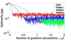
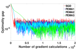
(a) Stochastic first-order projected (left) and proximal (right) methods.

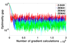
(b) Stochastic zeroth-order projected (left) and proximal (right) methods.

Figure 1: Convergence of different stochastic algorithms over 500 epochs for the robust phase retrieval problem.

We illustrate on the stochastic projected and proximal subgradient methods. We examine both cases with $d=10$ and $n=1000$ and record the result in Figure 1. In each set of experiments, we use $10$ equally spaced stepsize parameters $\alpha$ between $0.0001$ and $0.1$. The experiment is repeated ten times and the average accuracy and performance are depicted in Figure 1. It is clear from the panels in Figure 1 that Fema and Zema outperform Sgd and Z-Sgd algorithms in terms of the optimality gap $\Delta_{\psi}=\psi_{1/\bar{\rho},\widehat{V}_{-1}^{1/2}}(x_{0})-\psi^{*}$.

4.2 Neural networks

We present empirical results showcasing the important aspect of our framework–adaptiveness of learning rates. We test the performance of our models for training neural networks for classification tasks using the CIFAR10 and CIFAR100 datasets (60,000 $32\times 32$ images, 10 and 100 classes, respectively) [25]. For our experiment, we use Fema to train ResNets110 [22], which is very popular architecture, producing state-of-the-art results across many computer vision tasks. We adopt a standard data augmentation scheme (mirroring/shifting) that is widely used.

Method	$\alpha$	CIFAR-10	CIFAR-100
Sgd	1e-3	6.89 (6.11)	26.81 (25.31)
Fema1	1e-3	5.67 (5.41)	26.59 (25.08)
Fema2	1e-3	5.61(5.36)	25.83 (25.50)
Fema3	1e-3	5.51 (5.34)	25.02 (24.56)

Method	$\alpha$	CIFAR-100	CIFAR-100
Fema3	0.0001	6.51 (6.00)	26.33 (25.49)
	0.001	5.51 (5.34)	25.02 (24.56)
	0.005	5.73 (5.60)	25.68 (25.17)
	0.01	6.74 (6.12)	26.20 (25.24)

Table 2: ResNets110 test error (in %) on CIFAR-10 and CIFAR-100 datasets. All our experiments were run for 500 epochs with batch-size of 256. We report the mean error over the last 10 epochs and minimum error over all epochs (inside parenthesis) of the median error over five tries.

For our experiment, we use ELUs activation function [7] so that the loss is weakly convex.. As seen from Table 2, without any tuning, our default parameter setting achieves state-of-the-art results for this network. In particular, we see Fema3 consistently outperforming other algorithms, especially on the CIFAR-100 dataset. Further, as shown in Table 2 (right), our proposed parameterization $\alpha_{t}=\alpha=1e-3$ obtained the best accuracy.

5 Conclusion

In this paper, we examined first and zeroth order adaptive methods for nonconvex & nonsmooth optimization. We provided some mild sufficient conditions to ensure convergence of a class of adaptive algorithms, which include Adam and RMSprop as special cases. To the best of our knowledge, the convergence of adaptive algorithms for nonconvex and nonsmooth problems was unknown before. We also showed empirically on selected settings how adaptive algorithms can perform better than Sgd and its zeroth-order variants.

Appendix

Proof of Lemma 5

Proof.

Th proof is similar to that of [8, Theorem 3.1]. (i) $\Rightarrow$ (ii). Since $\psi$ is $(\rho,Q)$-weakly convex, it follows from Definition 4 that the function $\psi_{\rho,Q}(x):=\psi(x)+\frac{\rho}{2}\|Q^{1/2}x\|^{2}$ is convex. This implies that the subgradient $\partial\psi_{\rho,Q}(x)$ exists and can be computed as follows

$$\partial\psi_{\rho,Q}(x)\in\partial\psi(x)+\rho Qx.$$

Now, let $\varpi\in\partial\psi(x)$. By the convexity of $\psi_{\rho,Q}(x)$, we have

$$\psi_{\rho,Q}(y)\geq\psi_{\rho,Q}(x)+\langle\varpi+\rho Qx,y-x\rangle,\qquad\textnormal{for\, all\,}~{}~{}x,y\in\mathbb{R}^{d}.$$ (57)

By (57), we further have

$$\psi(y) \geq\psi(x)+\langle\varpi,y-x\rangle+\frac{\rho}{2}\|Q^{1/2}x\|^{2}-\frac{\rho}{2}\|Q^{1/2}y\|^{2}+\langle\rho Qx,y\rangle-\langle\rho Qx,x\rangle$$

$$=\psi(x)+\langle\varpi,y-x\rangle-\frac{\rho}{2}\|Q^{1/2}y\|^{2}-\frac{\rho}{2}\|Q^{1/2}x\|^{2}+\langle\rho Qx,y\rangle$$

$$=\psi(x)+\langle\varpi,y-x\rangle-\frac{\rho}{2}\|Q^{1/2}(y-x)\|^{2}.$$

(ii) $\Rightarrow$ (iii). For any $x,y\in\mathbb{R}^{d}$ with $\varpi\in\partial\psi(x)$ and $\omega\in\partial\psi(y)$, it follows from (3) that

$$\psi(y) \geq \psi(x)+\langle\varpi,y-x\rangle-\frac{\rho}{2}\|Q^{1/2}(y-x)\|^{2},$$

$$\psi(x) \geq \psi(y)+\langle\omega,x-y\rangle-\frac{\rho}{2}\|Q^{1/2}(x-y)\|^{2}.$$

Adding the above inequalities gives the desired result.
(iii) $\Rightarrow$ (i). It follows from (4) that

$$\langle\omega-\varpi,x-y\rangle\geq-\rho\|Q^{1/2}(y-x)\|^{2},$$

which yields

$$\langle\omega+\rho Qy-(\varpi+\rho Qx),y-x\rangle\geq 0.$$

As a result, the subdifferential of $\psi_{\rho,Q}(\cdot)$ is a globally monotone map. Applying [39, Theorem 12.17], we conclude that $\psi_{\rho,Q}(\cdot)$ is convex. ∎

Lemma 23.

[33, Lemma 1] Let $0\leq\beta_{1,t}\leq\beta_{1}$, $\{\beta_{i}\}_{i=1}^{3}\in[0,1)$ and $\tau=\beta_{1}/\sqrt{\beta_{2}}<1$. Then, for $m_{t}$ and $\widehat{V}_{t}$ generated by Algorithm 1, we have

$$\|\widehat{V}_{t}^{-1/4}m_{t}\|^{2}\leq\frac{\sum_{k=0}^{t}{\tau}^{t-k}\|{g_{k}}\|_{1}}{{(1-\beta_{1})\sqrt{(1-\beta_{2})(1-\beta_{3})}}}.$$

Lemma 24.

[33] Suppose Assumption B holds and $\|G(x,\xi)\|_{\infty}\leq G_{\infty}$ for all $x\in\mathcal{X}$ and $\xi\in\Omega$. Then, for $g_{t}$,$m_{t}$, and $\widehat{\upsilon}_{t}$ defined in Algorithm 1, we have $\|g_{t}\|_{\infty}\leq G_{\infty}$, $\|\widehat{\upsilon}_{t}^{1/2}\|_{\infty}\leq G_{\infty}$ and $\|m_{t}\|_{\infty}\leq G_{\infty}$.

Lemma 25.

[19, Lemma 6.3.a] Let $u$ be a $d$-dimensional random vector drawn uniformly from the sphere of a unit ball $B$ . Then,

$$\frac{1}{\mathcal{V}(d)}\int_{u\in B}\|u\|^{p}du=\frac{d}{d+p},\quad\textnormal{and}\quad\int_{u\in B}uu^{\top}du=\frac{\mathcal{V}(d)}{d}I.$$

Here, $\mathcal{V}(d)$ denotes the the volume of the unit ball in $\mathbb{R}^{d}$ and $I$ is the identity matrix in $\mathbb{R}^{d\times d}$.

References

• [1] H. Attouch. Variational convergence for functions and operators, volume 1. Pitman Advanced Publishing Program, 1984.
• [2] K. Balasubramanian and S. Ghadimi. Zeroth-order (non)-convex stochastic optimization via conditional gradient and gradient updates. In Advances in Neural Information Processing Systems, pages 3455–3464, 2018.
• [3] R. P. Brent. Algorithms for minimization without derivatives. Courier Corporation, 2013.
• [4] P.-Y. Chen, H. Zhang, Y. Sharma, J. Yi, and C.-J. Hsieh. Zoo: Zeroth order optimization based black-box attacks to deep neural networks without training substitute models. In Proceedings of the 10th ACM Workshop on Artificial Intelligence and Security, pages 15–26. ACM, 2017.
• [5] X. Chen, S. Liu, R. Sun, and M. Hong. On the convergence of a class of adam-type algorithms for non-convex optimization. arXiv preprint arXiv:1808.02941, 2018.
• [6] X. Chen, S. Liu, K. Xu, X. Li, X. Lin, M. Hong, and D. Cox. Zo-adamm: Zeroth-order adaptive momentum method for black-box optimization. In Advances in Neural Information Processing Systems, pages 7202–7213, 2019.
• [7] D.-A. Clevert, T. Unterthiner, and S. Hochreiter. Fast and accurate deep network learning by exponential linear units (elus). arXiv preprint arXiv:1511.07289, 2015.
• [8] A. Daniilidis and J. Malick. Filling the gap between lower-c1 and lower-c2 functions. Journal of Convex Analysis, 12(2):315–329, 2005.
• [9] D. Davis and D. Drusvyatskiy. Stochastic model-based minimization of weakly convex functions. SIAM Journal on Optimization, 29(1):207–239, 2019.
• [10] D. Davis and B. Grimmer. Proximally guided stochastic subgradient method for nonsmooth, nonconvex problems. SIAM Journal on Optimization, 29(3):1908–1930, 2019.
• [11] T. Dozat. Incorporating nesterov momentum into adam. 2016.
• [12] J. Duchi, E. Hazan, and Y. Singer. Adaptive subgradient methods for online learning and stochastic optimization. Journal of Machine Learning Research, 12(Jul):2121–2159, 2011.
• [13] J. C. Duchi, M. I. Jordan, M. J. Wainwright, and A. Wibisono. Optimal rates for zero-order convex optimization: The power of two function evaluations. IEEE Transactions on Information Theory, 61(5):2788–2806, 2015.
• [14] J. C. Duchi and F. Ruan. Stochastic methods for composite and weakly convex optimization problems. SIAM Journal on Optimization, 28(4):3229–3259, 2018.
• [15] M. Fickus, D. G. Mixon, A. A. Nelson, and Y. Wang. Phase retrieval from very few measurements. Linear Algebra and its Applications, 449:475–499, 2014.
• [16] J. R. Fienup. Phase retrieval algorithms: a comparison. Applied optics, 21(15):2758–2769, 1982.
• [17] J. R. Fienup. Reconstruction of a complex-valued object from the modulus of its fourier transform using a support constraint. JOSA A, 4(1):118–123, 1987.
• [18] M. C. Fu. Optimization for simulation: Theory vs. practice. INFORMS Journal on Computing, 14(3):192–215, 2002.
• [19] X. Gao, B. Jiang, and S. Zhang. On the information-adaptive variants of the admm: an iteration complexity perspective. Journal of Scientific Computing, 76(1):327–363, 2018.
• [20] S. Ghadimi and G. Lan. Stochastic first- and zeroth-order methods for nonconvx stochastic programming. SIAM Journal on Optimizatnoi, 23(4):2341–2368, 2013.
• [21] S. Ghadimi, G. Lan, and H. Zhang. Mini-batch stochastic approximation methods for nonconvex stochastic composite optimization. Mathematical Programming, 155(1-2):267–305, 2016.
• [22] K. He, X. Zhang, S. Ren, and J. Sun. Deep residual learning for image recognition. In 2016 IEEE Conference on Computer Vision and Pattern Recognition (CVPR), pages 770–778. IEEE, 2016.
• [23] R. A. Jacobs. Increased rates of convergence through learning rate adaptation. Neural networks, 1(4):295–307, 1988.
• [24] D. Kingma and J. Ba. Adam: A method for stochastic optimization. arXiv preprint arXiv:1412.6980, 2014.
• [25] A. Krizhevsky. Learning multiple layers of features from tiny images. Technical report, Citeseer, 2009.
• [26] J. D. Lee, Y. Sun, and M. A. Saunders. Proximal newton-type methods for minimizing composite functions. SIAM Journal on Optimization, 24(3):1420–1443, 2014.
• [27] X. Lian, H. Zhang, C.-J. Hsieh, Y. Huang, and J. Liu. A comprehensive linear speedup analysis for asynchronous stochastic parallel optimization from zeroth-order to first-order. In Advances in Neural Information Processing Systems, pages 3054–3062, 2016.
• [28] S. Liu, J. Chen, P.-Y. Chen, and A. O. Hero. Zeroth-order online alternating direction method of multipliers: Convergence analysis and applications. arXiv preprint arXiv:1710.07804, 2017.
• [29] S. Liu, P.-Y. Chen, X. Chen, and M. Hong. signsgd via zeroth-order oracle. 2018.
• [30] S. Liu, B. Kailkhura, P.-Y. Chen, P. Ting, S. Chang, and L. Amini. Zeroth-order stochastic variance reduction for nonconvex optimization. In Advances in Neural Information Processing Systems, pages 3727–3737, 2018.
• [31] L. Luo, Y. Xiong, Y. Liu, and X. Sun. Adaptive gradient methods with dynamic bound of learning rate. arXiv preprint arXiv:1902.09843, 2019.
• [32] P. Nazari, E. Khorram, and D. A. Tarzanagh. Adaptive online distributed optimization in dynamic environments. Optimization Methods and Software, pages 1–25, 2019.
• [33] P. Nazari, D. A. Tarzanagh, and G. Michailidis. Dadam: A consensus-based distributed adaptive gradient method for online optimization. arXiv preprint arXiv:1901.09109, 2019.
• [34] Y. Nesterov and V. Spokoiny. Random gradient-free minimization of convex functions. Foundations of Computational Mathematics, 17(2):527–566, 2017.
• [35] N. Parikh and S. Boyd. Proximal algorithms. Optimization, 1(3):127–239, 2014.
• [36] S. J. Reddi, S. Kale, and S. Kumar. On the convergence of adam and beyond. In International Conference on Learning Representations, 2018.
• [37] H. Robbins and S. Monro. A stochastic approximation method. In Herbert Robbins Selected Papers, pages 102–109. Springer, 1985.
• [38] R. T. Rockafellar. Convex analysis. Number 28. Princeton university press, 1970.
• [39] R. T. Rockafellar and R. J.-B. Wets. Variational analysis, volume 317. Springer Science & Business Media, 2009.
• [40] S. Shalev-Shwartz et al. Online learning and online convex optimization. Foundations and Trends® in Machine Learning, 4(2):107–194, 2012.
• [41] O. Shamir. An optimal algorithm for bandit and zero-order convex optimization with two-point feedback. Journal of Machine Learning Research, 18(52):1–11, 2017.
• [42] Y. Shechtman, Y. C. Eldar, O. Cohen, H. N. Chapman, J. Miao, and M. Segev. Phase retrieval with application to optical imaging: a contemporary overview. IEEE signal processing magazine, 32(3):87–109, 2015.
• [43] T. Tieleman and G. Hinton. Divide the gradient by a running average of its recent magnitude. coursera: Neural networks for machine learning. Technical report, Technical Report. Available online: https://zh. coursera. org/learn/neuralnetworks/lecture/YQHki/rmsprop-divide-the-gradient-by-a-running-average-of-its-recent-magnitude (accessed on 21 April 2017).
• [44] J.-P. Vial. Strong and weak convexity of sets and functions. Mathematics of Operations Research, 8(2):231–259, 1983.
• [45] R. Ward, X. Wu, and L. Bottou. Adagrad stepsizes: Sharp convergence over nonconvex landscapes, from any initialization. arXiv preprint arXiv:1806.01811, 2018.
• [46] M. Zaheer, S. Reddi, D. Sachan, S. Kale, and S. Kumar. Adaptive methods for nonconvex optimization. In Advances in Neural Information Processing Systems, pages 9793–9803, 2018.
• [47] M. D. Zeiler. Adadelta: an adaptive learning rate method. arXiv preprint arXiv:1212.5701, 2012.
• [48] S. Zhang and N. He. On the convergence rate of stochastic mirror descent for nonsmooth nonconvex optimization. arXiv preprint arXiv:1806.04781, 2018.
• [49] D. Zhou, Y. Tang, Z. Yang, Y. Cao, and Q. Gu. On the convergence of adaptive gradient methods for nonconvex optimization. arXiv preprint arXiv:1808.05671, 2018.