Assertion Detection in Multi-Label Clinical Text using Scope Localization

Abstract

Multi-label sentences (text) in the clinical domain result from the rich description of scenarios during patient care. The state-of-the-art methods for assertion detection mostly address this task in the setting of a single assertion label per sentence (text). In addition, few rules based and deep learning methods perform negation/assertion scope detection on single-label text. It is a significant challenge extending these methods to address multi-label sentences without diminishing performance. Therefore, we developed a convolutional neural network (CNN) architecture to localize multiple labels and their scopes in a single stage end-to-end fashion, and demonstrate that our model performs atleast 12% better than the state-of-the-art on multi-label clinical text.

1 Introduction

In recent years, advanced natural language processing (NLP) techniques have been applied to electronic health record (EHR) documents to extract useful information. Accessibility to large scale EHR data is very crucial to using such deep learning methods - yet data scarcity persists for most tasks in the healthcare domain.

Assertion detection involves classifying clinical text obtained from the EHR and other hospital information systems (e.g. Radiology Information System/RIS), to determine if a medical concept (entity) is present, absent, conditional, hypothetical, possibility or AWSE (associated with someone else). These classes were used in Chen (2019). A few examples of each class from our dataset are shown in Table. 1.

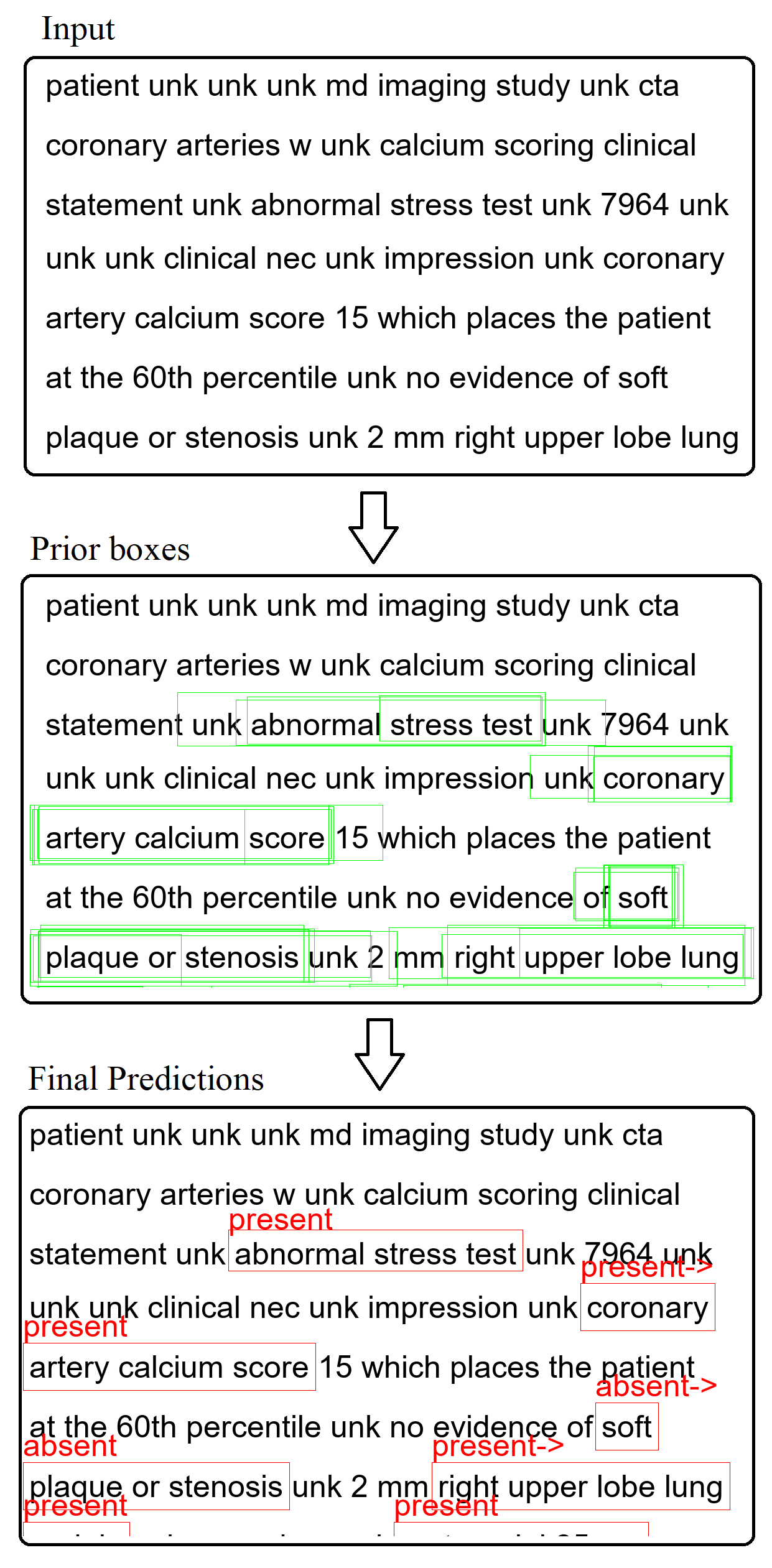
Figure 1: From the Input, the model will predict confidence scores for all the prior boxes at each token. Prior boxes with confidence threshold greater than $\gamma$ are shown in green. After non-max suppression, the final predictions are shown in red.

Past works with the i2b2 dataset mostly focused on the present and absent classes with comparatively less work on the more ambiguous classes. Majority of the existing methods either classify the given text only, or use the class further to detect it’s scope in a two stage process. This works well for datasets like i2b2 (Uzuner et al., 2011) in which there exists only one label per example. However, single label per sentence is not a common phenomenon in clinical reports, especially when patients have frequent physician visits or long periods of hospitalization. To address the aforementioned problem, our work highlights the following contributions:

• We explored assertion detection in multi-label sentences from radiology (cardiac computerized tomography (CT)) reports.

• We cast the assertion detection task as a scope localization problem, thereby solving classification and scope detection in a single stage end-to-end fashion.

• We leveraged concepts from object localization Redmon et al. (2015) in computer vision and developed a CNN to detect bounding boxes around class scopes.

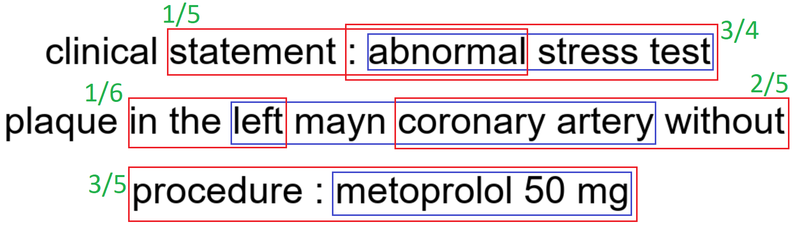
Figure 2: The blue boxes are ground-truths. The IoU of each of the red boxes with the blue boxes are shown in green.

2 Related Work

Rule based models like NegExChapman et al. (2011), NegBio Peng et al. (2017) and Gkotsis et al. (2016) were initially used for assertion and negation detection. These approaches typically implement rules and regular expressions to detect cues for classification. NegBio Peng et al. (2017) uses a universal dependency graph to detect the scope of identified class. A constituency parsed tree is used by Gkotsis et al. (2016) to prune out words outside the scope of the detected class. NegEx Chapman et al. (2011) later demonstrated good performance when adapted to many other languages like German, Spanish and French Cotik et al. (2015); Stricker et al. (2015); Costumero et al. (2014); Afzal et al. (2014). A few approaches developed syntactic techniques by augmenting dependency parsed trees to rule based systems Mehrabi et al. (2015); Sohn et al. (2012); Cotik et al. (2016). Mackinlay et al. (2012) constructed hand-engineered features using English Resource Grammar to identify negation and hypothetical classes for a BIONLP 2009 task.

Class	Examples
Present	Metoprolol 50 mg po was administered prior to the scan to decrease heart rate
Absent	No Chest pain, No Coronary artery Aneurysm, No Aneurysm or wall thickening
Conditional	Myocardial perfusion imaging, if not already performed, might improve specificity in this regard if clinically warranted
Hypothetical	Coronary plaque burden and focal Lesion characterization (if present) were assessed by visual estimate.
Possibility	This was incompletely imaged but suggests a diaphragmatic arteriovenous malformation
AWSE	High risk is $>$ or = 10 packs/year or positive family history of lung cancer in first degree relative

Table 1: Examples of each class from our dataset. From each sentence (or phrase) shown, the text in bold is identified as the corresponding class.

The annotated entities and assertion /labels in the 2010 i2b2/VA challenge (Uzuner et al., 2011) can be regarded as a benchmark for the assertion detection task for clinical text. Kernel methods using SVM (de Bruijn et al., 2011) and Bag-of-Words (Shivade et al., 2015) were proposed for the shared task. Cheng et al. (2017) used a CRF for classification of cues and scope detection. Though these methods have performed better than rule based methods, they fail to generalize well to unseen examples while training.

More recently, with the advent of deep learning achieving state-of-the-art performance in various NLP tasks, an LSTM encoder-decoder architecture (Sutskever et al., 2014) (Hochreiter and Schmidhuber, 1997) can be trained for assertion detection with reasonable success. Attention based models using LSTMs (Fancellu et al., 2016) and GRUs (Rumeng et al., 2017) were explored. Limited amounts of labeled (and unlabeled) clinical text make training deep neural networks a challenging task. Bhatia et al. (2018) explored a multi-task learning setting by combining a Named Entity Recognition (NER) classification branch to the assertion detection output. All of these methods either identify only the class or use it as a cue to prune the scope of the class from the text. As mentioned above, our work proposes an end-to-end single stage approach to assertion and negation scope detection. A schematic of our approach is shown in Fig.1.

3 Proposed Model

We formulated the assertion and negation problem as follows: Let $R=\{r_{1},r_{2},...,r_{T}\}$ be a sentence in clinical report consisting of $T$ words $r_{i}$. We need to identify the $L$ assertion classes and corresponding scope in the report defined by the set $S=\{(c_{1},x_{1},y_{1}),(c_{2},x_{2},y_{2}),...,(c_{L},x_{L},y_{L})\}$ where, class $c_{i}$ scopes between $x_{i}\in[1,T]$ and $y_{i}\in[1,T]$. We put forward this problem as finding bounding boxes over the text that scope a particular class. If $A$ is the maximum scope of a class present in the input, we can place prior boxes of lengths $\{1,2,..,A\}$ at each word $r_{i}$ and predict the probability of a particular box containing a class.

3.1 Intersection Over Union

Let $B_{1},B_{2}$ be two bounding boxes over text scopes $T_{1},T_{2}$ where, $T_{i}$ is a set of words. We then define the IoU (Intersection over Union) of these two bounding boxes as follows:

$$IoU(B_{1},B_{2})=\frac{|T_{1}\cap T_{2}|}{|T_{1}\cup T_{2}|}$$ (1)

Where $|S|$ is the cardinal of a set $S$. A few examples if IoUs are shown in Fig.2.

3.2 Network Design

First, we embed the input sequence in a distributional word vector space as $W=\{e_{1},e_{2},...,e_{T}\}$ where, $e_{i}\in\mathbb{R}^{D}$ is a column vector in an embedding matrix $E\in R^{T\times D}$. This is the input to our CNN. Each layer in the CNN is a 1D-convolutional layer followed by a non-linearity. Stacking many layers on top of the other increases the receptive field of the network. To cover the largest prior box of length $A$, we need the receptive field of the last layer to be at least $A$.

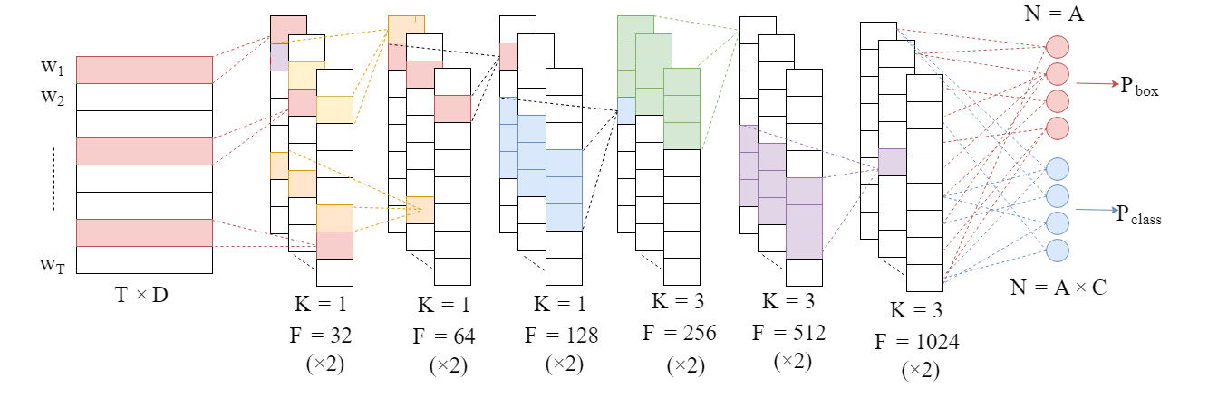
Figure 3: CNN Architecture: The input sequence is first passed through a pretrained embedding layer. $\times 2$ denotes two layers of same kernel size and no. of filters. First 6 layers use a kernels of size 1 and last 6 layers use kernels of size 3. The no. of filters double every two layers. Here, K, F and N are kernel size, filter size and number of units respectively. The feature map of the last convolutional layer is projected using two fully-connected layers of units $A$ and $A\times C$ respectively. The resulting box confidence and class confidence probabilities are fed to the MSE and cross-entropy loss functions respectively.

Our architecture is shown in Fig.3. First we use 6 layers of $1\times 1$ convolutions followed by 6 layers of $3\times 1$ convolutions. We use a stride of 1 and pad the feature maps wherever necessary to maintain constant feature map size of $T$ throughout the network. We also use ReLU non-lineartiy after each convolutional layer. The output of the last convolutional layer is then passed through 2 branches of fully-connected layers to produce box confidence scores $p_{box}\in\mathbb{R}^{T\times A}$ and class confidence probabilities $p_{class}\in\mathbb{R}^{T\times A\times C}$ respectively. Where, $A$ is the number of prior boxes and $C$ is the number of classes. It is important to note the receptive field of the last layer is 24.

3.3 Objective Function

Box Confidence Loss: We expect the box confidence branch to predict the IoU of each prior box with the nearest ground truth box. The simplest way to do this is by minimizing the Mean Square Error (MSE) between predicted and ground-truth IoU.

$$L_{box}=\frac{1}{T\times A}\sum_{t=1}^{T}\sum_{a=1}^{A}\lVert p_{box}(t,a)-iou\rVert_{2}^{2}$$ (2)

Non-max Suppression Once we have the box confidence scores of $T*A$ prior boxes, we sort them in the decreasing order of their confidence scores and discard the ones lower than a confidence threshold $\gamma$. In the remaining overlapping boxes, we vote for the prior box with high confidence score. The detailed algorithm is shown in Algorithm 1.

Class Confidence Loss: The class confidence branch is expected to predict $P(class|box)$, the probability of a class given that a prior box has an assertion scope. We first apply softmax on the class confidence score and use cross-entropy loss to maximize the probability of the ground-truth class. Given the class imbalance in the dataset we used, a weighted loss per class was implemented.

$$L_{class}=\frac{1}{T\times A}\sum_{t=1}^{T}\sum_{a=1}^{A}\mathds{1}_{box}^{a}\sum_{c=1}^{C}-w_{c}\mathds{1}_{c}\log(p_{class}(c))$$ (3)

Where, $\mathds{1}_{box}^{a}$ is an indicator variable denoting the presence of a class in prior box-$a$ and $w_{c}$ is the weight of class-$c$ which is equal to the fraction of examples in a batch that belong to class-$c$.

We optimize the cummulative loss $L=L_{box}+L_{class}$ using Adam optimizer.

Result: Final non-overlapping boxes

$indices=ArgSort(scores)$ ;

$boxes=[]$ ;

$i=0$ ;

while $i\leq T*A$ do

       if $scores(i)\leq\gamma$ then

             break;

            

      else

             $maxIoU\leftarrow max(IoU(priors[i],boxes))$ ;

             if maxIoU == 0 then

                   $boxes\leftarrow[boxes,priors[i]]$ ;

                  

             end if

            

       end if

      $i\leftarrow i+1$ ;

      

end while

Algorithm 1 NonMaxSup(scores, priors)

4 Datasets and Experiments

We evaluated our model on datasets from two hospital sites (Dataset-I and Dataset-II); both have reports with multi-label sentences. First we will elaborate on the data collection and annotation process. Next, we will present some statistics on the datasets and, finally, highlight the performance of our model. Dataset-I and II comprise 151 and 460 cardiac CT reports respectively. All reports were anonymized at the hospital site before we accessed the data. The datasets were annotated by 8 engineers with an average of 217 hours of training in labeling healthcare data.

The annotations were done using BRAT tool (Stenetorp et al., 2012). Rules for annotation were generated after consulting with the Radiologist supervising the annotators. Other Radiologists were consulted to annotate any mentions that were previously unseen or ambiguous and also for the final review. Statistics of the data such as No. of classes per report, No. of tokens in a report and length of class scopes are shown in Tables.5-5.

Class	Dataset-I			Dataset-II
	Train	Val	Test	Train	Val	Test
Present	3711	511	524	17407	2215	2452
Absent	596	73	73	6136	708	805
Conditional	169	31	19	393	44	49
Hypothetical	147	22	18	69	10	5
Possibility	62	5	11	219	37	25
AWSE	15	3	2	21	4	2

Table 2: Distribution of Assertion classes in the data.

Split	Dataset-I			Dataset-II
	Max	Min	Mean	Max	Min	Mean
train	661	19	440	1028	82	610
val	642	289	452	911	82	630
test	560	228	432	968	336	642

Table 3: Number of tokens per report in the data.

Class	Dataset-I			Dataset-II
	Train	Val	Test	Train	Val	Test
1	$3.36\pm 2.7$	$3.23\pm 2.59$	$3.39\pm 2.95$	$3.48\pm 2.15$	$3.38\pm 2.06$	$3.48\pm 2.16$
2	$2.79\pm 1.36$	$2.68\pm 1.25$	$2.68\pm 1.07$	$3.15\pm 2.26$	$3.10\pm 2.18$	$3.09\pm 2.13$
3	$2.85\pm 1.04$	$2.87\pm 0.87$	$2.68\pm 0.65$	$3.24\pm 2.92$	$3.20\pm 1.95$	$2.60\pm 1.74$
4	$5.05\pm 2.44$	$4.5\pm 2.44$	$5.0\pm 2.43$	$2.19\pm 1.21$	$2.60\pm 0.92$	$2.84\pm 2.47$
5	$3.14\pm 3.69$	$1.67\pm 0.47$	$3.27\pm 2.41$	$2.96\pm 2.83$	$2.40\pm 1.82$	$3.27\pm 2.41$
6	$2.47\pm 0.72$	$1.67\pm 0.47$	$5.5\pm 2.5$	$1.71\pm 1.35$	$2.00\pm 1.73$	$1.0\pm 0.0$

Table 4: Scope lengths of each class per train, validation (val) and test splits. Following are the classes corresponding to the IDs 1: Present, 2: Absent, 3: Conditional, 4: Hypothetical, 5: Possibility, 6: AWSE and macro $F_{1}$ score is the average over all classes. Lengths are written in the format $\mu\pm\sigma$.

Class	Model
	Baseline		Scope Localization model
	Dataset-I	Dataset-II	Dataset-I	Dataset-II
Present	0.97	0.92	0.90	0.84
Absent	0.27	0.34	0.84	0.93
Conditional	0.39	0.45	0.74	0.65
Hypothetical	0.76	0.69	0.87	0.75
Possibility	0.0	0.07	0.0	0.13
AWSE	0.42	0.39	0.60	0.0
None	0.81	0.89	0.96	0.95
Macro	0.52	0.53	0.70	0.61

Table 5: The performance of both baseline and our CNN model on Dataset-I and Dataset-II in terms of $F_{1}$ score. macro $F_{1}$ score is the average over all classes.

4.1 Baseline Model

(Bhatia et al., 2018; Chen, 2019; Rumeng et al., 2017). Chen (2019) used a bidirectional attentive encoder on the sentence input to obtain a context vector which is subsequently passed to the softmax and output classification layers. Bhatia et al. (2018) extended this network by adding a shared decoder to predict both assertion class and named entity tag in a multi-task learning framework. However, the input to these seq2seq models is a sentence and the output prediction is a single class. Therefore, the models may not be easily extended to a multi-label dataset without compromising performance. To validate our assumption, we extend the bidirectional encoder and attentive decoder model based on LSTM to our multi-label data by changing the input format. In other words, instead of predicting one class for the entire input sequence, we predict a class for each token so that the scope of a class can also be localized. Two sample sentences (with class labels) are shown in Table.6.

Report-1	MetoprololP 50P mgP poN wasN administeredN priorN toN theN scanN toN decreaseC heartC rateC
Report-2	MyocardialH perfusionH imagingH ,N ifN notN alreadyN performedN ,N mightH improveH specificityH inN thisN regardN ifN clinicallyN warrantedN .N

Table 6: Two sample sentences with the label format for the baseline seq2seq model. P, C, H, N denote present, conditional, hypothetical and none classes respectively.

4.2 Training and Hyperparameters

Since the datasets have unbalanced classes, we have used stratified sampling Sechidis et al. (2011); Szymański and Kajdanowicz (2017) to represent the classes in the same ratio in train, validation and test sets. To further mitigate the effect of unbalanced classes in each batch of training data, we weighted the cross entropy loss with the inverse of the number of examples for each class. The pre-trained BioWord2Vec (Zhang et al., 2019) is used in the embedding layer with frozen weights. We used Adam Optimizer with the default learning rate of 0.001 for 400 epochs. Shuffling after each epoch results in different distribution of classes per batch of iteration. This leads to unstable training and therefore takes more epochs for convergence. We have set the number of prior boxes to be 24, little more than the maximum length of a class scope in the training set. Fig-4 shows the performance of the model on validation set with different values of IoU threshold ($\gamma$), the maximum being $\gamma=0.7$. Experiments with more layers and higher kernel sizes didn’t improve the performance. This is because the receptive field has to be large enough to span the longest scope in the input i.e 20.

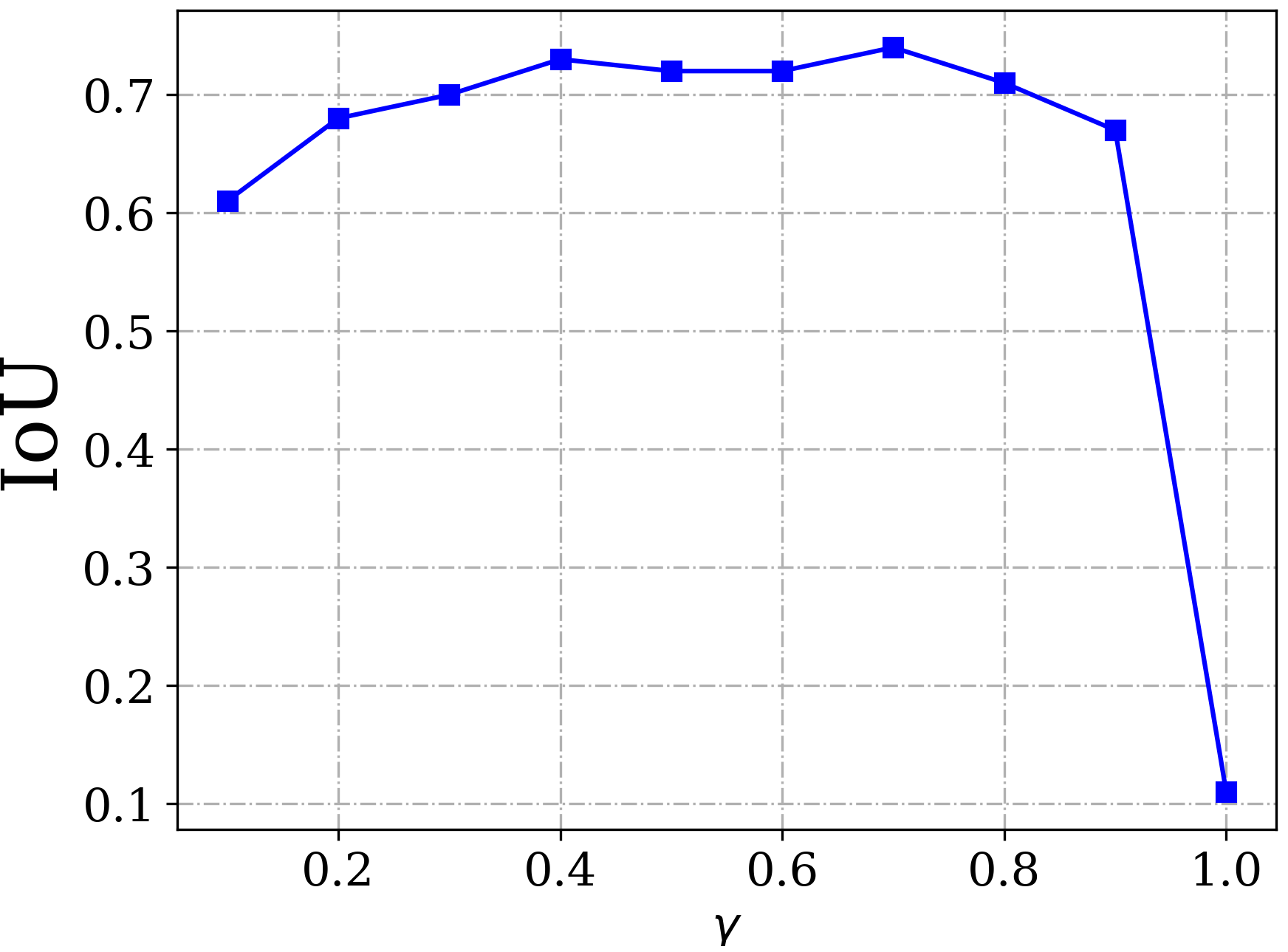
Figure 4: F1 score with different values of IOU threshold evaluated on the validation set

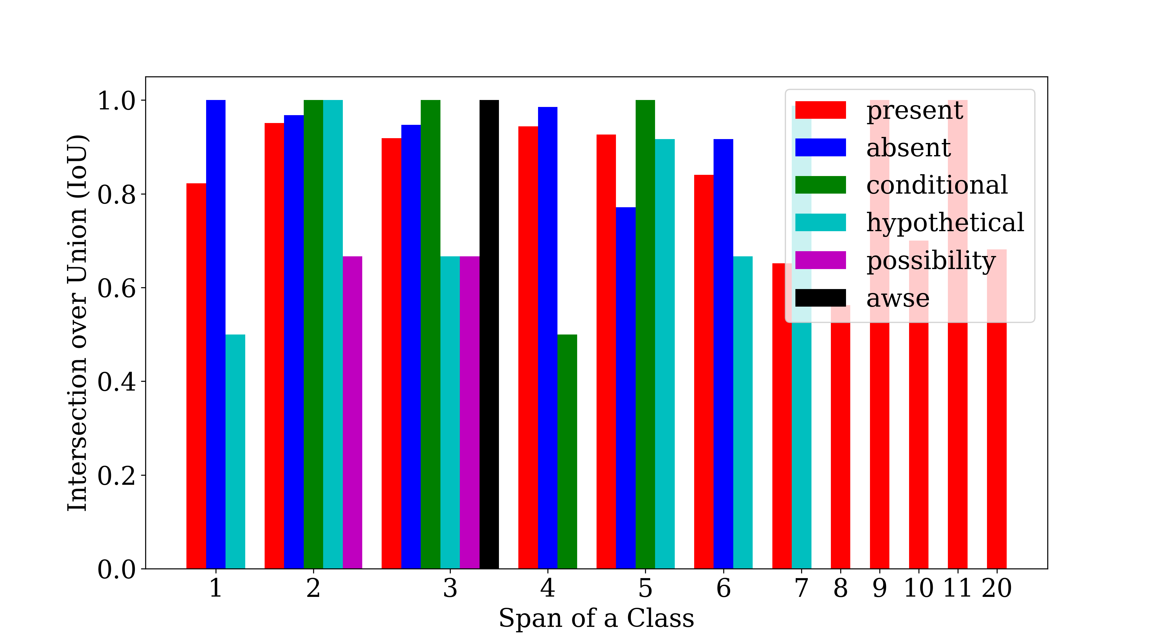
Figure 5: This figure shows the IoU (Intersection over Union) between the predictions and ground-truths on test set for different scope lengths.

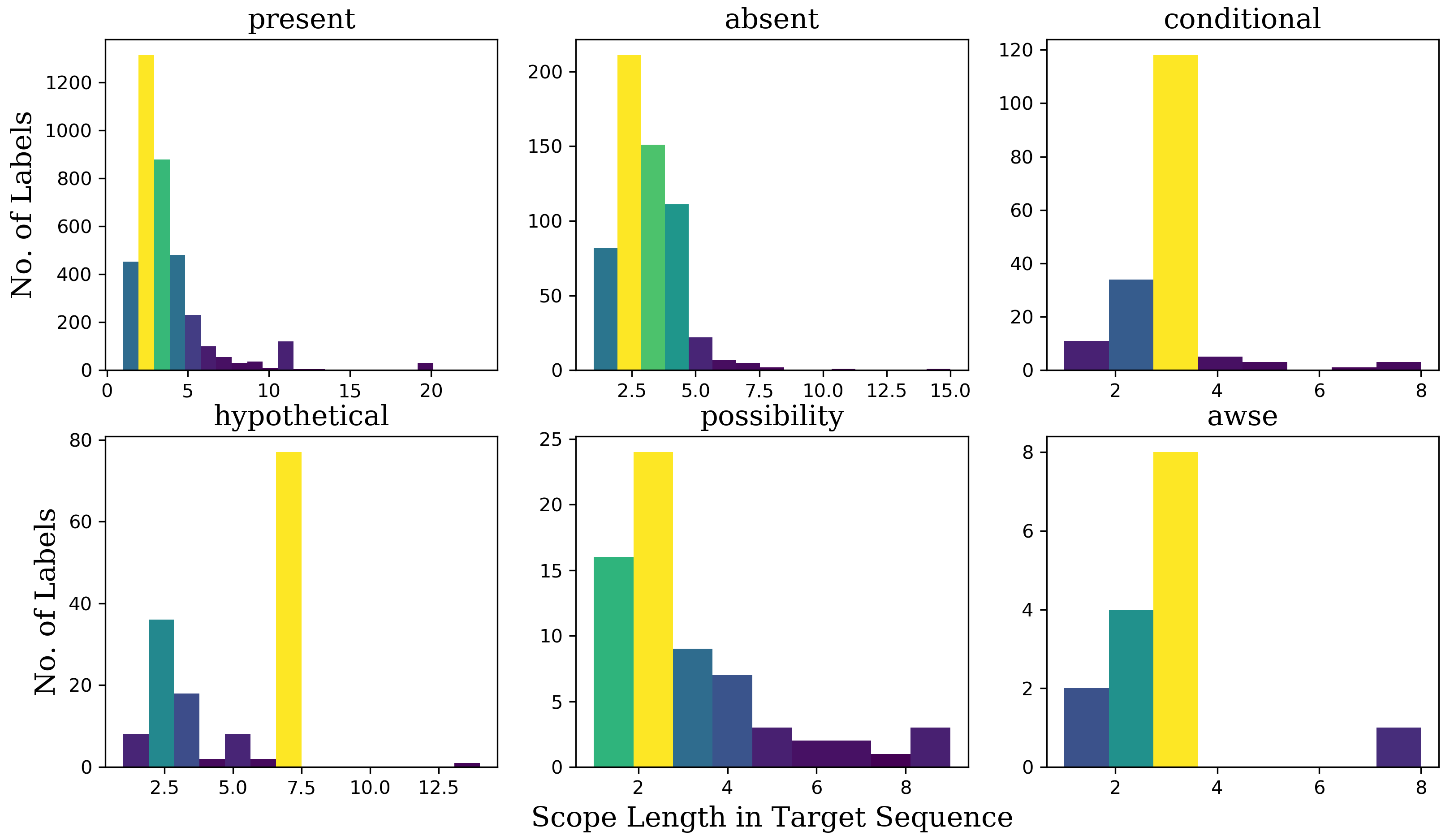
Figure 6: This figure shows histograms of scope lengths per each class in the training set.

Figure 7: A sample output of the model on a report from Dataset-I. The ground-truths are shown in blue. The green boxes are prior boxes each having a box-confidence score. After non-max suppression of these prior boxes, the final predictions are shown in blue. $"->"$ is used to indicate that the box is extended to next line. ”unk” represents the unknown token, it is used to represent the words that are not found in the vocabulary.

4.3 Results

Table.5 shows the performance of the baseline and our CNN-based scope localization models on Datasets-I,II per each class. For a fair comparison with the baseline, the box predictions from our model are converted to a sequence of labels per token. On first impressions, the performance seem to be affected by the quantity of data available for training with the best performance on present class and least performance on AWSE class. After further analysis, it appears that the scope lengths found in the training set is also a crucial factor. Fig.6 shows a histogram of scope lengths available in the training set for each class. The performance on the test set for different scope lengths is shown in Fig.5. As shown, model performance for the present class declines with scope lengths 7, 10, and 20, which reflect sparsity of this class for these scopes in the training set. In contrast, the model performs well on the hypothetical class with scope length 7, reflective of the better distribution of this class for this scope relative to other scopes.

5 Conclusion

In this work, we have explored a novel approach of scope localization and classification with a single end-to-end CNN model. We demonstrated good performance and thereby make a case for using multi-label clinical text that is often found in real world. For future work, we would like to explore the usage of inception layers; different sets of kernel sizes in each layer. The output layer will then have varying receptive fields i.e scope lengths in our problem. This increases the generalization of the model to scope lengths that are unseen in the training data.

References

- Afzal et al. (2014) Zubair Afzal, Ewoud Pons, Ning Kang, Miriam C. J. M. Sturkenboom, Martijn J. Schuemie, and Jan A. Kors. 2014. Contextd: an algorithm to identify contextual properties of medical terms in a dutch clinical corpus. In BMC Bioinformatics.
- Bhatia et al. (2018) Parminder Bhatia, Busra Celikkaya, and Mohammed Khalilia. 2018. End-to-end joint entity extraction and negation detection for clinical text. CoRR, abs/1812.05270.
- de Bruijn et al. (2011) Berry de Bruijn, Colin Cherry, Svetlana Kiritchenko, Joel D. Martin, and Xiao-Dan Zhu. 2011. Machine-learned solutions for three stages of clinical information extraction: the state of the art at i2b2 2010. In JAMIA.
- Chapman et al. (2011) Wendy W. Chapman, Will Bridewell, Paul Hanbury, Gregory F. Cooper, and Bruce G. Buchanan. 2011. A simple algorithm for identifying negated findings and diseases in discharge summaries. Journal of the American Medical Informatics Association, 18(5):552 – 556.
- Chen (2019) Long Chen. 2019. Attention-based deep learning system for negation and assertion detection in clinical notes. International Journal of Artificial Intelligence and Applications, 10:1–9.
- Cheng et al. (2017) Katherine Cheng, Timothy Baldwin, and Karin Verspoor. 2017. Automatic negation and speculation detection in veterinary clinical text. In Proceedings of the Australasian Language Technology Association Workshop 2017, pages 70–78, Brisbane, Australia.
- Costumero et al. (2014) Roberto Costumero, Federico Lopez, Consuelo Gonzalo-Martín, Marta Millan, and Ernestina Menasalvas. 2014. An approach to detect negation on medical documents in spanish. In Brain Informatics and Health, pages 366–375. Springer International Publishing.
- Cotik et al. (2015) Viviana Cotik, Dar´ıo Filippo, and Jos´e Casta˜no. 2015. An approach for automatic classification of radiology reports in spanish. In In Proceedings of 15th MEDINFO, pages 634–638.
- Cotik et al. (2016) Viviana Cotik, Vanesa Stricker, Jorge Vivaldi, and Horacio Rodriguez. 2016. Syntactic methods for negation detection in radiology reports in Spanish. In Proceedings of the 15th Workshop on Biomedical Natural Language Processing, pages 156–165, Berlin, Germany. Association for Computational Linguistics.
- Fancellu et al. (2016) Federico Fancellu, Adam Lopez, and Bonnie Webber. 2016. Neural networks for negation scope detection. In Proceedings of the 54th Annual Meeting of the Association for Computational Linguistics (Volume 1: Long Papers), pages 495–504, Berlin, Germany. Association for Computational Linguistics.
- Gkotsis et al. (2016) George Gkotsis, Sumithra Velupillai, Anika Oellrich, Harry Dean, Maria Liakata, and Rina Dutta. 2016. Don’t let notes be misunderstood: A negation detection method for assessing risk of suicide in mental health records. In Proceedings of the Third Workshop on Computational Linguistics and Clinical Psychology, pages 95–105, San Diego, CA, USA. Association for Computational Linguistics.
- Hochreiter and Schmidhuber (1997) Sepp Hochreiter and Jürgen Schmidhuber. 1997. Long short-term memory. Neural Comput., 9(8):1735–1780.
- Mackinlay et al. (2012) Andrew Mackinlay, David Martinez, and Timothy Baldwin. 2012. Detecting modification of biomedical events using a deep parsing approach. BMC medical informatics and decision making, 12 Suppl 1:S4.
- Mehrabi et al. (2015) Saeed Mehrabi, Anand Krishnan, Sunghwan Sohn, Alexandra M. Roch, Heidi Schmidt, Joe Kesterson, Chris Beesley, Paul R. Dexter, C. Max Schmidt, Hongfang Liu, and Mathew J. Palakal. 2015. Deepen: A negation detection system for clinical text incorporating dependency relation into negex. Journal of biomedical informatics, 54:213–9.
- Peng et al. (2017) Yifan Peng, Xiaosong Wang, Le Lu, Mohammadhadi Bagheri, Ronald M. Summers, and Zhiyong Lu. 2017. Negbio: a high-performance tool for negation and uncertainty detection in radiology reports. CoRR, abs/1712.05898.
- Redmon et al. (2015) Joseph Redmon, Santosh Kumar Divvala, Ross B. Girshick, and Ali Farhadi. 2015. You only look once: Unified, real-time object detection. CoRR, abs/1506.02640.
- Rumeng et al. (2017) Li Rumeng, N JagannathaAbhyuday, and Yu H. Hong. 2017. A hybrid neural network model for joint prediction of presence and period assertions of medical events in clinical notes. AMIA … Annual Symposium proceedings. AMIA Symposium, 2017:1149–1158.
- Sechidis et al. (2011) Konstantinos Sechidis, Grigorios Tsoumakas, and Ioannis Vlahavas. 2011. On the stratification of multi-label data. In Proceedings of the 2011 European Conference on Machine Learning and Knowledge Discovery in Databases - Volume Part III, ECML PKDD’11, pages 145–158, Berlin, Heidelberg. Springer-Verlag.
- Shivade et al. (2015) Chaitanya Shivade, Marie-Catherine de Marneffe, Eric Fosler-Lussier, and Albert M. Lai. 2015. Extending NegEx with kernel methods for negation detection in clinical text. In Proceedings of the Second Workshop on Extra-Propositional Aspects of Meaning in Computational Semantics (ExProM 2015), pages 41–46, Denver, Colorado. Association for Computational Linguistics.
- Sohn et al. (2012) Sunghwan Sohn, Stephen Wu, and Christopher G. Chute. 2012. Dependency parser-based negation detection in clinical narratives. In AMIA Joint Summits on Translational Science proceedings. AMIA Joint Summits on Translational Science.
- Stenetorp et al. (2012) Pontus Stenetorp, Sampo Pyysalo, Goran Topić, Tomoko Ohta, Sophia Ananiadou, and Jun’ichi Tsujii. 2012. Brat: A web-based tool for nlp-assisted text annotation. In Proceedings of the Demonstrations at the 13th Conference of the European Chapter of the Association for Computational Linguistics, EACL ’12, pages 102–107, Stroudsburg, PA, USA. Association for Computational Linguistics.
- Stricker et al. (2015) Vanesa Stricker, Ignacio Iacobacci, and V. Cotik. 2015. Negated findings detection in radiology reports in spanish: an adaptation of negex to spanish. In In IJCAI - Workshop on Replicability and Reproducibility in Natural Language Processing: adaptative methods, resources and software, Buenos Aires, Argentina.
- Sutskever et al. (2014) Ilya Sutskever, Oriol Vinyals, and Quoc V. Le. 2014. Sequence to sequence learning with neural networks. CoRR, abs/1409.3215.
- Szymański and Kajdanowicz (2017) P. Szymański and T. Kajdanowicz. 2017. A scikit-based Python environment for performing multi-label classification. ArXiv e-prints.
- Uzuner et al. (2011) Ozlem Uzuner, Brett R. South, Shuying Shen, and Scott L. DuVall. 2011. 2010 i2b2/va challenge on concepts, assertions, and relations in clinical text. Journal of the American Medical Informatics Association, 18(5):552 – 556.
- Zhang et al. (2019) Yijia Zhang, Qingyu Chen, Zhihao Yang, Hongfei Lin, and Zhiyong Lu. 2019. Biowordvec, improving biomedical word embeddings with subword information and mesh. In Scientific Data.