Multi-Period Liability Clearing
via Convex Optimal Control

Abstract

We consider the problem of determining a sequence of payments among a set of entities that clear (if possible) the liabilities among them. We formulate this as an optimal control problem, which is convex when the objective function is, and therefore readily solved. For this optimal control problem, we give a number of useful and interesting convex costs and constraints that can be combined in any way for different applications. We describe a number of extensions, for example to handle unknown changes in cash and liabilities, to allow bailouts, to find the minimum time to clear the liabilities, or to minimize the number of non-cleared liabilities, when fully clearing the liabilities is impossible.

1 Introduction

Large, complex networks of liabilities are the foundation of modern financial systems. According to the FDIC, there were on the order of five thousand FDIC-insured banks in the United States at the end of 2019 [Fed19]. Each of these banks owe each other money as a result of bank transfers, loans, and securities issued. Inter-bank settlement is handled today by simple payment systems like Fedwire and CHIPS [BH12, §2.4]. Another example of complex liability networks are derivatives exchanges and brokerages, where there are liabilities between clients in the form of derivatives contracts or borrowed shares. A goal shared by all of the entities in these systems is to clear or remove liabilities, which reduces risk and complexity. Each system has its own goals and constraints in its mission to clear liabilities, which must be accounted for.

We consider the general problem of liability clearing, which is to determine a sequence of payments between a set of financial entities to clear (if possible) the liabilities among them over a finite time horizon. We first observe that the dynamics in liability clearing are linear, and describe methods that can be used to remove cycles of liability before any payments are made. We then formulate liability clearing as an optimal control problem with convex objectives and constraints, where the system’s state is the cash held by each entity and the liabilities between each entity, and the input to the system is the payments made by each entity to other entities. This formulation has several benefits. First, we can naturally incorporate the goals and constraints in liability clearing in the stage cost function of our optimal control problem. Second, we can efficiently (globally) solve the problem since it is convex. Third, domain specific languages for convex optimization make it easy to prototype new liability clearing mechanisms.

We also extend our formulation to the case where there are exogenous unknown inputs to the dynamics, which represent uncertain future liabilities or cash flows. We propose a solution method based on model predictive control, or shrinking horizon control, which, at each time step, predicts the future unknown inputs, plans a sequences of payments, and then uses just the first of those payments for the next time period. We then illustrate our method on several simulated numerical examples, comparing to a simple pro-rata payment baseline. At the end of the paper, we discuss extensions and variations of our problem, e.g., allowing bailouts, finding the minimum time to clear a set of liabilities, non-time-separable costs, infinite time liability control, and how to minimize the number of non-cleared liabilities.

Outline.

In §2 we discuss related work as well as its relation to our paper. In §3 we set out our notation, and describe the dynamics equations and constraints. In §4 we formulate liability clearing as a convex optimal control problem, and describe a number of useful and interesting convex costs and constraints. In §5 we extend the optimal control formulation to the case where the dynamics are subject to additional uncontrollable exogenous terms, and propose a standard method called model predictive control for this problem. In §6 we illustrate the methods described in this paper by applying them to several numerical examples. In §7 we conclude with a number of extensions and variations on our formulation.

2 Related work

The liability clearing problem was originally proposed by Eisenberg and Noe in 2001 [EN01]. Their formulation involves determining a single set of payments to be made between the entities, in contrast to ours, which assumes a sequence of payments are made. Their formulation assumes that these payments can be financed immediately by payments received, whereas we make the realistic financing constraint that entities cannot pay other entities more than the cash they have on hand. (This means that it may take multiple steps to clear liabilities.) In this way, our formulation can be viewed as a supply chain with cash as the commodity [BV18, §9.5], while their formulation can be viewed as a network flow problem [HR55], where cash can travel multiple steps through the network at once.

They also make the assumption that all liabilities have equal priority [EN01, §2.2], i.e., each entity makes payments proportional to its liabilities to the other entities (we call this a pro-rata constraint; see §4.2). This means that instead of choosing a matrix of payments between all the entities, they only need to choose a vector of payments made by the entities; the payments are then distributed according to the proportion of liability (they call this vector the clearing vector). Our formulation can include the constraint that payments are made in proportion to liability, but we observe that enforcing this constraint at each step is not the most efficient strategy for clearing liabilities (see §4.5). Because we can incorporate arbitrary (convex) costs and constraints, our formulation is more flexible and realistic.

Eisenberg and Noe’s original liability clearing formulation has been extended in multiple ways to include, e.g., default costs and rescue [RV13], cross-holdings [Els09, §2], claims of different seniority [Els09, §6], fire sales [CFS05], multiple assets [Fei19], and has been used to answer fundamental questions about contagion in and shocks to large financial networks [GY15, FRW17]. The extension of our methods to a couple of these cases is described in §7, The sensitivity of clearing vectors to liabilities has also been analyzed, using implicit differentiation [FPR⁺18] and the Farkas lemma [KP19]. Using the techniques of differentiable convex optimization solution maps [AAB⁺19], we can perform similar sensitivity analysis of our liability control problems. Another tangential but related problem is modeling of liquidity risk and funding runs; of particular note here are the the Diamond and Dybvig model of bank runs [DD83] and the Allen and Gale model of interbank lending [AG00] (see, e.g., [GY15, §4] for a survey).

Eisenberg and Noe’s formulation has also been extended to multiple periods. Capponi and Chen proposed a multi-period clearing framework with a lender of last resort (i.e., bailouts, see §7.1) and exogenous liabilities and cash flows (see §5.2), and proposed a number of heuristic policies for controlling risk [CC15]. However, their formulation does not include the financing constraint, meaning liabilities can be (if possible) cleared in one step; their focus is more on cash injection and defaults. Other related works include an extension to continuous time [BBF18], incorporation of multiple maturities and insolvency law [KV19], incorporation of contingent payments [BF19], and an infinite-time treatment [BFVY19].

3 Notation and dynamics

In this section we set out our notation, and describe the dynamics equations and constraints.

Entities and cash held.

We consider a financial system with $n$ financial entities or agents, such as banks, which we refer to as entities $1,\ldots,n$. These entities make payments to each other over discrete time periods $t=1,\ldots,T$, where $T$ is the time horizon. The time periods could be any length of time, e.g., each time period could represent a business day. We let $c_{t}\in{\mbox{\bf R}}_{+}^{n}$ denote the cash held by each of the entities, with $(c_{t})_{i}$ being the amount held by entity $i$ in dollars at time period $t$. If the entities are banks, then the cash held is the bank’s reserves, i.e., physical cash and deposits at the central bank. If the entities are individuals or corporations, then the cash held is the amount of deposits at their bank.

Liability matrix.

Each entity has liabilities or obligations to the other entities, which represent promised future payments. We represent these liabilities by the liability matrix $L_{t}\in{\mbox{\bf R}}_{+}^{n\times n}$, where, at time period $t$, $(L_{t})_{ij}$ is the amount in dollars that entity $i$ owes entity $j$ [EN01, §2.2]. We will assume that $(L_{t})_{ii}=0$, i.e., the entities do not owe anything to themselves. Note that $L_{t}\mathbf{1}\in{\mbox{\bf R}}_{+}^{n}$ is the vector of total liabilities of the entities, i.e., $(L_{t}\mathbf{1})_{i}$ is the total amount that entity $i$ owes the other entities, in time period $t$, where $\mathbf{1}$ is the vector with all entries one. Similarly, $L_{t}^{T}\mathbf{1}\in{\mbox{\bf R}}^{n}_{+}$ is the vector of total amounts owed to the entities by others, i.e., $(L_{t}^{T}\mathbf{1})_{i}$ is the total amount owed to entity $i$ by the others. The net liability of the entities at time period $t$ is $L_{t}\mathbf{1}-L_{t}^{T}\mathbf{1}$, i.e., $(L_{t}\mathbf{1}-L_{t}^{T}\mathbf{1})_{i}$ is the net liability of entity $i$. When $(L_{t})_{ij}=0$, we say that the liability between entity $i$ and $j$ is cleared (in time period $t$). The scalar quantity $\mathbf{1}^{T}L_{t}\mathbf{1}$ is the total gross liability between all the entities. When it is zero, which occurs only when $L_{t}=0$, all liabilities between the entities have been cleared.

Payment matrix.

At each time step, each entity makes cash payments to other entities. We represent these payments by the payment matrix $P_{t}\in{\mbox{\bf R}}_{+}^{n\times n}$, $t=1,\ldots,T-1$, where $(P_{t})_{ij}$ is the amount in dollars that entity $i$ pays entity $j$ in time period $t$. We assume that $(P_{t})_{ii}=0$, i.e., entities do not pay themselves. Thus $P_{t}\mathbf{1}\in{\mbox{\bf R}}_{+}^{n}$ is the vector of total payments made by the entities to others in time period $t$, i.e., $(P_{t}\mathbf{1})_{i}$ is the total cash paid by entity $i$ to the others. The vector $P_{t}^{T}\mathbf{1}\in{\mbox{\bf R}}_{+}^{n}$ is the vector of total payments received by the entities from others in time period $t$, i.e., $(P_{t}^{T}\mathbf{1})_{i}$ is the total payment received by entity $i$ from the others. Each entity can pay others no more than the cash that it has on hand, so we have the constraint

$$P_{t}\mathbf{1}\leq c_{t},\quad t=1,\ldots,T-1,$$ (1)

where the inequality is meant elementwise.

Dynamics.

The liability and cash follow the linear dynamics

$$L_{t+1} = L_{t}-P_{t},\quad t=1,\ldots,T-1,$$ (2)

$$c_{t+1} = c_{t}-P_{t}\mathbf{1}+P_{t}^{T}\mathbf{1},\quad t=1,\ldots,T-1.$$ (3)

The first equation says that the liability is reduced by the payments made, and the second says that the cash is reduced by the total payments and increased by the total payments received.

These dynamics can be extended to include an interest rate for cash, as well as additional cash flows into and out of the entities, and additional liabilities among the entities. For simplicity, we continue with the simple dynamics (2) and (3) above, and describe some of these extensions in §7.

Monotonicity of liabilities.

Since $L_{t}\geq 0$, these dynamics imply that

$$P_{t}\leq L_{t},\quad t=1,\ldots,T-1,$$ (4)

i.e., each entity cannot pay another entity more than its liability. We also observe that

$$L_{t+1}\leq L_{t},\quad t=1,\ldots,T-1,$$ (5)

where the inequality is elementwise, which means that each liability is non-increasing in time. We conclude that if the liability of entity $i$ to entity $j$ is cleared in time period $t$, it will remain cleared for all future time periods. In other words, the sparsity pattern (i.e., which entries are nonzero) of $L_{t}$ can only not increase over time. The inequality (4) implies that once a liability between entries has cleared, no further payments will be made. This tells us that the sparsity patterns of $P_{t}$ and $L_{t}$ are no larger than the sparsity pattern of $L_{1}$.

Net worth.

The net worth of each entity at the beginning of time period $t$ is the cash it holds minus the total amount it owes others, plus the total amount owed to it by others, or

$$w_{t}=c_{t}-L_{t}\mathbf{1}+L_{t}^{T}\mathbf{1},$$

where $w_{t}\in{\mbox{\bf R}}_{+}^{n}$ is the vector of net worth of the entities. (The second and third terms are the negative net liability.) The net worth is an invariant under the dynamics, since

$$w_{t+1} = c_{t+1}-L_{t+1}\mathbf{1}+L_{t+1}^{T}\mathbf{1},$$

$$= c_{t}-P_{t}\mathbf{1}+P_{t}^{T}\mathbf{1}-(L_{t}-P_{t})\mathbf{1}+(L_{t}-P_{t})^{T}\mathbf{1},$$

$$= c_{t}-L_{t}\mathbf{1}+L_{t}^{T}\mathbf{1},$$

$$= w_{t}.$$

Default.

If $(w_{1})_{i}<0$, i.e., the initial net worth of entity $i$ is negative, then it will have to default; it cannot reduce its net liability to zero. If an entity defaults, then it will find itself unable to fully pay the entities it owes money to, which might cause those entities to default as well. Such a situation is called a default cascade [EN01, §2.4].

3.1 Liability cycle removal

Graph interpretation.

The liabilities between the entities can be interpreted as a weighted directed graph, where the nodes represent the entities, and the directed edges represent liabilities between entities, with weights given by the liabilities. In this interpretation, the liability matrix is simply the weighted adjacency matrix.

Liability cycle removal.

Some of the liabilities between entities can be reduced or removed without the need to make payments between them. This happens when there are one or more liability cycles. A liability cycle is a cycle in the graph described above, or a sequence of positive liabilities that starts and ends at the same entity and does not visit an entity more than once. If there is a liability cycle, then each liability in the cycle can be reduced by the smallest liability present in the cycle, which reduces at least one of the liabilities in the cycle to zero (which therefore breaks the cycle). Removing a liability cycle in this manner keeps the net liabilities of each entity, $L_{t}\mathbf{1}-L_{t}^{T}\mathbf{1}$, constant. The simplest case occurs with a cycle of length two: If $(L_{t})_{ij}$ and $(L_{t})_{ji}$ are both positive, i.e., entities $i$ and $j$ each owe the other some positive amount, then we can replace these liabilities with

$$(L_{t})_{ij}-\min\{(L_{t})_{ij},(L_{t})_{ji}\},\qquad(L_{t})_{ji}-\min\{(L_{t})_{ij},(L_{t})_{ji}\},$$

which will reduce one of the two liabilities (the one that was originally smaller) to zero.

Given a liability matrix $L$, we give two ways to remove liability cycles, a greedy algorithm and a formulation of the problem as a linear program. This problem is referred to in the literature as portfolio compression [DR17, SS19, Ver19] and payment netting [Sha78, O’K14, O’K17].

Greedy cycle clearing algorithm.

The greedy cycle clearing algorithm begins by searching for a liability cycle, which can be done using a topological sort [Kah62]. If there are no liability cycles, the algorithm terminates. On the other hand, if there is a liability cycle, the algorithm reduces each liability in the cycle by the smallest liability present in the cycle, thus removing the cycle. This process is repeated until there are no more liability cycles. This algorithm was first proposed in 2009 in a patent filed by TriOptima [Bro09], a portfolio compression company owned by the CME group that has reported clearing over 1000 trillion dollars of liabilities through 2017.

Optimal cycle clearing via linear programming.

The greedy algorithm described above can be improved upon if our goal is not to just remove cycles, but also to remove as much total gross liability as possible. The problem is to find a new liability matrix $\tilde{L}\leq L$ with the smallest total gross liability, subject to the constraint that the net liabilities remains the same. This can be accomplished by solving the linear program

$$\begin{array}[]{ll}\mbox{minimize}&\displaystyle\mathbf{1}^{T}\tilde{L}\mathbf{1}\\ \mbox{subject to}&L\mathbf{1}-L^{T}\mathbf{1}=\tilde{L}\mathbf{1}-\tilde{L}^{T}\mathbf{1},\\ &0\leq\tilde{L}\leq L.\end{array}$$ (6)

with variable $\tilde{L}$.

To the best knowledge of the authors, the linear programming formulation of this problem was first proposed by Shapiro in 1978 [Sha78]. In his formulation, he incorporated transaction costs by making the objective $\mathop{\bf Tr}(C^{T}(L-\tilde{L}))$ for a given transaction cost matrix $C\in{\mbox{\bf R}}_{+}^{n\times n}$. Other objectives are possible, e.g., the sum of the squared liabilities [O’K14, §3.3].

Liability cycle removal could be carried out before the payments have begun. From (5), this implies that no cycles would appear; that is, $L_{t}$ would contain no cycles for $t=1,\ldots,T$. We note however that the methods described in this paper work regardless of whether there are cycles, or whether liability cycle removal has been carried out; that is, liability cycle removal is optional for the methods described in this paper.

4 Liability control

4.1 Optimal control formulation

We now formulate the problem of finding a suitable sequence of payments that clear (or at least reduce) the liabilities among the entities as a convex optimal control problem. Given an initial liability matrix $L^{\mathrm{init}}$ and cash $c^{\mathrm{init}}$, the liability control problem is to choose a sequence of payments $P_{1},\ldots,P_{T-1}$ so as to minimize a sum of stage costs,

$$\sum_{t=1}^{T-1}g_{t}(c_{t},L_{t},P_{t})+g_{T}(c_{T},L_{T}),$$ (7)

where the function $g_{t}:{\mbox{\bf R}}_{+}^{n}\times{\mbox{\bf R}}_{+}^{n\times n}\times{\mbox{\bf R}}_{+}^{n\times n}\to{\mbox{\bf R}}\cup\{+\infty\}$ is the (possibly time-varying) stage cost, and $g_{T}:{\mbox{\bf R}}_{+}^{n}\times{\mbox{\bf R}}_{+}^{n\times n}\to{\mbox{\bf R}}\cup\{+\infty\}$ is the terminal stage cost.

Infinite values of the stage cost $g_{t}$ (or $g_{T}$) are used to express constraints on $c_{t}$, $L_{t}$, or $P_{t}$. To impose the constraint $(c_{t},L_{t},P_{t})\in\mathcal{C}_{t}$, we define $g_{t}(c_{t},L_{t},P_{t})=+\infty$ for $(c_{t},L_{t},P_{t})\not\in\mathcal{C}_{t}$. As a simple example, the final stage cost

$$g_{T}(c_{T},L_{T})=\left\{\begin{array}[]{ll}0&L_{T}=0,\\ \infty&L_{T}\neq 0,\end{array}\right.$$

imposes the constraint that the sequence of payments must result in all liabilities cleared at the end of the time horizon. Here $g_{T}$ is the indicator function of the constraint $L_{T}=0$. (The indicator function of a constraint has the value $0$ when the constraint is satisfied, and $+\infty$ when it is violated.)

The liability control problem has the form

$$\begin{array}[]{ll}\mbox{minimize}&\sum_{t=1}^{T-1}g_{t}(c_{t},L_{t},P_{t})+g_{T}(c_{T},L_{T})\\ \mbox{subject to}&L_{t+1}=L_{t}-P_{t},\quad t=1,\ldots,T-1,\\ &c_{t+1}=c_{t}-P_{t}\mathbf{1}+P_{t}^{T}\mathbf{1},\quad t=1,\ldots,T-1,\\ &P_{t}\mathbf{1}\leq c_{t},\quad t=1,\ldots,T-1,\\ &P_{t}\geq 0,\quad t=1,\ldots,T-1,\\ &L_{t}\geq 0,\quad t=1,\ldots,T,\\ &c_{1}=c^{\mathrm{init}},\quad L_{1}=L^{\mathrm{init}},\quad c_{T}\geq 0,\end{array}$$ (8)

with variables $c_{t}$, $L_{t}$, $t=1,\ldots,T$, and $P_{t}$, $t=1,\ldots,T-1$. (The constraint $c_{t}\geq 0$ is implied by $P_{t}\mathbf{1}\leq c_{t}$.) We refer to this as the liability clearing control problem. It is specified by the stage cost functions $g_{1},\ldots,g_{T}$, the initial liability matrix $L^{\mathrm{init}}$, and the initial cash vector $c^{\mathrm{init}}$. We observe that the last four sets of inequality constraints could be absorbed into the stage cost functions $g_{t}$ and $g_{T}$; for clarity we include them in (8) explicitly.

Convexity.

We will make the assumption that the stage cost functions $g_{t}$ and $g_{T}$ are convex, which implies that the liability control problem (8) is a convex optimization problem [BV04]. This implies that it can be (globally) solved efficiently, even at large scale; this is discussed further in §4.4. Perhaps more important from a practical point of view is that it can be solved with near total reliability, with no human intervention, and at high speed if needed.

We make the assumption not just because of the computational advantages that convexity confers, but also because there are very reasonable choices of the cost functions that satisfy the convexity assumption. It is also true that some reasonable cost functions are not convex; we give an example in §7.5.

4.2 Constraints

In this section we describe some examples of useful constraints, which can be combined with each other or any of the cost functions described below. They are all convex.

Liability clearance.

We can constrain the liabilities to be fully cleared at time $T$ with the constraint

$$L_{T}=0.$$

If $w_{1}\not\geq 0$ or the liabilities cannot be cleared in time, the liability clearing problem (8) with this constraint will be infeasible.

Pro-rata constraint.

The proportional liability of each entity is the proportion of its total liability that it owes to the other entities, which for entity $i$ is $(L_{t})_{i}/(L_{t}\mathbf{1})_{i}$. We can constrain the final proportional liability of each entity to be equal to the initial proportional liability with the linear constraint

$$\mathop{\bf diag}(L_{1}\mathbf{1})L_{T}=\mathop{\bf diag}(L_{T}\mathbf{1})L_{1},$$

where $\mathop{\bf diag}(x)$ is the diagonal matrix with $x$ on its diagonal. This constraint also holds if $L_{T}=0$, i.e., the sequence of payments clears all liabilities.

Cash minimums.

Cash minimums, represented by the vector $c^{\mathrm{min}}\in{\mbox{\bf R}}_{+}^{n}$, where $(c^{\mathrm{min}})_{i}$ is the minimum cash that the entity $i$ is allowed to hold, can be enforced with the constraint

$$c_{t}\geq c^{\mathrm{min}},\quad t=1,\ldots,T.$$

Cash minimums can arise for a number of reasons, one of them being reserve requirements for banks [Boa20].

Payment maximums.

We can constrain the payment between entities to be below some maximum payment $P^{\mathrm{max}}\in{\mbox{\bf R}}_{+}^{n\times n}$, where $(P^{\mathrm{max}})_{ij}$ is the maximum allowable payment from entity $i$ to entity $j$, with the constraint

$$P_{t}\leq P^{\mathrm{max}},\quad t=1,\ldots,T-1.$$

We can impose a limit on how much cash each entity uses for payments with the constraint

$$P_{t}\mathbf{1}\leq\beta c_{t},\quad t=1,\ldots,T-1,$$

where $0<\beta\leq 1$ is the fraction of the entity’s cash that can be used to make payments in each time period.

Payment deadlines.

Deadlines on payments are represented by the set

$$\Omega\subseteq\{1,\ldots,T\}\times\{1,\ldots,n\}\times\{1,\ldots,n\}.$$

If $(t,i,j)\in\Omega$, we require that the liability between entities $i$ and $j$ becomes zero at time $t$. This results in the constraints $(L_{t})_{ij}=0$ for all $(t,i,j)\in\Omega$.

Progress milestones.

We can impose the constraint that the liabilities are reduced by the fraction $\eta\in(0,1)$ in $\tau$ time periods, with $L_{\tau}\leq\eta L_{1}$.

4.3 Costs

In this section we list some interesting and useful convex stage costs. We note that any combination of the constraints above can be included with any combination of the costs listed below, by adding their indicator functions to the cost.

Weighted total gross liability.

A simple and useful stage cost is a weighted total gross liability,

$$g_{t}(c_{t},L_{t},P_{t})=\mathop{\bf Tr}(C^{T}L_{t})=\sum_{i=1}^{n}\sum_{j=1}^{n}C_{ij}(L_{t})_{ij},$$ (9)

where the matrix $C\in{\mbox{\bf R}}_{+}^{n\times n}$ represents the (marginal) cost of each liability. When $C=\mathbf{1}\mathbf{1}^{T}$ (i.e., $C_{ij}=1$ for all $i$ and $j$), this stage cost is simply the total gross liability $\mathbf{1}^{T}L_{t}\mathbf{1}$ at time $t$. When $C$ is not the all ones matrix, it encourages reducing liabilities $L_{ij}$ with higher weights $C_{ij}$.

Total squared gross payment.

Another simple and useful stage cost is the total squared gross payment,

$$g_{t}(c_{t},L_{t},P_{t})=\mathop{\bf Tr}(D^{T}P_{t}^{2})=\sum_{i=1}^{n}\sum_{j=1}^{n}D_{ij}(P_{t})_{ij}^{2},$$

where $D\in{\mbox{\bf R}}_{+}^{n\times n}$ represents the cost of each squared payment, and the square is taken elementwise. This stage cost is meant to reduce the size of payments made between entities. As a result of the super-linearity of the square function, it is more sensitive to large payments between the entities than smaller ones. In control terms, the sum of squared payments is our control effort, which we would like to be small. It is a traditional term in optimal control.

Distance from cash to net worth.

If the liability is cleared, i.e., $L_{t}=0$, then the cash held by each entity will be equal to its net worth, or $c_{t}=w_{t}$. We can penalize the distance from the cash held by each entity to its net worth with, e.g., the cost function

$$g_{t}(c_{t},L_{t},P_{t})=\|c_{t}-w_{1}\|_{2}^{2}.$$

If we want to make $c_{t}$ exactly equal to $w_{1}$ in as many entries as possible as quickly as possible, we can replace the cost above with the $\ell_{1}$ norm $\|c_{t}-w_{1}\|_{1}$.

Time-weighted stage cost.

Any of these stage costs can be time-weighted. That is, if the stage cost is time-invariant, i.e., $g_{t}=g$ for some stage cost $g$, the time-weighted stage cost is

$$g_{t}(c_{t},L_{t},P_{t})=\gamma^{t-1}g(c_{t},L_{t},P_{t}),$$

where $\gamma>0$. For $\gamma>1$, this stage cost preferentially rewards the stage cost being decreased later (i.e., for large $t$); for $\gamma<1$, it represents a traditional discount factor, which preferentially rewards the stage cost being decreased earlier (i.e., for small $t$). With $\gamma=1$, we treat stage costs at different time periods the same.

4.4 Computational efficiency

Since problem (8) is a convex optimization problem, it can be solved efficiently [BV04], even for very large problem sizes. The number of variables and constraints in the problem is on the order $Tn^{2}$. However, this convex optimization problem is often very sparse. The inequalities (4) and (5) imply that $L_{t}$ and $P_{t}$ can only have nonzero entries where $L^{\mathrm{init}}$ does. This means that the number of variables can be reduced to order $T\mathbf{nnz}(L^{\mathrm{init}})$ variables, where $\mathbf{nnz}(L^{\mathrm{init}})$ is the number of nonzero entries in the initial liability matrix. (In appendix A, we give an alternative formulation of the liability clearing control problem that exploits this sparsity preserving property.) Due to the block-banded nature of the optimal control problem, the computational complexity grows linearly in $T$; see, e.g., [BV04, §A.3].

As a practical matter, we can easily solve the liability clearing problem with $n=1000$ entities, $\mathbf{nnz}(L^{\mathrm{init}})=5000$, and $T=20$, using generic methods running on an Intel i7-8700K CPU, in under a minute. Small problems, with say $n=10$ entities, $\mathbf{nnz}(L^{\mathrm{init}})=30$, and $T=20$ can be solved in under a millisecond, using techniques of code generation such as CVXGEN [MB09, MB12].

It is very easy to express the liability clearing control problem using domain specific languages for convex optimization, such as CVX [GB08, GB14], YALMIP [Lof04], CVXPY [DB16, AVDB18], Convex.jl [UMZ⁺14], and CVXR [FNB19]. These languages make it easy to rapidly prototype and experiment with different cost functions and constraints. In each of these languages, the liability control problem can be specified in just a few tens of lines of very clear and transparent code.

4.5 Pro-rata baseline method

We describe here a simple and intuitive scheme for determining cash payments $P_{1},\ldots,P_{T-1}$. We will use this as a baseline method to compare against the optimal control method described above.

The payment $P_{t}$ is determined as follows. At each time step, each entity pays as much as possible pro-rata, i.e., in proportion to how much it owes the other entities, up to its liability. Define the liability proportion matrix as

$$\Pi=\mathop{\bf diag}(1/(L^{\mathrm{init}}\mathbf{1}))L^{\mathrm{init}},$$

so $(\Pi)_{ij}$ is the fraction of entity $i$’s total liability that it owes to entity $j$. The pro-rata baseline has the form

$$P_{t}=\min(\mathop{\bf diag}(c_{t})\Pi,L_{t}),$$ (10)

where $\min$ is taken elementwise. We will see that the (seemingly sensible) pro-rata baseline is not an efficient strategy for optimally clearing liabilities.

5 Liability control with exogenous unknown inputs

In this section we extend the optimal control formulation in §4 to handle additional (exogenous) terms in the liability and cash dynamics, unrelated to the clearing process and payments. When these additional terms are known, we obtain a straightforward generalization of the liability clearing control problem, with a few extra terms in the dynamics equations. For the case when they are not known ahead of time, we propose a standard method called model predictive control (MPC), or shrinking horizon control [Bem06, RM09, MWB11]. MPC has been used successfully in a wide variety of applications, for example, in supply chain management [CTHK03], finance [BBD⁺17], automatic control [FBA⁺07, BAS10], and energy management [MBH⁺11, SWBB11, MBBW19]. It has been observed to work well even when the forecasts are not particularly good [WB09, §4].

5.1 Optimal control with exogenous inputs

We replace the dynamics equations (2) and (3) with

$$L_{t+1} = L_{t}-P_{t}+W_{t},\quad t=1,\ldots,T-1,$$ (11)

$$c_{t+1} = c_{t}-P_{t}\mathbf{1}+P_{t}^{T}\mathbf{1}+w_{t},\quad t=1,\ldots,T-1,$$ (12)

where $W_{t}\in{\mbox{\bf R}}^{n\times n}$ is the liability adjustment at time $t$, and $w_{t}\in{\mbox{\bf R}}^{n}$ is the exogenous cash flow at time $t$. The liability adjustment $W_{t}$ can originate from entities creating new liability agreements; the cash flow $w_{t}$ can originate from payments received or made by an entity, unrelated to clearing liabilities. The terms $W_{t}$ and $w_{t}$ are exogenous inputs in our dynamics, i.e., additional terms that affect the liabilities and cash, but are outside our control (at least, for the problem of clearing liabilities). The cash on hand constraint (1) is modified to be

$$P_{t}\mathbf{1}\leq c_{t}+w_{t},\quad t=1,\ldots,T-1,$$ (13)

where $c_{t}+w_{t}$ is the cash on hand after the exogenous cash flow.

When the exogenous inputs are known (which might occur, for example, when all the exogenous cash flows and liability updates are planned or scheduled), we obtain a straightforward generalization of the liability clearing control problem,

$$\begin{array}[]{ll}\mbox{minimize}&\sum_{t=1}^{T-1}g_{t}(c_{t},L_{t},P_{t})+g_{T}(c_{T},L_{T})\\ \mbox{subject to}&L_{t+1}=L_{t}-P_{t}+W_{t},\quad t=1,\ldots,T-1,\\ &c_{t+1}=c_{t}-P_{t}\mathbf{1}+P_{t}^{T}\mathbf{1}+w_{t},\quad t=1,\ldots,T-1,\\ &P_{t}\mathbf{1}\leq c_{t}+w_{t},\quad t=1,\ldots,T-1,\\ &P_{t}\geq 0,\quad t=1,\ldots,T-1,\\ &c_{t}\geq 0,\quad L_{t}\geq 0,\quad t=1,\ldots,T,\\ &c_{1}=c^{\mathrm{init}},\quad L_{1}=L^{\mathrm{init}},\end{array}$$ (14)

with variables $c_{t}$, $L_{t}$, and $P_{t}$.

5.2 Optimal control with unknown exogenous inputs

We now consider a more common case, where $w_{t}$ and $W_{t}$ are not known, or not fully known, when the sequence of payments is chosen. It would be impossible to choose the payment in time period $t$ without knowing $w_{t}$; otherwise we cannot be sure to satisfy (13). For this reason we assume that $W_{t}$ and $w_{t}$ are known at time period $t$, and therefore can be used when we choose the payment $P_{t}$. (An alternative interpretation is that the exogenous cash arrives before we make payments in period $t$.) Thus at time period $t$, when $P_{t}$ is chosen, we assume that $w_{1},\ldots,w_{t}$ and $W_{1},\ldots,W_{t}$ are all known.

Forecasts.

At time period $t$, we do not know $w_{t+1},\ldots,w_{T-1}$ or $W_{t+1},\ldots,W_{T-1}$. Instead we use forecasts of these quantities, which we denote by

$$\hat{w}_{\tau\mid t},\quad\hat{W}_{\tau\mid t},\quad\tau=t+1,\ldots,T-1.$$

We interpret the subscript $\tau|t$ as meaning our forecast of the quantity at time period $\tau$, made at time period $t$. These forecasts can range from sophisticated ones based on machine learning to very simple ones, like $\hat{w}_{\tau\mid t}=0$, $\hat{W}_{\tau\mid t}=0$, i.e., we predict that there will be no future adjustments to the cash or liabilities. We will take $\hat{w}_{\tau|t}=w_{\tau}$ and $\hat{W}_{\tau|t}=W_{\tau}$ for $\tau\leq t$; that is, our ‘forecasts’ for the current and earlier times are simply the values that were observed.

Shrinking horizon policy.

We now describe a common heuristic for choosing $P_{t}$ at time period $t$, called MPC. The idea is very simple: we solve the problem (14), over the remaining horizon from time periods $t$ to $T$, replacing the unknown quantities with forecasts. That is, we solve the problem

$$\begin{array}[]{ll}\mbox{minimize}&\sum_{\tau=t}^{T-1}g_{\tau}(c_{\tau},L_{\tau},P_{\tau})+g_{T}(c_{T},L_{T})\\ \mbox{subject to}&L_{\tau+1}=L_{\tau}-P_{\tau}+\hat{W}_{\tau|t},\quad\tau=t,\ldots,T-1,\\ &c_{\tau+1}=c_{\tau}-P_{\tau}\mathbf{1}+P_{\tau}^{T}\mathbf{1}+\hat{w}_{\tau|t},\quad\tau=t,\ldots,T-1,\\ &P_{\tau}\mathbf{1}\leq c_{\tau}+w_{\tau},\quad\tau=t,\ldots,T-1,\\ &P_{\tau}\geq 0,\quad\tau=t,\ldots,T-1,\\ &c_{\tau}\geq 0,\quad L_{\tau}\geq 0,\quad\tau=t,\ldots,T,\end{array}$$ (15)

with variables $c_{t+1},\ldots,c_{T}$, $L_{t+1},\ldots,L_{T}$, and $P_{t},\ldots,P_{T-1}$. In (15), $c_{t}$ and $L_{t}$ are known; they are not variables, and we take $\hat{W}_{t|t}=W_{t}$ and $\hat{w}_{t|t}=w_{t}$, which are known. We can interpret the solution of (15) as a plan of action from time period $t$ to $T$.

We choose $P_{t}$ as the value of $P_{t}$ that is a solution of (15). Thus, at time period $t$ we plan a sequence of payments (by solving (15)); then we act by actually making the payments in the first step of our plan. MPC has been observed to perform well in many applications, even when the forecasts are not particularly good, or simplistic (e.g., zero).

Pro-rata baseline policy.

We observe that the pro-rata baseline payments (10) are readily extended to the case when we have exogenous inputs, with $w_{t}$ and $W_{t}$ known at time period $t$. First, we define the liability proportion matrix at time $t$ as

$$\Pi_{t}=\mathop{\bf diag}(1/L^{\mathrm{run}}_{t})L^{\mathrm{run}}_{t},$$

where $L^{\mathrm{run}}_{t}=L^{\mathrm{init}}+\sum_{\tau=1}^{t}W_{\tau}$ is the running sum of liabilities. The pro-rata baseline policy then has the form

$$P_{t}=\min(\mathop{\bf diag}(c_{t}+w_{t})\Pi_{t},L_{t}+W_{t}).$$ (16)

6 Examples

The code for all of these examples has been made available online at

$$\verb|www.github.com/cvxgrp/multi_period_liability_clearing|.$$

We use CVXPY [DB16, AVDB18] to formulate the problems and solve them with MOSEK [aps20].

Initial liability matrix.

We use the same initial liability matrix $L^{\mathrm{init}}$ for each example, with $n=200$ entities. We choose the sparsity pattern of $L^{\mathrm{init}}$ as $2000$ random off-diagonal entries (so on average, each entity has an initial liability to 10 others). The nonzero entries of $L^{\mathrm{init}}$ are then sampled independently from a standard log-normal distribution. While we report results below for this one problem instance, numerical experiments with a wide variety of other instances show that the results are qualitatively similar. We note that our example is purely illustrative, and that further experimentation needs to be performed on problem instances that bear more structural similarity to real world financial networks [BEST04].

6.1 Liability clearing

We consider the problem of clearing liabilities over $T=10$ time steps, i.e., we have the constraint that the final liabilities are cleared, $L_{T}=0$. We set the initial cash to the minimum nonnegative cash required so each entity has nonnegative net worth, or

$$c^{\mathrm{init}}=\max(L^{\mathrm{init}}\mathbf{1}-(L^{\mathrm{init}})^{T}\mathbf{1},0),$$

where $\max$ is meant elementwise.

Total gross liability.

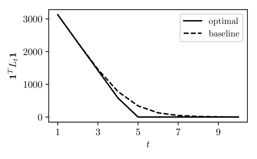
(a) Total gross liability.

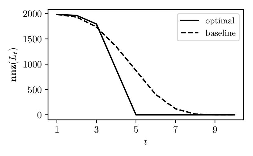
(b) Number of non-cleared liabilities.

Figure 1: Minimizing the sum of total gross liabilities. The solid line is the optimal payment schedule. The dashed line is the pro-rata baseline method.

The first stage cost function we consider is

$$g_{t}(c_{t},L_{t},P_{t})=\mathbf{1}^{T}L_{t}\mathbf{1},$$

the total gross liability at each time $t$. We compare the solution to the liability control problem (8) using this stage cost function with the pro-rata baseline method described in §4.5. The total gross liability and the number of non-cleared liabilities at each step of both sequences of payments are shown in figure 1. The optimal sequence of payments clears the liabilities by $t=5$, while the baseline clears them by $t=8$.

Risk-weighted liability.

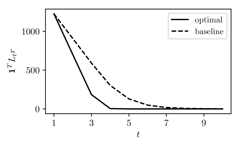
(a) Risk-weighted liability.

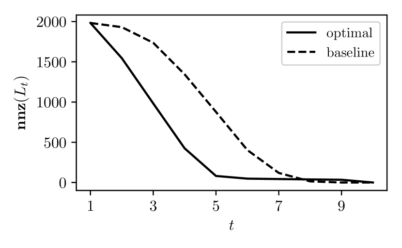
(b) Number of non-cleared liabilities.

Figure 2: Minimizing the sum of risk-weighted liabilities. The solid line is the optimal payment schedule. The dashed line is the pro-rata baseline method.

Suppose we believe that the risk of each entity is proportional to $r=\exp(-w_{1})$, where $\exp$ is taken elementwise, i.e., higher net worth implies lower risk. A reasonable stage cost function is then risk-weighted liability

$$g_{t}(c_{t},L_{t},P_{t})=\mathbf{1}^{T}L_{t}r.$$

This stage cost encourages clearing the liabilities for high risk entities before low risk entities. We compare the solution to the liability control problem (8) using this stage cost function with the pro-rata baseline method in §4.5. The total gross liability and the number of non-cleared liabilities at each step of both sequences of payments are shown in figure 2. We observe that the liabilities are still cleared by $t=5$, but the liabilities are much sparser, since the liabilities of high risk entities are cleared before those of low risk entities. We also note that the optimal payment sequence is much faster at reducing risk than the baseline.

Total squared gross payment.

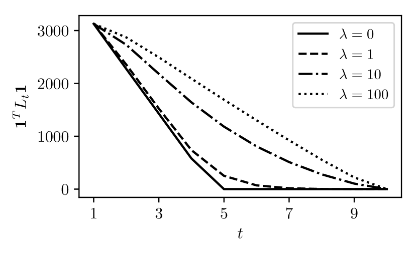
(a) Total gross liability.

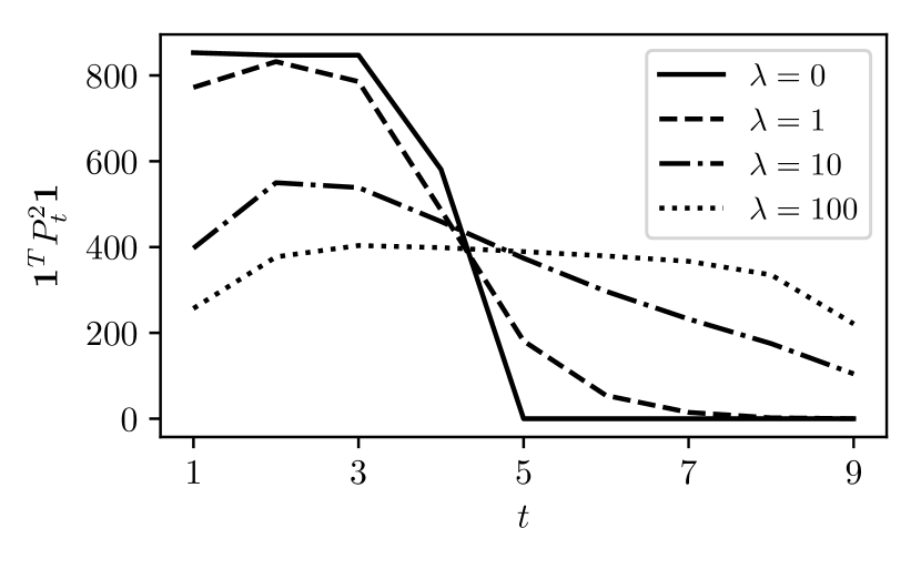
(b) Total squared gross payment.

Figure 3: Minimizing the sum of total gross liability plus total squared gross payment for various values of $\lambda$.

To the total gross liability stage cost above, we add the total squared payments, resulting in the stage cost

$$g_{t}(c_{t},L_{t},P_{t})=\mathbf{1}^{T}L_{t}\mathbf{1}+\lambda\mathbf{1}^{T}P_{t}^{2}\mathbf{1},$$

where $\lambda>0$ is a parameter. This choice of stage cost penalizes large payments, and stretches the liability clearing over a longer period of time. (We retain, however, the liability clearing constraint $L_{T}=0$.) We plot the optimal total gross liability and the total squared gross payment for various values of $\lambda$ in figure 3. (We do not compare to the pro-rata baseline because it does not seek to make payments small.)

6.2 Liability reduction

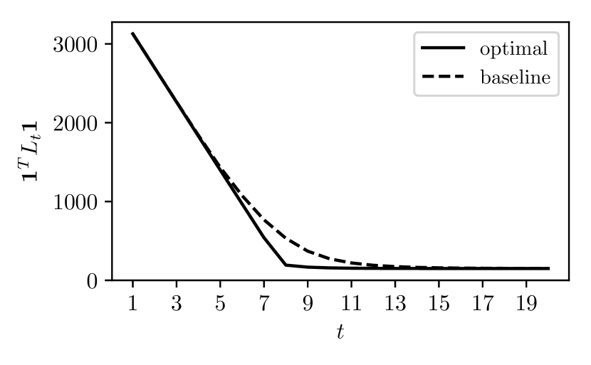
(a) Total gross liability.

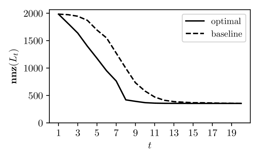
(b) Number of non-cleared liabilities.

Figure 4: Liability reduction example.

Suppose that some entities have negative initial net worth. This means that we will not be able to clear all of the liabilities; our goal is then to reduce the liabilities as much as possible, subject to the pro-rata constraint $\mathop{\bf diag}(L^{\mathrm{init}}\mathbf{1})L_{T}=\mathop{\bf diag}(L_{T}\mathbf{1})L^{\mathrm{init}}$. We consider the same liability matrix as §6.1, but change the initial cash to

$$c_{1}=\max(L^{\mathrm{init}}\mathbf{1}-(L^{\mathrm{init}})^{T}\mathbf{1}+z,0),\quad z_{i}\sim\mathcal{U}(-5,5),\quad i=1,\ldots,n,$$ (17)

where $\mathcal{U}(-5,5)$ is the uniform distribution on $[-5,5]$, which in our case leads to 49 entities with negative net worth. We consider the stage costs

$$g_{t}(c_{t},L_{t},P_{t})=\begin{cases}\mathbf{1}^{T}L_{t}\mathbf{1}&P_{t}\mathbf{1}\leq c_{t}/2,\\ +\infty&\text{otherwise},\end{cases}\quad g_{T}(c_{T},L_{T})=\mathbf{1}^{T}L_{T}\mathbf{1}.$$

The stage cost is the total gross liability, plus the indicator function of the constraint that each entity pays out no more than half of its available cash in each time period. We adjust the pro-rata baseline to

$$P_{t}=\min(\mathop{\bf diag}(c_{t}/2)\Pi,L_{t}),$$

so that each entity pays no more than half its available cash, and increase the time horizon to $T=20$. The results are displayed in figure 4. The optimal scheme is able to reduce the liabilities faster than the baseline; both methods clear all but around 350 of the original 2000 liabilities. (In §7.5 we will see an extension that directly includes the number of non-cleared liabilities in the stage cost.)

6.3 Exogenous unknown inputs

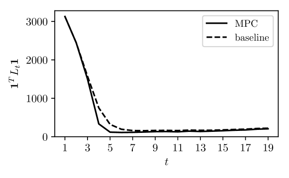
Figure 5: Liability control with exogenous inputs.

Next we consider the case where there are exogenous unknown inputs to the dynamics. The cash flows and change in liabilities are sampled according to

$$w_{t}=z_{1},\quad(W_{t})_{ij}=\begin{cases}z_{2}/10&(L^{\mathrm{init}})_{ij}>0,\\ 0&\text{otherwise},\end{cases}\quad t=1,\ldots,T-1,$$

where $\log(z_{1})\sim\mathcal{N}(0,I)$ and $\log(z_{2})\sim\mathcal{N}(0,1)$. At each time step $t$, we use the mean of the future inputs as the forecast, or

$$\hat{w}_{\tau\mid t}=e^{1/2}\mathbf{1},\quad\hat{W}_{\tau\mid t}=\begin{cases}e^{1/2}/10&(L^{\mathrm{init}})_{ij}>0,\\ 0&\text{otherwise},\end{cases}\quad\tau=t+1,\ldots,T-1.$$

We sample the initial cash vector according to

$$c_{1}=\max(L^{\mathrm{init}}\mathbf{1}-(L^{\mathrm{init}})^{T}\mathbf{1}+z,0),\quad z_{i}\sim\mathcal{U}(-5,0),\quad i=1,\ldots,n.$$

We use the stage cost function $g_{t}(c_{t},L_{t},P_{t})=\mathbf{1}^{T}L_{t}\mathbf{1}$ and the MPC policy described in §5.2. We compared the shrinking horizon MPC policy with the (modified) pro-rata baseline policy described in §5.2. The results are displayed in figure 5; note that the total gross liability appears to reach a statistical steady state and the liabilities can never be fully cleared. The MPC policy appears to be better than the baseline at reducing liabilities.

7 Extensions and variations

In this section we mention some extensions and variations on the formulations described above.

7.1 Bailouts

We can add an additional term to the dynamics that injects cash into the entities at various times, with presumably very high cost in the objective. With a linear objective term with sufficiently high weight, the bailout cash injections are zero, if it is possible to clear the liabilities without cash injection. We note that bailouts have been considered in [CC15, §2.2].

7.2 Minimum time to clear liabilities

Instead of the time-separable cost function given in (8), we take as the objective the number of steps needed to clear all liabilities. That is, our objective is $T^{\mathrm{clr}}$, defined as the minimum value of $t$ for which $L_{t}=0$ is feasible. It is easily shown that $T^{\mathrm{clr}}$ is a quasi-convex function of the liability sequence $L_{1},\ldots,L_{T}$ [BV04, §4.2.5], so this problem is readily solved using bisection, solving no more than $\log_{2}T$ convex problems. If the liabilities cannot be cleared in up to $T$ steps then we can find a $T$ such that they can be cleared using the techniques described in [AB20, §3].

7.3 Non-time-separable cost

The cost function in our basic formulation (8) is separable, i.e., a sum of terms for each $t=1,\ldots,T$. This can be extended to include non-separable cost functions. We describe a few of these below. They are convex, but non-convex versions of the same objectives can also be employed, at the cost of computational efficiency to solve the problem globally.

Smooth payments.

Adding the term $\sum_{t=2}^{T-1}\|P_{t}-P_{t-1}\|_{F}^{2}$ to the cost, where $\|A\|_{F}$ is the Frobenius norm, i.e., the square root of the sum of the squared entries of $A$, causes smooth transitions in the payment matrix. This cost is sometimes called the Dirichlet energy [BV18, §7.3] or a Laplacian regularization term [BLM90].

Piecewise constant payments.

Adding the term $\sum_{t=2}^{T-1}\|P_{t}-P_{t-1}\|_{1}$, where $\|A\|_{1}$ is the sum of absolute values of the entries of $A$, to the cost encourages the payment matrix to change in as few entries as possible between time steps. This cost is sometimes called the total variation penalty [ROF92].

Global payment restructuring.

Adding the term $\sum_{t=2}^{T-1}\|P_{t}-P_{t-1}\|_{F}$ to the cost encourages the entire payment matrix to change at as few time steps as possible [DWW14].

Per-entity payment restructuring.

Adding the term $\sum_{t=2}^{T-1}\sum_{i=1}^{n}\|P_{t}^{T}e_{i}-P_{t-1}^{T}e_{i}\|_{2}$, where $e_{i}$ is the $i$th unit vector, to the cost encourages the rows of the payment matrix, i.e., the payments made by each entity, to change at as few time steps as possible. This penalty is sometimes called a group lasso penalty [YL06].

7.4 Infinite time liability control

In §5.2 we described what is often called shrinking horizon control, because at time period $t$, we solve for a sequence of payments $P_{t},\ldots,P_{T-1}$ over the remaining horizon; the number of payments we optimize over (i.e., $T-t$) shrinks as $t$ increases. This formulation assumes there is a fixed horizon $T$.

It is also possible to consider a formulation with no fixed horizon $T$; the liability clearing is done over periods $t=1,2,\ldots$ without end. The exogenous inputs $w_{t}$ and $W_{t}$ also continue without end. Since we have exogenous inputs, we will generally not be able to clear the liabilities; our goal is only to keep the liabilities small, while making if possible small payments. In this case we have a traditional infinite horizon control or regulator problem. In economics terms, this is an equilibrium payment scheme.

The MPC formulation is readily extended to this case, and is sometimes called receding horizon control (RHC), since we are always planning out $T$ steps from the current time $t$. It is common to add a clearing constraint at the horizon in infinite time MPC or RHC formulations [RM09, §2.2].

7.5 Minimizing the number of non-cleared liabilities

Another reasonable objective to consider is the number of non-cleared (i.e., remaining) liabilities. In this case, the only cost is the number of nonzero entries in $L_{T}$. This problem is non-convex, but it can be readily formulated as a mixed-integer convex program (MICP), and solved, albeit slowly, using standard MICP techniques such as branch-and-bound [LD60]. It can also be approximately solved much quicker using heuristics, such as iterative weighted $\ell_{1}$-minimization [CWB08].

As a numerical example, we consider a smaller version of the initial liability matrix used in §6, with $n=40$ and 400 nonzero initial liabilities. We sample the initial cash according to (17), so that the liabilities cannot be fully cleared, and use a time horizon $T=10$. Minimizing the sum of total gross liabilities takes 0.05 seconds, resulting in 46 non-cleared liabilities and a final total gross liability of 22.52. By contrast, minimizing the number of non-cleared liabilities takes 22.93 seconds, resulting in only 10 non-cleared liabilities and a final total gross liability of 29.78. (The increase in computation time of a mixed-integer convex optimal control problem, compared to a convex optimal control problem of the same size, increases rapidly with problem size.)

As an extension of minimizing the number of non-cleared liabilities, we can consider minimizing the number of non-cleared entities. If the $i$th row of $L_{t}$ is zero, it means that entity $i$ does not owe anything to the others, and we say this entity is cleared. We can easily add the number of non-cleared entities to our stage cost, using a mixed-integer convex formulation.

7.6 Distributed algorithm

As stated, the liability control problem (8) requires global coordination, i.e., full knowledge of the cash held and the liabilities between the entities throughout the optimization procedure. In many settings where cash, liabilities, or payments cannot be publicly disclosed, this is not possible.

It is possible to solve the liability control problem in a distributed manner where each entity only knows its cash and the payments and liabilities it is involved in during the optimization procedure. That is, entity $i$ only needs to know $(c_{t})_{i}$, the $i$th row and column of $L_{t}$, and the $i$th row and column of $P_{t}$.

We can do this by adding a variable $\tilde{P}_{t}\in{\mbox{\bf R}}_{+}^{n\times n}$, the constraint $\tilde{P}_{t}=P_{t}^{T}$, $t=1,\ldots,T$, and replacing the cash dynamics (3) with

$$c_{t+1}=c_{t}-P_{t}\mathbf{1}+\tilde{P}_{t}\mathbf{1},\quad t=1,\ldots,T-1.$$

Then, by applying the alternating direction method of multipliers (ADMM) to the splitting $(c_{t},L_{t},P_{t})$ and $\tilde{P}_{t}$, we arrive at a distributed algorithm for the problem [BPC⁺11]. Each iteration of the algorithm involves three steps; 1) each entity solves a separate control problem to compute their cash, outbound liabilities, and outbound payments; 2) each entity solves a separate least squares problem that depends on their inbound payments; and 3) each entity performs a separate dual variable update. When the stage cost is convex, this algorithm is guaranteed to converge to a (global) solution [BPC⁺11, Appendix A]. Each step of the algorithm only requires coordination between entities connected in the liability graph, and hence preserves some level of privacy. Similar ideas have been used to develop distributed privacy-preserving implementations of predictive patient models across hospitals [JDVS⁺16] and energy management across microgrid systems [LGX17].

Appendix A Sparsity preserving formulation

In this section we describe a sparsity-preserving formulation of problem (8). We make use of the fact that $L_{t}$ and $P_{t}$ are at least as sparse as $L^{\mathrm{init}}$ (see §3).

First, let $m=\mathbf{nnz}(L^{\mathrm{init}})$ and $I_{k}\in\{1,\ldots,n\}\times\{1,\ldots,n\}$, $k=1,\ldots,m$, be the sparsity pattern of $L^{\mathrm{init}}$, meaning $(L^{\mathrm{init}})_{ij}=0$ for all $(i,j)\not\in I_{k}$, $k=1,\ldots,m$. Instead of working with the matrix variables $L_{t}$ and $P_{t}$, we work with the vector variables $l_{t}\in{\mbox{\bf R}}_{+}^{m}$ and $p_{t}\in{\mbox{\bf R}}_{+}^{m}$, which represent the nonzero entries of $L_{t}$ and $P_{t}$ (in the same order). That is,

$$(l_{t})_{k}=(L_{t})_{ij},\quad(p_{t})_{k}=(P_{t})_{ij},\quad(i,j)=I_{k},\quad k=1,\ldots,m.$$

The initial liability is given by $l^{\mathrm{init}}\in{\mbox{\bf R}}_{+}^{m}$, which contains the nonzero entries of $L^{\mathrm{init}}$. The sparsity preserving formulation of the optimal control problem (8) has the form

$$\begin{array}[]{ll}\mbox{minimize}&\sum_{t=1}^{T-1}g_{t}(c_{t},l_{t},p_{t})+g_{T}(c_{T},l_{T})\\ \mbox{subject to}&l_{t+1}=l_{t}-p_{t},\quad t=1,\ldots,T-1,\\ &c_{t+1}=c_{t}-S^{\mathrm{row}}p_{t}+S^{\mathrm{col}}p_{t},\quad t=1,\ldots,T-1,\\ &S^{\mathrm{row}}p_{t}\leq c_{t},\quad t=1,\ldots,T-1,\\ &p_{t}\geq 0,\quad t=1,\ldots,T-1,\\ &l_{t}\geq 0,\quad t=1,\ldots,T,\\ &c_{1}=c^{\mathrm{init}},\quad l_{1}=l^{\mathrm{init}},\quad c_{T}\geq 0,\end{array}$$ (18)

where $S^{\mathrm{row}}\in{\mbox{\bf R}}^{n\times m}$ sums the rows of $P_{t}$, i.e., $S^{\mathrm{row}}p_{t}=P_{t}\mathbf{1}$, and $S^{\mathrm{col}}\in{\mbox{\bf R}}^{n\times m}$ sums the columns of $P_{t}$, i.e., $S^{\mathrm{col}}p_{t}=P_{t}^{T}\mathbf{1}$. The cost functions are applied only to the nonzero entries of $L_{t}$ and $P_{t}$, so they take the form $g_{t}:{\mbox{\bf R}}_{+}^{n}\times{\mbox{\bf R}}_{+}^{m}\times{\mbox{\bf R}}_{+}^{m}\to{\mbox{\bf R}}\cup\{+\infty\}$ and $g_{T}:{\mbox{\bf R}}_{+}^{n}\times{\mbox{\bf R}}_{+}^{m}\to{\mbox{\bf R}}\cup\{+\infty\}$. Problem (18) has just $2T(n+m)$ variables, which can be much fewer than the original $2T(n+n^{2})$ variables when $m\ll n^{2}$.

References

- [AAB+19] Akshay Agrawal, Brandon Amos, Shane Barratt, Stephen Boyd, Steven Diamond, and J Zico Kolter. Differentiable convex optimization layers. In Advances in Neural Information Processing Systems, pages 9558–9570, 2019.
- [AB20] Akshay Agrawal and Stephen Boyd. Disciplined quasiconvex programming. Optimization Letters, pages 1–15, 2020.
- [AG00] Franklin Allen and Douglas Gale. Financial contagion. Journal of Political Economy, 108(1):1–33, 2000.
- [aps20] MOSEK optimization suite. https://www.mosek.com, 2020.
- [AVDB18] Akshay Agrawal, Robin Verschueren, Steven Diamond, and Stephen Boyd. A rewriting system for convex optimization problems. Journal of Control and Decision, 5(1):42–60, 2018.
- [BAS10] Lars Blackmore, Behçet Açikmeşe, and Daniel Scharf. Minimum-landing-error powered-descent guidance for Mars landing using convex optimization. Journal of Guidance, Control, and Dynamics, 33(4):1161–1171, 2010.
- [BBD+17] Stephen Boyd, Enzo Busseti, Steven Diamond, Ronald Kahn, Kwangmoo Koh, Peter Nystrup, and Jan Speth. Multi-period trading via convex optimization. Foundations and Trends® in Optimization, 3(1):1–76, 2017.
- [BBF18] Tathagata Banerjee, Alex Bernstein, and Zachary Feinstein. Dynamic clearing and contagion in financial networks. arXiv preprint arXiv:1801.02091, 2018.
- [Bem06] Alberto Bemporad. Model predictive control design: New trends and tools. In IEEE Conference on Decision and Control, pages 6678–6683, 2006.
- [BEST04] Michael Boss, Helmut Elsinger, Martin Summer, and Stefan Thurner. Network topology of the interbank market. Quantitative Finance, 4(6):677–684, 2004.
- [BF19] Tathagata Banerjee and Zachary Feinstein. Impact of contingent payments on systemic risk in financial networks. Mathematics and Financial Economics, 13(4):617–636, 2019.
- [BFVY19] Marco Bardoscia, Gerardo Ferrara, Nicholas Vause, and Michael Yoganayagam. Full payment algorithm. Available at SSRN, 2019.
- [BH12] Geert Bekaert and Robert Hodrick. International Financial Management. Pearson Education, 2 edition, 2012.
- [BLM90] Jan Biemond, Reginald Lagendijk, and Russell Mersereau. Iterative methods for image deblurring. Proceedings of the IEEE, 78(5):856–883, 1990.
- [Boa20] Board of Governors of the Federal Reserve System. Reserve requirements. https://www.federalreserve.gov/monetarypolicy/reservereq.htm, March 2020.
- [BPC+11] Stephen Boyd, Neal Parikh, Eric Chu, Borja Peleato, Jonathan Eckstein, et al. Distributed optimization and statistical learning via the alternating direction method of multipliers. Foundations and Trends® in Machine learning, 3(1):1–122, 2011.
- [Bro09] Derk Brouwer. System and method of implementing massive early terminations of long term financial contracts, 2009. US Patent 7,613,649.
- [BV04] Stephen Boyd and Lieven Vandenberghe. Convex Optimization. Cambridge University Press, 2004.
- [BV18] Stephen Boyd and Lieven Vandenberghe. Introduction to Applied Linear Algebra: Vectors, Matrices, and Least Squares. Cambridge University Press, 2018.
- [CC15] Agostino Capponi and Peng-Chu Chen. Systemic risk mitigation in financial networks. Journal of Economic Dynamics and Control, 58:152–166, 2015.
- [CFS05] Rodrigo Cifuentes, Gianluigi Ferrucci, and Hyun Song Shin. Liquidity risk and contagion. Journal of the European Economic Association, 3(2-3):556–566, 2005.
- [CTHK03] Eunkyoung Cho, Kristin Thoney, Thom Hodgson, and Russell King. Supply chain planning: Rolling horizon scheduling of multi-factory supply chains. In Proc. Conference on Winter Simulation: Driving Innovation, pages 1409–1416, 2003.
- [CWB08] Emmanuel Candes, Michael Wakin, and Stephen Boyd. Enhancing sparsity by reweighted minimization. Journal of Fourier Analysis and Applications, 14(5-6):877–905, 2008.
- [DB16] Steven Diamond and Stephen Boyd. CVXPY: A Python-embedded modeling language for convex optimization. Journal of Machine Learning Research, 17(83):1–5, 2016.
- [DD83] Douglas Diamond and Philip Dybvig. Bank runs, deposit insurance, and liquidity. Journal of Political Economy, 91(3):401–419, 1983.
- [DR17] Marco D’Errico and Tarik Roukny. Compressing over-the-counter markets. Technical report, European Systemic Risk Board, 2017.
- [DWW14] Patrick Danaher, Pei Wang, and Daniela Witten. The joint graphical lasso for inverse covariance estimation across multiple classes. Journal of the Royal Statistical Society: Series B (Statistical Methodology), 76(2):373–397, 2014.
- [Els09] Helmut Elsinger. Financial networks, cross holdings, and limited liability. Working Papers, Oesterreichische Nationalbank (Austrian Central Bank), (156), 2009.
- [EN01] Larry Eisenberg and Thomas Noe. Systemic risk in financial systems. Management Science, 47(2):236–249, 2001.
- [FBA+07] Paolo Falcone, Francesco Borrelli, Jahan Asgari, Hongtei Tseng, and Davor Hrovat. Predictive active steering control for autonomous vehicle systems. IEEE Transactions on Control Systems Technology, 15(3):566–580, 2007.
- [Fed19] Federal Deposit Insurance Corporation. Statistics at a glance. https://www.fdic.gov/bank/statistical/stats/2019dec/industry.pdf, December 2019.
- [Fei19] Zachary Feinstein. Obligations with physical delivery in a multilayered financial network. SIAM Journal on Financial Mathematics, 10(4):877–906, 2019.
- [FNB19] Anqi Fu, Balasubramanian Narasimhan, and Stephen Boyd. CVXR: An R package for disciplined convex optimization. In Journal of Statistical Software, 2019.
- [FPR+18] Zachary Feinstein, Weijie Pang, Birgit Rudloff, Eric Schaanning, Stephan Sturm, and Mackenzie Wildman. Sensitivity of the Eisenberg–Noe clearing vector to individual interbank liabilities. SIAM Journal on Financial Mathematics, 9(4):1286–1325, 2018.
- [FRW17] Zachary Feinstein, Birgit Rudloff, and Stefan Weber. Measures of systemic risk. SIAM Journal on Financial Mathematics, 8(1):672–708, 2017.
- [GB08] Michael Grant and Stephen Boyd. Graph implementations for nonsmooth convex programs. In Recent Advances in Learning and Control, Lecture Notes in Control and Information Sciences, pages 95–110. Springer-Verlag Limited, 2008.
- [GB14] Michael Grant and Stephen Boyd. CVX: Matlab software for disciplined convex programming, version 2.1, 2014.
- [GY15] Paul Glasserman and H Young. How likely is contagion in financial networks? Journal of Banking & Finance, 50:383–399, 2015.
- [HR55] Theodore Harris and Fiona Ross. Fundamentals of a method for evaluating rail net capacities. Technical report, RAND Corp, Santa Monica, CA, 1955.
- [JDVS+16] Arthur Jochems, Timo M Deist, Johan Van Soest, Michael Eble, Paul Bulens, Philippe Coucke, Wim Dries, Philippe Lambin, and Andre Dekker. Distributed learning: developing a predictive model based on data from multiple hospitals without data leaving the hospital–a real life proof of concept. Radiotherapy and Oncology, 121(3):459–467, 2016.
- [Kah62] Arthur Kahn. Topological sorting of large networks. Communications of the ACM, 5(11):558–562, 1962.
- [KP19] Aein Khabazian and Jiming Peng. Vulnerability analysis of the financial network. Management Science, 65(7):3302–3321, 2019.
- [KV19] Michael Kusnetsov and Luitgard Veraart. Interbank clearing in financial networks with multiple maturities. SIAM Journal on Financial Mathematics, 10(1):37–67, 2019.
- [LD60] Alisa Land and Alison Doig. An automatic method of solving discrete programming problems. Econometrica, 28(3):497–520, 1960.
- [LGX17] Yun Liu, Hoay Beng Gooi, and Huanhai Xin. Distributed energy management for the multi-microgrid system based on admm. In Power & Energy Society General Meeting, pages 1–5. IEEE, 2017.
- [Lof04] Johan Lofberg. YALMIP: A toolbox for modeling and optimization in MATLAB. In IEEE International Conference on Robotics and Automation, pages 284–289. IEEE, 2004.
- [MB09] Jacob Mattingley and Stephen Boyd. Automatic code generation for real-time convex optimization. Convex Optimization in Signal Processing and Communications, pages 1–41, 2009.
- [MB12] Jacob Mattingley and Stephen Boyd. CVXGEN: A code generator for embedded convex optimization. Optimization and Engineering, 13(1):1–27, 2012.
- [MBBW19] Nicholas Moehle, Enzo Busseti, Stephen Boyd, and Matt Wytock. Dynamic energy management. In Large Scale Optimization in Supply Chains and Smart Manufacturing, pages 69–126. Springer, 2019.
- [MBH+11] Yudong Ma, Francesco Borrelli, Brandon Hencey, Brian Coffey, Sorin Bengea, and Philip Haves. Model predictive control for the operation of building cooling systems. IEEE Transactions on Control Systems Technology, 20(3):796–803, 2011.
- [MWB11] Jacob Mattingley, Yang Wang, and Stephen Boyd. Receding horizon control. IEEE Control Systems Magazine, 31(3):52–65, 2011.
- [O’K14] Dominic O’Kane. Optimizing the compression cycle: algorithms for multilateral netting in OTC derivatives markets. Available at SSRN 2273802, 2014.
- [O’K17] Dominic O’Kane. Optimising the multilateral netting of fungible OTC derivatives. Quantitative Finance, 17(10):1523–1534, 2017.
- [RM09] James Rawlings and David Mayne. Model Predictive Control: Theory and Design. Nob Hill Publishing, 2009.
- [ROF92] Leonid Rudin, Stanley Osher, and Emad Fatemi. Nonlinear total variation based noise removal algorithms. Physica D: Nonlinear Phenomena, 60(1-4):259–268, 1992.
- [RV13] Leonard Rogers and Luitgard Veraart. Failure and rescue in an interbank network. Management Science, 59(4):882–898, 2013.
- [Sha78] Alan Shapiro. Payments netting in international cash management. Journal of International Business Studies, 9(2):51–58, 1978.
- [SS19] Steffen Schuldenzucker and Sven Seuken. Portfolio compression in financial networks: Incentives and systemic risk. Available at SSRN, 2019.
- [SWBB11] Mohsen Soltani, Rafael Wisniewski, Per Brath, and Stephen Boyd. Load reduction of wind turbines using receding horizon control. In IEEE International Conference on Control Applications, pages 852–857. IEEE, 2011.
- [UMZ+14] Madeleine Udell, Karanveer Mohan, David Zeng, Jenny Hong, Steven Diamond, and Stephen Boyd. Convex optimization in Julia. Workshop on High Performance Technical Computing in Dynamic Languages, 2014.
- [Ver19] Luitgard Veraart. When does portfolio compression reduce systemic risk? Available at SSRN 3488398, 2019.
- [WB09] Yang Wang and Stephen Boyd. Performance bounds for linear stochastic control. Systems & Control Letters, 58(3):178–182, 2009.
- [YL06] Ming Yuan and Yi Lin. Model selection and estimation in regression with grouped variables. Journal of the Royal Statistical Society: Series B (Statistical Methodology), 68(1):49–67, 2006.