Holographic QFTs on S${}^{2}\times$S², spontaneous symmetry breaking and Efimov saddle points

Abstract:

Holographic CFTs and holographic RG flows on space-time manifolds which are $d$-dimensional products of spheres are investigated. On the gravity side, this corresponds to Einstein-dilaton gravity on an asymptotically $AdS_{d+1}$ geometry, foliated by a product of spheres. We focus on holographic theories on $S^{2}\times S^{2}$, we show that the only regular five-dimensional bulk geometries have an IR endpoint where one of the sphere shrinks to zero size, while the other remains finite. In the $Z_{2}$-symmetric limit, where the two spheres have the same UV radii, we show the existence of a infinite discrete set of regular solutions, satisfying an Efimov-like discrete scaling. The $Z_{2}$-symmetric solution in which both spheres shrink to zero at the endpoint is singular, whereas the solution with lowest free energy is regular and breaks $Z_{2}$ symmetry spontaneously. We explain this phenomenon analytically by identifying an unstable mode in the bulk around the would-be $Z_{2}$-symmetric solution. The space of theories have two branches that are connected by a conifold transition in the bulk, which is regular and correspond to a quantum first order transition. Our results also imply that $AdS_{5}$ does not admit a regular slicing by $S^{2}\times S^{2}$.

1 Introduction, summary of results and outlook

Quantum field theories are usually studied in flat background space-time. We can consider them, however, in background space-times that have non-trivial curvature. Space-time curvature is irrelevant in the UV, as at short distances any regular manifold is essentially flat. However, curvature is relevant in the IR and affects importantly the low-energy structure of the QFT.

There are several motivations to consider QFT in curved backgrounds.

• Many computations in CFTs and other massless QFTs (like that of supersymmetric indices) are well-defined when a (controllable) mass gap is introduced, and this can be generated by putting the theory on a positive curvature manifold, like a sphere. This has been systematically used in calculating supersymmetric indices in CFTs, [1] as well as regulating IR divergences of perturbation theory in QFT, [2, 3, 4] and string theory, [5].

• Partition functions of QFTs on compact manifolds, like spheres, are important ingredients in the study of the monotonicity of the RG Flow and the definition of generalized C-functions, especially in odd dimensions, [6, 7, 8].

• Cosmology has always given a strong motivation to study QFT in curved space-time, [9, 10]. Especially, QFT in de Sitter or almost de Sitter space is motivated by early universe inflation as well as the current acceleration of the universe.

• The issue of quantum effects in near de Sitter backgrounds is a controversial issue even today, [11]-[15].

• Partition functions of holographic QFTs on curved manifolds are important ingredients in the no-boundary proposal of the wave-function of the universe, [16], and serve to determine probabilities for various universe geometries.

• Curvature in QFT, although UV-irrelevant is IR-relevant and can affect importantly the IR physics. Among other, things it can drive (quantum) phase transitions in the QFT, [17].

• Putting holographic QFTs on curved manifolds potentially leads to constant (negative) curvature metrics sliced by curved slices. The Fefferman-Graham theorem guarantees that such regular metrics exist near the asymptotically AdS boundary, [18]. However, it is not clear whether such solutions can be extended to globally regular solutions in the Euclidean case (which may have horizons in Minkowski signature). The few facts that are known can be found in [19, 20].

  Using holography, it may be argued, that as we can put any holographic CFT on any manifold we choose, there should be a related regular solution that is dual to such a saddle point. This quick argument has however a catch: it may be that for a regular solution to exist, more of the bulk fields need to be turned-on (spontaneously), via asymptotically vev solutions. We shall see in this paper, a milder version of this phenomenon associated with spontaneous symmetry breaking of a parity-like $Z_{2}$ symmetry.

In this paper we are going to pursue a research program started in [21] and [17], that investigates the general structure of holographic RG flows for QFTs defined on various spaces that involve beyond flat space, constant curvature manifolds. The cases analysed so far systematically concern the flat space case (or equivalently $(S^{1})^{d}$), and the $S^{d}$, $dS_{d}$ and $AdS_{d}$ cases, although the results in [17, 8, 15] are valid for any d-dimensional Einstein manifold.

The case of $S^{1}\times S^{d-1}$ has also been studied extensively as it contains $AdS_{d+1}$ in global coordinates, and RG flows were also analysed in this case. The general problem we are now interested in, is the case where the boundary is a product of constant (positive) curvature manifolds, which we shall take without a loss of generality to be spheres.

In the CFT case, unlike the $S^{d}$ and $S^{1}\times S^{d-1}$ cases, there is no known slicing of $AdS_{d+1}$ by other sphere product manifolds , and even in this cases the solutions if they are regular must be non-trivial.

Solutions for CFTs on sphere product manifolds have been recently investigated in [22] and phases transitions were found, generalizing the Hawking-Page transition (that is relevant in the $S^{1}\times S^{d-1}$ case), [23].

In this work, we study four-dimensional holographic QFTs on $S^{2}\times S^{2}$. The QFTs we shall consider are either CFTs, or RG-flows driven by a single scalar operator $O$ of dimension $\Delta$.

We shall describe the dual theory in the bulk, in terms of five-dimensional Einstein-dilaton gravity. The relevant geometries, describing the ground-state of the theory, are then asymptotically $AdS_{5}$ space-times which admit a radial $S^{2}\times S^{2}$ foliation. In the case of CFTs, these space-times are solution of pure gravity with a negative cosmological constant. In the case of RG flows, these are solutions of Einstein-dilaton gravity with an appropriate scalar potential.

The geometry $S^{2}\times S^{2}$ is the only four-dimensional sphere product manifold which has not been already studied in detail. It is also the only one that, as we shall see, cannot be used to slice the AdS₅ metric.

Below, we briefly summarize our setup and our main results.

We consider geometries whose metric is of the form:

$$ds^{2}=du^{2}+e^{2A_{1}(u)}\alpha_{1}^{2}d\Omega_{1}^{2}+e^{2A_{2}(u)}\alpha_{2}^{2}d\Omega_{2}^{2}$$ (1.1)

where $\alpha_{1}$ and $\alpha_{2}$ are constants with dimensions of length, and $d\Omega_{i}^{2}$ are the metrics of $S^{2}$s with radius 1. The generic space-time symmetry of the QFT, is $SU(2)\times SU(2)$ associated with the two spheres. When the spheres have equal size, $\alpha_{1}=\alpha_{2}$, then we have an extra $Z_{2}$ space-time symmetry that interchanges the two spheres.

The holographic coordinate $u$ in (1.1) runs from the conformal boundary at $u=-\infty$, corresponding to a UV fixed-point of the dual QFT, to an IR endpoint $u_{0}$ where the manifold ends regularly.

The UV geometry and parameters.

In the near-boundary region, the space-time asymptotes $AdS_{5}$ with length-scale $\ell$. The metric on the boundary is (with an appropriate definition of the scale factors) conformally equivalent to the four-dimensional metric

$$ds_{bdr}^{2}=\alpha_{1}^{2}d\Omega_{1}^{2}+\alpha_{2}^{2}d\Omega_{2}^{2}$$ (1.2)

This is the metric on the $S^{2}\times S^{2}$ manifold on which the dual UV field theory is defined. Near the boundary, the scalar field behaves at leading order as

$$\varphi\simeq\left(\varphi_{-}\ell^{\Delta_{-}}\right)\,e^{\Delta_{-}u/\ell}+\ldots\qquad u\to-\infty$$ (1.3)

where $\varphi_{-}$ is a constant, $\ell$ the $AdS_{5}$ length, and $\Delta_{-}=4-\Delta>0$.

The UV theory is defined in terms of three sources, entering equations (1.2-1.3):

• The scalar source $\varphi_{-}$ dual to the relevant coupling deforming the UV CFT;

• The radii $\alpha_{1}$ and $\alpha_{2}$ of the two spheres, or equivalently their scalar curvatures $R_{i}^{UV}\equiv 2/\alpha_{i}^{2}$.

They can be combined into two dimensionless parameters,

$${\mathcal{R}}_{1}={R_{1}^{UV}\over\varphi_{-}^{2/\Delta_{-}}},\quad{\mathcal{R}}_{2}={R_{2}^{UV}\over\varphi_{-}^{2/\Delta_{-}}}.$$ (1.4)

At subleading order in the UV expansions one finds two more dimensionless integration constants of the bulk field equations, that we denote $C_{1}$ and $C_{2}$ and are related to vevs of the field theory operators. Schematically, they enter the scalar field and the scale factors in the following way:

$$A_{1}\sim\ldots+C_{1}e^{4u/\ell}+\ldots,\quad A_{2}\sim\ldots+C_{2}e^{4u/\ell}+\ldots$$ (1.5)

$$\varphi\sim\ldots+(C_{1}+C_{2})e^{(4-\Delta_{-})u/\ell}+\ldots$$ (1.6)

• The combination $C_{1}+C_{2}$ sets the vacuum expectation value of the scalar field dual to $\varphi$,

  $$\langle O\rangle\propto\varphi_{-}^{\Delta/\Delta_{-}}(C_{1}+C_{2})$$ (1.7)

  This combination also enters in the expectation value of the trace of the stress tensor.

• The combination $C_{1}-C_{2}$ enters at order $e^{4u/\ell}$ in the difference of the scale factors,

  $$A_{1}-A_{2}=\ldots+(C_{1}-C_{2})e^{4u/\ell}+\ldots\qquad u\to-\infty$$ (1.8)

  and it enters the difference in the stress tensor vevs along the two spheres.

• Additional terms in the stress tensor vev come from the curvatures $\mathcal{R}_{i}$, and they reproduce in particular the Weyl anomaly on $S^{2}\times S^{2}$.

• In the limit where the source $\varphi_{-}\to 0$, one can find “pure vev” solutions, in which the leading asymptotics of the scalar field are

  $$\varphi\simeq\left(\varphi_{+}\ell^{\Delta}\right)e^{\Delta u/\ell}+\ldots,\qquad u\to-\infty$$ (1.9)

  In this case, only the combination $C_{1}-C_{2}$ is allowed to be non-zero, and the scalar vev parameter $C_{1}+C_{2}$ is replaced by the constant parameter $\varphi_{+}$. These solutions are dual to vev-driven flows: the source of the operator dual to $\varphi$ is set to zero, but a non-zero condensate triggers a non-trivial RG flow. These solutions have one free parameter less than the source-driven flows, therefore, they are generically singular in the IR unless the bulk potential is appropriately fine-tuned [17, 24].

IR Geometry.

Regular solutions of the form (1.1) have an IR endpoint at some finite $u=u_{0}$, where the geometry has the following properties:

• At the endpoint, one of the two scale factors $e^{A_{i}(u_{0})}$ vanishes, and the corresponding sphere shrinks to zero size, while the other sphere stays at finite size. Near $u_{0}$, the metric has the form

  $$ds^{2}\simeq du^{2}+(u-u_{0})^{2}d\Omega_{1}^{2}+\alpha_{IR}^{2}d\Omega_{2}^{2},$$ (1.10)

  and the geometry is isometric to $R^{3}\times S^{2}$. Therefore the topology of the solution is that of $D_{3}\times S^{2}$ where $D_{3}$ is a “cigar” with $S^{2}$ slices or equivalently a hemisphere of an $S^{3}$. Instead, any solution in which the two spheres shrink to zero at the same point, has necessarily a curvature singularity.

• Regularity imposes two constraints on the four dimensionless UV parameters $\mathcal{R}_{1},\mathcal{R}_{2},C_{1},C_{2}$. Choosing the sources $\mathcal{R}_{1},\mathcal{R}_{2}$ as independent free parameters, regularity fixes the vevs $C_{1},C_{2}$ as a function of the sources, as it always happens in holography:

  $$C_{1,2}=C_{1,2}(\mathcal{R}_{1},\mathcal{R}_{2})$$ (1.11)

• From an analysis of the quadratic curvature invariants, we show that no regular slicing of Euclidean $AdS_{5}$ by $S^{2}\times S^{2}$ exists (unlike the known slicing by $S^{1}\times S^{3}$, which corresponds to $AdS_{5}$ in global coordinates, and by $S^{4}$, discussed in [17]). Instead, it is possible to find a regular slicing of $AdS_{5}$ by $AdS_{2}\times S^{2}$.

Efimov spiral and spontaneous $\mathbb{Z}_{2}$ breaking.

If the UV radii of the two spheres are very different, there is a single regular solution, in which it is the sphere with the smallest UV radius that shrinks to zero size in the IR. As the UV curvatures become comparable however, multiple solutions start appearing with one or the other sphere shrinking to zero in the IR.

The limit in which $\mathcal{R}_{1}=\mathcal{R}_{2}$ is particularly interesting. In this case, the two spheres start with the same size in the UV, and the theory has a space-time $\mathbb{Z}_{2}$ symmetry under which the two spheres are interchanged.

However, this symmetry is broken by the dynamics. This is seen in the gravitational solution where in the bulk, the symmetric solution, in which $A_{1}(u)=A_{2}(u)$ all the way to the IR endpoint, is singular, as we have discussed above. Any regular solution must therefore break the $\mathbb{Z}_{2}$ symmetry by the presence of a non-zero vev parameter $C_{1}-C_{2}$, which causes $A_{1}(u)-A_{2}(u)$ to depart from zero as we move away from the boundary, as in equation (1.8). This is similar to what happens with the singular conifold in the Klebanov-Strassler solution [25], where the non-zero vev which avoids the singularity, is associated to gaugino condensation. In our case however, it corresponds to the spontaneous breaking of a discrete space-time symmetry.

This is indeed what happens: as $\mathcal{R}_{1}/\mathcal{R}_{2}\to 1$, the theory develops an infinite discrete set of regular solutions, characterized by a smaller and smaller IR radius $\alpha_{IR}$ of the finite $S^{2}$, which approaches the singular solution characterized by $\alpha_{IR}=0$ and $C_{1}=C_{2}$. In this regime, the solutions follow a discrete scaling law well described by an Efimov spiral in the plane $(\mathcal{R}_{1}/\mathcal{R}_{2},C_{1}-C_{2})$, given schematically by:

$${\mathcal{R}_{2}\over\mathcal{R}_{1}}-1=A\sin(s+\phi_{1})e^{-bs},\qquad C_{1}-C_{2}=B\sin(s+\phi_{2})e^{-bs}$$ (1.12)

where $A,B$, $b$ and $\phi_{1},\phi_{2}$ are constants, and $s\sim\log(\ell/\alpha_{IR})$ runs to infinity in the singular limit. The schematic behavior is shown in figure 1, where each point of the spiral corresponds to a regular solution. The solutions lying on the vertical axis form an infinite countable set and correspond to a symmetric UV boundary condition $\mathcal{R}_{1}=\mathcal{R}_{2}$. The center of the spiral corresponds to the singular solution with $\mathcal{R}_{1}=\mathcal{R}_{2}$ and $C_{1}=C_{2}$.

\begin{overpic}[width=281.85034pt]{Figures/spiral-intro-3} \put(95.0,35.0){${\mathcal{R}_{1}\over\mathcal{R}_{2}}-1$} \put(50.0,85.0){$C_{1}-C_{2}$} \end{overpic}

Figure 1: Efimov spiral. Each point on the spiral represents a regular solution with sphere 1 shrinking to zero size and sphere 2 remaining finite in the IR. As we proceed towards the center, the IR radius of sphere 2 becomes smaller and smaller. The origin corresponds to the singular solution, in which both spheres shrink to zero size.

The symmetric solutions correspond to vanishing ${\mathcal{R}_{2}/\mathcal{R}_{1}}-1$ and one can find an infinite number of them at discrete values of $s$. The corresponding values of $C_{1}-C_{2}$ get smaller and smaller as $s$ grows larger.

The Efimov behavior (1.12) is confirmed by numerical examples, both in the case of a CFT (no scalar field, in which case it was already observed in [22]) and in the case of holographic RG-flows.

This type of Efimov scaling has been observed in other contexts in holography, [26, 27, 28]. For example, in holographic QCD-like theories, it is associated to a would-be IR fixed point developing an instability to a violation of the BF bound [28]. The associated symmetry that is broken is the chiral symmetry. Interestingly, a similar interpretation can be found in the present context: we show that the scale factor difference $A_{1}-A_{2}$ behaves, away from the boundary, as an unstable perturbation. This behavior can be generalized to spheres of different dimensions, as discussed in Appendix G.2

Conifold transition.

Having established that there may be multiple solutions for a given choice of the UV parameters $\mathcal{R}_{1}$ and $\mathcal{R}_{2}$ (and even an infinite number for the $\mathbb{Z}_{2}$-symmetric choice $\mathcal{R}_{1}=\mathcal{R}_{2}$) we analyse which one is the dominant saddle-point solution. For this, we compute the free energy of the regular solutions as a function of $\mathcal{R}_{1},\mathcal{R}_{2}$ by evaluating the Euclidean on-shell action. The solution with the lowest free energy at fixed $\mathcal{R}_{1},\mathcal{R}_{2}$ is the ground state of the system.

\begin{overpic}[width=281.85034pt]{Figures/spiral-intro-2} \put(95.0,45.0){${\mathcal{R}_{1}\over\mathcal{R}_{2}}-1$} \put(35.0,95.0){$C_{1}-C_{2}$} \put(85.0,90.0){$\mathcal{R}_{1}>\mathcal{R}_{2}$} \put(0.0,8.0){$\mathcal{R}_{1}<\mathcal{R}_{2}$} \end{overpic}

Figure 2: The two spirals correspond to the solutions in which sphere 1 shrinks to zero in the IR (red) and to those in which sphere 2 shrinks (blue). As we cross the vertical axis, the dominant solution jumps from the red to the blue spiral.

Both in the case of a CFT and of a non-trivial RG flow, we find that the lowest free energy corresponds to the first occurrence along the spiral of a given value of $\mathcal{R}_{1}/\mathcal{R}_{2}$, i.e. the solution which is farthest from the center.

The two dominant saddle points that exist for $\mathcal{R}_{1}=\mathcal{R}_{2}$ correspond to the dominant Efimov solutions of the two branches $\mathcal{R}_{1}>\mathcal{R}_{2}$ and $\mathcal{R}_{1}<\mathcal{R}_{2}$. They correspond to the two vacua of the theory with $\mathcal{R}_{1}=\mathcal{R}_{2}$ and they are related by the spontaneously-broken $Z_{2}$ symmetry.

If we start in the regime $\mathcal{R}_{1}>\mathcal{R}_{2}$, on the branch where sphere 1 shrinks to zero and decrease the value of $\mathcal{R}_{1}$, at the symmetric point $\mathcal{R}_{1}/\mathcal{R}_{2}=1$ the system undergoes a first order phase transition to the solution where the two spheres are interchanged: decreasing ${\mathcal{R}}_{1}$ further, the dominant branch becomes the one in which sphere 2 shrinks to zero size and sphere 1 remains finite. This transition is shown schematically in figure 2. The classical saddle point undergoes a topology-changing transition similar to the conifold transition, see figure 3. We should stress that this conifold transition occurs via regular bulk solutions, and its signal in the boundary QFT is as a first order phase transition not unlike the one in large-N YM at $\theta=\pi$, [29]. It seems to be quite distinct from the conifold transition of CY vacua in string theory, [30], where the singularity is resolved by non-perturbative effects in the string coupling.

\begin{overpic}[width=433.62pt]{Figures/topology-change} \put(35.0,48.0){Topology change} \put(46.3,3.0){1} \put(95.0,3.0){${\mathcal{R}_{2}/\mathcal{R}_{1}}$} \put(50.0,10.0){$\mathcal{R}_{1}<\mathcal{R}_{2}$} \put(30.0,10.0){$\mathcal{R}_{1}>\mathcal{R}_{2}$} \end{overpic}

Figure 3: Conifold transition. The horizontal axis represents the ratio of the UV curvatures of the two spheres. In this figure the UV radius of sphere 2 is kept fixed, while that of sphere 1 is increased going from left to right.

Outlook.

The study of holographic solutions on products of spheres can be extended to arbitrary dimension and arbitrary number of spheres. The topology changing transition has the potential applications to unveil other (known or otherwise) transitions in holography, when these can be embedded into a higher dimensional theory by the mechanism of generalized dimensional uplift [31, 32]: it is known for example that reducing a higher dimensional $AdS$ solution on a sphere yields a confining holographic theory in lower dimensions, [31]. Starting from a product of spheres can be useful to understand the phase structure of confining theories on curved manifolds.

Another interesting question from the perspective of generalized dimensional reduction/uplift is the origin of the discrete scaling discussed in this paper: here, we have identified an unstable mode underlying this phenomenon, but it would be interesting to rephrase it in terms of the more familiar language of scalar fields violating the BF bound at some IR fixed point, as it was the case in [26, 27, 28]. This formulation can be reached using the method of generalized dimensional reduction, starting from the sphere-product ansatz in higher dimensions.

Another interesting direction is to consider product manifolds which have less symmetry, for example squashed spheres. These have found a recent application in the context of cosmology, in particular in the holographic approach to the no-boundary wave function of the universe [33].

Finally, in this work we have not fully explored the case where one of the factors in the product manifold has negative curvature. Extending this work to that situation can lead to a better understanding of AdS/AdS holography, which in the case of RG flows presents some difficulty due to the appearance of conical singularities on the boundary [17]. It would be useful to understand these situations by generalized uplift to a higher dimensional AdS geometries foliated by a lower-dimensional AdS times spheres or tori.

This work is organized as follows. In Section 2, we describe in detail the setup and derive the equations of motion for holographic RG flow solutions

In section 3 we develop a first-order formalism adapted to the sphere-product ansatz, along the lines of the formalism developed in [17]. This is particularly useful for the calculation of the on-shell action.

In section 4 we discuss the UV asymptotics of the solution and identify the parameters which correspond to dual field theory quantities.

In section 5 we discuss the IR side of the geometry and we identify the conditions for the absence of singularities.

In section 6 we find the expression for the free energy, a.k.a. the on-shell action, in terms of the UV data (curvatures and vev parameters), including the appropriate holographic renormalization.

In section 7 we analyze in detail solutions in the case of a CFT: we construct solutions in numerical examples, and show that they undergo a conifold phase transition. In this section we also discuss the Efimov scaling in the CFT case, of which we give an analytical derivation in terms of an IR instability.

In section 8 we present numerical examples of the more general case of holographic RG flows on $S^{2}\times S^{2}$, where we again display the Efimov phenomenon and topology-changing transition.

Most technical details are presented in the Appendix.

Note added

During completion of this work we became aware of the article [22], which addressed similar problems and reached some of our conclusions, in the absence of a bulk scalar field.

2 Holographic Theories on S${}^{2}\times$ S²

In this section we consider the bulk holographic description of RG flows of four-dimensional QFTs on $S^{2}\times S^{2}$. But before we specialize to this, we shall first consider general holographic solutions that are cones over a general product of spheres.

As a bulk holographic theory we consider an Einstein-scalar theory in (d + 1)-dimensions with Euclidean or Lorentzian metric (in the latter case we use the mostly plus convention). The two relevant bulk fields we keep are the metric, dual to the conserved QFT energy-momentum tensor, and a scalar field $\varphi$, dual to a relevant scalar operator $O$ that is driving the RG flow of the boundary QFT. The bulk theory in the infinite coupling limit, is described by the following two-derivative action (after field redefinitions):

$$S[g,\varphi]=\int du\,d^{d}x\,\sqrt{|g|}\left(R^{(g)}-\frac{1}{2}\partial_{a}\varphi\partial^{a}\varphi-V(\varphi)\right)+S_{GHY}\,,$$ (2.1)

where we also included the Gibbons-Hawking-York term $S_{GHY}$. In the Lorentzian signature we use the $(-,+\ldots+)$ convention for the metric. The Euclidean action is defined by setting $S_{E}=-S$ and changing the metric to positive signature.

2.1 The conifold ansatz

Consider a boundary (holographic) QFTs defined on a space that is a product of Einstein manifolds. The natural bulk metric ansatz in such a case, that preserves all the original symmetries of the boundary metric, is given in terms of a domain wall holographic coordinate $u$ and a conifold ansatz (for both Euclidean and Lorentzian signatures):

$$\varphi=\varphi(u)\;\;\;,\;\;\;{\rm d}s^{2}=g_{\mu\nu}{\rm d}{x^{\mu}}{\rm d}{x^{\nu}}={\rm d}u^{2}+\sum_{i=1}^{n}\mathrm{e}^{2A_{i}(u)}\zeta^{i}_{\alpha_{i},\beta_{i}}{\rm d}{x^{\alpha_{i}}}{\rm d}{x^{\beta_{i}}}\,.$$ (2.2)

Here the constant $u$ slices are products of $n$ Einstein manifolds, each with metric $\zeta^{i}_{\alpha_{i},\beta_{i}}$, dimension $d_{i}$ and coordinates $x^{\alpha_{i}}$, $\alpha_{i}=1,2,\cdots,d_{i}$. Each Einstein manifold is associated to a different scale factor $A_{i}(u)$, that depends on the coordinate $u$ only. Therefore, every $d$-dimensional slice at constant $u$ is given by the product of $n$ Einstein manifolds of dimension $d_{1},\ldots,d_{n}$.

The fact that these are Einstein manifolds translates in the following relations

$$R^{(\zeta^{i})}_{\mu\nu}=\kappa_{i}\zeta^{i}_{\mu\nu}\,,\quad R^{(\zeta^{i})}=d_{i}\kappa_{i}\,,\quad$$ (2.3)

where $\kappa_{i}$ is the (constant) scalar curvature scale of the $i$th manifold and no sum on $i$ is implied. We have the identity

$$\sum_{i=1}^{n}~{}d_{i}=d$$ (2.4)

In the case of maximal symmetry,

$$\quad\kappa_{i}=\left\{\begin{array}[]{c l}\displaystyle{\hphantom{-}\frac{(d_{i}-1)}{\alpha_{i}^{2}}}&\quad\textrm{dS}_{d_{i}}~{}~{}{\rm or}~{}~{}S^{d_{i}}\\ 0&\quad\mathcal{M}_{d_{i}}\\ {\displaystyle-\frac{(d_{i}-1)}{\alpha_{i}^{2}}}&\quad\textrm{AdS}_{d_{i}}\\ \end{array}\right.\,\ ,$$ (2.5)

where $\alpha_{i}$ are associate radii and $\mathcal{M}_{d_{i}}$ denotes $d_{i}$-dimensional Minkowski space.

In the following, we adhere to the following shorthand notation: derivatives with respect to $u$ are denoted by a dot while derivatives with respect to $\varphi$ are denoted by a prime, i.e.:

$$\dot{f}(u)\equiv\frac{df(u)}{du}\,,\qquad g^{\prime}(\varphi)\equiv\frac{dg(\varphi)}{d\varphi}\,.$$ (2.6)

The non-trivial components of Einstein’s equation are:

$$\left(\sum_{k=1}^{n}d_{k}\dot{A_{k}}\right)^{2}-\sum_{k=1}^{n}d_{k}\dot{A_{k}}^{2}-\sum_{k=1}^{n}\mathrm{e}^{-2A_{k}}R^{\zeta^{k}}-\frac{1}{2}\dot{\varphi}^{2}+V=0,\qquad uu$$ (2.7)

$$2(1-\frac{1}{d})\sum_{k=1}^{n}d_{k}\ddot{A_{k}}+\frac{1}{d}\sum_{i,j}d_{i}d_{j}(\dot{A_{i}}-\dot{A_{j}})^{2}+\frac{2}{d}\sum_{k=1}^{n}\mathrm{e}^{-2A_{k}}R^{\zeta^{k}}+\dot{\varphi}^{2}=0,\qquad ii$$ (2.8)

$$\ddot{A_{i}}+\dot{A_{i}}\sum_{k=1}^{n}d_{k}\dot{A_{k}}-\frac{1}{d_{i}}\mathrm{e}^{-2A_{i}}R^{\zeta^{i}}=\ddot{A_{j}}+\dot{A_{j}}\sum_{k=1}^{n}d_{k}\dot{A_{k}}-\frac{1}{d_{j}}\mathrm{e}^{-2A_{j}}R^{\zeta^{j}}\;\;\;,\;\;\;i\not=j$$ (2.9)

The Klein-Gordon equation reads:

$$\ddot{\varphi}+\left(\sum_{k=1}^{n}d_{k}\dot{A_{k}}\right)\dot{\varphi}-V^{\prime}=0.$$ (2.10)

These equations are the same for both Lorentzian and Euclidean signatures, so all our results hold for both cases.

Holographic RG flows are in one-to-one correspondence with regular solutions to the equations of motion (2.7)–(2.10). Hence, in the following we shall be interested in the structure and properties of solutions to these equations for various choices of the bulk potential $V(\varphi)$.

To be specific, we assume that $V(\varphi)$ has at least one maximum, where it takes a negative value. This ensures that there exists a UV conformal fixed point, and a family of asymptotically AdS solutions which correspond to deforming the theory away from the fixed point by the relevant scalar operator dual to $\varphi$.

In addition, $V(\varphi)$ may have other maxima and/or minima (in the AdS regime, $V<0$) representing distinct UV or IR fixed points for the dual QFT.

Note that every equation can be associated with its equivalent in the case with a single sphere, [17], except for (2.9) that gives additional constraints on the solutions. One may also observe that these constraints are automatically satisfied by $A_{i}=A(u)$ for all $i$ and $R^{\zeta^{i}}=d_{i}\kappa$ for all $i$, where $\kappa$ is a constant and $A(u)$ is a function of $u$. In this case, the equations of motion (2.7)–(2.10) reduce to the equations one obtains for of a single sphere [17]. This could be foreseen since under these conditions there is only one scale factor and the product space is an single Einstein manifold.

In appendix A we match these equations to some known special cases.

2.2 The $S^{2}\times S^{2}$ case

Now we restrict ourselves to the case $d=4$ and consider the product of two 2-dimensional Einstein manifolds. In our ansatz, the metric reads:

$$\varphi=\varphi(u)\;\;\;,\;\;\;{\rm d}s^{2}={\rm d}u^{2}+\mathrm{e}^{2A_{1}(u)}\zeta^{1}_{\alpha_{1},\beta_{1}}{\rm d}{x^{\alpha_{1}}}{\rm d}{x^{\beta_{1}}}+\mathrm{e}^{2A_{2}(u)}\zeta^{2}_{\alpha_{2},\beta_{2}}{\rm d}{x^{\alpha_{2}}}{\rm d}{x^{\beta_{2}}}\,.$$ (2.11)

where $\zeta^{i}_{\alpha_{i}\beta_{i}}$ is a fiducial, $u$-independent $2$-dimensional metric of the each of the two Einstein manifolds. In two dimensions, compact Einstein manifolds of positive curvature are spheres. On the other hand, if the curvature is negative, there can be many Riemann surfaces with $g>1$. We shall not consider the negative curvature case further as in that case the non-trivial holographic flows have extra singularities [17].

In the sequel we assume that the slice manifold is $S^{2}\times S^{2}$. The equations of motion specialize in this case to:

$$2\dot{A_{1}}^{2}+2\dot{A_{2}}^{2}+8\dot{A_{1}}\dot{A_{2}}-R^{\zeta_{1}}\mathrm{e}^{-2A_{1}}-R^{\zeta_{2}}\mathrm{e}^{-2A_{2}}-\frac{1}{2}\dot{\varphi}^{2}+V =0,$$ (2.12)

$$3\ddot{A_{1}}+3\ddot{A_{2}}+2\left(\dot{A_{1}}-\dot{A_{2}}\right)^{2}+{R^{\zeta_{1}}\over 2}\mathrm{e}^{-2A_{1}}+{R^{\zeta_{2}}\over 2}\mathrm{e}^{-2A_{2}}+\dot{\varphi}^{2} =0,$$ (2.13)

$$\left(\ddot{A_{1}}+2\dot{A_{1}}^{2}-{R^{\zeta_{1}}\over 2}\mathrm{e}^{-2A_{1}}\right)-\left(\ddot{A_{2}}+2\dot{A_{2}}^{2}-{R^{\zeta_{2}}\over 2}\mathrm{e}^{-2A_{2}}\right) =0,$$ (2.14)

$$\ddot{\varphi}+2\left(\dot{A_{1}}+\dot{A_{2}}\right)\dot{\varphi}-V^{\prime} =0.$$ (2.15)

As mentioned earlier, a trivial solution for the constraint (2.14) is given by $A_{1}=A_{2}$.

If we set $A_{1}=A_{2}=A$ and $R^{\zeta_{1}}=R^{\zeta_{2}}=R$ we have the following set of equations:

$$6\ddot{A}+\dot{\varphi}^{2}+Re^{-2A}=0,$$ (2.16)

$$12\dot{A}^{2}-\frac{1}{2}\dot{\varphi}^{2}+V-2Re^{-2A}=0,$$ (2.17)

$$\ddot{\varphi}+4\dot{\varphi}\dot{A}-V^{\prime}=0,$$ (2.18)

which is equivalent to the S⁴ case, analyzed in [17], if we make an appropriate constant shift in $A$. For $S^{4}$, as shown in [17], these equations admit IR-regular solutions where $e^{A(u)}$ vanishes at an IR endpoint $u_{0}$. As we shall see, the same solution is singular if the slice manifold is $S^{2}\times S^{2}$ instead of $S^{4}$. We anticipate that IR-regular solutions correspond to one of the two sphere shrinking to zero size, while the other remaining finite.

2.3 CFTs on $S^{2}\times S^{2}$

Before analyzing RG-flow solutions, we conclude this section by briefly discussing equations (2.12-2.15) in the special case of a conformal boundary theory. This amounts to setting $\varphi=$ constant and $V^{\prime}=0$ in (2.12-2.15), which leads to

$$2\dot{A_{1}}^{2}+2\dot{A_{2}}^{2}+8\dot{A_{1}}\dot{A_{2}}-R^{\zeta_{1}}\mathrm{e}^{-2A_{1}}-R^{\zeta_{2}}\mathrm{e}^{-2A_{2}}+V_{0} =0,$$ (2.19)

$$3\ddot{A_{1}}+3\ddot{A_{2}}+2\left(\dot{A_{1}}-\dot{A_{2}}\right)^{2}+{R^{\zeta_{1}}\over 2}\mathrm{e}^{-2A_{1}}+{R^{\zeta_{2}}\over 2}\mathrm{e}^{-2A_{2}} =0,$$ (2.20)

$$\left(\ddot{A_{1}}+2\dot{A_{1}}^{2}-{R^{\zeta_{1}}\over 2}\mathrm{e}^{-2A_{1}}\right)-\left(\ddot{A_{2}}+2\dot{A_{2}}^{2}-{R^{\zeta_{2}}\over 2}\mathrm{e}^{-2A_{2}}\right) =0$$ (2.21)

where $V_{0}$ now is a negative constant. These are two second-order equations plus one first-order constraint for the functions $A_{1}(u),A_{2}(u)$, depending on the two parameters $R^{\zeta_{1}},R^{\zeta_{2}}$. The system has a total of three integration constants: two of them are constant shifts of $A_{1}$ and $A_{2}$ which can be fixed by requiring that $R^{\zeta_{1}}$ and $R^{\zeta_{2}}$ coincide with the actual curvatures of the manifold on which the UV boundary theory is defined according to the holographic dictionary, i.e.

$$ds^{2}\to du^{2}+e^{-2u/\ell}\left[\zeta^{1}_{\alpha_{1},\beta_{1}}{\rm d}{x^{\alpha_{1}}}{\rm d}{x^{\beta_{1}}}+\zeta^{2}_{\alpha_{2},\beta_{2}}{\rm d}{x^{\alpha_{2}}}{\rm d}{x^{\beta_{2}}}\right]+\text{subleading},\qquad u\to-\infty,$$ (2.22)

where we set $V_{0}=-{12\over\ell^{2}}$.

The remaining integration constant is the interesting one: it must enter at subleading order in the UV expansion (since the leading order is completely fixed by the condition (2.22), and therefore it corresponds to a vacuum expectation value. In particular, since the only non-trivial bulk field is the metric, it must correspond to a combination of the vevs of the components of the stress tensor. As we shall see, in the symmetric case in which $R^{\zeta_{1}}=R^{\zeta_{2}}$, this combination is the difference between the two (constant) expectation values of $T_{\alpha\beta}$ along the two spheres, and it parametrizes the difference between the two scale factors as we move towards the IR.

3 The first order formalism and holographic RG flows

To interpret the solutions to the equations of motion (2.12)-(2.15) in terms of RG flows, it will be convenient to rewrite the second-order Einstein equations as a set of first-order equations. This will allow an interpretation as gradient RG flows. Locally, this is always possible, except at special points where $\dot{\varphi}=0$. Such points will be later be referred to as ”bounces”, as previously observed in [21, 34, 17]. Given a solution, as long as $\dot{\varphi}(u)\neq 0$, we can invert the relation between $u$ and $\varphi(u)$ and define the following scalar functions of $\varphi$:

$$W_{1}(\varphi)\equiv-2\dot{A}_{1}\;\;\;,\;\;\;W_{2}(\varphi)\equiv-2\dot{A}_{2}\;\;\;,\;\;\;S(\varphi)\equiv\dot{\varphi}\,,$$ (3.1)

$$T_{1}(\varphi)\equiv e^{-2A_{1}}R^{(\zeta^{1})}\;\;\;,\;\;\;T_{2}(\varphi)\equiv e^{-2A_{2}}R^{(\zeta^{2})}\,.$$ (3.2)

where the expressions on the right hand side are evaluated at $u=u(\varphi)$. In terms of the functions defined above, the equations of motion (2.12) –(2.15) become

$$W_{1}^{2}+W_{2}^{2}+4W_{1}W_{2}-S^{2}-2(T_{1}+T_{2})+2V =0,$$ (3.3)

$$S^{2}-\frac{3}{2}S(W^{\prime}_{1}+W^{\prime}_{2})+\frac{1}{2}(W_{1}-W_{2})^{2}+\frac{1}{2}(T_{1}+T_{2}) =0,$$ (3.4)

$$(-SW^{\prime}_{1}+W_{1}^{2}-T_{1})-(-SW^{\prime}_{2}+W_{2}^{2}-T_{2}) =0,$$ (3.5)

$$SS^{\prime}-S(W_{1}+W_{2})-V^{\prime} =0.$$ (3.6)

The last equation is not independent but it can be obtained by combining the derivative of equation (3.3) with equations (3.4) and (3.5). However it is convenient to keep equation (3.6) , and to eliminate instead $T_{1}$ and $T_{2}$, which only appear algebraically and can be expressed in terms of the other functions:

$$T_{1} =-S^{2}-W_{2}^{2}+W_{1}W_{2}+S(W^{\prime}_{1}+2W^{\prime}_{2})$$ (3.7)

$$T_{2} =-S^{2}-W_{1}^{2}+W_{1}W_{2}+S(2W^{\prime}_{1}+W^{\prime}_{2})$$ (3.8)

Inserting these relations in equations (3.3) and (3.6) we are left with two first order equations for $W_{1},W_{2}$ and $S$,

$$S^{2}-2S(W^{\prime}_{1}+W^{\prime}_{2})+W_{1}^{2}+W_{2}^{2}+\frac{2}{3}V=0,$$ (3.9)

$$SS^{\prime}-S(W_{1}+W_{2})-V^{\prime}=0.$$ (3.10)

An additional equation is obtained by using the relation

$${T_{i}^{\prime}\over T_{i}}={W_{i}\over S}\;\;\;,\;\;\;i=1,2$$ (3.11)

which follows from the definition (3.2): differentiating once equations (3.7) and (3.8), and using (3.11) one obtains:

$$S^{2}(W_{1}^{\prime\prime}-W_{2}^{\prime\prime})+SS^{\prime}(W_{1}^{\prime}-W_{2}^{\prime})+(2W_{1}W_{2}-S^{2})(W_{1}-W_{2})+$$ (3.12)

$$+S(W_{2}W_{2}^{\prime}-W_{1}W_{1}^{\prime}+2(W_{1}W_{2}^{\prime}-W_{2}W_{1}^{\prime}))=0$$

Equations (3.9), (3.10) and (3.12) will be the starting point for our analysis of solutions. This system is first order in $S$ and second order in $W_{1,2}$ with a first order constraint (3.9). Accordingly, there are four integration constants.

These integration constants should match with the data of the dual QFT. On the QFT side, there are five dimensionful quantities which correspond to asymptotic data of the solution:

• The UV coupling $\varphi_{-}$ which drives the flow away from the UV fixed point;

• The two curvatures of the spheres, $R^{\zeta_{1}},R^{\zeta_{2}}$.

• The vev of the deforming operator, which by the trace identity is related to the trace of the stress tensor;

• An additional vev parameter which controls the difference between the stress tensor components along the two spheres, and can vary independently of $T^{\mu}_{\mu}$.

Out of these five dimensionful quantities, we can construct four dimensionless ones by measuring the curvatures and the vevs in units of the UV scale $\varphi_{-}$. These four dimensionless parameters correspond to the four integration constants of the system of equations (3.9), (3.10), (3.12). The final integration constant $\varphi_{-}$ correspond to the initial condition we have to impose when we integrate the equation for $\dot{\varphi}=S$ in order to write the solution as a function of the $u$ coordinate

This system displays an additional degree of freedom (an additional integration constant, beyond the extra curvature parameter, compared with the $S^{4}$ case), which correspond to the last bullet point in the list above. As we shall see in the next section, it controls how the relative sizes of the spheres change as the theory flows to the UV. Turning on this parameter, allows us to obtain regular solutions in the IR, as we shall see in section 5.

4 The structure of solutions near the boundary

We now proceed to determining the near-boundary geometry in the vicinity of an extremum of the potential. This will allow us to identify the integration constants in the bulk with the corresponding parameters of the boundary field theory.

Without loss of generality, we take the extremum to be at $\varphi=0$. It will then be sufficient to consider the potential

$$V=-\frac{d(d-1)}{\ell^{2}}-\frac{m^{2}}{2}\varphi^{2}+\mathcal{O}(\varphi^{3})$$ (4.1)

where $m^{2}>0$ for maxima and $m^{2}<0$ for minima. A maximum of $V$ always corresponds to a UV fixed point. In contrast, a minimum of the potential, in the flat slicing case, can be reached either in the UV or in the IR, but as we shall see, the second possibility does not arise when slices are curved

In the following we solve equations (3.3)-(3.6) for $W(\varphi)$, $S(\varphi)$ and $T(\varphi)$ near $\varphi=0$. The relevant calculations are presented in appendix D. Here we present and discuss the results.

Like in the case of a maximally symmetric boundary field theory [17], there are two branches of solutions to equations (3.3)-(3.6), and we shall distinguish them by the subscripts $(+)$ and $(-)$:

$$W_{1}^{\pm}(\varphi) =\frac{1}{\ell}\left[2+\frac{\Delta_{\pm}}{6}\varphi^{2}+\mathcal{O}(\varphi^{3})\right]+\frac{1}{6\ell}(2\mathcal{R}_{1}-\mathcal{R}_{2})\,|\varphi|^{\frac{2}{\Delta_{\pm}}}\ [1+\mathcal{O}(\varphi)]$$

$$-\frac{1}{24\Delta_{\pm}\ell}(\mathcal{R}_{1}^{2}-\mathcal{R}_{2}^{2})|\varphi|^{\frac{4}{\Delta_{\pm}}}\log\left|\varphi\right|[1+\mathcal{O}(\varphi)]$$

$$+\left[\frac{C_{1}}{\ell}\,+\frac{1}{144\ell}\left(\mathcal{R}_{1}^{2}+4\mathcal{R}_{2}^{2}-4\mathcal{R}_{1}\mathcal{R}_{2}\right)\right]|\varphi|^{\frac{4}{\Delta_{\pm}}}[1+\mathcal{O}(\varphi)]\,,$$

$$+\mathcal{O}(C^{2})+\mathcal{O}(\mathcal{R}^{3})$$

$$W_{2}^{\pm}(\varphi) =\frac{1}{\ell}\left[2+\frac{\Delta_{\pm}}{6}\varphi^{2}+\mathcal{O}(\varphi^{3})\right]+\frac{1}{6\ell}(-\mathcal{R}_{1}+2\mathcal{R}_{2})\,|\varphi|^{\frac{2}{\Delta_{\pm}}}\ [1+\mathcal{O}(\varphi)]+$$

$$+\frac{1}{24\Delta_{\pm}\ell}(\mathcal{R}_{1}^{2}-\mathcal{R}_{2}^{2})|\varphi|^{\frac{4}{\Delta_{\pm}}}\log\left|\varphi\right|[1+\mathcal{O}(\varphi)]$$

$$+\left[\frac{C_{2}}{\ell}+\frac{1}{144\ell}\left[4\mathcal{R}_{1}^{2}+\mathcal{R}_{2}^{2}-4\mathcal{R}_{1}\mathcal{R}_{2}\right)\right]|\varphi|^{\frac{4}{\Delta_{\pm}}}[1+\mathcal{O}(\varphi)]\,,$$

$$+\mathcal{O}(C^{2})+\mathcal{O}(\mathcal{R}^{3})$$

$$S_{\pm}(\varphi) =\frac{\Delta_{\pm}}{\ell}\varphi\ [1+\mathcal{O}(\varphi)]+\frac{6(C_{1}+C_{2})}{\Delta_{\pm}\ell}\,|\varphi|^{\frac{4}{\Delta_{\pm}}-1}\ [1+\mathcal{O}(\varphi)]+$$

$$+\mathcal{O}(C^{2})+\mathcal{O}(\mathcal{R}^{3})$$

$$T_{1}^{\pm}(\varphi) ={\mathcal{R}_{1}\over\ell^{2}}\,|\varphi|^{\frac{2}{\Delta_{\pm}}}[1+\mathcal{O}(\varphi)]++\frac{1}{12\ell^{2}}(2\mathcal{R}_{1}^{2}-\mathcal{R}_{1}\mathcal{R}_{2})\,|\varphi|^{\frac{4}{\Delta_{\pm}}}[1+\mathcal{O}(\varphi)]\,$$

$$+\mathcal{O}(C^{2})+\mathcal{O}(\mathcal{R}^{3})$$

$$T_{2}^{\pm}(\varphi) ={\mathcal{R}_{2}\over\ell^{2}}\,|\varphi|^{\frac{2}{\Delta_{\pm}}}[1+\mathcal{O}(\varphi)]+\frac{1}{12\ell^{2}}(2\mathcal{R}_{2}^{2}-\mathcal{R}_{1}\mathcal{R}_{2})\,|\varphi|^{\frac{4}{\Delta_{\pm}}}[1+\mathcal{O}(\varphi)]$$

$$+\mathcal{O}(C^{2})+\mathcal{O}(\mathcal{R}^{3})$$

The expressions (4-4) describe two continuous families of solutions, whose structure is a universal analytic expansion in integer powers of $\varphi$, plus a series of non-analytic, subleading terms which, in principle, depend on four (dimensionless) integration constants $C_{1},C_{2}$ and $\mathcal{R}_{1},\mathcal{R}_{2}$, consistently with the counting made at the end of section 3. In these expressions, we write $\mathcal{O}(C)$ and $\mathcal{O}(\mathcal{R})$ to indicate terms which are subleading because they are accompanied by a higher power in $\varphi$, and completely determined by $C_{1,2}$ and $\mathcal{R}_{1,2}$. Each of these terms multiplies its own analytic power series in $\varphi$.

Notice that, close to a minimum of the potential, $\Delta_{-}<0$. Therefore, terms proportional to $|\varphi|^{2/\Delta_{-}}\to\infty$. The absence of these terms requires ${\mathcal{R}}_{1}={\mathcal{R}}_{2}=0$: As we shall see below, the constants ${\mathcal{R}}_{i}$ give the curvature of each sphere in units of the UV source $\varphi_{-}$. Therefore, no solution with curved slicing can reach the minimum of the potential. This is similar to what was found in [17] for the case of the $S^{4}$ slicing, i.e. only the flat-slicing solution can reach a minimum of the potential. The same property is also true for $S^{1}\times S^{3}$ slices that includes the global AdS₅ case.

On the other hand, $\Delta_{+}>0$ for both a maximum and a minimum, so the $(+)$-branch can exist around a minimum of $V(\varphi)$ (in which case it corresponds to a UV fixed point, as we shall see below). All in all, an AdS UV boundary exists for both + and - solutions near a maximum of the potential and for a + solution near a minimum of the potential.

As discussed in appendix D.4, in the $(-)$-branch $C_{1}$ and $C_{2}$ are arbitrary, but in the $(+)$-branch they are constrained to obey $C_{1}+C_{2}=0$. Therefore, the $(+)$-branch has only three dimensionless integration constants, namely $\mathcal{R}_{1,2}$ and $C_{1}-C_{2}$.

Given our results for $W_{1},W_{2}$, $S$ and $T_{1},T_{2}$ (4)-(4), we can solve for $\varphi(u)$ and $A_{1}(u),A_{2}(u)$ by integrating equations (3.1). This introduces three more integration constants (i.e. initial conditions for the first order flows), which we call $\bar{A}_{1},\bar{A}_{2},\varphi_{\pm}$, where $\pm$ refers to the $\pm$ branches.

In the $(-)$-branch, the result is:

$$\varphi(u) = \varphi_{-}\ell^{\Delta_{-}}\mathrm{e}^{\Delta_{-}u/\ell}\left[1+\mathcal{O}\left(\mathrm{e}^{2u/\ell}\right)\right]+$$

$$\ +\frac{6(C_{1}+C_{2})\,|\varphi_{-}|^{\Delta_{+}/\Delta_{-}}}{\Delta_{-}(4-2\Delta_{-})}\,\ell^{\Delta_{+}}\mathrm{e}^{\Delta_{+}u/\ell}\left[1+\mathcal{O}\left(\mathrm{e}^{2u/\ell}\right)\right]\,,$$

$$A_{1}(u) = \bar{A_{1}}-\frac{u}{\ell}-\frac{\varphi_{-}^{2}\,\ell^{2\Delta_{-}}}{24}\mathrm{e}^{2\Delta_{-}u/\ell}\,[1+\mathcal{O}(\mathrm{e}^{\Delta_{-}u/\ell})]+$$

$$-\frac{|\varphi_{-}|^{2/\Delta_{-}}\,\ell^{2}}{24}(2\mathcal{R}_{1}-\mathcal{R}_{2})\mathrm{e}^{2u/\ell}\,[1+\mathcal{O}(\mathrm{e}^{\Delta_{-}u/\ell})+\mathcal{O}(\mathrm{e}^{(\Delta_{+}-\Delta_{-})u/\ell})]+$$

$$+\frac{1}{192}(\mathcal{R}_{1}^{2}-\mathcal{R}_{2}^{2})|\varphi_{-}|^{4/\Delta_{-}}\,\ell^{4}\frac{u}{\ell}\,\mathrm{e}^{4u/\ell}[1+\mathcal{O}(\mathrm{e}^{\Delta_{-}u/\ell})]+$$

$$\ -\frac{1}{8}|\varphi_{-}|^{4/\Delta_{-}}\,\ell^{4}\mathrm{e}^{4u/\ell}\left((C_{1}+C_{2})\frac{\Delta_{+}}{4-2\Delta_{-}}+\frac{C_{1}-C_{2}}{2}\right.+$$

$$+\left.\frac{1}{48}\left[\frac{5}{6}(\mathcal{R}_{1}^{2}+\mathcal{R}_{2}^{2})-\frac{4}{3}\mathcal{R}_{1}\mathcal{R}_{2}\right]-\frac{\mathcal{R}_{1}^{2}-\mathcal{R}_{2}^{2}}{24\Delta_{-}}\log\left(\varphi_{-}\ell^{\Delta_{-}}\right)\right)+\ldots\,,$$

$$A_{2}(u) = \bar{A_{2}}-\frac{u}{\ell}-\frac{\varphi_{-}^{2}\,\ell^{2\Delta_{-}}}{24}\mathrm{e}^{2\Delta_{-}u/\ell}\,[1+\mathcal{O}(\mathrm{e}^{\Delta_{-}u/\ell})]+$$

$$-\frac{|\varphi_{-}|^{2/\Delta_{-}}\,\ell^{2}}{24}(-\mathcal{R}_{1}+2\mathcal{R}_{2})\mathrm{e}^{2u/\ell}\,[1+\mathcal{O}(\mathrm{e}^{\Delta_{-}u/\ell})+\mathcal{O}(\mathrm{e}^{(\Delta_{+}-\Delta_{-})u/\ell})]+$$

$$-\frac{1}{192}(\mathcal{R}_{1}^{2}-\mathcal{R}_{2}^{2})|\varphi_{-}|^{4/\Delta_{-}}\,\ell^{4}\frac{u}{\ell}\,\mathrm{e}^{4u/\ell}[1+\mathcal{O}(\mathrm{e}^{\Delta_{-}u/\ell})]+$$

$$\ -\frac{1}{8}|\varphi_{-}|^{4/\Delta_{-}}\,\ell^{4}\mathrm{e}^{4u/\ell}\left((C_{1}+C_{2})\frac{\Delta_{+}}{4-2\Delta_{-}}-\frac{C_{1}-C_{2}}{2}\right.+$$

$$+\left.\frac{1}{48}\left[\frac{5}{6}(\mathcal{R}_{1}^{2}+\mathcal{R}_{2}^{2})-\frac{4}{3}\mathcal{R}_{1}\mathcal{R}_{2}\right]+\frac{\mathcal{R}_{1}^{2}-\mathcal{R}_{2}^{2}}{24\Delta_{-}}\log\left(\varphi_{-}\ell^{\Delta_{-}}\right)\right)+\ldots\,,$$

and in the $(+)$-branch:

$$\varphi(u) = \varphi_{+}\ell^{\Delta_{+}}\mathrm{e}^{\Delta_{+}u/\ell}\left[1+\mathcal{O}\left(\mathrm{e}^{2u/\ell}\right)\right]\,,$$ (4.10)

$$A_{1}(u) = \bar{A_{1}}-\frac{u}{\ell}-\frac{\varphi_{+}^{2}\,\ell^{2\Delta_{+}}}{24}\mathrm{e}^{2\Delta_{+}u/\ell}\,[1+\mathcal{O}(\mathrm{e}^{\Delta_{+}u/\ell})]+$$

$$-\frac{|\varphi_{+}|^{2/\Delta_{+}}\,\ell^{2}}{24}(2\mathcal{R}_{1}-\mathcal{R}_{2})\mathrm{e}^{2u/\ell}\,[1+\mathcal{O}(\mathrm{e}^{\Delta_{+}u/\ell})]+$$

$$+\frac{1}{192}(\mathcal{R}_{1}^{2}-\mathcal{R}_{2}^{2})|\varphi_{+}|^{4/\Delta_{+}}\,\ell^{4}\frac{u}{\ell}\,\mathrm{e}^{4u/\ell}[1+\mathcal{O}(\mathrm{e}^{\Delta_{+}u/\ell})]+$$

$$\ -\frac{1}{8}|\varphi_{+}|^{4/\Delta_{+}}\,\ell^{4}\mathrm{e}^{4u/\ell}\left(\frac{C_{1}-C_{2}}{2}\right.+$$

$$+\left.\frac{1}{48}\left[\frac{5}{6}(\mathcal{R}_{1}^{2}+\mathcal{R}_{2}^{2})-\frac{4}{3}\mathcal{R}_{1}\mathcal{R}_{2}\right]-\frac{\mathcal{R}_{1}^{2}-\mathcal{R}_{2}^{2}}{24\Delta_{+}}\log\left(|\varphi_{+}|\ell^{\Delta_{+}}\right)\right)+\ldots\,,$$

$$A_{2}(u) = \bar{A_{2}}-\frac{u}{\ell}-\frac{\varphi_{+}^{2}\,\ell^{2\Delta_{+}}}{24}\mathrm{e}^{2\Delta_{+}u/\ell}\,[1+\mathcal{O}(\mathrm{e}^{\Delta_{+}u/\ell})]+$$

$$-\frac{|\varphi_{+}|^{2/\Delta_{+}}\,\ell^{2}}{24}(-\mathcal{R}_{1}+2\mathcal{R}_{2})\mathrm{e}^{2u/\ell}\,[1+\mathcal{O}(\mathrm{e}^{\Delta_{+}u/\ell})]+$$

$$-\frac{1}{192}(\mathcal{R}_{1}^{2}-\mathcal{R}_{2}^{2})|\varphi_{+}|^{4/\Delta_{+}}\,\ell^{4}\frac{u}{\ell}\,\mathrm{e}^{4u/\ell}[1+\mathcal{O}(\mathrm{e}^{\Delta_{+}u/\ell})]+$$

$$\ -\frac{1}{8}|\varphi_{-}|^{4/\Delta_{-}}\,\ell^{4}\mathrm{e}^{4u/\ell}\left(-\frac{C_{1}-C_{2}}{2}\right.+$$

$$+\left.\frac{1}{48}\left[\frac{5}{6}(\mathcal{R}_{1}^{2}+\mathcal{R}_{2}^{2})-\frac{4}{3}\mathcal{R}_{1}\mathcal{R}_{2}\right]+\frac{\mathcal{R}_{1}^{2}-\mathcal{R}_{2}^{2}}{24\Delta_{+}}\log\left(|\varphi_{+}|\ell^{\Delta_{+}}\right)\right)+\ldots\,,$$

A few comments are in order.

• In each branch, the solutions depend on three more integration constants $\bar{A}_{i}$ and $\varphi_{\pm}$.

• According to the discussion above, both $\Delta_{\pm}>0$. Since the results above are supposed to be valid for small $\varphi$, these expansions holds in the limit $u\to-\infty$, which means that we are close to the AdS boundary (the scale factors diverge). The omitted terms in equations (4-4) vanish as $u\to-\infty$.

• For the $(-)$-branch of solutions, we identify $\varphi_{-}$ as the source for the scalar operator $\mathcal{O}$ in the boundary field theory associated with $\varphi$. The vacuum expectation value of $\mathcal{O}$ depends on $C_{1}+C_{2}$ and is given by

  $$\left<\mathcal{O}\right>_{-}=\frac{6(C_{1}+C_{2})}{\Delta_{-}}|\varphi_{-}|^{\Delta_{+}/\Delta_{-}}$$ (4.13)

• For the $(+)$-branch of solutions, the bulk field $\varphi$ is also associated with a scalar operator $\mathcal{O}$ in the boundary field theory. However, in this case the source is identically zero, yet there is a non-zero vev given by

  $$\left<\mathcal{O}\right>_{+}=(2\Delta_{+}-4)\varphi_{+}$$ (4.14)

• As explained at the end of appendix D.4, the integration constants ${\cal R}_{i}$ appearing in (4-4) are identified as the “dimensionless,” UV curvature parameters,

  $${\mathcal{R}}_{i}=R_{i}^{UV}|\varphi_{\pm}|^{-2/\Delta_{\pm}}.$$ (4.15)

  where $R_{i}^{UV}$ are the physical scalar curvature parameters in the UV, i.e. the Ricci curvature scalars of the two 2-spheres on which the dual QFT is defined. If we make the choice $\bar{A}_{1}=\bar{A}_{2}=0$, these coincide with the “fiducial” curvatures $R^{(\zeta^{i})}$ that we have introduced in the metric.

• An interesting property of the solution for the S${}^{2}\times$S² slicing, compared with the maximally symmetric case, is that, beyond the fact there are two UV integration constants corresponding to the curvatures of the spheres, there are also two independent vev parameters $C_{1}$ and $C_{2}$. As can be seen from equation (4), $C_{1}+C_{2}$ is the only combination which enters in the near-boundary asymptotics of $\varphi(u)$.

• The combination ($C_{1}-C_{2}$) instead only enters the difference of the scale factors,

  $$A_{1}(u)-A_{2}(u) =\bar{A_{1}}-\bar{A_{2}}-\frac{|\varphi_{-}|^{2/\Delta_{-}}\,\ell^{2}}{8}(\mathcal{R}_{1}-\mathcal{R}_{2})\mathrm{e}^{2u/\ell}\,$$ (4.16)

  $$\hphantom{=}+\frac{1}{96}(\mathcal{R}_{1}^{2}-\mathcal{R}_{2}^{2})|\varphi_{-}|^{4/\Delta_{-}}\ell^{4}\,\frac{u}{\ell}\,\mathrm{e}^{4u/\ell}$$

  $$\hphantom{=}\ -\frac{1}{8}\,\left[(C_{1}-C_{2})-{\mathcal{R}_{1}^{2}-\mathcal{R}_{2}^{2}\over 24\Delta_{-}}\log(|\varphi_{-}|\ell^{\Delta_{-}})\right]|\varphi_{-}|^{4/\Delta_{-}}\ell^{4}\mathrm{e}^{4u/\ell}+\ldots\,,$$

  As is shown in appendix F, this corresponds to a vev of difference of the boundary stress tensors along the two spheres. One finds that the full stress tensor vev has the form:

  $$\left<T_{\alpha\beta}\right>=4(M_{p}\ell)^{3}|\varphi_{-}|^{4/\Delta_{-}}\left[\frac{T}{4}\left(\begin{array}[]{cc}\zeta^{1}&0\\ 0&\zeta^{2}\end{array}\right)+\hat{T}\left(\begin{array}[]{cc}\zeta^{1}&0\\ 0&-\zeta^{2}\end{array}\right)\right]$$ (4.17)

  where $T$ is the trace part and $\hat{T}$ is the traceless part, given by:

  $$T=\left(\frac{1}{96}(\mathcal{R}_{1}^{2}+\mathcal{R}_{2}^{2}-4\mathcal{R}_{1}\mathcal{R}_{2})-\frac{\Delta_{+}}{4-2\Delta_{-}}(C_{1}+C_{2})\right)$$ (4.18)

  $$\hat{T}=\frac{1}{96}\left(\frac{\mathcal{R}_{1}^{2}-\mathcal{R}_{2}^{2}}{2}-12(C_{1}-C_{2})+{\mathcal{R}_{1}^{2}-\mathcal{R}_{2}^{2}\over\Delta_{-}}\log(|\varphi_{-}|\ell^{\Delta_{-}})\right)$$ (4.19)

  As expected from the trace identity

  $$T\sim\text{Weyl anomaly}+\beta\langle O\rangle\;,$$

  the scalar vev $C_{1}+C_{2}$ enters in the expectation value of the trace of the stress tensor. The combination $(C_{1}-C_{2})$ contributes instead to the difference between the stress tensor components along spheres $1$ and $2$. In particular, when $\mathcal{R}_{1}=\mathcal{R}_{2}$, it is manifest that $C_{1}\neq C_{2}$ introduces a asymmetry between the two spheres. This leads to the spontaneous breaking of the $\mathbb{Z}_{2}$ symmetry that exchanges the two spheres.

To conclude this section: as expected maxima of the potential are associated with UV fixed points. The bulk space-time asymptotes to AdS⁵ and reaching the maximum of the potential is equivalent to reaching the boundary. Moving away from the boundary corresponds to a flow leaving the UV. Flows corresponding to solutions on the $(-)$-branch are driven by the existence of a non-zero source $\varphi_{-}$ for the perturbing operator $\mathcal{O}$. Flows corresponding to solutions on the $(+)$-branch are driven purely by a non-zero vev for the stress tensor of the boundary theory. As for minima of the potential, they can only be associated with UV fixed points, only when the flow that leaves them is in the $(+)$-branch of solutions. This is because of the result from the previous section that minima of the potential cannot be IR end-points of the RG flow.

4.1 The flows associated to a CFT on $S^{2}\times S^{2}$

In this section we discuss the structure of the bulk solution for holographic CFTs on S${}^{2}\times$ S². This could arise either in the case where the bulk potential is purely a (negative) cosmological constant, or by taking a solution with $\varphi(u)=const.$ at an extremum of $V(\varphi)$. In either case, for the ansatz (2.11), Einstein’s equations correspond to equations (2.12) - (2.14) with $\varphi$ set to a constant and $V=-{12\over\ell^{2}}$.

We still use the first order formalism with the superpotentials defined as functions of $u$,

$$W_{1}(u)\equiv-2\dot{A}_{1}\;\;\;,\;\;\;W_{2}(u)\equiv-2\dot{A}_{2}\,,$$ (4.20)

$$T_{1}(u)\equiv e^{-2A_{1}}R^{(\zeta^{1})}\;\;\;,\;\;\;T_{2}(u)\equiv e^{-2A_{2}}R^{(\zeta^{2})}\,.$$ (4.21)

The equations of motion (2.12) - (2.14) become

$$W_{1}^{2}+W_{2}^{2}+4W_{1}W_{2}-2(T_{1}+T_{2})-\frac{24}{\ell^{2}} =0\,,$$ (4.22)

$$-\frac{3}{2}(\dot{W}_{1}+\dot{W}_{2})+\frac{1}{2}(W_{1}-W_{2})^{2}+\frac{1}{2}(T_{1}+T_{2}) =0\,,$$ (4.23)

$$(-\dot{W}_{1}+W_{1}^{2}-T_{1})-(-\dot{W}_{2}+W_{2}^{2}-T_{2}) =0\,.$$ (4.24)

We can solve algebraically for $T_{1}$ and $T_{2}$ as

$$T_{1} =-W_{2}^{2}+W_{1}W_{2}+\dot{W}_{1}+2\dot{W}_{2}\,,$$ (4.25)

$$T_{2} =-W_{1}^{2}+W_{1}W_{2}+2\dot{W}_{1}+\dot{W}_{2}\,.$$ (4.26)

The $T_{i}$ also satisfy from their definition

$${\dot{T}_{i}\over T_{i}}=W_{i}\;\;\;,\;\;\;i=1,2\,.$$ (4.27)

The two independent differential equations for the two $W$ superpotentials are:

$$-2(\dot{W}_{1}+\dot{W}_{2})+W_{1}^{2}+W_{2}^{2}-\frac{8}{\ell^{2}}=0\,,$$ (4.28)

$$\ddot{W}_{1}-\ddot{W}_{2}-(W_{1}\dot{W}_{1}-W_{2}\dot{W}_{2})+2(W_{1}\dot{W}_{2}-\dot{W}_{1}W_{2})+2W_{1}W_{2}(W_{1}-W_{2})=0\,,$$ (4.29)

There are three integration constants in this system of one first order equation and one second order equation. Two of them are the two (independent) curvatures of the two S²s of the space-time manifold, $R_{1}^{UV}$ and $R_{2}^{UV}$. These are sources in the holographic dictionary and give rise to one dimensionless number, that is the ratio of the curvatures. Only this ratio is a non-trivial parameter of the boundary CFT. The other integration constant of the system, which we denote by $C$, represents a vev in the QFT, and it corresponds to the $C_{1}-C_{2}$ vev in the non-conformal case. Close to the boundary, the superpotentials $W_{1}$ and $W_{2}$ have the following expansion:

$$W_{1}(u) = \frac{2}{\ell}+\frac{1}{6\ell}(2\mathcal{R}_{1}-\mathcal{R}_{2})\mathrm{e}^{2u/\ell}-\frac{1}{24\Delta_{\pm}\ell}(\mathcal{R}_{1}^{2}-\mathcal{R}_{2}^{2})\frac{u}{\ell}\mathrm{e}^{4u/\ell}\,$$

$$\,+\left[\frac{C}{2\ell}+\frac{1}{144\ell}\left(\mathcal{R}_{1}^{2}+4\mathcal{R}_{2}^{2}-4\mathcal{R}_{1}\mathcal{R}_{2}\right)\right]\mathrm{e}^{4u/\ell}\,+\ldots,$$

$$W_{2}(u) = \frac{2}{\ell}+\frac{1}{6\ell}(2\mathcal{R}_{2}-\mathcal{R}_{1})\mathrm{e}^{2u/\ell}+\frac{1}{24\Delta_{\pm}\ell}(\mathcal{R}_{1}^{2}-\mathcal{R}_{2}^{2})\frac{u}{\ell}\mathrm{e}^{4u/\ell}\,$$

$$\,+\left[-\frac{C}{2\ell}+\frac{1}{144\ell}\left(4\mathcal{R}_{1}^{2}+\mathcal{R}_{2}^{2}-4\mathcal{R}_{1}\mathcal{R}_{2}\right)\right]\mathrm{e}^{4u/\ell}\,+\ldots,$$

$$T_{1}(u) = {\mathcal{R}_{1}\over\ell^{2}}e^{2u/\ell}+{2\mathcal{R}_{1}^{2}-\mathcal{R}_{1}\mathcal{R}_{2}\over 12\ell^{2}}e^{4u/\ell}+\ldots$$ (4.32)

$$T_{2}(u) = {\mathcal{R}_{2}\over\ell^{2}}e^{2u/\ell}+{2\mathcal{R}_{2}^{2}-\mathcal{R}_{1}\mathcal{R}_{2}\over 12\ell^{2}}e^{4u/\ell}+\ldots$$ (4.33)

The asymptotic solution for $(A_{1}(u),A_{2}(u))$ can be obtained integrating the first order equations (4.20),

$$A_{1}(u) =\bar{A_{1}}-\frac{u}{\ell}-\frac{1}{24}(2\mathcal{R}_{1}-\mathcal{R}_{2})\mathrm{e}^{2u/\ell}$$ (4.34)

$$\hphantom{=}+\frac{1}{192}(\mathcal{R}_{1}^{2}-\mathcal{R}_{2}^{2})\frac{u}{\ell}\,\mathrm{e}^{4u/\ell}$$

$$\hphantom{=}\ -\frac{1}{8}\left(C+\frac{1}{48}\left[\frac{5}{6}(\mathcal{R}_{1}^{2}+\mathcal{R}_{2}^{2})-\frac{4}{3}\mathcal{R}_{1}\mathcal{R}_{2}\right]\right)\mathrm{e}^{4u/\ell}+\mathcal{O}(\mathrm{e}^{6u/\ell})\,,$$

$$A_{2}(u) =\bar{A_{2}}-\frac{u}{\ell}-\frac{1}{24}(-\mathcal{R}_{1}+2\mathcal{R}_{2})\mathrm{e}^{2u/\ell}$$ (4.35)

$$\hphantom{=}-\frac{1}{192}(\mathcal{R}_{1}^{2}-\mathcal{R}_{2}^{2})\frac{u}{\ell}\,\mathrm{e}^{4u/\ell}$$

$$\hphantom{=}\ -\frac{1}{8}\left(-C+\frac{1}{48}\left[\frac{5}{6}(\mathcal{R}_{1}^{2}+\mathcal{R}_{2}^{2})-\frac{4}{3}\mathcal{R}_{1}\mathcal{R}_{2}\right]\right)\mathrm{e}^{4u/\ell}+\mathcal{O}(\mathrm{e}^{6u/\ell})$$

where $\bar{A}_{1,2}$ are integration constants. As in the general non-conformal case, the physical UV curvatures $R^{UV}_{1,2}$ are related to the fiducial curvatures $R^{\zeta_{1,2}}=R_{1,2}^{UV}$ by:

$$R_{i}^{UV}=e^{-2\bar{A_{i}}}R^{\zeta_{i}}.$$ (4.36)

We can always choose integration constants $\bar{A_{i}}=0$ so that the two coincide. We implement this choice in what follows.

The dimensionless curvature parameters $\mathcal{R}_{i}$ can be related to $R^{UV}_{i}$ by comparing equations (4.21) and (4.32-4.33), which leads to:

$${\mathcal{R}}_{i}=R^{UV}_{i}\ell^{2}$$ (4.37)

The solution depends on an additional integration constant $C$, which appears at order $e^{4u/\ell}$, and therefore corresponds to a combination of vevs of the stress tensor: this is most clearly seen by going to the symmetric case $R^{UV}_{1}=R^{UV}_{2}$, in which we observe that $C$ parametrizes the difference between scale factors:

$$A_{1}-A_{2}=-{C\over 4}e^{4u/\ell}+\ldots,$$ (4.38)

whereas $A_{1}+A_{2}\sim-2u/\ell$ is independent of $C$. Accordingly, $C$ here plays the same role as $C_{1}-C_{2}$ in the non-conformal case, and parametrizes the difference in the vevs of the stress tensor components along the two spheres, It can be related to a specific component of the stress tensor. In the conformal case, the latter has a similar form as (4.17),

$$\left<T_{\alpha\beta}\right>=4(M_{p}\ell)^{3}\left[\frac{T_{CFT}}{4}\left(\begin{array}[]{cc}\zeta^{1}&0\\ 0&\zeta^{2}\end{array}\right)+\hat{T}_{CFT}\left(\begin{array}[]{cc}\zeta^{1}&0\\ 0&-\zeta^{2}\end{array}\right)\right]$$ (4.39)

where now the trace part $T_{CFT}$ and traceless part $\hat{T}_{CFT}$ are:

$$T_{CFT}=\frac{1}{96}\Big{(}(R_{1}^{UV})^{2}+(R_{2}^{UV})^{2}-4R_{1}^{UV}R_{2}^{UV}\Big{)}$$ (4.40)

$$\hat{T}_{CFT}=\frac{1}{96}\left({(R_{1}^{UV})^{2}-(R_{2}^{UV})^{2}\over 2}-24{C\over\ell^{4}}\right)$$ (4.41)

where $C$ is the vev parameter which enters in the scale factor as displayed in (4.38).

In contrast, there is no analog integration constant for the vev of the sum of the two components, $C_{1}+C_{2}$, i.e. the trace of the stress tensor, which here is completely determined by the curvatures (as expected from the trace anomaly, see appendix F).

5 Regularity in the bulk

We shall study here the regularity of the bulk solutions, as well as their structure near IR endpoints of the flow. These points are identified by a vanishing scalar field derivative, which in the superpotential language corresponds to $S=0$. Both in the the flat-sliced domain walls [21] and in the maximally symmetric curved-sliced domain walls [17], one finds $S=0$ either at true IR endpoints, where the scale factor vanishes, or at a a bounce, where the scalar fields has a turning point but the flow keeps going. The latter case is a singular point of the superpotential description, as the scalar field ceases to be a good coordinate, but the geometry is regular. On the contrary, the vanishing of the scale factor signals the end of the flow in the Euclidean case (which becomes a horizon in the Lorentzian case). The question we address in this section is: what are the possible IR endpoints which give rise to a regular geometry?

The starting point of the study of regularity of the solutions are the bulk curvature invariants, that are calculated and analyzed in appendix B. As shown there, the curvature invariants up to quadratic order are given by the following expressions in terms of the superpotentials,

$$R=\frac{S^{2}}{2}+\frac{5}{3}V,\qquad R_{AB}R^{AB}=\left(\frac{S^{2}}{2}+\frac{V}{3}\right)^{2}+\frac{4V^{2}}{9},$$ (5.1)

$${\mathcal{K}}\equiv R_{ABCD}R^{ABCD} =\left(\frac{S^{2}}{2}+\frac{V}{3}\right)^{2}+\left(S(W_{1}^{\prime}-W_{2}^{\prime})-{W_{1}^{2}-W_{2}^{2}\over 2}\right)^{2}+W_{1}^{2}W_{2}^{2}$$ (5.2)

$$+\left({W_{1}^{2}\over 2}+S^{2}+W_{2}^{2}-W_{1}W_{2}-S(W_{1}^{\prime}+W_{2}^{\prime})\right)^{2}$$

$$+\left({W_{2}^{2}\over 2}+S^{2}+W_{1}^{2}-W_{1}W_{2}-S(W_{1}^{\prime}+W_{2}^{\prime})\right)^{2}$$

Our goal is to find under which conditions the vanishing of $S$ at a scalar field value $\varphi=\varphi_{0}$ corresponds to a regular endpoint As we shall see shortly, regularity requires one of the two spheres to shrink to zero size in a specific way, while the other keeps a finite size.

As one can observe from equation (5.1), for the Ricci scalar and the square of the Ricci tensor it is enough that $V(\varphi)$ be finite at the endpoint. We assume that $V(\varphi)$ can only diverge as $\varphi\to\pm\infty$ as is standard in string theory effective actions.

The conditions for regularity of the Kretschmann scalar, ${\mathcal{K}}$, written in equation (5.2), is not so straightforward, since it also involves $W_{i}$ and their derivatives. Already in the $S^{4}$ case, a divergent $W^{\prime}$ does not necessarily signal a singularity (see e.g. [17]). The detailed analysis of the regularity conditions is presented in appendix C. The result is that regularity restricts the superpotential to have the following behavior near an endpoint $\varphi_{0}$:

$$W_{1} =\sqrt{\frac{2V^{{}^{\prime}}(\varphi_{0})}{3(\varphi-\varphi_{0})}}-\left(\frac{1}{27}V(\varphi_{0})+\frac{1}{9}T_{2,0}\right)\sqrt{\frac{6(\varphi-\varphi_{0})}{V^{{}^{\prime}}(\varphi_{0})}}+\mathcal{O}((\varphi-\varphi_{0})^{3/2}),$$ (5.3)

$$T_{1} =\frac{V^{{}^{\prime}}(\varphi_{0})}{3(\varphi-\varphi_{0})}+\frac{1}{27}V(\varphi_{0})+\frac{1}{9}T_{2,0}+\mathcal{O}(\varphi-\varphi_{0}),$$ (5.4)

$$W_{2} =-\left(\frac{2}{9}V(\varphi_{0})-\frac{1}{3}T_{2,0}\right)\sqrt{\frac{6(\varphi-\varphi_{0})}{V^{{}^{\prime}}(\varphi_{0})}}+\mathcal{O}((\varphi-\varphi_{0})^{3/2}),$$ (5.5)

$$T_{2} =T_{2,0}+\mathcal{O}(\varphi-\varphi_{0}),$$ (5.6)

$$S =-V^{{}^{\prime}}(\varphi_{0})\sqrt{\frac{2(\varphi-\varphi_{0})}{3V^{{}^{\prime}}(\varphi_{0})}}+\mathcal{O}((\varphi-\varphi_{0})^{3/2})$$ (5.7)

The expressions (5.3-5.7) depend on two free parameters: the point $\varphi_{0}$ in field space where the flow ends and the constant $T_{2,0}=T_{2}(\varphi_{0})$ at that point. We observe that one of the superpotentials (in this case, $W_{1}$) diverges at $\varphi_{0}$, as does the corresponding function $T_{1}$, while $W_{2}$ and $T_{2}$ stay finite. This implies that, as $\varphi\to\varphi_{0}$, the first sphere $S^{2}_{1}$ shrinks to zero size, whereas the size of the second one $S^{2}_{2}$ stays finite, if we recall the definitions

$$T_{i}=R^{(\zeta^{i})}e^{-2A_{i}},$$ (5.8)

where $R^{(\zeta^{i})}=2/\alpha_{i}^{2}$ are the curvature scalars of the fiducial metrics $\zeta^{i}$ of the two spheres, and $\alpha_{i}$ their radii.

Following the results of appendix C.2, we can write the near-endpoint expression for the scalar field and the scale factors in terms of the domain wall coordinate $u$:

$$\varphi(u)=\varphi_{0}+\frac{1}{6}V^{{}^{\prime}}(\varphi_{0})(u-u_{0})^{2}+\mathcal{O}((u-u_{0})^{4}),$$ (5.9)

$$A_{1}(u)=\ln(\frac{u_{0}-u}{\ell})+A_{1,0}+\mathcal{O}(u_{0}-u),\qquad A_{2}(u)=A_{2,0}+\mathcal{O}(u_{0}-u)$$ (5.10)

where

$$A_{1,0}={1\over 2}\log{R^{(\zeta^{1})}\ell^{2}\over 2},\qquad A_{2,0}={1\over 2}\log{R^{(\zeta^{2})}\over T_{2,0}}.$$ (5.11)

where $u_{0}$ is the coordinate at which the endpoint is reached. From equation (5.10) we can see explicitly that, as $u\to u_{0}$, the sphere $S^{1}$ has vanishing scale factor, whereas the free parameter $T_{2,0}$ controls the size of the sphere $S^{2}_{2}$ which remains of finite size at the endpoint. More specifically, the radius of sphere 2 at the endpoint is simply:

$$\alpha_{IR}=\sqrt{{2\over T_{2,0}}}$$ (5.12)

as can be seen from equation (5.11), the metric ansatz (2.11) between the curvature and the radius $R^{(\zeta^{2})}=2/\alpha_{2}^{2}$.

With similar reasoning, taking $T_{2,0}$ to be negative one would find endpoints for a domain-wall solution with $S^{2}\times AdS_{2}$ slicing, in which the $S^{2}$ shrinks to zero size while the $AdS_{2}$ remains finite.

The value of the Kretschmann scalar in the interior (at $\varphi=\varphi_{0}$) can be explicitly computed inserting the expansions (5.3-5.7) in equation (5.2), which leads to

$$\mathcal{K}(\varphi_{0})=\frac{V(\varphi_{0})^{2}}{3}\left(1+\frac{1}{24}(T_{2,0}\ell^{2})^{2}+\frac{1}{6}T_{2,0}\ell^{2}\right)$$ (5.13)

Notice that finiteness of ${\mathcal{K}}$ requires a finite $T_{2,0}$, i.e. a finite size for the sphere $S^{2}_{2}$ at the endpoint: if both spheres shrink at the same time, the space-time is singular. This means that, even if we start with a symmetric solution with $R_{1}^{UV}=R_{2}^{UV}$ in the UV, for regular solutions to exist, the sizes of the two spheres will necessarily start to deviate as the geometry flows towards the IR.

We briefly comment on the particular case of a CFT, where $\varphi$ is a constant and

$$V(\varphi)\equiv V_{0}=-{d(d-1)\over\ell^{2}}=-{12\over\ell^{2}}\,.$$ (5.14)

In this case the expressions (5.3-5.7) are ill defined, but equation (5.13) still holds, and reduces to,

$$\mathcal{K}(u_{0})=\mathcal{K}_{AdS^{5}}\left(1+\frac{1}{20}(T_{2,0}\ell^{2}+2)^{2}\right)\;\;\;,\;\;\;\mathcal{K}_{AdS^{5}}={40\over\ell^{4}}={5\over 18}V_{0}^{2}\,.$$ (5.15)

In equation (5.15) , $\mathcal{K}_{AdS_{5}}$ is the Kretschmann scalar for the AdS⁵ space-time. Therefore, AdS₅ is recovered in the IR only when $T_{2,0}=-2/\ell^{2}$, which corresponds to the AdS${}_{2}\times$S² slicing of AdS₅, whose explicit form can be found in appendix C.3.

For any other value of $T_{2,0}$ (in particular for any positive value, corresponding to an S${}^{2}\times$S² slicing), the Kretschmann scalar differs from the AdS⁵ value. This implies that the space-time with the metric (2.11) is an asymptotically AdS₅ manifold but it deviates from AdS⁵ in the interior, and that there is no $S^{2}\times S^{2}$ slicing of $AdS_{5}$.

6 The on-shell action

In this section we compute the on-shell action of the bulk theory for regular $S^{2}\times S^{2}$-sliced solutions. This will be used in sections 7 and 8 to determine which is the dominant solution when several are present for the same boundary conditions, since the Euclidean on-shell action equals the free energy.

Starting with the action (2.1), the on-shell action is computed by substituting a solution to the bulk equations into the bulk action. The details of the computations can be found in appendix E, and the result is:

$$S_{on-shell}=32\pi^{2}M_{p}^{3}\left(3\left[\frac{W_{1}(\varphi)+W_{2}(\varphi)}{T_{1}(\varphi)T_{2}(\varphi)}\right]^{UV}+\int_{UV}^{IR}\mathrm{d\varphi\over S(\varphi)}\;\left[\frac{1}{T_{1}(\varphi)}+\frac{1}{T_{2}(\varphi)}\right]\right)$$ (6.1)

The above expression is obtained from the action (2.1), which is written for the Lorentzian signature. For a static solution, the Euclidean action (aka the free energy ${\cal F}$) is given by the same expression but for an overall sign.

$${\mathcal{F}}=-S_{on-shell}.$$ (6.2)

It is convenient to write the second term in equation (6.1) also as a UV boundary term. For this, paralleling the procedure used in [17] for the maximally symmetric slicing, we introduce two new superpotentials $U_{1}$ and $U_{2}$ as solutions of the differential equations:

$$SU_{i}^{\prime}-W_{i}U_{i}=-1$$ (6.3)

This allows us to write the integrals appearing in the on-shell action (6.1) as boundary terms: writing

$$\frac{\mathrm{d}\varphi}{S(\varphi)T_{i}(\varphi)}=-\mathrm{d}\left(\frac{U_{i}(\varphi)}{T_{i}(\varphi)}\right)$$ (6.4)

makes it possible to integrate the second term in (6.1) and express $\mathcal{F}$ as

$$\mathcal{F}=-32\pi^{2}M_{p}^{3}\left(3\left[\frac{W_{1}(\varphi)+W_{2}(\varphi)}{T_{1}(\varphi)T_{2}(\varphi)}\right]^{UV}+\left[\frac{U_{1}(\varphi)}{T_{1}(\varphi)}+\frac{U_{2}(\varphi)}{T_{2}(\varphi)}\right]_{IR}^{UV}\right)$$ (6.5)

The functions $U_{i}$ are defined up to an integration constant each. However, different choices of these integration constants does not change the effective action, as it is clear from the fact that, for any choice of the solutions of equations (6.3), the integral in the second term of equation (6.1) coincides with the second term in equation (6.5) (for more details, see appendix E).

Given this freedom, it is convenient to choose the integration constants of (6.3) in such a way that the IR contribution in equation (6.5) vanishes, and one is left with a UV boundary term. One can see that this is possible by solving (6.3) close to an IR endpoint. We insert the expansions (4)-(4) into (6.3) and find upon integration:

$$U_{1}(\varphi) \underset{\varphi\to\varphi_{0}^{-}}{=}\frac{b_{1}}{\varphi-\varphi_{0}}+U_{0}\sqrt{|\varphi-\varphi_{0}|}+\mathcal{O}(|\varphi-\varphi_{0}|)\,,$$ (6.6)

$$U_{2}(\varphi) \underset{\varphi\to\varphi_{0}^{-}}{=}b_{2}+U_{0}\sqrt{|\varphi-\varphi_{0}|}+\mathcal{O}(|\varphi-\varphi_{0}|)\,.$$ (6.7)

with $b_{1}$ and $b_{2}$ two integration constants and

$$U_{0}\equiv\sqrt{\frac{6}{|V^{\prime}(\varphi_{0})|}}$$ (6.8)

In particular, choosing $b_{1}=b_{2}=0$ fixes the solution completely and in such a way that, with the behavior of $T_{i}$ given in equations (5.4-5.6), we have $U_{i}/T_{i}\to 0$ as $\varphi\to\varphi_{0}$ and only the UV contribution remains in the second term of equation (6.5).

In what follows we need the expression for the near-boundary expansion of $U_{i}$. It is obtained by substituting (4)-(4) into (6.3). As $\varphi\to 0$, we obtain:

$$U_{1}(\varphi)\underset{\varphi\to 0^{+}}{=}\ell\left[\frac{1}{2}+\left(\mathcal{B}_{1}+\frac{2\mathcal{R}_{1}-\mathcal{R}_{2}}{12\Delta_{-}}\log|\varphi|\right)|\varphi|^{2/\Delta_{\pm}}[1+\mathcal{O}(\varphi)]\right]$$ (6.9)

$$U_{2}(\varphi)\underset{\varphi\to 0^{+}}{=}\ell\left[\frac{1}{2}+\left(\mathcal{B}_{2}+\frac{2\mathcal{R}_{2}-\mathcal{R}_{1}}{12\Delta_{-}}\log|\varphi|\right)|\varphi|^{2/\Delta_{\pm}}[1+\mathcal{O}(\varphi)]\right]$$ (6.10)

where $\mathcal{B}_{1}$ and $\mathcal{B}_{2}$ appear as new integration constants, which however are completely fixed by the choice we already made to set $b_{1}=b_{2}=0$ in the IR expansion. Therefore, $\mathcal{B}_{1}$ and $\mathcal{B}_{2}$ are completely determined by the other integration constants appearing in $W$ and $S$. Among these, $C_{1}$ and $C_{2}$ are fixed by regularity in terms of the UV curvatures $\mathcal{R}_{i}$, therefore $\mathcal{B}_{i}=\mathcal{B}_{i}(\mathcal{R}_{1},\mathcal{R}_{2})$.

Notice however that this determination may not be unique: for a given choice $\mathcal{R}_{i}$ however there still may be different (discretely many) regular solutions characterized by different values of $C_{i}$ and $\mathcal{B}_{i}$.

6.1 The UV-regulated free energy

The free energy is a divergent quantity, due to the infinite volume of the solution near the boundary. We make it finite by evaluating the various quantities at the regulated boundary at $u/\ell=\log(\epsilon)$ with $\epsilon\ll 1$ and we define the dimensionless energy cutoff:

$$\Lambda\equiv\left.\frac{\mathrm{e}^{\frac{A_{1}(u)+A_{2}(u)}{2}}}{\ell(R_{1}^{UV}R_{2}^{UV})^{1/4}}\right|_{\frac{u}{\ell}=\log(\epsilon)}$$ (6.11)

The UV-regulated free energy is then given by:

$$\mathcal{F}=-32\pi^{2}M_{p}^{3}\left[3\frac{W_{1}(\varphi)+W_{2}(\varphi)}{T_{1}(\varphi)T_{2}(\varphi)}+\frac{U_{1}(\varphi)}{T_{1}(\varphi)}+\frac{U_{2}(\varphi)}{T_{2}(\varphi)}\right]^{\varphi(\log(\epsilon)\ell)}$$ (6.12)

where we have made explicit the dependence on the dimensionless parameters which enter the superpotentials, as well as the cut-off.

As shown in Appendix E, the free energy can be organized in an expansion in $\Lambda^{-1}$, which takes the following form:

$${\cal F} =\Lambda^{4}{\cal F}_{4}(\mathcal{R}_{1},\mathcal{R}_{2})+\Lambda^{2}{\cal F}_{2}(\mathcal{R}_{1},\mathcal{R}_{2})+(\log\Lambda){\cal F}_{0}(\mathcal{R}_{1},\mathcal{R}_{2})+$$ (6.13)

$$+\overline{\mathcal{F}}(\mathcal{R}_{1},\mathcal{R}_{2},C_{1},C_{2},\mathcal{B}_{1},\mathcal{B}_{2})+O(\Lambda^{-\Delta_{-}}).$$

The explicit expression is given by equation (E.39). The important point is that the terms which are divergent as $\Lambda\to+\infty$, i.e. ${\cal F}_{4},{\cal F}_{2},{\cal F}_{0}$, are universal, i.e. they only depend on $\mathcal{R}_{1},\mathcal{R}_{2}$, which are fixed by the boundary conditions. On the contrary, the vev parameters $C_{1},C_{2},\mathcal{B}_{1},\mathcal{B}_{2}$ only enter the finite term $\overline{{\cal F}}$.

As a consequence, the free energy difference between two solutions with the same boundary curvatures $\mathcal{R}_{1}$ and $\mathcal{R}_{2}$, but different sets of vev parameters $(\mathcal{B}_{i},C_{i})$ and $(\tilde{{\mathcal{B}}}_{i},\tilde{C}_{i})$ , is finite,

$$\Delta\mathcal{F}=\lim_{\Lambda\to+\infty}\Big{[}\mathcal{F}-\tilde{\mathcal{F}}\Big{]}\,,$$ (6.14)

and it reduces to the remarkably simple expression:

$$\Delta\mathcal{F}=-\frac{32\pi^{2}M_{p}^{3}\ell^{3}}{\mathcal{R}_{1}\mathcal{R}_{2}}\,\left[(\mathcal{B}_{1}-\tilde{\mathcal{B}}_{1})\mathcal{R}_{2}+(\mathcal{B}_{2}-\tilde{\mathcal{B}}_{2})\mathcal{R}_{1}+3\Big{(}(C_{1}+C_{2})-(\tilde{C}_{1}+\tilde{C}_{2})\Big{)}\right],$$ (6.15)

6.2 The free energy for CFTs on S${}^{2}\times$ S²

We now consider the special case of a CFT on $S^{2}\times S^{2}$. The only two energy scales in the problem are the curvatures of the two $S^{2}$s and the only non-trivial dimensionless parameter is the ratio of the two curvatures.

In the conformal case, the scalar field is constant and locked at an extremum of the bulk potential. We can still define dimensionless curvatures in AdS units,

$$\mathcal{R}_{1}=R_{1}^{UV}\ell^{2}\;\;\;,\;\;\;\mathcal{R}_{2}=R_{2}^{UV}\ell^{2}.$$ (6.16)

For the on-shell action, the same expression (6.12) can be used after replacing the superpotentials by their expression in terms of $A_{1}$ and $A_{2}$:

$$\mathcal{F}=-32\pi^{2}M_{p}^{3}\left[-6\frac{\dot{A}_{1}(u)+\dot{A}_{2}(u)}{R^{\zeta_{1}}R^{\zeta_{2}}\mathrm{e}^{-2(A_{1}(u)+A_{2}(u))}}+\frac{U_{1}(u)}{R^{\zeta_{1}}\mathrm{e}^{-2A_{1}(u)}}+\frac{U_{2}(u)}{R^{\zeta_{2}}\mathrm{e}^{-2A_{2}(u)}}\right]^{u=\log(\epsilon)\ell}$$ (6.17)

In terms of these UV parameters, the near-boundary expansions of $A_{1}$ and $A_{2}$ is given in equations (4.34-4.35). Again, we choose $\bar{A}_{1}=\bar{A}_{2}=0$ to have $R^{\zeta_{1,2}}=R_{1,2}^{UV}$. As we discussed in section 4.1, in this case there is only a single vev parameter, denoted by $C$. Its field theory interpretation is given in equation (4.39).

To rewrite the free energy in terms of boundary quantities, we can again define the functions $U_{1}(u)$ and $U_{2}(u)$, which now are solutions of the following ODEs:

$$\dot{U}_{i}+2\dot{A}_{i}U_{i}=-1\;\;\;,\;\;\;i=1,2$$ (6.18)

As before, the choice integration constants of these equations is not affecting the free energy, and we can choose them so that the IR contribution vanishes. This choice is implicit in equation (6.17).

Near the boundary (in the limit $u\to-\infty$), the U superpotentials have the following expansion:

$$U_{1}(u)=\ell\left[\frac{1}{2}+\left(\mathcal{B}_{1}+\frac{2\mathcal{R}_{1}-\mathcal{R}_{2}}{12}\frac{u}{\ell}\right)\mathrm{e}^{2u/\ell}[1+\ldots]\right]$$ (6.19)

$$U_{2}(u)=\ell\left[\frac{1}{2}+\left(\mathcal{B}_{2}+\frac{2\mathcal{R}_{2}-\mathcal{R}_{1}}{12}\frac{u}{\ell}\right)\mathrm{e}^{2u/\ell}[1+\ldots]\right]$$ (6.20)

where $\mathcal{B}_{1}$ and $\mathcal{B}_{2}$ are integration constants, which are chosen so that $U_{i}=0$ a the IR endpoint. This fixes $\mathcal{B}_{1}$ and $\mathcal{B}_{2}$ (up to possible discrete degeneracies) in terms of the position of the endpoint, or equivalently of the UV parameters $R_{1,2}^{UV}$.

We can expand the free energy in terms of the dimensionless cut-off $\Lambda$, defined in equation (6.11). The explicit expression is given in equation (E.43) and has the same structure as (6.13), except that the finite part only contains on the $\mathcal{B}_{i}$ vevs.

The free energy difference between two different solutions with same parameters $\mathcal{R}_{2}$ and $\mathcal{R}_{1}$ is

$$\Delta\mathcal{F}=-{32\pi^{2}M_{p}^{3}\ell^{3}\over\mathcal{R}_{1}\mathcal{R}_{2}}\,\left[\mathcal{R}_{2}(\mathcal{B}_{1}-\widetilde{\mathcal{B}_{1}})+\mathcal{R}_{1}(\mathcal{B}_{2}-\widetilde{\mathcal{B}_{2}})\right]$$ (6.21)

7 Holographic CFTs on S${}^{2}\times$ S² and Efimov phenomena

We are now ready to analyse in detail the full 2-sphere-flow geometries, the various branches of the solutions, and the phase transitions between various branches.

We start with the case of a CFT on S${}^{2}\times$ S². This case already displays a very interesting phase diagram, and it will give an insight on what occurs for non-trivial RG flows on S${}^{2}\times$S².

That the constant scalar field is already non-trivial is expected: we already know from the discussion on the Kretschmann scalar in section 5 that the solution is an asymptotically-AdS⁵-space-time, but that is not AdS⁵ everywhere. In contrast, the geometry corresponding to a CFT on $S^{4}$ is $AdS_{5}$ in a different coordinate system.

Since we could not solve Einstein’s equations analytically, we employ a numerical approach. We shall proceed by solving equations (2.19) - (2.19) numerically for $A_{1}(u)$ and $A_{2}(u)$. As it happens in similar cases, solving the equations starting near the boundary, we generically end up with singular solutions in the bulk. It is easier to specify boundary conditions for $A_{1}$ and $A_{2}$ at the point where space-time ends in the interior, as this is a potential singularity. Demanding the absence of a singularity gives us special initial conditions.

As we have seen in section 5, regularity demands that one of the spheres shrink to zero size, while the other one stays finite. In the following we assume that it is the sphere 1 that shrinks in the interior, at some value of $u$ that we call $u_{0}$.

The relevant regular boundary conditions on $W_{1}$,$W_{2}$,$T_{1}$ and $T_{2}$ are described in section 5. In the case of a CFT, we have

$$W_{i}=-2\dot{A}_{i}(u),\quad T_{i}=R^{UV}_{i}\mathrm{e}^{-2A_{i}(u)},\qquad i=1,2$$ (7.1)

and their expansions near a regular endpoint can be obtained from equations the behavior of $A_{1}$ and $A_{2}$,

$$A_{1}(u)\simeq\ln{u_{0}-u\over\ell},\qquad A_{2}(u)\simeq A_{2,0},\qquad u\to u_{0},$$ (7.2)

see equation (5.10).

There are two free dimensionless parameters in the IR: these are $u_{0}/\ell$ and $A_{2,0}$ defined in (7.2).This means that enforcing regularity in the interior imposes one constraint on the three boundary integration constants $C,R_{1}^{UV},R_{2}^{UV}$. This constraint can be written as $C=C(R_{1}^{UV},R_{2}^{UV})$. Since the theory is conformal, $C$ actually only depends on the dimensionless ratio $R_{1}^{UV}/R_{2}^{UV}={\mathcal{R}}_{1}/{\mathcal{R}}_{2}$.

The dependence of the three boundary integration constants on $u_{0}/\ell$ can actually be deduced from the behavior of the equations of motion (2.19) - (2.19) under a shift of $u$: Near the boundary, $A_{i}(u)\simeq-u/\ell$, implies that

$$R_{1,2}^{UV}\propto\mathrm{e}^{-2u_{0}/\ell},\qquad C\propto\mathrm{e}^{-4u_{0}/\ell}$$ (7.3)

This implies in particular that the dimensionless quantities $R_{2}^{UV}/R_{1}^{UV}$ and $C/((R_{1}^{UV})^{2}\ell^{4})$ do not depend on $u_{0}/\ell$. We are therefore left with one dimensionless parameter in the IR, that is $A_{2,0}$, which completely fixes the solution up to a choice of overall scale. The two dimensionless UV parameters $R_{2}^{UV}/R_{1}^{UV}$ and $C/((R_{1}^{UV})^{2}\ell^{4})$ are fixed by the choice of $A_{2,0}$. Rather than $A_{2,0}$, for numerical purposes, we find it more convenient to work with $T_{2,0}$ as an IR parameter independent of $u_{0}/\ell$, defined by

$$T_{2,0}=R^{(\zeta_{2})}e^{-2A_{2,0}}.$$ (7.4)

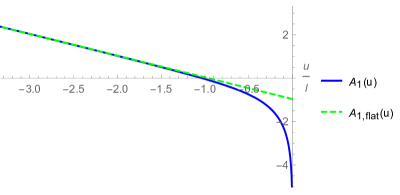
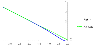
Figure 4: The blue solid lines show the scale factors $A_{1}(u)-A_{1,0}$ (top panel) and $A_{2}(u)-A_{2,0}$ (bottom panel) in the case where the sphere 1 shrinks for $u_{0}/\ell=0$. The constant shifts $A_{1,0}$ is given in equation (5.11), whereas $A_{2,0}$, related to $T_{2,0}$ in (5.11), fixes the initial condition in the IR (see equation (7.2)). It is set so that $T_{2,0}\ell^{2}=20$. The green dashed line represents the same functions, in the case of a flat boundary.

A typical numerical solution for $A_{1,2}(u)$ is presented in Figure 4. The initial conditions are given in the IR: we pick an arbitrary $u_{0}$ then fix $A_{1},\dot{A_{1}}$ and $A_{2}$ at a point $u$ slightly shifted from the IR endpoint ($u=u_{0}-\epsilon$), so that the solution behaves as in (7.2). This fixes all initial conditions of the system (2.19-2.19). While $A_{1}$ and $\dot{A_{1}}$ at the endpoint are fixed by regularity, the value $A_{2,0}$ of $A_{2}$ at $u_{0}-\epsilon$ is free and we vary it to scan over different solutions. For each solution, we then read-off the boundary parameters by analysing the asymptotic behavior as $u\to\infty$, as will be discussed in detailed in subsection 7.1

When $u\to-\infty$, we approach the AdS boundary and the solutions are described by the asymptotic form (4.34) and (4.35). One interesting quantity is the bulk Kretschmann scalar $\mathcal{K}(u)=\ell^{4}R_{ABCD}R^{ABCD}$, whose expression is given by equation (5.2) (with $S=0$ for the CFT case). For the solution corresponding to Figure 4, $\mathcal{K}(u)$ is shown in Figure 5: as expected, as we move towards the interior it deviates from its constant $AdS_{5}$ value (which is attained as $u\to-\infty$). We have verified that the value obtained at $u_{0}$ is in agreement with (5.15).

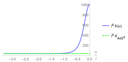
Figure 5: The dimensionless Kretschmann scalar $\ell^{4}\mathcal{K}(u)=\ell^{4}R_{ABCD}R^{ABCD}$ (expressed in terms of the holographic variables in (B.5)) as a function of $u$ for $u_{0}=0$. To be specific we set $T_{2,0}\ell^{2}=20$.

7.1 The UV parameters

Given a numerical solution, we can extract the corresponding values of $\mathcal{R}_{1}$, $\mathcal{R}_{2}$ and $C$ explicitly by fitting the UV region with the asymptotics (4.34) and (4.35).

Let us first clarify the influence of $T_{2,0}\ell^{2}$ on the UV parameters $\mathcal{R}_{2}/\mathcal{R}_{1}$ and $C/\mathcal{R}_{1}^{2}$. Figure 6 shows the evolution of $\mathcal{R}_{2}/\mathcal{R}_{1}$ (recall that this is independent of $u_{0}$) when $T_{2,0}\ell^{2}$ varies from $0$ to $+\infty$. From the figure, we observe the following facts:

• Each choice of $T_{2,0}\ell^{2}$ uniquely fixes the value $\mathcal{R}_{2}/\mathcal{R}_{1}$.

• When the ratio of curvatures is far from unity, increasing $T_{2,0}\ell^{2}$ essentially amounts to increasing the ratio $\mathcal{R}_{2}/\mathcal{R}_{1}$.

• As $T_{2,0}\ell^{2}\to+\infty$, $\mathcal{R}_{2}/\mathcal{R}_{1}\to 1$ in a non-monotonic way: the curvature ratio follows dampened oscillations around the asymptotic value. Thus, there is an infinite number of values of $T_{2,0}\ell^{2}$ for which $\mathcal{R}_{2}/\mathcal{R}_{1}=1$. We shall see later that the dampened oscillations are directly linked to a discrete scaling of the type of an Efimov spiral.

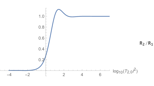
Figure 6: $\frac{\mathcal{R}_{2}}{\mathcal{R}_{1}}(T_{2,0}\ell^{2})$ in the case where the sphere 1 shrinks. The ratio is independent of $u_{0}$.

The other UV parameter $C/\mathcal{R}_{1}^{2}$ follows the same kind of dampened oscillation behavior. Figure 7 gives a complete description of the solutions in the parameter space, that is the plane $\left(\mathcal{R}_{2}/\mathcal{R}_{1},C/\mathcal{R}_{1}^{2}\right)$, both in the case where the sphere 1 shrinks to zero size in the IR and in the symmetric case where the sphere 2 does. The parameter that parametrizes the curve is $T_{2,0}\ell^{2}$ (which increases as one follows the curve from the point $\mathcal{R}_{2}=0$).

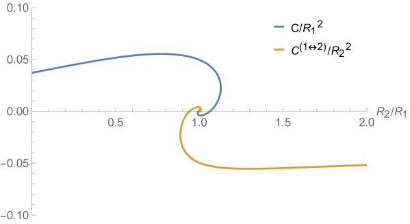
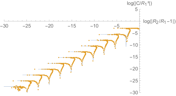
Figure 7: Top: $C/\mathcal{R}_{1}^{2}$ in both the case where the sphere 1 shrinks (blue) and the case where the sphere 2 shrinks (orange). Bottom: The same plot in the case where sphere 1 shrinks, where we represent the logarithm of the distance to the center of the spiral with coordinates $(1,0)$ for each quantity. The orange dots are given by numerical computation while the blue curve is the fit found in (7.19)-(7.20).

Interestingly, we observe that there can be several possible values of $C$ for a given value of the ratio $\mathcal{R}_{2}/\mathcal{R}_{1}$. The resulting figure in the $(\mathcal{R}_{2}/\mathcal{R}_{1},C/\mathcal{R}_{1}^{2})$ plane is a spiral that shrinks exponentially as is apparent from the logarithmic plot in Figure 7. This kind of behavior has been already observed in D-brane models, [27] and holographic V-QCD, [28], and is known as the Efimov spiral.

Remarkably, if both spheres have the same radius in the UV, an infinite number of solutions exist, in which one of the two spheres shrinks but not the other, corresponding to either positive or negative $C$. This translates into a spontaneous breaking of the $\mathbb{Z}^{2}$-symmetry that exchanges the two spheres, which is a symmetry in the UV for ${\mathcal{R}}_{1}={\mathcal{R}}_{2}$. The solution in which the symmetry is unbroken corresponds to the end of the spiral: $C=0$ and $T_{2,0}\to+\infty$. In this case, both spheres shrink, but the solutions is singular in the bulk.

7.2 Efimov spiral

We now investigate the origin of the Efimov spiral, which arises due to the appearance of multiple solutions as the UV radii of the two spheres ${\mathcal{R}_{1}}$ and ${\mathcal{R}_{2}}$ get close to each other.

We follow a reasoning similar to what was done in [28]. The idea is to consider the behavior of a quantity in the bulk theory when its source asymptotes to zero, and look for signs of an instability which will trigger a non-zero vev. Here the relevant source is $\mathcal{R}_{2}-\mathcal{R}_{1}$ and the corresponding quantity $A_{1}-A_{2}$. The latter has the following behavior in the UV, which can be deduced from equations (4.34-4.35):

$$A_{1}(u)-A_{2}(u)\underset{u\to-\infty}{=}\bar{A}_{1}-\bar{A}_{2}+\frac{1}{8}(\mathcal{R}_{2}-\mathcal{R}_{1})e^{2u/\ell}$$ (7.5)

$$+\frac{1}{96}(\mathcal{R}_{1}^{2}-\mathcal{R}_{2}^{2})\,\frac{u}{\ell}\,\mathrm{e}^{4u/\ell}[1+\mathcal{O}(\mathrm{e}^{\Delta_{-}u/\ell})]-\frac{C}{4}e^{4u/\ell}+\mathcal{O}(\mathrm{e}^{6u/\ell})\,.$$

For simplicity we choose $R^{\zeta^{1}}=R^{\zeta^{2}}=2/\ell^{2}$. Note that $C$ is indeed the associated vev (this is how it is defined), which is consistent with the spiral appearing in the plane $(\mathcal{R}_{2}/\mathcal{R}_{1},C/\mathcal{R}_{1}^{2})$.

We now consider the case where:

1. $\mathcal{R}_{1}=\mathcal{R}_{2}$ which is equivalent to $\bar{A}_{1}=\bar{A}_{2}$.

2. $A_{1}-A_{2}$ is infinitesimal, and we define

   $$\epsilon=A_{1}-A_{2}$$ (7.6)

3. We are away from the UV regime, so that

   $$\dot{A}_{1}\simeq 1/(u-u_{0})$$ (7.7)

   (as implied by the asymptotic behavior (7.2), but not too close to the IR end-point $u_{0}$ (where we know that $A_{1}-A_{2}\to-\infty$), so that we can consider $\epsilon$ small.

Condition 1 amounts to choosing $Z_{2}$-symmetric boundary conditions in the UV; in this case, condition 2 certainly holds close to the boundary (by equation (7.5) and condition 1) and down to the point where the radii of the two spheres start deviating due to the non-zero vev $C$. Condition 3 identifies an intermediate region between the UV and the IR, as we explain below.

More precisely, the last condition holds in an intermediate region

$$\alpha_{IR}\ll u_{0}-u\ll\alpha_{UV},\qquad\left\{\begin{array}[]{l}\alpha_{UV}=\ell\\ \alpha_{IR}=\sqrt{\frac{2}{T_{2,0}}}\end{array}\right.\,.$$ (7.8)

In other words, $\alpha_{UV}$ is the UV $AdS$ radius and $\alpha_{IR}$ the IR radius of sphere 2 (see equation (5.12)).

The range (7.8) for the validity of the last condition can be understood as follows. From the asymptotic behavior (7.2), the assumption $A_{1}-A_{2}\ll 1$ is violated in the interior starting from the point $u_{IR}$ where $\log((u_{0}-u_{IR})/\ell)\sim A_{2,0}$, so that (using the relation (5.11)):

$$u_{IR}\approx u_{0}-\ell\mathrm{e}^{A_{2,0}}=u_{0}-\ell\sqrt{R^{\zeta_{2}}/T_{2,0}}$$ (7.9)

is the typical IR boundary of the region satisfying condition 3. Since we are working with $R^{\zeta_{2}}=2/\ell^{2}$, this leads to the identification $\alpha_{IR}$ in equation (7.8).

In the UV, the condition

$$\dot{A}_{1}\sim{1\over(u-u_{0})}$$

is violated starting from the point $u_{UV}$ such that

$$-{1\over\ell}\sim{1\over(u_{UV}-u_{0})}\;,$$

where we used the fact that the leading UV behavior of $A_{1}(u)$ is $A_{1}(u)\sim-{u\over\ell}$. Therefore, in the UV, condition 3 is valid starting approximately at $u_{UV}\approx u_{0}-\ell$. This leads to the upper bound in equation (7.8).

The ratio of the IR length-scale to UV length-scale in (7.8) is then given by:

$${\alpha_{IR}\over\alpha_{UV}}=\sqrt{\frac{2}{T_{2,0}\ell^{2}}}$$ (7.10)

Note that a condition for the validity of our analysis is that $\alpha_{IR}\ll\alpha_{UV}$. This is automatic in the limit $T_{2,0}\to\infty$.

We have checked numerically that in the range (7.8) both conditions 2 and 3 are satisfied: in this range, both (7.6) and (7.7) hold, as shown in figure 8.

\begin{overpic}[width=281.85034pt]{Figures/A1A2vus8_v3} \put(100.0,12.0){$\scriptstyle{\log(u_{0}-u)/\ell}$} \put(85.0,63.0){$\scriptstyle{{A_{1}-A_{2}\over A_{2}}}$} \put(84.0,-3.0){$\alpha_{UV}$} \put(22.0,-3.0){$\alpha_{IR}$} \end{overpic}

\begin{overpic}[width=281.85034pt]{Figures/A1pvus8_v3} \put(100.0,12.0){$\scriptstyle{\log(u_{0}-u)/\ell}$} \put(75.0,63.0){$\scriptstyle{(u-u_{0})A^{\prime}_{1}-1}$} \put(78.0,-3.0){$\alpha_{UV}$} \put(16.0,-3.0){$\alpha_{IR}$} \end{overpic}

Figure 8: These figures show the region of validity of equation (7.13), delimited by the red dashed lines corresponding to the boundary values in equation (7.8). The upper figure is a plot of the relative difference between $A_{1}$ and $A_{2}$, while the lower figure shows the relative difference between $\dot{A}$ and $(u-u_{0})^{-1}$. Both are small in the region delimited by the dashed lines, confirming the validity of equation (7.13) in this regime.

Under the assumptions (7.6) and (7.7), we rewrite the EoM’s (2.19)-(2.21) as an expansion in $\epsilon$. In particular, (2.21) reads, to linear order in $\epsilon$:

$$\ddot{\epsilon}+4\frac{\dot{\epsilon}}{u-u_{0}}(1+\cdots)+T_{1}(\epsilon+\mathcal{O}(\epsilon^{2}))=0,$$ (7.11)

where the dots refer to subleading terms in the expansion in $u-u_{0}$. The quantity $T_{1}$ is given by (4.25) and under the present assumption it reads:

$$T_{1}=4\dot{\epsilon}\dot{A}_{1}-6\ddot{A}_{1}+\mathcal{O}(\ddot{\epsilon})=\frac{6}{(u-u_{0})^{2}}+\cdots+\mathcal{O}(\epsilon)\,.$$ (7.12)

At leading order, the equation for $\epsilon$ is therefore:

$$\ddot{\epsilon}+4\frac{\dot{\epsilon}}{u-u_{0}}+6\frac{\epsilon}{(u-u_{0})^{2}}=0\,,$$ (7.13)

whose solution is given by

$$\epsilon(u)=\left(\frac{u_{0}-u}{\alpha}\right)^{-3/2}\sin\left(\frac{\sqrt{15}}{2}\log\left(\frac{u_{0}-u}{\alpha}\right)+\phi\right)\,,$$ (7.14)

where $\alpha$ and $\phi$ are integration constants. The solution displays two important properties:

• It increases in amplitude as $u_{0}-u\to 0$, which is an expected behavior in the IR. Eventually it diverges, as expected, although this regime lies outside of our linear approximation, and it should only be taken qualitatively.

• It oscillates an infinite number of times close to $u_{0}$. This is at the origin of the Efimov spiral behavior [28].

From the above analysis, we conclude that the singular background with $A_{1}=A_{2}$ all the way to the IR (i.e. $\epsilon(u)\equiv 0$) has a tachyonic instability, signaled by the unbounded growth of the linear perturbation $\epsilon$ in the IR. This instability points to the existence of other solutions where $\epsilon\sim\mathcal{O}(1)$, which have a non-vanishing vev for $A_{1}-A_{2}$. When this parameter is turned on, the system avoids the singular solution.

Now that we have identified the unstable mode at the origin of the spiral, we can keep following the analysis of [28]. The relevant parameter that runs along the spiral is:

$$s=\log\left(\frac{T_{2,0}\ell^{2}}{2}\right)=\log\left(\left(\frac{\alpha_{UV}}{\alpha_{IR}}\right)^{2}\right)$$ (7.15)

which is defined independently of $u_{0}$ as it should. The next step is to connect the UV parameters $(\mathcal{R}_{2}/\mathcal{R}_{1},C/\mathcal{R}_{1}^{2})$ with the IR parameter $T_{2,0}\ell^{2}$. Note that we consider $C/\mathcal{R}_{1}^{2}$ instead of simply $C$ as the former is the $u_{0}$-independent quantity that enters in the free energy (6.17).

To see explicitly how the spiral behavior arises, we need to match solutions (7.14) on both edges of the domain of validity, i.e. for $u_{0}-u\approx\alpha_{UV}$ and $u_{0}-u\approx\alpha_{IR}$.

We first consider the UV regime, we know that $A_{1}-A_{2}$ has a source and a vev term: the former is proportional to $\mathcal{R}_{2}-\mathcal{R}_{1}$, the latter is proportional to $C$ (see equation (7.5)):

$$A_{1}-A_{2}\simeq\bar{A}_{1}-\bar{A}_{2}+\left(\frac{\mathcal{R}_{2}}{\mathcal{R}_{1}}-1\right)e^{2u/\ell}\left(1+\ldots\right)+Ce^{4u/\ell}\left(1+\ldots\right),\qquad u\to-\infty\,,$$ (7.16)

where $\bar{A}_{1}-\bar{A}_{2}=\mathcal{O}\left(\frac{\mathcal{R}_{2}}{\mathcal{R}_{1}}-1\right)$. This regime can be connected to the upper region ($u_{0}-u\approx\alpha_{UV}$) of regime of validity of equation (7.13), where the solution reads:

$$\epsilon_{UV} =K_{R}\;\left(\frac{\mathcal{R}_{2}}{\mathcal{R}_{1}}-1\right)\left(\frac{u_{0}-u}{\alpha_{UV}}\right)^{-3/2}\sin\left(\frac{\sqrt{15}}{2}\ln\left(\frac{u_{0}-u}{\alpha_{UV}}\right)+\phi_{R}\right)$$ (7.17)

$$\hphantom{=}\ +K_{C}\;\frac{C}{\mathcal{R}_{1}^{2}}\left(\frac{u_{0}-u}{\alpha_{UV}}\right)^{-3/2}\sin\left(\frac{\sqrt{15}}{2}\ln\left(\frac{u_{0}-u}{\alpha_{UV}}\right)+\phi_{C}\right)$$

where $K_{R}$, $K_{C}$, $\phi_{R}$ and $\phi_{C}$ are some constants, which are fixed by matching the solution in the UV to (7.16). Note that thus written, this expression for $\epsilon_{UV}$ implies that $\alpha_{UV}$ is the length from which $\dot{\epsilon}$ starts vanishing and should therefore be matched to its UV behavior (7.16). Because it is the same scale as the one for which $\dot{A}_{1}$ should be matched to its UV behavior (which is $\alpha_{UV}$ by definition), the presence of $\alpha_{UV}$ here is justified.

On the other hand, the solution when $u_{0}-u\approx\alpha_{IR}$ reads:

$$\epsilon_{IR}=K_{IR}\;\left(\frac{u_{0}-u}{\alpha_{IR}}\right)^{-3/2}\sin\left(\frac{\sqrt{15}}{2}\ln\left(\frac{u_{0}-u}{\alpha_{IR}}\right)+\phi_{IR}\right),$$ (7.18)

where $K_{IR}$ is another constant. The presence of $\alpha_{IR}$ is justified here by the fact that it is the scale in the IR for which $\epsilon$ should reach $\mathcal{O}(1)$. The two expressions (7.17) and (7.18) are valid in the same region, therefore we can match the coefficients: this gives an expression for $\mathcal{R}_{2}/\mathcal{R}_{1}$ and $C/\mathcal{R}_{1}^{2}$ as functions of $s$ (defined in (7.15)):

$$\frac{\mathcal{R}_{2}}{\mathcal{R}_{1}}-1 = \frac{K_{IR}}{K_{R}}\;\frac{\sin\left(\phi_{IR}-\phi_{C}+\frac{\sqrt{15}}{4}s\right)}{\sin(\phi_{R}-\phi_{C})}\;\mathrm{e}^{-3/4\;s}\,,$$ (7.19)

$$\frac{C}{\mathcal{R}_{1}^{2}} = \frac{K_{IR}}{K_{C}}\;\frac{\sin\left(\phi_{IR}-\phi_{R}+\frac{\sqrt{15}}{4}s\right)}{\sin(\phi_{C}-\phi_{R})}\;\mathrm{e}^{-3/4\;s}\,.$$ (7.20)

These expressions reproduce the spiral behavior: as $s$ increases, the IR radius of the sphere 2 becomes smaller and smaller, and it reaches zero in the singular limit ($s\to\infty)$. At the same time, the vev parameter $C$ decreases and the UV ratio ${\mathcal{R}}_{2}/{\mathcal{R}}_{1}$ oscillates, crossing unity an infinite number of times. Therefore, if we consider the symmetric UV boundary condition ${\mathcal{R}}_{2}/{\mathcal{R}}_{1}=1$, we find an infinite number of solutions, for the values of $s$ which correspond to the vanishing of the $sin$ function in the numerator of equation (7.19) .

Note that because the spiral turns clockwise, $C/\mathcal{R}_{1}^{2}$ is ahead of $\mathcal{R}_{2}/\mathcal{R}_{1}-1$, which means that $\sin(\phi_{R}-\phi_{C})<0$.
The fit corresponding to those solutions is plotted in Figure 7.

7.3 The dominant vacuum

The degeneracy which originates from the Efimov spiral close to the singular point indicates that for a boundary CFT characterized by a given value of the ratio $\mathcal{R}_{2}/\mathcal{R}_{1}$, there are several possible values for the vev $C$, that is, several possible vacuum states (saddle points). The number of possible vacua increases when the ratio tends to 1, asymptoting to infinity for $\mathcal{R}_{2}=\mathcal{R}_{1}$. For each fixed value of $\mathcal{R}_{2}/\mathcal{R}_{1}$ the dominant vacuum is the one with the lowest free energy (on-shell action).

Numerical evaluation of the free energy of the solution using equation (6.21) shows that the dominant vacuum is the first one reached (for a given $\mathcal{R}_{2}/\mathcal{R}_{1}$) when moving towards the center of the spiral. This is displayed in Figure 9, which shows the finite part of the free energy (i.e. the term $\overline{\mathcal{F}}$ in equation (6.13)) as a function of $\mathcal{R}_{2}/\mathcal{R}_{1}$. As a result, the Efimov degeneracy is broken and there is only one possible vacuum for every value of $\mathcal{R}_{2}/\mathcal{R}_{1}$, except at the critical point $\mathcal{R}_{2}=\mathcal{R}_{1}$ where both $C$ and $-C$ are possible, corresponding to the spontaneous breaking of the $\mathbb{Z}^{2}$-symmetry that exchanges the two spheres. The system therefore exhibits a bifurcation at this point, where the vev $C$ changes sign and the sphere that shrinks in the IR is exchanged.

\begin{overpic}[width=281.85034pt]{Figures/FUvR_sym_u} \put(104.0,56.0){${\mathcal{R}_{2}\over\mathcal{R}_{1}}$} \put(4.0,58.0){$\bar{\mathcal{F}}$} \end{overpic}

Figure 9: Finite part $\bar{\mathcal{F}}$ of the the free energy (E.43) as a function of the ratio $\mathcal{R}_{2}/\mathcal{R}_{1}$, in both the case where the sphere 1 shrinks (blue) and the case where the sphere 2 shrinks (orange). We normalize by the overall volume factor $32\pi^{2}M_{p}^{3}\ell^{3}$. The point where the two curves first cross at $\mathcal{R}_{1}=\mathcal{R}_{2}$ corresponds to a bifurcation, where the sphere that shrinks is exchanged and the vev changes sign.

Another point that deserves attention is the behavior of the radius of the sphere that does not shrink to zero size in the IR (the sphere 2 here). To be more specific, we computed numerically the radius of the non-vanishing sphere at the endpoint, given in equation (5.12), as a function of $R_{2}/R_{1}$. The result is displayed in figure 10.

\begin{overpic}[scale={0.80}]{Figures/aIRvR} \put(101.0,4.0){${\mathcal{R}_{2}\over\mathcal{R}_{1}}$} \put(-2.0,66.0){$\alpha_{IR}/\ell$} \end{overpic}

Figure 10: The IR endpoint radius $\alpha_{IR}$ of the sphere which stays finite at the end-point of the flow, as a function of the curvature ratio $\mathcal{R}_{2}/\mathcal{R}_{1}$. The blue curve corresponds to $\alpha^{IR}_{2}$ in the case where sphere 1 shrinks to zero size in the IR; the yellow curve to $\alpha^{IR}_{1}$ in the solution where the sphere 2 shrinks to zero. The transition which exchanges the two spheres corresponds to the point where the curves cross at the largest value for the radius.

8 Holographic RG-flows on S${}^{2}\times$ S²

We now move to consider RG-flow geometries, where the scalar field is not constant. They originate in the UV from a maximum of the potential (at $\varphi=0$) and end regularly when one of the spheres shrinks to zero size. At this point, the scalar reaches a value $\varphi=\varphi_{0}$ which lies in the region between this maximum and (typically) the nearest minimum.

We consider solutions where $\varphi$ changes monotonically along the flow from UV to IR. Therefore one can use $\varphi$ as a coordinate along the flow. We still assume that sphere 1 shrinks in the IR (i.e. $A_{1}(\varphi)\xrightarrow[\varphi\to\varphi_{0}]{}-\infty$ which implies that $A_{2}$ remains finite to have regularity in the interior according to B).

These solutions are generic, as they arise for generic potentials as long as they possess at least one maximum and one minimum. The simplest such potential is the following quadratic-quartic function:

$$V(\varphi)=-\frac{12}{\ell^{2}}-\frac{m^{2}}{2}\varphi^{2}+\lambda\varphi^{4}$$ (8.1)

This potential has one maximum at $\varphi_{max}=0$. For purposes of illustration we choose $\lambda=m^{2}/4$ so that the minima occur at $\varphi_{min}=\pm 1$. The qualitative features of the solutions do not depend on this choice.

We then proceed by solving (3.3)-(3.6) numerically for $W_{1}(\varphi),W_{2}(\varphi)$ and $S(\varphi)$. Like in the case with no scalar field, to impose regularity we specify boundary conditions for $W_{1},W_{2}$ and $S$ at the IR end point $\varphi_{0}$, as prescribed by equations (5.3-5.7), with $T_{2,0}$ as a free parameter. Given the symmetry of the setup, we restrict our attention to flows that end in the region $\varphi_{0}\in[0,1]$.

8.1 General properties of the RG flow

We first discuss general properties of the flow solution of the equations of motion (2.12)-(2.15) obtained numerically. The IR parameters one can vary are $\varphi_{0}$ and $T_{2,0}\ell^{2}$. These determine all other terms in the IR expansion, as well as all the dimensionless UV data. More specifically, in the vicinity of the UV fixed point the solutions are described by the family of solutions collectively denoted by $W_{1}^{-}$ and $W_{2}^{-}$ in section 4. These solutions depend on the four independent dimensionless parameters $\mathcal{R}_{1}$, $\mathcal{R}_{2}$, $C_{1}$ and $C_{2}$. There is one more parameter than in the CFT case (where $C_{1}+C_{2}=0$), corresponding to the fact that the vev of the scalar operator is now a free parameter of the UV theory.

Below, we analyze separately the dependence on each of the two IR parameters $\varphi_{0}$ and $T_{2,0}\ell^{2}$.

Fixed $T_{2,0}\ell^{2}$

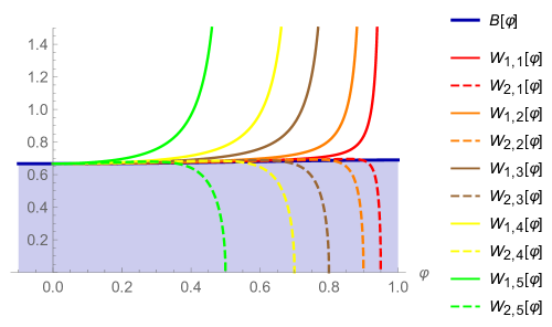
Figure 11: Solutions $W_{1}(\varphi)$ and $W_{2}(\varphi)$ for the potential (8.1) with $\Delta_{-}=1.2$ in the case where the sphere 1 shrinks. The five solutions $(W_{1,i},W_{2,i})$ with $i=1,\dots,5$ differ in the value of their IR endpoint $\varphi_{0}$ for $T_{2,0}\ell^{2}=4.5$. The critical curve is defined as $B(\varphi)\equiv\sqrt{-V(\varphi)/3}$. In the case of $S^{4}$ [17], the superpotential $W(\varphi)$ cannot enter the area below the critical curve, which is depicted as the shaded region.

In Figure 11 we exhibit solutions for the superpotentials $W_{1}(\varphi)$ and $W_{2}(\varphi)$ corresponding to generic RG flows for a bulk potential given by (8.1) with $T_{2,0}\ell^{2}$ fixed, and for different values of the endpoint $\varphi_{0}$. To be specific, we have set $\Delta_{-}=1.2$ and $T_{2,0}\ell^{2}=4.5$ but our observations hold more generally.

• The main result is that for every value of $\varphi_{0}$ between $\varphi_{max}=0$ and $\varphi_{min}=1$ there exists a unique solution to the superpotential equations (3.3)-(3.6) (remember that $T_{2,0}\ell^{2}$ has been fixed) corresponding to an RG flow originating from the UV fixed point at $\varphi_{max}=0$ and ending at $\varphi_{0}$.

• Note that whereas $W_{1}(\varphi)$ diverges like $(\varphi_{0}-\varphi)^{-1/2}$ when approaching the IR end point $\varphi_{0}$, $W_{2}(\varphi)\to 0$. This is in agreement with the analytical results found in Section 5.

• The counting of parameters is as expected: picking a solution with the regular IR behavior for a RG flow fixes two combinations of the four UV parameters; the remaining freedom is then equivalent to the choice of IR end point $\varphi_{0}$, together with the choice of the radius in the interior of the sphere that does not shrink at $\varphi_{0}$ (here the sphere 2), which is given by $T_{2,0}$. Therefore, regularity plus a choice of $\varphi_{0}$, $T_{2,0}$ uniquely determines the solution.

• The solution is then matched to the UV asymptotics (4-4) to extract the UV quantities ${\mathcal{R}}_{1,2}$ and $C_{1,2}$. The two IR parameters $\varphi_{0},T_{2,0}$ can then be traded for the two independent UV parameters ${\mathcal{R}}_{1,2}$, and the vev parameters $C_{1,2}$ can then be expressed as functions of ${\mathcal{R}}_{1,2}$.

Fixed $\varphi_{0}$

We now keep $\varphi_{0}$ fixed and let $T_{2,0}$ vary. In Figure 12 we exhibit solutions for the superpotentials $W_{1}(\varphi)$ and $W_{2}(\varphi)$ corresponding to generic RG flows for a bulk potential given by (8.1) when $\varphi_{0}$ is fixed. To be specific we have set $\Delta_{-}=1.2$ and $\varphi_{0}=0.8$ but our observations hold more generally.

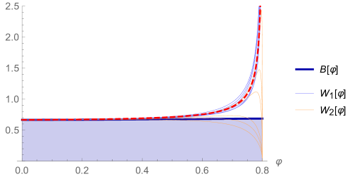
Figure 12: Solutions $W_{1}(\varphi)$ and $W_{2}(\varphi)$ for the potential (8.1) with $\Delta_{-}=1.2$ in the case where the sphere 1 shrinks. The six solutions differ in the value of $T_{2,0}$ whereas $\varphi_{0}=0.8$ is fixed. From the lowest curve for $W_{2}$ to the highest one, $T_{2,0}\ell^{2}$ increases, taking successively the values: $0.9,4.5,13,5,90,270$. The red dashed curve is the one towards which $W_{2}$ tends when $T_{2,0}\ell^{2}\to+\infty$ on every interval in $[0,\varphi_{0}[$. The critical curve is defined as $B(\varphi)\equiv\sqrt{-V(\varphi)/3}$. In the case of $S^{4}$ [17], the superpotential $W(\varphi)$ cannot enter the area below the critical curve, which is depicted as the shaded region.

• Because $\varphi_{0}$ is fixed, there is a unique solution for every $T_{2,0}\ell^{2}$.

• As $T_{2,0}$ grows, $W_{2}$ goes to a value ever higher in the interior before diving to 0 to have regularity. More precisely we observe that both $W_{1}$ and $W_{2}$ approach a single curve (the red-dashed curve in Figure 12) as $T_{2,0}\ell^{2}\to\infty$. This curve corresponds to the singular solution, where both $W_{1}$ and $W_{2}$ diverge in the IR and both spheres shrink to zero size.

UV parameters.

Given a numerical solution, we can extract the corresponding values of $\mathcal{R}_{1}$, $\mathcal{R}_{2}$, $C_{1}$ and $C_{2}$ explicitly by fitting the UV region with the asymptotics (4)-(4). Figure 13 represents $\mathcal{R}_{1}$ and $C_{1}-C_{2}$ as functions of $\varphi_{0}$ when $T_{2,0}=0$. In this section, $C_{1}-C_{2}$ is defined as the full vev term for $A_{1}-A_{2}$, which corresponds to make the following redefinition in equation (4.16)

$$C_{1}\to C_{1}+\frac{\mathcal{R}_{1}^{2}-\mathcal{R}_{2}^{2}}{24\Delta_{-}}\log(|\varphi_{-}|\ell^{\Delta_{-}}),\quad C_{2}\to C_{2}-\frac{\mathcal{R}_{1}^{2}-\mathcal{R}_{2}^{2}}{24\Delta_{-}}\log(|\varphi_{-}|\ell^{\Delta_{-}}).$$ (8.2)

This redefinition does not affect $C_{1}+C_{2}$.

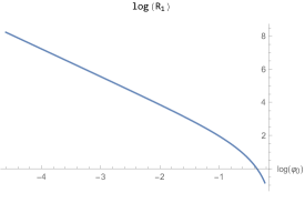
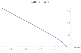
Figure 13: $\mathcal{R}_{1}(\varphi_{0})$ and $C_{1}(\varphi_{0})-C_{2}(\varphi_{0})$ in the case where the sphere 1 shrinks and for $T_{2,0}=0$. In this situation the space 2 is flat ($\mathcal{R}_{2}=0$).

We observe that for small $\varphi_{0}$, $\mathcal{R}_{1}\propto\varphi_{0}^{-2/\Delta_{-}}$ and $C_{1}-C_{2}\propto\varphi_{0}^{-4/\Delta_{-}}$. These properties can once again be deduced from the scaling properties of the equations of motion (3.3) - (3.6) under a shift of $u\to u+\delta u$: under such shift, in the UV we have: Indeed, $\varphi(u)\sim\varphi_{-}\ell^{\Delta_{-}}\mathrm{e}^{\Delta_{-}(\delta u/\ell)}$ in the UV. This implies that, if $u_{0}$ is the IR coordinate of the endpoint, then

$$\varphi_{0}\propto\varphi_{-}\ell^{\Delta_{-}}\mathrm{e}^{\Delta_{-}u_{0}/\ell}$$ (8.3)

The above equation gives either the dependence of $\varphi_{-}$ on $u_{0}$ when $\varphi_{0}$ is fixed, or the dependence of $\varphi_{0}$ when $\varphi_{-}$ is fixed. It is apparent from $\varphi_{0}\xrightarrow[u_{0}\to+\infty]{}1$ that (8.3) is only valid for $\varphi_{0}\ll 1$.

The scalings of the UV parameters in terms of $\varphi_{0}$ when $\varphi_{0}\ll 1$ can then be deduced from the scaling properties of the EoMs (2.12)-(2.15) under the translation $u\to u-u_{0}$. In particular, under such a translation, the leading terms in the near boundary expansion (4)-(4) should have the same scaling. It implies in particular that the terms at order 1 in curvature in the expansion of $W_{1}$ and $W_{2}$ should be invariant under such a translation, which gives the expected scaling in $\varphi_{0}$ for $\mathcal{R}_{1}$ and $\mathcal{R}_{2}$ when $\varphi_{0}\ll 1$ (in which case (8.3) can be used to relate $\varphi_{0}$ with $u_{0}$). Knowing this, the expansion of $W_{1}-W_{2}$ gives the appropriate scaling for $C_{1}-C_{2}$, and that of $S$ (4) gives the $\varphi_{0}$-dependence for the scalar vev $C_{1}+C_{2}$ (which is not the same as $C_{1}-C_{2}$):

$$C_{1}+C_{2}\propto\varphi_{0}^{\frac{\Delta_{-}-\Delta_{+}}{\Delta_{-}}}\;\;\;,\;\;\;\varphi_{0}\ll 1$$ (8.4)

Figure 14 represents $C_{1}+C_{2}$ as a function of $\varphi_{0}$ when $T_{2,0}=0$.

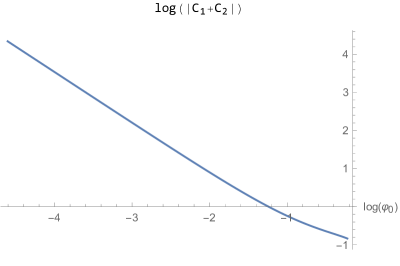
Figure 14: $C_{1}(\varphi_{0})+C_{2}(\varphi_{0})$ in the case where the sphere 1 shrinks and for $T_{2,0}=0$. In this situation the space 2 is flat ($\mathcal{R}_{2}=0$).

Note that whereas $\mathcal{R}_{1}$, $\mathcal{R}_{2}$ and $C_{1}-C_{2}$ tend to 0 when $\varphi_{0}\to 1$ (flat limit), the scalar vev tends to a finite value. This is again coherent with what was found in the $S^{4}$ case [17].

8.2 Efimov spiral and dominant vacuum

As in the conformal case, in the $Z_{2}$ symmetric limit ${\mathcal{R}}_{2}/{\mathcal{R}}_{1}\to 1$ we encounter again a discrete Efimov scaling and an infinite number of solutions.

Figure 15 shows the Efimov spiral in the plane $(\mathcal{R}_{2}/\mathcal{R}_{1},(C_{1}-C_{2})/\mathcal{R}_{1}^{2})$. The behavior is essentially the same as what was observed without a scalar field, with the notable property that the amplitudes $(K_{C},K_{R})$ and the phases $(\varphi_{C},\varphi_{R})$ defined in equations (7.19) and (7.20) are now functions of $\varphi_{0}$: there is a continuous family of spirals parametrized by $\varphi_{0}$.

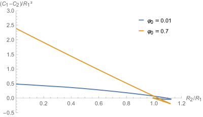
Figure 15: The Efimov spiral in the plane $(\mathcal{R}_{2}/\mathcal{R}_{1},(C_{1}-C_{2})/\mathcal{R}_{1}^{2})$, in the case where the sphere 1 shrinks and for $\varphi_{0}=0.01$ and $\varphi_{0}=0.7$. Although it is difficult to see a “spiral” in the plot above, it can be inferred as it is similar to the one plotted on the top of figure 16. For values of $\varphi_{0}$ intermediate between $0.01$ and $0.8$, there is a continuous family of spirals that fills the space between the two spirals that are plotted.

Figure 16 shows the spiral for the a fixed endpoint value, $\varphi_{0}=0.1$.

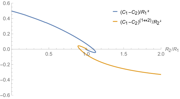
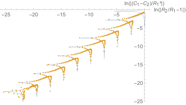
Figure 16: Top: $(C_{1}-C_{2})/\mathcal{R}_{1}^{2}$ in both the case where the sphere 1 shrinks (blue) and the case where the sphere 2 shrinks (orange) and for $\varphi_{0}=0.1$. Bottom: The same plot in the case where 1 shrinks, where we represent the logarithm of the distance to the center of the spiral with coordinates $(1,0)$ for each quantity. The orange dots are given by numerical computation while the blue curve is the fit found in (7.19)-(7.20).

With a scalar field, the equation for $\epsilon\equiv A_{1}-A_{2}$ (7.13) (given the same conditions) at leading order is the same:

$$\ddot{\epsilon}+4\frac{\dot{\epsilon}}{u-u_{0}}+6\frac{\epsilon}{(u-u_{0})^{2}}=0$$ (8.5)

The formulae that describe the spiral (7.19)-(7.20) are therefore exactly the same as without a scalar field, where the amplitudes $(K_{C},K_{R})$ and the phases $(\varphi_{C},\varphi_{R})$ are functions of $\varphi_{0}$.

We use equation (6.12) to compare the free energy of two vacua with the same ratio $\mathcal{R}_{2}/\mathcal{R}_{1}$ and value of $\varphi_{0}$, but with distinct vevs $(C_{1}-C_{2})/\mathcal{R}_{1}^{2}$. The conclusion is the same as the one reached in section 7 without the scalar field: the stable vacuum corresponds to the first point that is reached by the spiral in the $(\mathcal{R}_{2}/\mathcal{R}_{1},(C_{1}-C_{2})/\mathcal{R}_{1}^{2})$-plane. There is therefore a bifurcation at the point $\mathcal{R}_{1}=\mathcal{R}_{2}$, where the sphere that shrinks is exchanged and $C_{1}-C_{2}$ changes sign.

\begin{overpic}[width=281.85034pt]{Figures/FUvR_sym_f} \put(104.0,4.0){${\mathcal{R}_{2}\over\mathcal{R}_{1}}$} \put(4.0,63.0){$\bar{\mathcal{F}}$} \end{overpic}

Figure 17: Finite part $\bar{\mathcal{F}}$ of the the free energy (E.43) as a function of the ratio $\mathcal{R}_{2}/\mathcal{R}_{1}$, on the line of the $(\mathcal{R}_{1},\mathcal{R}_{2})-$plane where the radius of the sphere which shrinks to zero size in the IR is kept fixed. We represent both the case where the sphere 1 shrinks (blue) and the case where the sphere 2 shrinks (orange). We normalize by the overall volume factor $32\pi^{2}M_{p}^{3}\ell^{3}$. The point where the two curves first cross at $\mathcal{R}_{1}=\mathcal{R}_{2}$ corresponds to a bifurcation, where the sphere that shrinks is exchanged and the asymmetric vev changes sign.

Appendix

Appendix A Matching to known cases

In this appendix we show that the general equations (2.7)-(2.10) match known special cases.

1. When all $d_{k}=1$ and $A_{i}=A_{j}=A$, this is the same as the flat slice case. We do recover the equations of motion for the flat slicing ansatz:

   $$2(d-1)\ddot{A}+\dot{\varphi}^{2} =0\,,$$ (A.1)

   $$d(d-1)\dot{A}^{2}-\frac{1}{2}\dot{\varphi}^{2}+V =0\,,$$ (A.2)

   $$\ddot{\varphi}+d\dot{A}\dot{\varphi}-V^{\prime} =0\,.$$ (A.3)

2. When all $d_{k}=1$, and $A_{1}$ is distinct from all others $A_{j\not=1}$ which are equal, the metric is

   $$ds^{2}=du^{2}+e^{2A_{1}}dt^{2}+e^{2A_{2}}d\vec{x}^{2}$$ (A.4)

   By a change of coordinates, the metric can be put in the black hole form

   $$ds^{2}={d\tilde{u}^{2}\over f}+e^{2A}(fdt^{2}+d\vec{x}^{2})$$ (A.5)

   We have

   $$A=A_{2}\;\;\;,\;\;\;f=e^{2(A_{1}-A_{2})}\;\;\;,\;\;\;d\tilde{u}=e^{A_{1}-A_{2}}du$$ (A.6)

   The equations for ((A.5)) are

   $$2(d-1)\ddot{A}(u)+\dot{\varphi}^{2}(u)=0,$$ (A.7)

   $$\ddot{f}(u)+d\dot{f}(u)\dot{A}(u)=0\Rightarrow\dot{f}=C~{}e^{-dA}$$ (A.8)

   $$(d-1)\dot{A}(u)\dot{f}(u)+f(u)\left[d(d-1)\dot{A}^{2}(u)-\frac{\dot{\varphi}^{2}}{2}\right]+V(\phi)=0.$$ (A.9)

   $$\ddot{\varphi}(u)+\left(d\dot{A}(u)+{\dot{f}(u)\over f(u)}\right)\dot{\varphi}(u)-{V^{\prime}\over f(u)}=0$$ (A.10)

   From ((2.7))-((2.10)) with $d_{k}=1$, $A_{1}\neq A_{j}$ with $j=2,\ldots,d$ we obtain the following equations

   $$\ddot{A}_{2}-\dot{A}_{2}\left(\dot{A}_{1}-\dot{A}_{2}\right)+\frac{\dot{\varphi}^{2}}{2(d-1)}=0,$$ (A.11)

   $$2((d-2)\ddot{A}_{2}-\dot{A}_{1}\dot{A}_{2}+\ddot{A}_{1}+\dot{A}^{2}_{1})+\dot{\varphi}^{2}=0,$$ (A.12)

   $$2(d-1)\dot{A}_{1}\dot{A}_{2}+(d-1)(d-2)\dot{A}^{2}_{2}-\frac{1}{2}\dot{\varphi}^{2}+V=0,$$ (A.13)

   $$\ddot{\varphi}+\dot{A}_{1}\dot{\varphi}+(d-1)\dot{A}_{2}\dot{\varphi}-V^{\prime}=0.$$ (A.14)

   Implementing the redefinitions in ((A.6)) and converting to derivatives with respect to $\tilde{u}$, we obtain eqs. ((A.7))-((A.10)).

3. When $d_{k}=d$ we have a single scale factor and this is case analyzed in [17]. The equations match with those derived there.

4. When $d_{1}=1$ and $d_{2}=d-1$ we have the $S^{1}\times S^{d-1}$ slice. The solution with constant potential should be global AdS_d+1.
   For this case we have the following equations of motion

   $$(d-1)(d-2)\dot{A}^{2}_{2}+2(d-1)\dot{A}_{1}\dot{A}_{2}-e^{-2A_{2}}R^{\zeta^{2}}-\frac{1}{2}\dot{\varphi}^{2}+V=0,$$ (A.15)

   $$2(d-1)\left(\ddot{A}_{2}-\dot{A}_{2}\left(\dot{A}_{1}-\dot{A}_{2}\right)\right)+\dot{\varphi}^{2}=0,$$ (A.16)

   $$2(\ddot{A}_{1}+(d-2)\ddot{A}_{2}+\dot{A}_{1}(\dot{A}_{1}-\dot{A}_{2})+\frac{1}{d-1}e^{-2A_{2}}R^{\zeta^{2}})+\dot{\varphi}^{2}=0,$$ (A.17)

   $$\ddot{\varphi}+\dot{A}_{1}\dot{\varphi}+(d-1)\dot{A}_{2}\dot{\phi}-V^{\prime}=0,$$ (A.18)

   which with $V=-{d(d-1)\over\ell^{2}}$ and $R^{\zeta^{2}}={(d-1)(d-2)\over R^{2}}$ can be reduced to the form

   $$\dot{A}_{2}((d-2)\dot{A}_{2}+2\dot{A}_{1})-e^{-2A_{2}}{(d-2)\over R^{2}}-{d\over\ell^{2}}=0,$$ (A.19)

   $$\ddot{A}_{2}-\dot{A}_{2}\left(\dot{A}_{1}-\dot{A}_{2}\right)=0,$$ (A.20)

   $$\ddot{A}_{1}+(d-2)\ddot{A}_{2}+\dot{A}_{1}(\dot{A}_{1}-\dot{A}_{2})+e^{-2A_{2}}{(d-2)\over R^{2}}=0.$$ (A.21)

   The solution to the above equations is indeed AdS space in global coordinates

   $$e^{2A_{1}}=C_{1}^{2}\cosh^{2}\left({u\over\ell}\right)\;\;\;,\;\;\;e^{2A_{1}}={\ell^{2}\over R^{2}}\sinh^{2}\left({u\over\ell}\right)$$ (A.22)

Appendix B The curvature invariants

In this appendix we shall compute the curvature scalars, $R$, $R_{AB}R^{AB}$ and $R_{ABCD}R^{ABCD}$ and we shall express them in terms of the first order functions $W_{1}$, $W_{2}$, $S$, $T_{1}$ and $T_{2}$.

The Ricci scalar

The Ricci scalar is found to be

$$R=-(4\ddot{A_{1}}+4\ddot{A_{2}}+6\dot{A_{1}}^{2}+6\dot{A_{2}}^{2}+8\dot{A_{1}}\dot{A_{2}})+R^{\zeta_{1}}\mathrm{e}^{-2A_{1}}+R^{\zeta_{2}}\mathrm{e}^{-2A_{2}}.$$ (B.1)

Using the equations of motion, this can be written as

$$R=\frac{S^{2}}{2}+\frac{5}{3}V.$$ (B.2)

As $V$ is regular everywhere for finite $\varphi$, regularity of the scalar curvature is guaranteed once $\dot{\phi}$ is regular.

Ricci squared

The square of the Ricci tensor is given by

$$R_{AB}R^{AB}=4(\ddot{A_{1}}+\ddot{A_{2}}+\dot{A_{1}}^{2}+\dot{A_{2}}^{2})^{2}+16\dot{A_{1}}^{2}\dot{A_{2}}^{2}$$ (B.3)

$$\mathrel{\phantom{=}}{}+8\dot{A_{1}}\dot{A_{2}}(\ddot{A_{1}}+2\dot{A_{1}}^{2}-{R^{\zeta_{1}}\over 2}\mathrm{e}^{-2A_{1}}+\ddot{A_{2}}+2\dot{A_{2}}^{2}-{R^{\zeta_{2}}\over 2}\mathrm{e}^{-2A_{2}})$$

$$\mathrel{\phantom{=}}{}+2(\ddot{A_{1}}+2\dot{A_{1}}^{2}-{R^{\zeta_{1}}\over 2}\mathrm{e}^{-2A_{1}})^{2}+2(\ddot{A_{2}}+2\dot{A_{2}}^{2}-{R^{\zeta_{2}}\over 2}\mathrm{e}^{-2A_{2}})^{2}.$$

Using the equations of motion, this can be written as

$$R_{AB}R^{AB}=\left(\frac{S^{2}}{2}+\frac{V}{3}\right)^{2}+\frac{4V^{2}}{9}$$ (B.4)

The regularity conditions are as in the case of scalar curvature.

Riemann squared

The Kretschmann scalar reads

$$R_{ABCD}R^{ABCD}=(R^{\zeta_{1}})^{2}\mathrm{e}^{-4A_{1}}+(R^{\zeta_{2}})^{2}\mathrm{e}^{-4A_{2}}+12\dot{A_{1}}^{4}+12\dot{A_{2}}^{4}+8\ddot{A_{1}}^{2}+8\ddot{A_{2}}^{2}$$ (B.5)

$$\mathrel{\phantom{=}}{}+8\dot{A_{1}}^{2}(2\ddot{A_{1}}-{R^{\zeta_{1}}\over 2}\mathrm{e}^{-2A_{1}})+8\dot{A_{2}}^{2}(2\ddot{A_{2}}-{R^{\zeta_{2}}\over 2}\mathrm{e}^{-2A_{2}})+16\dot{A_{1}}^{2}\dot{A_{2}}^{2}.$$

In general, we can rewrite the expression as

$$R_{ABCD}R^{ABCD}=8(\ddot{A_{1}}+\dot{A_{1}}^{2})^{2}+8(\ddot{A_{2}}+\dot{A_{2}}^{2})^{2}+16\dot{A_{1}}^{2}\dot{A_{2}}^{2}$$ (B.6)

$$\mathrel{\phantom{=}}{}+(R^{\zeta_{1}})^{2}\mathrm{e}^{-4A_{1}}+4\dot{A_{1}}^{4}-4R^{\zeta_{1}}\dot{A_{1}}^{2}\mathrm{e}^{-2A_{1}}+(R^{\zeta_{2}})^{2}\mathrm{e}^{-4A_{2}}+4\dot{A_{2}}^{4}-4R^{\zeta_{2}}\dot{A_{2}}^{2}\mathrm{e}^{-2A_{2}}$$

$$=4(\ddot{A_{1}}+\dot{A_{1}}^{2}+\ddot{A_{2}}+\dot{A_{2}}^{2})^{2}+4(\ddot{A_{1}}+\dot{A_{1}}^{2}-\ddot{A_{2}}-\dot{A_{2}}^{2})^{2}+16\dot{A_{1}}^{2}\dot{A_{2}}^{2}$$

$$\mathrel{\phantom{=}}{}+4(\dot{A_{1}}^{2}-{R^{\zeta_{1}}\over 2}\mathrm{e}^{-2A_{1}})^{2}+4(\dot{A_{2}}^{2}-{R^{\zeta_{2}}\over 2}\mathrm{e}^{-2A_{2}})^{2}.$$

We also have

$$4(\ddot{A_{1}}+\dot{A_{1}}^{2}+\ddot{A_{2}}+\dot{A_{2}}^{2})^{2}=\left({S^{2}\over 2}+{1\over 3}V\right)^{2}$$ (B.7)

$$4(\ddot{A_{1}}+\dot{A_{1}}^{2}-\ddot{A_{2}}-\dot{A_{2}}^{2})^{2}=\left(S(W_{1}^{\prime}-W_{2}^{\prime})-{W_{1}^{2}-W_{2}^{2}\over 2}\right)^{2}$$ (B.8)

$$4(\dot{A_{1}}^{2}-{R^{\zeta_{1}}\over 2}\mathrm{e}^{-2A_{1}})^{2}=\left({W_{1}^{2}\over 2}-T_{1}\right)^{2}=\left({W_{1}^{2}\over 2}+S^{2}+W_{2}^{2}-W_{1}W_{2}-S(W_{1}^{\prime}+W_{2}^{\prime})\right)^{2}$$ (B.9)

$$4(\dot{A_{2}}^{2}-{R^{\zeta_{2}}\over 2}\mathrm{e}^{-2A_{2}})^{2}=\left({W_{2}^{2}\over 2}-T_{2}\right)^{2}=\left({W_{2}^{2}\over 2}+S^{2}+W_{1}^{2}-W_{1}W_{2}-S(W_{1}^{\prime}+W_{2}^{\prime})\right)^{2}$$ (B.10)

Therefore we can convert

$$R_{ABCD}R^{ABCD}=\left(\frac{S^{2}}{2}+\frac{V}{3}\right)^{2}+\left(S(W_{1}^{\prime}-W_{2}^{\prime})-{W_{1}^{2}-W_{2}^{2}\over 2}\right)^{2}+W_{1}^{2}W_{2}^{2}$$ (B.11)

$$+\left({W_{1}^{2}\over 2}+S^{2}+W_{2}^{2}-W_{1}W_{2}-S(W_{1}^{\prime}+W_{2}^{\prime})\right)^{2}+\left({W_{2}^{2}\over 2}+S^{2}+W_{1}^{2}-W_{1}W_{2}-S(W_{1}^{\prime}+W_{2}^{\prime})\right)^{2}$$

It is useful to rewrite this equation in terms of $A_{1}$ and $A_{2}$:

$$R_{ABCD}R^{ABCD}=\frac{11}{2}\left(\frac{S^{2}}{2}+\frac{V}{3}\right)^{2}-2S^{2}V-S^{4}$$

$$+\,\,6(\ddot{A_{1}}+\dot{A_{1}}^{2}-\ddot{A_{2}}-\dot{A_{2}}^{2})^{2}+48(\dot{A_{1}}\dot{A_{2}})^{2}+8V\dot{A_{1}}\dot{A_{2}}-4S^{2}\dot{A_{1}}\dot{A_{2}}$$ (B.12)

When $A_{1}=A_{2}$, this expression reduces to

$$R_{ABCD}R^{ABCD}=8\mathrm{e}^{-4A}+40\dot{A}^{4}-16\dot{A}^{2}\mathrm{e}^{-2A}+16\ddot{A}^{2}+32\dot{A}^{2}\ddot{A}$$ (B.13)

$$=\left(\frac{S^{2}}{2}+\frac{V}{3}\right)^{2}+\frac{1}{24}(S^{2}-2V)^{2}+\frac{1}{3}T^{2},$$

where $T=T_{1}+T_{2}=4\exp(-2A)$. In this case it is singular when $T\to\infty$.

Appendix C The regularity conditions on the interior geometry

We study here the regularity of the solutions near end-points of the flow where $S\to 0$. As a guiding criterion for regularity we use the finiteness of the Kretschmann scalar, whose expression was derived in the previous appendix, equation (B). As we shall see, this will turn out to be a sufficient (not just necessary) condition to identify regular geometries.

C.1 Analysis of the IR behavior of solutions

C.1.1 Leading behavior

Regular flows stop at a point $u_{0}$ where $\dot{\varphi}(u_{0})=0$. We want to understand the behavior of the scale factors near such a point.

We start by assuming a generic power-law leading behavior near $u_{0}$ of the form: $A_{1}(u)$ and $A_{2}(u)$ is

$$A_{1}=\lambda_{1}(u_{0}-u)^{a}+\ldots\;\;\;,\;\;\;A_{2}=\lambda_{2}(u_{0}-u)^{b}+\ldots\,\quad u\to u_{0}$$ (C.1)

where $\lambda_{1}$,$a$ and $\lambda_{2}$,$b$ are constants such that $a\leq 0$, $b\leq 0$ and $\lambda_{1},\lambda_{2}\neq 0$. We further assume the following ansatz for $\dot{\varphi}(u)$ near $u_{0}$:

$$\dot{\varphi}=C_{0}(u_{0}-u)^{c}+\cdots\;\;\;,\;\;\;u\to u_{0}\;\;\;,\;\;\;c>0\;\;\;,\;\;\;C_{0}\neq 0.$$ (C.2)

Substituting the asymptotics (C.1) and (C.2) into equations (3.7) and (3.8) written in terms of the $u$ variable we find that, at leading order in $(u_{0}-u)$, the following constraints must be obeyed:

$$0=R^{\zeta_{1}}\mathrm{e}^{-2\lambda_{1}(u_{0}-u)^{a}}-\left\{\begin{array}[]{ll}4ba\lambda_{1}\lambda_{2}(u_{0}-u)^{a+b-2}&a<b\\ &\\ -b^{2}\lambda_{2}^{2}(u_{0}-u)^{2b-2}&a>b\end{array}\right.$$ (C.3)

$$0=R^{\zeta_{2}}\mathrm{e}^{-2\lambda_{2}(u_{0}-u)^{b}}-\left\{\begin{array}[]{ll}4ab\lambda_{1}\lambda_{2}(u_{0}-u)^{a+b-2}&a>b\\ &\\ -a^{2}\lambda_{1}^{2}(u_{0}-u)^{2a-2}&a<b\end{array}\right.$$ (C.4)

For non-zero, negative $a$ and $b$, the exponentials in (C.3) and (C.4) always dominate the power-law terms, therefore for non-zero $R^{\zeta_{i}}$ the power-law behavior assumed in (C.1) cannot solve Einstein’s equation near $u_{0}$. If (say) $a=0$, then the first equation may be consistent (for $b=2$), but the second one fails. Therefore in order for (3.7) and (3.8) to be satisfied, we need both $a$ and $b$ to vanish.

Suppose now $A_{1}$ and/or $A_{2}$ diverge logarithmically at the endpoint, so that the corresponding scale factors have a power law behavior:

$$A_{1}=\lambda_{1}\log\left(\frac{u_{0}-u}{\ell}\right)+A_{1,0}+\cdots\;\;\;,\;\;\;A_{2}=\lambda_{2}\log\left(\frac{u_{0}-u}{\ell}\right)+A_{2,0}+\cdots$$ (C.5)

where $\lambda_{1}$,$A_{1,0}$ and $\lambda_{2}$,$A_{2,0}$ are some constants, and we suppose that at least one among $\lambda_{1}$ and $\lambda_{2}$ is non-zero. Substituting this ansatz, as well as (C.2), in the EoMs (2.12) - (2.15) one finds, to leading order in $(u-u_{0})$:

$$R^{\zeta_{1}}e^{-2A_{1,0}}\left(\frac{u_{0}-u}{\ell}\right)^{-2\lambda_{1}}+R^{\zeta_{2}}e^{-2A_{2,0}}\left(\frac{u_{0}-u}{\ell}\right)^{-2\lambda_{2}}$$

$$\qquad=2(u_{0}-u)^{-2}((\lambda_{1}+\lambda_{2})^{2}+2\lambda_{1}\lambda_{2}),$$ (C.6)

$$R^{\zeta_{1}}e^{-2A_{1,0}}\left(\frac{u_{0}-u}{\ell}\right)^{-2\lambda_{1}}-R^{\zeta_{2}}e^{-2A_{2,0}}\left(\frac{u_{0}-u}{\ell}\right)^{-2\lambda_{2}}$$

$$\qquad=2(\lambda_{1}-\lambda_{2})\,(u_{0}-u)^{-2}(2(\lambda_{1}+\lambda_{2})-1),$$ (C.7)

$$\lambda_{1}^{2}+\lambda_{2}^{2}=\lambda_{1}+\lambda_{2},$$ (C.8)

$$C_{0}\,(u_{0}-u)^{c-1}(c+2(\lambda_{1}+\lambda_{2}))=-V^{\prime}(\varphi(u_{0})),$$ (C.9)

where $c$ was defined in (C.2).

• Suppose first that at least one among $\lambda_{1,2}$ is strictly positive. Then, from (C.6), this implies that either $\lambda_{1}=1$ or $\lambda_{2}=1$ or both. From the constraint (C.8), we deduce then that there are three possible solutions $(\lambda_{1},\lambda_{2})=\{(1,0),(0,1),(1,1)\}$. The case $\lambda_{1}=\lambda_{2}=1$ however leads to a singularity at $u_{0}$: in fact, in this case $\dot{A}_{1}\dot{A}_{2}\underset{u\to u_{0}}{\sim}(u_{0}-u)^{-2}$, and the Riemann-square invariant (B) is dominated by the second and third terms, which are both positive and divergent as $(u_{0}-u)^{4}$. This leaves as only possibilities $\lambda_{1}=1,\lambda_{2}=0$ or $\lambda_{1}=0,\lambda_{2}=1$.

• Suppose now that both $\lambda_{1}$ and $\lambda_{2}$ are zero or negative. In this case, the left hand side of (C.6) vanishes as $u\to u_{0}$, which implies that the coefficient of the (divergent) right hand side must vanish too,

  $$2\lambda_{1}\lambda_{2}+(\lambda_{1}+\lambda_{2})^{2}=0$$ (C.10)

  But this is impossible under the assumption that both $\lambda_{1,2}$ are zero or negative, unless they both vanish, $\lambda_{1}=\lambda_{2}=0$ is therefore the only solution in this case.

• In all cases above, equation (C.9) implies $c=1$, i.e. $\dot{f}$ has to vanish linearly as $u\to u_{0}$.

Thus, with the ansatz of the form (C.5), the only solutions which may possibly be regular correspond to one of the choices below:

$$\lambda_{1}=1,\lambda_{2}=0,\,\qquad\lambda_{1}=0,\lambda_{2}=1,\,\qquad\lambda_{1}=\lambda_{2}=0.$$ (C.11)

As we shall see, the first two choices correspond to regular IR endpoints (section C.2). The last one corresponding to a bounce, and will be discussed in section C.4.

C.1.2 General divergent subleading ansatz

In the previous subsection we have assumed that the first subleading terms (after the logarithmically divergent ones) in equation (C.5) are finite constants, and we found that the only solutions are given in (C.11). Here we relax the ansatz (C.5) and allow for a generic subleading (divergent) term. We conclude that the ansatz (C.5) with one of the choices (C.5) is the only consistent possibility.

The general ansatz for the diverging part of $A_{1,2}$ is written:

$$A_{1}=\lambda_{1}\log\left(\frac{u_{0}-u}{\ell}\right)+f_{1}(u)+A_{1,0}+\cdots\;\;\;,\;\;\;A_{2}=\lambda_{2}\log\left(\frac{u_{0}-u}{l}\right)+f_{2}(u)+A_{2,0}+\cdots\;.$$ (C.12)

where we suppose that $f_{1,2}(u)\underset{u\to u_{0}}{=}o(\log(u_{0}-u))$ and $1\underset{u\to u_{0}}{=}o(f_{1,2}(u))$. We show that it leads to a contradiction.
For this ansatz, the EoMs (2.12) - (2.15) at leading order in $u-u_{0}$ are written:

$$R^{\zeta_{1}}e^{-2A_{1,0}}\left(\frac{u_{0}-u}{\ell}\right)^{-2\lambda_{1}}\mathrm{e}^{-2f_{1}(u)}+R^{\zeta_{2}}e^{-2A_{2,0}}\left(\frac{u_{0}-u}{\ell}\right)^{-2\lambda_{2}}\mathrm{e}^{-2f_{2}(u)}+\cdots$$ (C.13)

$$=2(u_{0}-u)^{-2}((\lambda_{1}+\lambda_{2})^{2}+2\lambda_{1}\lambda_{2})+\cdots,$$

$$\lambda_{1}^{2}+\lambda_{2}^{2}=\lambda_{1}+\lambda_{2},$$ (C.14)

$$R^{\zeta_{1}}e^{-2A_{1,0}}\left(\frac{u_{0}-u}{\ell}\right)^{-2\lambda_{1}}\mathrm{e}^{-2f_{1}(u)}-R^{\zeta_{2}}e^{-2A_{2,0}}\left(\frac{u_{0}-u}{\ell}\right)^{-2\lambda_{2}}\mathrm{e}^{-2f_{2}(u)}+\cdots=$$

$$=2(\lambda_{1}-\lambda_{2})\,(u_{0}-u)^{-2}(2(\lambda_{1}+\lambda_{2})-1)+\cdots,$$ (C.15)

$$C_{0}\,(u_{0}-u)^{c-1}(c+2(\lambda_{1}+\lambda_{2}))+\cdots=-V^{\prime}(\varphi(u_{0}))+\cdots,$$ (C.16)

where we suppose for now that the right-hand sides of (C.13), (C.15) and (C.16) do not vanish, as well as the left-hand side of (C.15). In this case, (C.13) implies that either

$$((u_{0}-u)/\ell)^{-2\lambda_{1}}\exp(-2f_{1}(u))\underset{u\to u_{0}}{\sim}(u_{0}-u)^{-2}$$

or

$$((u_{0}-u)/\ell)^{-2\lambda_{2}}\exp(-2f_{2}(u))\underset{u\to u_{0}}{\sim}(u_{0}-u)^{-2}\;,$$

which are in contradiction with the hypotheses on $f_{1}$ and $f_{2}$. The same reasoning applies to the case where only the right-hand side of (C.15) does not vanish.

Finally, if both the right-hand side of (C.13) and that of (C.15) vanish, $\lambda_{1}$ and $\lambda_{2}$ obey the same equations as for the ansatz (C.5), with solution $\lambda_{1}=\lambda_{2}=0$. (2.12) at leading order then reads:

$$R^{\zeta_{1}}e^{-2A_{1,0}}\mathrm{e}^{-2f_{1}(u)}+R^{\zeta_{2}}e^{-2A_{2,0}}\mathrm{e}^{-2f_{2}(u)}=2(\dot{f}_{1}^{2}+\dot{f}_{2}^{2})+8\dot{f}_{1}\dot{f}_{2}.$$ (C.17)

Depending on whether $f_{1}$ or $f_{2}$ dominates in the limit where $u\to u_{0}$, it implies that $f_{1}$ or $f_{2}$ should have a logarithmic behavior in this limit, which is in contradiction with the hypotheses on $f_{1}$ and $f_{2}$. Note that it is still true if $f_{1}/f_{2}$ remains of order 1. The conclusion of the above analysis is that, up to order $\mathcal{O}(1)$, the correct regular ansatz for the $A$ variables near a point $u_{0}$ such that $\dot{\varphi}(u_{0})=0$ is (C.5) with $(\lambda_{1},\lambda_{2})\in\{(0,0),(1,0),(0,1)\}$. Finally, (C.9) in the case where $V^{\prime}$ does not vanish at $\varphi(u_{0})$ and with $(\lambda_{1},\lambda_{2})\in\{(0,0),(1,0),(0,1)\}$ implies that $c=1$ in (C.2). If $V^{\prime}$ does vanish at $\varphi(u_{0})$, but there is some minimal $k\geq 2$ such that $V^{(k)}(\varphi_{0})\neq 0$, then (2.15) at leading order in $u-u_{0}$ implies:

$$C_{0}\,(u_{0}-u)^{c-1}(c+2(\lambda_{1}+\lambda_{2}))=-V^{(k)}(\varphi(u_{0}))\left(-\frac{C_{0}}{c+1}(u_{0}-u)^{c+1}\right)^{k-1},$$ (C.18)

which leads to a contradiction for $k=2$, and to negative $c$ for $k\geq 3$. So $u_{0}$ cannot be an end-point of the flow in this case. The remaining case where the potential $V$ is flat at $\varphi(u_{0})$ implies that the only solution of (2.15) is the one with constant scalar field $\varphi=\varphi(u_{0})$, which corresponds to the CFT case.

We conclude from this analysis that the only consistent behavior at leading order near an endpoint is (C.5) with one of the choices (C.11).

C.1.3 Subleading terms

Having determined that the only possible regular solution close to a point $u_{0}$ where $\dot{\varphi}(u_{0})=0$, are are of the form (C.5) with one of the combinations (C.11) of coefficients, we want to determine the form of the subleading behavior in such a way that the solution is regular at $u_{0}$.

We start from the following ansatz, which corresponds to the case $\lambda_{1}=1,\lambda_{2}=0$. The discussion of the other cases follows similar lines and gives the same result.

$$A_{1}=\log\left(\frac{u_{0}-u}{\ell}\right)+A_{1,0}+\mu_{1}(u_{0}-u)^{a_{1}}+\beta_{1}(u_{0}-u)^{b_{1}}+\cdots,$$ (C.19)

$$A_{2}=A_{2,0}+\mu_{2}(u_{0}-u)^{a_{2}}+\beta_{2}(u_{0}-u)^{b_{2}}+\cdots,$$ (C.20)

with $\mu_{1},\mu_{2},\beta_{1},\beta_{2}\neq 0$, $b_{1}>a_{1}>0$ and $b_{2}>a_{2}>0$. The part of the Kretschmann scalar which is potentially singular as $u\to u_{0}$ is made of the terms in the second line in equation (B), and it has the following expansion:

$$\mathcal{K}=8V(\varphi(u_{0}))\left[1+\mathcal{O}((u_{0}-u)^{2})\right]\left[\mu_{2}a_{2}(u_{0}-u)^{a_{2}-2}+\mathcal{O}((u_{0}-u)^{b_{2}-2})+\mathcal{O}((u_{0}-u)^{a_{1}+a_{2}-2})+\cdots\right]$$ (C.21)

$$+48(\mu_{2}^{2}a_{2}^{2}(u_{0}-u)^{2a_{2}-4}+\cdots)$$

$$+6(-2\mu_{1}\mu_{2}a_{1}a_{2}(a_{1}+1)(a_{2}-1)(u_{0}-u)^{a_{1}+a_{2}-4}+\cdots),$$

Regularity of the solution demands that acting with further Laplacians should also give a finite result at $u_{0}$. This implies that only integer powers of $(u_{0}-u)$ should appear in the above expansion. In particular, if $a_{1}=a_{2}=a$, then $a$ is an integer and $a\geq 2$.

Next, we expand equations (3.7) and (3.8) close to $u_{0}$:

$$2(u_{0}-u)^{-2}(-2\mu_{1}(u_{0}-u)^{a_{1}}+\mathcal{O}((u_{0}-u)^{b_{1}})+\mathcal{O}((u_{0}-u)^{2a_{1}}))=$$ (C.22)

$$-C_{0}^{2}(u_{0}-u)^{2}-4\mu_{2}a_{2}(a_{2}-2)(u_{0}-u)^{a_{2}-2}-2\mu_{1}a_{1}(a_{1}-1)(u_{0}-u)^{a_{1}-2}+\mathcal{O}((u_{0}-u)^{b_{2}-2})+\mathcal{O}((u_{0}-u)^{b_{1}-2})$$

$$+\mathcal{O}((u_{0}-u)^{2a_{2}-2})+\cdots,$$

$$R^{\zeta_{2}}\mathrm{e}^{-2A_{2,0}}(1-2\mu_{2}(u_{0}-u)^{a_{2}}+\mathcal{O}((u_{0}-u)^{b_{2}})+\mathcal{O}((u_{0}-u)^{2a_{2}}))=$$ (C.23)

$$-C_{0}^{2}(u_{0}-u)^{2}-2\mu_{2}a_{2}(a_{2}-3)(u_{0}-u)^{a_{2}-2}-4\mu_{1}a_{1}(a_{1}+1)(u_{0}-u)^{a_{1}-2}+\mathcal{O}((u_{0}-u)^{b_{2}-2})+\mathcal{O}((u_{0}-u)^{b_{1}-2})$$

$$+\mathcal{O}((u_{0}-u)^{2a_{1}-2})+\cdots.$$

From (C.23), there are three possibilities for $a_{1}$ and $a_{2}$:

• $a_{2}=2$, which implies that $a_{1}=2$ from (C.22).

• $a_{2}=3$ which implies that $a_{1}=2$ from (C.23).

• $a_{2}=a_{1}=a$ which implies that $a$ is an integer from (C.21).

The conclusion is that $a_{1}$ and $a_{2}$ should be integers. We assume that this result can be recursively extended to all exponents in the near $u_{0}$ expansion of $A_{1}$ and $A_{2}$ (C.19)-(C.20), so that the finite parts of $A_{1}(u)$ and $A_{2}(u)$ are regular functions near $u_{0}$ that can be expanded in Taylor series.

Summary

The conclusion of the above analysis is that a regular solution for $A_{1},A_{2}$ and $\dot{\varphi}$ near a point $u_{0}$ where $\dot{\varphi}(u_{0})=0$ must take the form:

$$A_{1}=\lambda_{1}\log\left(\frac{u_{0}-u}{\ell}\right)+A_{1,0}+\cdots\;\;\;,\;\;\;A_{2}=\lambda_{2}\log\left(\frac{u_{0}-u}{\ell}\right)+A_{2,0}+\cdots,$$ (C.24)

$$\dot{\varphi}=C_{0}(u_{0}-u)+\cdots,$$ (C.25)

where the dots correspond to a Taylor expansion near $u_{0}$, and $(\lambda_{1},\lambda_{2})\in\{(0,0),(1,0),(0,1)\}$. We refer to the three different possible choices for the pair $(\lambda_{1},\lambda_{2})$ respectively as a bounce, an IR end-point where the sphere 1 shrinks to zero size and an IR end-point where the sphere 2 shrinks to zero size.

C.2 The regular IR boundary conditions

We now consider the case of an IR end-point where the sphere 1 shrinks to zero size (the case where the sphere 2 shrinks is symmetric). This corresponds to a point $u_{0}$ such that near $u=u_{0}$, $A_{1},A_{2}$ and $\dot{\varphi}$ follow the ansatz (C.24)-(C.25) with $\lambda_{1}=1$ and $\lambda_{2}=0$. The case $\lambda_{1}=0=\lambda_{2}$ (both spheres stay finite) will be discussed in section C.4.

From the near-IR behavior in equations (C.24)-(C.25), it follows that the corresponding expansions for the superpotentials (as functions of $u$) near $u=u_{0}$ are written:

$$W_{1}=-\frac{2}{u-u_{0}}+W_{1,0}+W_{1,1}(u-u_{0})+W_{1,2}(u-u_{0})^{2}+\mathcal{O}((u-u_{0})^{3}),$$ (C.26)

$$T_{1}=\frac{2}{(u-u_{0})^{2}}+\frac{T_{1,-1}}{u-u_{0}}+T_{1,0}+T_{1,1}(u-u_{0})+\mathcal{O}((u-u_{0})^{2}),$$ (C.27)

$$W_{2}=W_{2,0}+W_{2,1}(u-u_{0})+W_{2,2}(u-u_{0})^{2}+\mathcal{O}((u-u_{0})^{3}),$$ (C.28)

$$T_{2}=T_{2,0}+T_{2,1}(u-u_{0})+\mathcal{O}((u-u_{0})^{2}),$$ (C.29)

$$S=S_{1}(u-u_{0})+S_{2}(u-u_{0})^{2}+\mathcal{O}((u-u_{0})^{3}).$$ (C.30)

Substituting into the equations of motion (3.3)-(3.6) we find the coefficients to be:

$$W_{1,0}=0\;\;\;,\;\;\;W_{1,1}=\frac{1}{27}V(\varphi_{0})+\frac{1}{9}T_{2,0}\;\;\;,\;\;\;W_{1,2}=0,$$ (C.31)

$$T_{1,-1}=0\;\;\;,\;\;\;T_{1,0}=\frac{1}{27}V(\varphi_{0})+\frac{1}{9}T_{2,0}\;\;\;,\;\;\;T_{1,1}=0,$$ (C.32)

$$W_{2,0}=0\;\;\;,\;\;\;W_{2,1}=\frac{2}{9}V(\varphi_{0})-\frac{1}{3}T_{2,0}\;\;\;,\;\;\;W_{2,2}=0,$$ (C.33)

$$T_{2,0}=arbitrary\;\;\;,\;\;\;T_{2,1}=0,$$ (C.34)

$$S_{1}=\frac{1}{3}V^{{}^{\prime}}(\varphi_{0})\;\;\;,\;\;\;S_{2}=0,$$ (C.35)

where $\varphi_{0}\equiv\varphi(u_{0})$. Note that in the case of $S^{2}\times S^{2}$, $T_{2}(u)$ is always positive, so $T_{2,0}$ can take any positive value.

From (C.27) and the definitions (3.2), we can obtain the constants $A_{1,0}$ and $A_{2,0}$ in equation (C.24) (recall we are assuming $\lambda_{1}=1,\lambda_{2}=0$ ):

$$A_{1,0}={1\over 2}\log\left({R^{(\zeta^{1})}\ell^{2}\over 2}\right),\quad A_{2,0}={1\over 2}\log\left({R^{(\zeta^{2})}\over T_{2,0}}\right).$$ (C.36)

The constant $T_{2,0}$ therefore determines the finite radius $\alpha_{IR}$ of the sphere-2 at the IR endpoint:

$$\alpha^{IR}_{2}=\alpha_{2}e^{A_{2,0}}=\sqrt{{2\over T_{2,0}}},$$ (C.37)

where $\alpha_{2}$ is the radius of the sphere in the fixed fiducial metric $\zeta^{2}$ and we have used the relation $R^{(\zeta^{2})}=2/\alpha_{2}^{2}$.

We can now write the superpotentials close to the endpoint in terms of $\varphi$: using $S=\dot{\varphi}$, one finds the behavior of $\varphi(u)$ near $u=u_{0}$:

$$\varphi(u)=\varphi_{0}+\frac{1}{6}V^{{}^{\prime}}(\varphi_{0})(u-u_{0})^{2}+\mathcal{O}((u-u_{0})^{4}),$$ (C.38)

$$u-u_{0}=-\sqrt{\frac{6(\varphi-\varphi_{0})}{V^{{}^{\prime}}(\varphi_{0})}}+\mathcal{O}((\varphi-\varphi_{0})^{3/2},$$ (C.39)

where we assumed $u<u_{0}$. In terms of $\varphi$ the expansion therefore reads:

$$W_{1}=\sqrt{\frac{2V^{{}^{\prime}}(\varphi_{0})}{3(\varphi-\varphi_{0})}}-\left(\frac{1}{27}V(\varphi_{0})+\frac{1}{9}T_{2,0}\right)\sqrt{\frac{6(\varphi-\varphi_{0})}{V^{{}^{\prime}}(\varphi_{0})}}+\mathcal{O}((\varphi-\varphi_{0})^{3/2}),$$ (C.40)

$$T_{1}=\frac{V^{{}^{\prime}}(\varphi_{0})}{3(\varphi-\varphi_{0})}+\frac{1}{27}V(\varphi_{0})+\frac{1}{9}T_{2,0}+\mathcal{O}(\varphi-\varphi_{0}),$$ (C.41)

$$W_{2}=-\left(\frac{2}{9}V(\varphi_{0})-\frac{1}{3}T_{2,0}\right)\sqrt{\frac{6(\varphi-\varphi_{0})}{V^{{}^{\prime}}(\varphi_{0})}}+\mathcal{O}((\varphi-\varphi_{0})^{3/2}),$$ (C.42)

$$T_{2}=T_{2,0}+\mathcal{O}(\varphi-\varphi_{0}),$$ (C.43)

$$S=-V^{{}^{\prime}}(\varphi_{0})\sqrt{\frac{2(\varphi-\varphi_{0})}{3V^{{}^{\prime}}(\varphi_{0})}}+\mathcal{O}((\varphi-\varphi_{0})^{3/2})$$ (C.44)

We therefore conclude that $W_{1}$ and $T_{1}$ diverge at the IR end-point of the flow, while $S$ and $W_{2}$ vanish, and $T_{2}$ remains finite.

The value of the Kretschmann scalar (B) in the interior (at $\varphi=\varphi_{0}$) can also be computed from the previous expansions:

$$\mathcal{K}(\varphi_{0})=\frac{V(\varphi_{0})^{2}}{3}\left(1+\frac{1}{24}(T_{2,0}\ell^{2})^{2}+\frac{1}{6}T_{2,0}\ell^{2}\right),$$ (C.45)

where $\ell$ is the AdS length near the boundary. It is finite for any value of the constant $T_{2,0}$. Therefore, we conclude that the ansatz (C.24)-(C.25) with $\lambda_{1}=1$, $\lambda_{2}=0$, and the subleading terms in the expansions determined order by order by Einstein’s equation, gives a regular second-order curvature invariant.

In fact, one can show without any extra assumptions that the metric at the endpoint is completely regular: Near the endpoint $u_{0}$ we have, using (C.24) (with $\lambda_{1}=1,\lambda_{2}=0$):

$$ds^{2}\simeq du^{2}+{(u-u_{0})^{2}\over\ell^{2}}e^{2A_{1,0}}\alpha_{1}^{2}d\Omega^{2}+e^{2A_{2,0}}\alpha_{2}^{2}d\Omega^{2}\qquad u\simeq u_{0},$$ (C.46)

where $\alpha_{1}$ and $\alpha_{2}$ are the fiducial radii of spheres 1 and 2, and $d\Omega^{2}$ is the metric of the unit 2-sphere. Using the results (C.36) and the relation $R^{(zeta^{i})}=2/\alpha_{i}^{2}$ between the Ricci scalar and the radius, equation (C.46) becomes

$$ds^{2}\simeq du^{2}+(u-u_{0})^{2}d\Omega^{2}+{2\over T_{2,0}}d\Omega^{2}\qquad u\simeq u_{0}.$$ (C.47)

Changing variables to $\rho=u_{0}-u$ one can recognize the metric of $R^{3}\times S^{2}$ at the origin of $R^{3}$ in spherical coordinates. The space-time is therefore regular at $u=u_{0}$.

C.3 Regular AdS slicings

Finally, consider the special case where $\varphi$ is a constant and

$$V(\varphi)\equiv V_{0}=-{12\over\ell^{2}}\;.$$

From equation (C.45) one finds:

$$\mathcal{K}(u_{0})=\mathcal{K}_{AdS^{5}}\left(1+\frac{1}{20}(T_{2,0}\ell^{2}+2)^{2}\right)$$ (C.48)

where

$$\mathcal{K}_{AdS^{5}}={40\over\ell^{4}}={5\over 18}V_{0}^{2}$$ (C.49)

is the Kretschmann scalar for the AdS₅ space-time. This means that the space-time with the metric (2.11) is an asymptotically AdS⁵ manifold, but it deviates from AdS₅ in the interior. Incidentally, this shows that AdS₅ does not admit a regular $S^{2}\times S^{2}$ slicing (which has positive $T_{2,0}$). This is unlike the case of other positively curved manifolds, like $R\times S^{3}$ and $S^{4}$, which provide regular slicings of $AdS_{5}$.

However, from equation (C.48) we observe that AdS₅ may admit instead a special EAdS${}_{2}\times S^{2}$ slicing with $T_{2,0}=-2/\ell^{2}$, i.e. such that in the IR the $S^{2}$ shrinks to zero size and the $AdS_{2}$ has finite radius $\ell$ (by equation (C.37)). This can be explicitly obtained from first principles, from the embedding space definition of Euclidean $AdS_{5}$,

$$-X_{-1}^{2}+X_{0}^{2}+X_{1}^{2}+X_{2}^{2}+X_{3}^{2}+X_{4}^{2}=-\ell^{2},$$ (C.50)

by choosing the following set of local coordinates:

$$\begin{array}[]{l}X_{-1}=\ell\cosh(u/\ell)\cosh\tau\\ X_{0}=\ell\cosh(u/\ell)\sinh\tau\cos\psi\\ X_{1}=\ell\cosh(u/\ell)\sinh\tau\sin\psi\end{array}\;,\qquad\begin{array}[]{l}X_{2}=\ell\sinh(u/\ell)\cos\theta\\ X_{3}=\ell\sinh(u/\ell)\sin\theta\cos\phi\\ X_{4}=\ell\sinh(u/\ell)\sin\theta\sin\phi\end{array}$$ (C.51)

the resulting metric is

$$ds^{2}=du^{2}+\ell^{2}\cosh^{2}{u\over\ell}\left[d\tau^{2}+\sinh^{2}\tau d\psi^{2}\right]+\ell^{2}\sinh^{2}{u\over\ell}\left[d\theta^{2}+\sin^{2}\theta d\phi^{2}\right]$$ (C.52)

We recognise the metric in the ansatz (2.2) with $EAdS_{2}\times S^{2}$ sections. At the IR endpoint $u=0$, the $S^{2}$ shrinks to zero and the $EAdS_{2}$ has a finite radius $\ell$, in agreement with the value we have found above, $T_{2,0}=-2/\ell^{2}$. In the UV ($u\to-\infty$) both factors have the same radius $\ell$ (up to the common divergent $e^{-2u/\ell}$ prefactor).

C.4 Bounces

We now consider the case of a bounce. This corresponds to a point $u_{0}$ such that near $u=u_{0}$, $A_{1},A_{2}$ and $\dot{\varphi}$ follow the ansatz (C.24)-(C.25) with $\lambda_{1}=\lambda_{2}=0$. The corresponding expansions for the superpotentials (as functions of $u$) near $u=u_{0}$ are written::

$$W_{1}=W_{1,0}+W_{1,1}(u-u_{0})+\mathcal{O}((u-u_{0})^{2}),$$ (C.53)

$$T_{1}=T_{1,0}+T_{1,1}(u-u_{0})+\mathcal{O}((u-u_{0})^{2}),$$ (C.54)

$$W_{2}=W_{2,0}+W_{2,1}(u-u_{0})+\mathcal{O}((u-u_{0})^{2}),$$ (C.55)

$$T_{2}=T_{2,0}+T_{2,1}(u-u_{0})+\mathcal{O}((u-u_{0})^{2}),$$ (C.56)

$$S=S_{1}(u-u_{0})+S_{2}(u-u_{0})^{2}+\mathcal{O}((u-u_{0})^{3}),$$ (C.57)

The only qualifying feature of a bounce is the vanishing of $S$.
Substituting into the equations of motion (3.3)-(3.6) we find the coefficients to be:

$$W_{1,0}=arbitrary\;\;\;,\;\;\;W_{1,1}=T_{2,0}+\frac{1}{2}(W_{1,0}^{2}-W_{2,0}^{2})-W_{1,0}W_{2,0}-\frac{1}{3}V(\varphi_{0})$$ (C.58)

$$T_{1,0}=-T_{2,0}+\frac{1}{2}(W_{1,0}^{2}+W_{2,0}^{2})+2W_{1,0}W_{2,0}+V(\varphi_{0})\;\;\;,\;\;\;T_{1,1}=W_{1,0}T_{1,0}$$ (C.59)

$$W_{2,0}=arbitrary\;\;\;,\;\;\;W_{2,1}=-T_{2,0}+W_{2,0}^{2}+W_{1,0}W_{2,0}+\frac{2}{3}V(\varphi_{0})$$ (C.60)

$$T_{2,0}=arbitrary\;\;\;,\;\;\;T_{2,1}=W_{2,0}T_{2,0}$$ (C.61)

$$S_{1}=V^{{}^{\prime}}(\varphi_{0})\;\;\;,\;\;\;S_{2}=\frac{1}{2}V^{{}^{\prime}}(\varphi_{0})(W_{1,0}+W_{2,0})$$ (C.62)

where $\varphi_{0}\equiv\varphi(u_{0})$. Using that $S=\dot{\varphi}$, one finds the behavior of $\varphi(u)$ near $u=u_{0}$:

$$\varphi(u)=\varphi_{0}+\frac{1}{2}V^{{}^{\prime}}(\varphi_{0})(u-u_{0})^{2}+\frac{1}{6}V^{{}^{\prime}}(\varphi_{0})(W_{1,0}+W_{2,0})(u-u_{0})^{3}+\mathcal{O}((u-u_{0})^{4}),$$ (C.63)

$$u-u_{0}=\pm\sqrt{\frac{2(\varphi-\varphi_{0})}{V^{{}^{\prime}}(\varphi_{0})}}-\frac{\varphi-\varphi_{0}}{3V^{{}^{\prime}}(\varphi_{0})}(W_{1,0}+W_{2,0})+\mathcal{O}((\varphi-\varphi_{0})^{3/2})$$ (C.64)

In terms of $\varphi$ the expansion therefore reads:

$$W_{1}=W_{1,0}\pm\left(T_{2,0}+\frac{1}{2}(W_{1,0}^{2}-W_{2,0}^{2})-W_{1,0}W_{2,0}-\frac{1}{3}V(\varphi_{0})\right)\sqrt{\frac{2(\varphi-\varphi_{0})}{V^{{}^{\prime}}(\varphi_{0})}}+\mathcal{O}(\varphi-\varphi_{0}),$$ (C.65)

$$T_{1}=T_{1,0}\left(1\pm W_{1,0}\sqrt{\frac{2(\varphi-\varphi_{0})}{V^{{}^{\prime}}(\varphi_{0})}}+\mathcal{O}(\varphi-\varphi_{0})\right)),$$ (C.66)

$$W_{2}=W_{2,0}\pm\left(-T_{2,0}+W_{2,0}^{2}+W_{1,0}W_{2,0}+\frac{2}{3}V(\varphi_{0})\right)\sqrt{\frac{2(\varphi-\varphi_{0})}{V^{{}^{\prime}}(\varphi_{0})}}+\mathcal{O}(\varphi-\varphi_{0}),$$ (C.67)

$$T_{2}=T_{2,0}\left(1\pm W_{2,0}\sqrt{\frac{2(\varphi-\varphi_{0})}{V^{{}^{\prime}}(\varphi_{0})}}+\mathcal{O}(\varphi-\varphi_{0})\right),$$ (C.68)

$$S=\pm\sqrt{2V^{{}^{\prime}}(\varphi_{0})(\varphi-\varphi_{0})}+\frac{2}{3}(W_{1,0}+W_{2,0})(\varphi-\varphi_{0})+\mathcal{O}((\varphi-\varphi_{0})^{3/2}).$$ (C.69)

The solution (C.69) describes two branches, depending on whether $\dot{\varphi}$ is positive or negative near $\varphi_{0}$, which can be glued together, exactly as in the maximally symmetric case [17]. At $\varphi_{0}$, neither is the geometry singular, nor does the flow stop. The singularity of the superpotentials as functions of $\varphi$ at $\varphi_{0}$ is only the sign that $\varphi$ is not a good coordinate for the flow across $\varphi_{0}$: the monotonicity of $\varphi$ is reversed, but the flow is uninterrupted and regular, as can be seen from the expansions of the superpotentials in $u$ near $u_{0}$ (C.53)-(C.57).

Appendix D The structure of solutions near the boundary.

In this appendix we derive the near-boundary expansions of the flow solutions to equations (3.3)-(3.6). For the second order equations in terms of the variable $u$, this corresponds to the limit where $u\to-\infty$.

The UV expansion can be organized as a double expansion in powers of the curvatures $R^{(\zeta_{1})},R^{(\zeta_{1})}$, and in powers of $\varphi$:

• The curvatures enter equations (3.3)-(3.6) only through $T_{1}$ and $T_{2}$, which, from the definition (3.2), in the UV scale as $e^{-2A_{1,2}}\to 0$. Therefore we can solve the equations order by order in $T_{1}$ and $T_{2}$. We shall loosely use $O(R^{n})$ to denote terms in the curvature expansion which enter as $T^{n}\sim e^{-2nA}$ in the UV expansion.

• At each order in the curvature, we can expand the corresponding functions in powers of $\varphi$ around the fixed point $\varphi=0$.

The curvature expansion takes the following form, up and including to second order:

$$S(\varphi)=S_{0}(\varphi)+S_{1}(\varphi)+S_{2}(\varphi)+{\cal O}(R^{3}),$$ (D.1)

$$W_{i}(\varphi)=W_{i}^{0}(\varphi)+W_{i}^{1}(\varphi)+W^{2}_{i}(\varphi)+{\cal O}(R^{3}),$$ (D.2)

$$T_{i}(\varphi)=T^{1}_{i}(\varphi)+T^{2}_{i}(\varphi)+{\cal O}(R^{3})$$ (D.3)

Notice that $R^{(\zeta_{1})},R^{(\zeta_{1})}$ do not appear at all in equations (3.3)-(3.6): they can be considered as two integration constants of the solutions, prametrizing the near-boundary behavior of $T_{1}$ and $T_{2}$. Also, we should not forget however that the curvatures are not the only integration constants, as there should be a total of four. The dependence on the remaining two parameters should appear as perturbations to the small curvature expansions.

The goal of the following three subsections is to determine the functions of $\varphi$ appearing in equations (D.1-D.3) , to leading order in an expansion around $\varphi=0$. This is done by writing the equations of motion (3.3)-(3.6) order by order in the curvature.

D.1 Order zero in the curvature

We shall write (3.3)-(3.6) at leading order in the curvature expansion as

$$(W_{1}^{0})^{2}+(W_{2}^{0})^{2}+4W_{1}^{0}W_{2}^{0}-S_{0}^{2}+2V =0,$$ (D.4)

$$S_{0}^{2}-\frac{3}{2}S_{0}((W^{0}_{1})^{{}^{\prime}}+(W^{0}_{2})^{{}^{\prime}})+\frac{1}{2}(W_{1}^{0}-W_{2}^{0})^{2} =0,$$ (D.5)

$$(-S_{0}(W^{0}_{1})^{{}^{\prime}}+(W_{1}^{0})^{2})-(-S_{0}(W^{0}_{2})^{{}^{\prime}}+(W_{2}^{0})^{2}) =0,$$ (D.6)

$$S_{0}S^{\prime}_{0}-S_{0}(W_{1}^{0}+W_{2}^{0})-V^{\prime} =0.$$ (D.7)

It is convenient to define the two variables:

$$X(\varphi)={1\over 2}(W_{1}^{0}(\varphi)+W_{2}^{0}(\varphi)),\quad f(\varphi)=W_{1}^{0}(\varphi)-W_{2}^{0}(\varphi).$$ (D.8)

We can take the following as independent equations for the variables $X,f,S_{0}$:

$$-S_{0}X^{\prime}+2X^{2}+{2\over 3}V=0$$ (D.9)

$$S_{0}S_{0}^{\prime}-2S_{0}X-V^{\prime}=0$$ (D.10)

$$-S_{0}f^{\prime}+2Xf=0$$ (D.11)

We first consider the system of equations (D.9-D.10), which does not contain $f(\varphi)$. Close to the UV fixed point $\varphi=0$, where the potential is approximate by

$$V(\varphi)=-\frac{12}{\ell^{2}}-\frac{m^{2}}{2}\varphi^{2}+\mathcal{O}(\varphi^{3}),$$ (D.12)

we look for a regular power-series solution for $S_{0}(\varphi)$ and $X(\varphi)$,

$$S_{0}=s_{1}\varphi+\mathcal{O}(\varphi^{2}),\qquad X=x_{0}+x_{1}\varphi+x_{2}\varphi^{2}+\mathcal{O}(\varphi^{3})$$ (D.13)

where we set to zero the $O(\varphi^{0})$ term in $S_{0}$ to ensure we look at solutions that stop at the UV fixed point, for which $S(0)=0$. Substituting (D.12) the ansatz (D.13) in equations (D.9-D.10) and equating terms order by order we obtain two branches of solutions,

$$X(\varphi)=\frac{2}{\ell}+\frac{\Delta_{\pm}}{6\ell}\varphi^{2}+\mathcal{O}(\varphi^{3}),\qquad S_{0}(\varphi)=\frac{\Delta_{\pm}}{\ell}\varphi+\mathcal{O}(\varphi^{2})$$ (D.14)

where $\Delta_{\pm}$ is one of two choices:

$$\Delta_{\pm}=2\pm\sqrt{4+m^{2}\ell^{2}}$$ (D.15)

Notice that, to this order, $S=(3/2)(W_{1}^{\prime}+W_{2}^{\prime})$.

The non-analytic terms.

The power-series solution (D.14) can be extended to higher order and does not contain any free parameter. The remaining integration constant of equations (D.9-D.10) enters in a subleading non-analytic term, as it happens in holography with flat slicing (see e.g. [21]) or $S^{4}$ slicing [17]. To identify it, we look for a small perturbation of the power series solutions (D.14),

$$X(\varphi)=X^{(\pm)}(\varphi)+\delta X(\varphi),\quad S_{0}(\varphi)=S_{0}^{(\pm)}(\varphi)+\delta S(\varphi).$$ (D.16)

We now linearize the system (D.9-D.10) in $\delta X,\delta S$, and at the same time perform an expansion in $\varphi$ around $\varphi=0$ of the coefficient functions. The resulting system of linear differential equations reads:

$$-\Delta\varphi\,\delta X^{\prime}-{\Delta\over 3}\varphi\,\delta S+8\,\delta X=0$$ (D.17)

$$\Delta\varphi\,\delta S^{\prime}+(\Delta-4)\delta S-2\Delta\varphi\,\delta X=0$$ (D.18)

where $\Delta\equiv\Delta_{\pm}$ depending on which branch we are choosing for the unperturbed solution. The solution to equations (D.17-D.18) reads, to leading order in $\varphi$:

$$\delta X={C\over\ell}|\varphi|^{4/\Delta}\left(1+\mathcal{O}(\varphi)\right),\qquad\delta S={12C\over\Delta\ell}|\varphi|^{4/\Delta-1}\left(1+\mathcal{O}(\varphi)\right)$$ (D.19)

where $C$ is an arbitrary integration constant

Lastly, we turn to the combination $f(\varphi)$, defined in (D.8). This function obeys the linear equation (D.11), whose solution is

$$f(\varphi)=\tilde{C}\exp\int^{\varphi}d\varphi^{\prime}{2X\over S_{0}}$$ (D.20)

where $\tilde{C}$ is one more integration constant. It is enough to consider the leading order solutions (D.14) to obtain

$$f(\varphi)=\tilde{C}|\varphi|^{4/\Delta}(1+\mathcal{O}(\varphi))$$ (D.21)

where this time both $\Delta_{\pm}$ are allowed.

We have therefore two integration constants $C,\tilde{C}$ entering respectively the sum and difference or $W_{1}$ and $W_{2}$ at order $\varphi^{4/\Delta_{\pm}}$. Thus, defining

$$C_{1}=C+{\tilde{C}\over 2},\qquad C_{2}=C-{\tilde{C}\over 2}$$ (D.22)

we can write the general near-boundary expansion at zeroth order in the curvatures:

$$W_{1}^{0}=\frac{2}{\ell}+\frac{\Delta_{\pm}}{6\ell}\varphi^{2}(1+\mathcal{O}(\varphi))+\frac{C_{1}}{\ell}\varphi^{4/\Delta_{\pm}}(1+\mathcal{O}(\varphi)),$$ (D.23)

$$W_{2}^{0}=\frac{2}{\ell}+\frac{\Delta_{\pm}}{6\ell}\varphi^{2}(1+\mathcal{O}(\varphi))+\frac{C_{2}}{\ell}\varphi^{4/\Delta_{\pm}}(1+\mathcal{O}(\varphi)),$$ (D.24)

$$S_{0}=\frac{\Delta_{\pm}}{\ell}\varphi(1+\mathcal{O}(\varphi))+\frac{6(C_{1}+C_{2})}{\ell\Delta_{\pm}}\varphi^{4/\Delta_{\pm}-1}(1+\mathcal{O}(\varphi))$$ (D.25)

D.2 Order one in the curvature

We now consider the equations of motion (3.3- 3.6) at first order in $(R^{(\zeta_{1})},R^{(\zeta_{2})})$ or, which is the same, in $T_{1},T_{2}$:

$$6X(W_{1}^{1}+W_{2}^{1})-2S_{0}S_{1}-2(T_{1}^{1}+T_{2}^{1}) =0,$$ (D.26)

$$2S_{0}S_{1}-3S_{1}X^{\prime}-\frac{3}{2}S_{0}((W^{\prime}_{1})^{1,0}+(W^{\prime}_{2})^{1,0})+\frac{1}{2}T_{1}^{0} =0,$$ (D.27)

$$(-S_{0}(W^{1}_{1})^{\prime}+2XW_{1}^{1}-T_{1}^{1})-(-S_{0}(W^{1}_{2})^{{}^{\prime}}+2XW_{2}^{1}-T_{2}^{1}) =0,$$ (D.28)

$$S_{0}S^{\prime}_{1}+S_{1}S^{\prime}_{0}-2XS_{1}-S_{0}(W_{1}^{1}+W_{2}^{1}) =0.$$ (D.29)

where we remind the reader that $X\equiv(W^{0}_{1}+W^{0}_{2})/2$. We have also neglected terms involving the difference $W^{0}_{1}-W^{0}_{2}$ since they are of higher order in $\varphi$ with respect to the leading terms in the curvature.

Again, we want to find a perturbative solution around $\varphi=0$. We fist start by determining $T_{i}(\varphi)$ from the zeroth order solutions for $W_{1,2}$ and $S$. Using equation (3.11), together with the zeroth order expressions (D.23-D.25), we obtain the differential equations

$${(T_{1}^{1})^{\prime}\over T_{1}^{1}}={2\over\Delta_{\pm}\varphi}\left(1+\mathcal{O}(\varphi)\right),\qquad{(T_{2}^{1})^{\prime}\over T_{2}^{1}}={2\over\Delta_{\pm}\varphi}\left(1+\mathcal{O}(\varphi)\right)$$ (D.30)

giving

$$T_{1}^{1}(\varphi)={\mathcal{R}_{1}\over\ell^{2}}|\varphi|^{2/\Delta_{\pm}}\left(1+\mathcal{O}(\varphi)\right),\qquad T_{2}^{1}(\varphi)={\mathcal{R}_{2}\over\ell^{2}}|\varphi|^{2/\Delta_{\pm}}\left(1+\mathcal{O}(\varphi)\right)$$ (D.31)

where $\mathcal{R}_{1,2}$ are (dimensionless) integration constants which will be related to the actual curvatures $(R^{(\zeta_{1})},R^{(\zeta_{2})})$ in subsection D.4. As $T_{1}$ and $T_{2}$ are proportional at leading order to $\mathcal{R}_{1},\mathcal{R}_{2}$, we can use these constants to count the order in the curvature expansion.

We can now determine $W_{1,2}$ and $S$ at this order. We introduce again the sum and difference of the superpotentials as independent variables,

$$Y={1\over 2}(W_{1}^{1}+W_{2}^{1}),\qquad g=W_{1}^{1}-W_{2}^{1}$$ (D.32)

Then, adding equation (D.26) to twice equation (D.27) and using the zeroth-order relation $S_{0}=3X^{\prime}$, we find two decoupled first or equations for $Y(\varphi)$ and $g(\varphi)$:

$$S_{0}Y^{\prime}-2XY=-\frac{1}{6}(T_{1}^{1}+T_{2}^{1}),\qquad S_{0}g^{\prime}-2Xg=-(T_{1}^{1}-T_{2}^{1})$$ (D.33)

Using the lowest order results (D.14) as well as (D.31), we obtain the solution to leading order in $\varphi$,

$$Y(\varphi)=\frac{\mathcal{R}_{1}+\mathcal{R}_{2}}{12\ell}|\varphi|^{2/\Delta_{\pm}}\left(1+\mathcal{O}(\varphi)\right)+\frac{C^{\prime}}{\ell}|\varphi|^{4/\Delta_{\pm}}\left[1+\mathcal{O}(\varphi)\right],$$ (D.34)

$$g(\varphi)={\mathcal{R}_{1}-\mathcal{R}_{2}\over 2\ell}|\varphi|^{2/\Delta_{\pm}}\left(1+\mathcal{O}(\varphi)\right)+\frac{\tilde{C}^{\prime}}{\ell}|\varphi|^{4/\Delta_{\pm}}\left[1+\mathcal{O}(\varphi)\right].$$ (D.35)

The new integration constants $C^{\prime},\tilde{C}^{\prime}$ multiply the same non-analytic term we found in the previous subsection at order zero in the curvature, and they can be reabsorbed in the definition of $C,\tilde{C}$, see equations (D.19) and (D.21).

From the definitions (D.32) we obtain, to lowest order in $\varphi$:

$$\left(W_{1}\right)_{\mathcal{O}(R)}=\frac{1}{\ell}\left(\frac{\mathcal{R}_{1}}{3}-\frac{\mathcal{R}_{2}}{6}\right)|\varphi|^{2/\Delta_{\pm}}\left[1+\mathcal{O}(\varphi)\right]+C_{1}^{\prime}|\varphi|^{4/\Delta_{\pm}}\left[1+\mathcal{O}(\varphi)\right],$$ (D.36)

$$\left(W_{2}\right)_{\mathcal{O}(R)}=\frac{1}{\ell}\left(\frac{\mathcal{R}_{2}}{3}-\frac{\mathcal{R}_{1}}{6}\right)|\varphi|^{2/\Delta_{\pm}}\left[1+\mathcal{O}(\varphi)\right]+C_{2}^{\prime}|\varphi|^{4/\Delta_{\pm}}\left[1+\mathcal{O}(\varphi)\right].$$ (D.37)

The constants $C_{1,2}^{\prime}=C^{\prime}\pm{1/2}\,\tilde{C}^{\prime}$ can be reabsorbed in $C_{1,2}$ appearing in (D.23-D.24). Finally, we can solve for $S_{1}$ algebraically from (D.26) All terms proportional to $|\varphi|^{2/\Delta_{\pm}}$ cancel, and we are left with:

$$\left(S\right)_{\mathcal{O}(R)}=\frac{6(C_{1}^{\prime}+C_{2}^{\prime})}{\Delta_{\pm}\ell}|\varphi|^{4/\Delta_{\pm}-1}\left[1+\mathcal{O}(\varphi).\right]$$ (D.38)

Notice that to $O(R)$ we still have the relation $S=(3/2)(W_{1}+W_{2})^{\prime}$. The contribution (D.38) (as well as the second terms in (D.36-D.37) can be completely absorbed in the non-analytic terms of the same order in (D.23-D.25).

D.3 Order two in the curvature

We start by obtaining equations for $T_{1}$ and $T_{2}$ from equation (3.11), which at order $R^{2}$ reads:

$$(T_{i}^{2})^{\prime}-{T_{1}^{2}W_{i}^{0}\over S^{0}}={T^{1}_{i}W_{i}^{1}\over S^{0}},\quad i=1,2,$$ (D.39)

where we have used the fact that the contribution to $S$ at linear order in the curvature vanishes.

Substituting in equations (D.39) the near-boundary behavior in equations (D.14) , (D.31) and (D.36-D.37), we find, to lowest order in $\varphi$,

$$(T_{1}^{2})^{\prime}-{2\over\Delta_{\pm}\varphi}T_{1}^{2}={2\mathcal{R}_{1}^{2}-\mathcal{R}_{1}\mathcal{R}_{2}\over 6\Delta_{\pm}\ell^{2}}\varphi^{4/\Delta_{\pm}-1},\qquad(T_{2}^{2})^{\prime}-{2\over\Delta_{\pm}\varphi}T_{2}^{2}={2\mathcal{R}_{2}^{2}-\mathcal{R}_{1}\mathcal{R}_{2}\over 6\Delta_{\pm}\ell^{2}}\varphi^{4/\Delta_{\pm}-1},$$ (D.40)

the solutions at order $R^{2}$ are then:

$$(T_{1})_{O(R^{2})}={2\mathcal{R}_{1}^{2}-\mathcal{R}_{1}\mathcal{R}_{2}\over 12\ell^{2}}|\varphi|^{4/\Delta_{\pm}}\left(1+\mathcal{O}(\varphi)\right),\quad(T_{2})_{O(R^{2})}={2\mathcal{R}_{2}^{2}-\mathcal{R}_{1}\mathcal{R}_{2}\over 12\ell^{2}}|\varphi|^{4/\Delta_{\pm}}\left(1+\mathcal{O}(\varphi)\right).$$ (D.41)

plus a solution of the homogeneous equation $\sim\varphi^{2/\Delta_{\pm}}$ which can be reabsorbed into the leading order terms (D.31).

Next, we introduce the variables

$$Z(\varphi)={1\over 2}\left(W_{1}+W_{2}\right)_{O(R^{2})},\qquad h(\varphi)=\left(W_{1}-W_{2}\right)_{O(R^{2})},$$ (D.42)

We consider again the sum of equation (3.3) plus twice (3.4). At order $R^{2}$ we obtain:

$$S^{0}Z^{\prime}-2XZ=-{1\over 6}\left(T_{1}^{2}+T_{2}^{2}\right)+{1\over 3}\left(W_{1}^{1}\right)^{2}+{1\over 3}\left(W_{2}^{1}\right)^{2}+{1\over 3}W_{1}^{1}W_{2}^{1}.$$ (D.43)

The functions appearing on the right hand side can be found in equations (D.36-D.37) and (D.41), and one can easily check that the right hand side of equation (D.43) vanishes identically. Using the leading order power-series expansion of $X$ and $S^{0,0}$ from equation (D.14), equation (D.43) reduces to the usual homogeneous linear equation,

$$\Delta_{\pm}\varphi Z^{\prime}-4Z=0.$$ (D.44)

This results in:

$$(W_{1}+W_{2})_{\mathcal{O}(R^{2})}=(C_{1}^{\prime\prime}+C_{2}^{\prime\prime})\varphi^{4/\Delta_{\pm}}[1+\mathcal{O}(\varphi)]$$ (D.45)

whose solution can be reabsorbed once again into a redefinition of the integration constant $C$ already introduced in equation (D.19).

We now consider the difference $h=W_{1}-W_{2}$. Writing equation (3.5) at second order in the curvature, we obtain the following linear differential equation:

$$S_{0}h^{\prime}-2Xh=-(T_{1}-T_{2})_{O(R^{2})}+(W_{1}+W_{2})_{O(R)}\times(W_{1}-W_{2})_{O(R)}$$ (D.46)

Using the leading order expansion of $S_{0}$ and $X$ on the left hand side, as well as the results (D.41) and (D.36-D.37) on the right hand side, equation (D.46) becomes, at leading order:

$$\Delta_{\pm}\varphi h^{\prime}-4h=-{1\over 12\ell^{2}}\left(\mathcal{R}_{1}^{2}-\mathcal{R}_{2}^{2}\right)$$ (D.47)

whose solution contains the usual homogeneous term $\sim\varphi^{4/\Delta}$ plus a new logarithmic correction:

$$(W_{1}(\varphi)-W_{2}(\varphi))_{\mathcal{O}(\mathcal{R}^{2})}=\left[\left(C_{1}^{\prime\prime}-C_{2}^{\prime\prime}\right)|\varphi|^{4/\Delta_{\pm}}-\frac{(\mathcal{R}_{1}^{2}-\mathcal{R}_{2}^{2})}{12\Delta_{\pm}\ell}\varphi^{4/\Delta_{\pm}}\log|\varphi|\right](1+\mathcal{O}(\varphi))\,.$$ (D.48)

Lastly, we can obtain $S(\varphi)$ at order $R^{2}$ from equation (3.3), using the results obtained so far for all the other quantities. The result is:

$$(S)_{\mathcal{O}(R^{2})}=\left[\frac{6(C_{1}^{\prime\prime}+C_{2}^{\prime\prime})}{\Delta_{\pm}\ell}-{1\over 24\Delta_{\pm}\ell}\left(5\mathcal{R}_{1}^{2}+5\mathcal{R}_{2}^{2}-8\mathcal{R}_{1}\mathcal{R}_{2}\right)\right]|\varphi|^{4/\Delta_{\pm}-1}\left(1+\mathcal{O}(\varphi)\right)$$ (D.49)

Notice that there are no logarithmic terms but, to this order, the relation $S=(3/2)(W_{1}+W_{2})^{\prime}$ is violated by the second term.

It turns out to be more convenient to redefine the integration constants $C_{1}$ and $C_{2}$ in such a way that the second line in (D.49) appears in $W_{1}+W_{2}$ but not in $S(\varphi)$, because this simplifies the expression for the scale factors and has a clearer physical meaning.

D.4 Near-boundary RG flow solution: full result

Here we collect the results of the previous two sections, and we obtain the near-boundary behavior of the scale factors $A_{1,2}(u)$ and scalar field profile $\varphi(u)$.

It is convenient to redefine the integration constants appearing in front of $\varphi^{4/\Delta_{\pm}}$ term in such a way that there are no explicit $\mathcal{R}^{2}$ terms appearing in $S$: more explicitly, with respect to the definitions in the previous sections, we redefine:

$$C_{1,2}+C_{1,2}^{\prime}+C_{1,2}^{\prime\prime}-{1\over 48\ell}\left({5\over 6}\mathcal{R}_{1}^{2}+{5\over 6}\mathcal{R}_{2}^{2}-{4\over 3}\mathcal{R}_{1}\mathcal{R}_{2}\right)\longrightarrow C_{1,2}$$ (D.50)

This redefinition does not affect the difference $C_{1}-C_{2}$.

Combining the results (D.23-D.25), (D.31), (D.38), (D.36-D.37), (D.41), (D.45), (D.48) and (D.49), the expressions for $W_{i}$, $S$ and $T_{i}$ in the vicinity of an extremum of V, and up to order $\mathcal{O}(R^{2})$ are given by

$$W_{1}^{\pm}(\varphi) = \frac{1}{\ell}\left[2+\frac{\Delta_{\pm}}{6}\varphi^{2}+\mathcal{O}(\varphi^{3})\right]\,+\,\frac{2\mathcal{R}_{1}-\mathcal{R}_{2}}{6\ell}\,|\varphi|^{\frac{2}{\Delta_{\pm}}}\ [1+\mathcal{O}(\varphi)]$$

$$\,-\,\frac{\mathcal{R}_{1}^{2}-\mathcal{R}_{2}^{2}}{24\Delta_{\pm}\ell}|\varphi|^{\frac{4}{\Delta_{\pm}}}\log\left|\varphi\right|[1+\mathcal{O}(\varphi)]\,$$

$$+\,\left[\frac{C_{1}}{\ell}\,+\,\frac{\mathcal{R}_{1}^{2}+4\mathcal{R}_{2}^{2}-4\mathcal{R}_{1}\mathcal{R}_{2}}{144\ell}\right]|\varphi|^{\frac{4}{\Delta_{\pm}}}[1+\mathcal{O}(\varphi)]\,,$$

$$W_{2}^{\pm}(\varphi) = \frac{1}{\ell}\left[2+\frac{\Delta_{\pm}}{6}\varphi^{2}+\mathcal{O}(\varphi^{3})\right]\,+\,\frac{2\mathcal{R}_{2}-\mathcal{R}_{1}}{6\ell}\,|\varphi|^{\frac{2}{\Delta_{\pm}}}\ [1+\mathcal{O}(\varphi)]$$

$$\,+\,\frac{\mathcal{R}_{1}^{2}-\mathcal{R}_{2}^{2}}{24\Delta_{\pm}\ell}|\varphi|^{\frac{4}{\Delta_{\pm}}}\log\left|\varphi\right|[1+\mathcal{O}(\varphi)]\,$$

$$+\,\left[\frac{C_{2}}{\ell}+\frac{4\mathcal{R}_{1}^{2}+\mathcal{R}_{2}^{2}-4\mathcal{R}_{1}\mathcal{R}_{2}}{144\ell}\right]|\varphi|^{\frac{4}{\Delta_{\pm}}}[1+\mathcal{O}(\varphi)]\,,$$

$$S_{\pm}(\varphi) = \frac{\Delta_{\pm}}{\ell}\varphi\ [1+\mathcal{O}(\varphi)]+\frac{6(C_{1}+C_{2})}{\Delta_{\pm}\ell}\,|\varphi|^{\frac{4}{\Delta_{\pm}}-1}\ [1+\mathcal{O}(\varphi)]$$ (D.53)

$$T_{1}^{\pm}(\varphi) = {\mathcal{R}_{1}\over\ell^{2}}\,|\varphi|^{\frac{2}{\Delta_{\pm}}}[1+\mathcal{O}(\varphi)]\,+\,\frac{2\mathcal{R}_{1}^{2}-\mathcal{R}_{1}\mathcal{R}_{2}}{12\ell^{2}}\,|\varphi|^{\frac{4}{\Delta_{\pm}}}[1+\mathcal{O}(\varphi)]$$ (D.54)

$$T_{2}^{\pm}(\varphi) = {\mathcal{R}_{2}\over\ell^{2}}\,|\varphi|^{\frac{2}{\Delta_{\pm}}}[1+\mathcal{O}(\varphi)]\,+\,\frac{2\mathcal{R}_{2}^{2}-\mathcal{R}_{1}\mathcal{R}_{2}}{12\ell^{2}}\,|\varphi|^{\frac{4}{\Delta_{\pm}}}[1+\mathcal{O}(\varphi)]\,$$ (D.55)

Up to now we have not made any distinction between the $+$ and $-$ branch, but from the expansions (D.4-D.55) we can infer some some important differences between the two. The main observation is that, in obtaining the expressions above, we have systematically assumed that the leading terms as $\varphi\to 0$ in $W_{1}$, $W_{2}$ and $S$ are given by

$$W_{1},W_{2}\simeq{2\over\ell}+\ldots,\qquad S\simeq{\Delta_{\pm}\over\ell}\varphi+\ldots$$ (D.56)

This requirement imposes some constraints on the rest of the terms in the expansion, which depends on the branch one chooses.

• $(-)$-branch, $\Delta_{-}>0$
  This is the case the extremum of the potential is a maximum. The non-analytic subleading terms in $S$ and $W$ are at of order

  $$W_{non-analytic}\sim\mathcal{R}|\varphi|^{1+(2-\Delta_{-})/\Delta_{-}},\qquad S_{non-analytic}\sim(C_{1}+C_{2})|\varphi|^{1+2(2-\Delta_{-})/\Delta_{-}}$$ (D.57)

  and since $0<\Delta_{-}<2$, these are subleading with respect to the terms in (D.56). Therefore the analysis of the previous sections goes through.

• $(-)$-branch, $\Delta_{-}<0$
  In this case the extremum of the potential is a maximum. Because $\Delta_{-}<0$, the non-analytic subleading terms in $S$ and $W$, as well as the leading term in $T_{1,2}$ diverge and the solution does not exist as an expansion around $\varphi=0$, unless we set ${\mathcal{R}}_{1}={\mathcal{R}}_{2}=C_{1}=C_{2}=0$. If this is case, we find the flat IR solution where $\varphi=0$ corresponds to an IR fixed point. This shows that the flat IR fixed point cannot be reached in the presence of curvature, like in the more symmetric $S^{4}$ case [17].

• $(+)$-branch
  Since $\Delta_{+}>2$, it does not make a difference whether the extremum of $V$ is a maximum or a minimum. The non-analytic subleading terms in $S$ and $W$ are of the order

  $$W_{non-analytic}\sim\mathcal{R}|\varphi|^{1-(\Delta_{+}-2)/\Delta_{+}},\qquad S_{non-analytic}\sim(C_{1}+C_{2})|\varphi|^{1-2(\Delta_{+}-2)/\Delta_{+}}$$ (D.58)

  The non-analytic term in $W$ is subleading, but the one in $S$ potentially dominates over the leading term in (D.56). Therefore, in the $+$ branch, the integration constants controlling the $\varphi^{4/\Delta_{+}}$ terms have to obey the constraint

  $$(+)-\text{branch:}\qquad C_{1}+C_{2}=0.$$ (D.59)

  On the other hand, the combination $C_{1}-C_{2}$ is unconstrained.

Next, we obtain the expansions of $\varphi(u)$ and $A_{1,2}(u)$ near the boundary. This can be achieved by integrating order by order in $\varphi$ the first order flow equations:

$$\dot{f}(u)=S(\varphi),\quad\dot{A}_{1}=-2W_{1}(\varphi(u)),\quad\dot{A}_{2}=-2W_{2}(\varphi(u)).$$ (D.60)

The result of the integration is, in the $(-)$-branch:

$$\varphi(u)=\varphi_{-}\ell^{\Delta_{-}}\mathrm{e}^{\Delta_{-}u/\ell}\left[1+\mathcal{O}\left(\mathrm{e}^{2u/\ell}\right)\right]+\frac{6(C_{1}+C_{2})\,|\varphi_{-}|^{\Delta_{+}/\Delta_{-}}}{\Delta_{-}(4-2\Delta_{-})}\,\ell^{\Delta_{+}}\mathrm{e}^{\Delta_{+}u/\ell}\left[1+\mathcal{O}\left(\mathrm{e}^{2u/\ell}\right)\right]\,,$$ (D.61)

$$A_{1}(u)=\bar{A_{1}}-\frac{u}{\ell}-\frac{\varphi_{-}^{2}\,\ell^{2\Delta_{-}}}{24}\mathrm{e}^{2\Delta_{-}u/\ell}\,[1+\mathcal{O}(\mathrm{e}^{\Delta_{-}u/\ell})]-$$ (D.62)

$$-\frac{|\varphi_{-}|^{2/\Delta_{-}}\,\ell^{2}}{24}(2\mathcal{R}_{1}-\mathcal{R}_{2})\mathrm{e}^{2u/\ell}\,[1+\mathcal{O}(\mathrm{e}^{\Delta_{-}u/\ell})+\mathcal{O}(\mathrm{e}^{(\Delta_{+}-\Delta_{-})u/\ell})]+$$

$$+\frac{1}{192}(\mathcal{R}_{1}^{2}-\mathcal{R}_{2}^{2})|\varphi_{-}|^{4/\Delta_{-}}\,\ell^{4}\frac{u}{\ell}\,\mathrm{e}^{4u/\ell}[1+\mathcal{O}(\mathrm{e}^{\Delta_{-}u/\ell})]-$$

$$-\frac{1}{8}|\varphi_{-}|^{4/\Delta_{-}}\,\ell^{4}\mathrm{e}^{4u/\ell}\left((C_{1}+C_{2})\frac{\Delta_{+}}{4-2\Delta_{-}}+\frac{C_{1}-C_{2}}{2}\right.+$$

$$+\left.\frac{1}{48}\left[\frac{5}{6}(\mathcal{R}_{1}^{2}+\mathcal{R}_{2}^{2})-\frac{4}{3}\mathcal{R}_{1}\mathcal{R}_{2}\right]-\frac{\mathcal{R}_{1}^{2}-\mathcal{R}_{2}^{2}}{24\Delta_{-}}\log\left(\varphi_{-}\ell^{\Delta_{-}}\right)\right)+\ldots\,,$$

$$A_{2}(u)=\bar{A_{2}}-\frac{u}{\ell}-\frac{\varphi_{-}^{2}\,\ell^{2\Delta_{-}}}{24}\mathrm{e}^{2\Delta_{-}u/\ell}\,[1+\mathcal{O}(\mathrm{e}^{\Delta_{-}u/\ell})]-$$ (D.63)

$$-\frac{|\varphi_{-}|^{2/\Delta_{-}}\,\ell^{2}}{24}(-\mathcal{R}_{1}+2\mathcal{R}_{2})\mathrm{e}^{2u/\ell}\,[1+\mathcal{O}(\mathrm{e}^{\Delta_{-}u/\ell})+\mathcal{O}(\mathrm{e}^{(\Delta_{+}-\Delta_{-})u/\ell})]-$$

$$-\frac{1}{192}(\mathcal{R}_{1}^{2}-\mathcal{R}_{2}^{2})|\varphi_{-}|^{4/\Delta_{-}}\,\ell^{4}\frac{u}{\ell}\,\mathrm{e}^{4u/\ell}[1+\mathcal{O}(\mathrm{e}^{\Delta_{-}u/\ell})]-$$

$$-\frac{1}{8}|\varphi_{-}|^{4/\Delta_{-}}\,\ell^{4}\mathrm{e}^{4u/\ell}\left((C_{1}+C_{2})\frac{\Delta_{+}}{4-2\Delta_{-}}-\frac{C_{1}-C_{2}}{2}\right.+$$

$$+\left.\frac{1}{48}\left[\frac{5}{6}(\mathcal{R}_{1}^{2}+\mathcal{R}_{2}^{2})-\frac{4}{3}\mathcal{R}_{1}\mathcal{R}_{2}\right]+\frac{\mathcal{R}_{1}^{2}-\mathcal{R}_{2}^{2}}{24\Delta_{-}}\log\left(\varphi_{-}\ell^{\Delta_{-}}\right)\right)+\ldots\,,$$

where $\varphi_{-}$, $\bar{A}_{1}$ and $\bar{A}_{2}$ are new integration constant which parametrize initial conditions for the flow. According to the discussion above, we are considering $\Delta_{\pm}>0$ therefore to be close to $\varphi=0$ we need $u\to-\infty$. Therefore, the $\varphi$-expansion in (D.4-D.55) becomes an expansion in $\exp(u/\ell)\ll 1$ in (D.61-D.63). According to the standard holographic dictionary, the parameter $\varphi_{-}$ represents in the field theory the source of operator dual to the field $\varphi$, while the combination $C_{1}+C_{2}$ parametrizes the vev of the same operator.

In the $(+)$-branch we have similar expressions, except for the fact that we have to set $C_{1}+C_{2}=0$:

$$\varphi(u)=\varphi_{+}\ell^{\Delta_{+}}\mathrm{e}^{\Delta_{+}u/\ell}\left[1+\mathcal{O}\left(\mathrm{e}^{2u/\ell}\right)\right]\,,$$ (D.64)

$$A_{1}(u)=\bar{A_{1}}-\frac{u}{\ell}-\frac{\varphi_{+}^{2}\,\ell^{2\Delta_{+}}}{24}\mathrm{e}^{2\Delta_{+}u/\ell}\,[1+\mathcal{O}(\mathrm{e}^{\Delta_{+}u/\ell})]-$$ (D.65)

$$-\frac{|\varphi_{+}|^{2/\Delta_{+}}\,\ell^{2}}{24}(2\mathcal{R}_{1}-\mathcal{R}_{2})\mathrm{e}^{2u/\ell}\,[1+\mathcal{O}(\mathrm{e}^{\Delta_{+}u/\ell})]+\frac{1}{192}(\mathcal{R}_{1}^{2}-\mathcal{R}_{2}^{2})|\varphi_{+}|^{4/\Delta_{+}}\,\ell^{4}\frac{u}{\ell}\,\mathrm{e}^{4u/\ell}[1+\mathcal{O}(\mathrm{e}^{\Delta_{+}u/\ell})]-$$

$$-\frac{1}{8}|\varphi_{+}|^{4/\Delta_{+}}\,\ell^{4}\mathrm{e}^{4u/\ell}\left(\frac{C_{1}-C_{2}}{2}\right.+\left.\frac{1}{48}\left[\frac{5}{6}(\mathcal{R}_{1}^{2}+\mathcal{R}_{2}^{2})-\frac{4}{3}\mathcal{R}_{1}\mathcal{R}_{2}\right]-\frac{\mathcal{R}_{1}^{2}-\mathcal{R}_{2}^{2}}{24\Delta_{+}}\log\left(|\varphi_{+}|\ell^{\Delta_{+}}\right)\right)+\ldots\,,$$

$$A_{2}(u)=\bar{A_{2}}-\frac{u}{\ell}-\frac{\varphi_{+}^{2}\,\ell^{2\Delta_{+}}}{24}\mathrm{e}^{2\Delta_{+}u/\ell}\,[1+\mathcal{O}(\mathrm{e}^{\Delta_{+}u/\ell})]-$$ (D.66)

$$-\frac{|\varphi_{+}|^{2/\Delta_{+}}\,\ell^{2}}{24}(-\mathcal{R}_{1}+2\mathcal{R}_{2})\mathrm{e}^{2u/\ell}\,[1+\mathcal{O}(\mathrm{e}^{\Delta_{+}u/\ell})]-\frac{1}{192}(\mathcal{R}_{1}^{2}-\mathcal{R}_{2}^{2})|\varphi_{+}|^{4/\Delta_{+}}\,\ell^{4}\frac{u}{\ell}\,\mathrm{e}^{4u/\ell}[1+\mathcal{O}(\mathrm{e}^{\Delta_{+}u/\ell})]-$$

$$-\frac{1}{8}|\varphi_{-}|^{4/\Delta_{-}}\,\ell^{4}\mathrm{e}^{4u/\ell}\left(-\frac{C_{1}-C_{2}}{2}\right.+\left.\frac{1}{48}\left[\frac{5}{6}(\mathcal{R}_{1}^{2}+\mathcal{R}_{2}^{2})-\frac{4}{3}\mathcal{R}_{1}\mathcal{R}_{2}\right]+\frac{\mathcal{R}_{1}^{2}-\mathcal{R}_{2}^{2}}{24\Delta_{+}}\log\left(|\varphi_{+}|\ell^{\Delta_{+}}\right)\right)+\ldots\,,$$

In this case, $\varphi_{+}$ parametrizes the vev of the operator dual to $\varphi$.

From the expressions above, we can obtain the field theory interpretation of the integration constants $\mathcal{R}_{i}$: substituting (D.61) or (D.61) into the leading order expression for $T_{i}$ in (D.31) and comparing with the definition (3.2), we find, in either $\pm$ branch:

$$\mathcal{R}_{i}={R^{(\zeta^{i})}\over(\varphi_{\pm})^{2/\Delta_{\pm}}}e^{-2\bar{A}_{i}}.$$ (D.67)

Finally, remember that $R^{(\zeta^{i})}$ are just placeholders, and the physical parameters are the UV scalar curvatures $R_{i}^{UV}$ of the metric seen by the UV QFT. We can relate these quantities to (D.67) by recalling that the metric on which the QFT is defined can be read-off from the leading term in the near-boundary expansion as $u\to-\infty$,

$$ds^{2}=du^{2}+e^{-2u/\ell}(ds^{2}_{QFT}+\ldots)=du^{2}+e^{-2u/\ell}\left[e^{2\bar{A}_{1}}\zeta^{1}_{\alpha\beta}dx^{\alpha}dx^{\beta}+e^{2\bar{A}_{2}}\zeta^{2}_{\alpha\beta}dx^{\alpha}dx^{\beta}+\ldots\right]$$ (D.68)

Therefore the QFT metric on each 2-sphere is given by $e^{2\bar{A}_{i}}\zeta^{i}_{\alpha\\ beta}$ and its curvature is $R_{UV}^{i}=e^{-2\bar{A}_{i}}R^{(\zeta^{i})}$. Therefore equation (D.67) becomes:

$$\mathcal{R}_{i}={R^{(UV)}_{i}\over(\varphi_{\pm})^{2/\Delta_{\pm}}}.$$ (D.69)

This equation relates the dimensionless curvature parameters $\mathcal{R}_{i}$ introduced as integration constants, to the physical parameters of the UV QFT, namely the curvatures of the two spheres and the source parameter $\varphi_{-}$ (in the $(-)$-branch) or vev parameter $\varphi_{+}$ (in the $(+)$-branch).

For simplicity, one can make the choice $\bar{A_{i}}=0$, to identify the UV metrics with the fiducial metrics $\zeta^{i}$.

Appendix E The on-shell action

In this appendix, we provide details on the evaluation of the on-shell action for the flows we consider in this paper.

We start with the action (2.1),

$$S[g_{\mu\nu},\varphi]=M_{p}^{3}\int\mathrm{d}u\mathrm{d}^{4}x\sqrt{|g|}\left(\mathcal{R}^{(g)}-\frac{1}{2}\partial_{a}\varphi\partial^{a}\varphi-V(\varphi)\right)+S_{GHY},$$ (E.1)

with $\mathcal{R}^{(g)}$ the Ricci scalar for the full metric and $S_{GHY}$ the Gibbons-Hawking-York boundary term. The various terms in the action (E.1) are written in terms of the holographic quantities:

$$\mathcal{R}^{(g)} =\frac{1}{2}\dot{\varphi}^{2}+\frac{5}{3}V(\varphi)\,,$$ (E.2)

$$\partial_{a}\varphi\partial^{a}\varphi =\dot{\varphi}^{2}\,,$$ (E.3)

$$\sqrt{|g|} =\mathrm{e}^{2(A_{1}+A_{2})}\sqrt{|\zeta^{1}||\zeta^{2}|}\,.$$ (E.4)

where $\zeta^{1,2}$ are the fiducial ($u$-independent) metrics of the two spheres. The first of the above identities is the trace of Einstein’s equation. Substituting into (E.1) we obtain the expression:

$$S_{on-shell}=\frac{2}{3}M_{p}^{3}\,V_{2\times 2}\int_{UV}^{IR}\mathrm{d}u\,\mathrm{e}^{2(A_{1}+A_{2})}V(\varphi(u))+S_{GHY},$$ (E.5)

where $V_{2\times 2}$ is the volume of the two 2-spheres,

$$V_{2\times 2}\equiv\int\mathrm{d}x^{4}\sqrt{|\zeta^{1}||\zeta^{2}|}=Vol(S^{1})\times Vol(S^{2})=\frac{64\pi^{2}}{R^{\zeta^{1}}R^{\zeta^{2}}}.$$ (E.6)

The potential $V(\varphi)$ can also be expressed as a function of $A_{1}$ and $A_{2}$ using (2.12) and (2.13):

$$V=-\frac{3}{2}(\ddot{A}_{1}+\ddot{A}_{2})+\frac{3}{4}(R^{\zeta^{1}}\mathrm{e}^{-2A_{1}}+R^{\zeta^{2}}\mathrm{e}^{-2A_{2}})-3(\dot{A}_{1}+\dot{A}_{2})^{2},$$ (E.7)

so that the on-shell effective action in (E.5) reads

$$S_{on-shell} =M_{p}^{3}\,V_{2\times 2}\left[\mathrm{e}^{2(A_{1}+A_{2})}(\dot{A}_{1}+\dot{A}_{2})\right]_{IR}^{UV}+S_{GHY}$$ (E.8)

$$\hphantom{=}\,+\frac{M_{p}^{3}\,V_{2\times 2}}{2}\left[R^{\zeta^{1}}\int_{UV}^{IR}\mathrm{d}u\,\mathrm{e}^{2A_{2}}+R^{\zeta^{2}}\int_{UV}^{IR}\mathrm{d}u\,\mathrm{e}^{2A_{1}}\right]$$

Note that the IR contribution to the first term vanishes for the appropriate regular boundary conditions (see section 5), since either $e^{A_{1}}$ or $e^{A_{2}}$ vanishes in the IR.

The GHY term needs also be expressed in terms of $A_{1}$ and $A_{2}$. It is given by:

$$S_{GHY}=2M_{p}^{3}\left[\int\mathrm{d}x^{4}\sqrt{|\gamma|}K\right]^{UV}$$ (E.9)

where $\gamma_{\mu\nu}(u)$ is the metric on a S${}^{2}\times$ S² slice at a fixed UV value of $u$ and $K$ is the extrinsic curvature of the slice. They are given by:

$$K=-2(\dot{A}_{1}+\dot{A}_{2})\;\;\;,\;\;\;\sqrt{|\gamma|}=\mathrm{e}^{2(A_{1}+A_{2})}\sqrt{|\zeta^{1}||\zeta^{2}|}\,.$$ (E.10)

This gives

$$S_{GHY}=-4M_{p}^{3}\,V_{2\times 2}\left[\mathrm{e}^{2(A_{1}+A_{2})}(\dot{A}_{1}+\dot{A}_{2})\right]^{UV}$$ (E.11)

Substituting in equation (E.8) we obtain for the on-shell action:

$$S_{on-shell} =-3M_{p}^{3}\,V_{2\times 2}\left[\mathrm{e}^{2(A_{1}+A_{2})}(\dot{A}_{1}+\dot{A}_{2})\right]^{UV}$$ (E.12)

$$\hphantom{=}\,+\frac{M_{p}^{3}\,V_{2\times 2}}{2}\left[R^{\zeta^{1}}\int_{UV}^{IR}\mathrm{d}u\,\mathrm{e}^{2A_{2}}+R^{\zeta^{2}}\int_{UV}^{IR}\mathrm{d}u\,\mathrm{e}^{2A_{1}}\right]$$

Using the relation between the volume and curvature of the 2-spheres (E.6), as well as the definitions (3.1-3.2), equation (E.12) above can be written in terms of the superpotentials:

$$S_{on-shell}=32\pi^{2}M_{p}^{3}\left(3\left[\frac{W_{1}(\varphi)+W_{2}(\varphi)}{T_{1}(\varphi)T_{2}(\varphi)}\right]^{UV}+\int_{UV}^{IR}\mathrm{d\varphi\over S(\varphi)}\;\left[\frac{1}{T_{1}(\varphi)}+\frac{1}{T_{2}(\varphi)}\right]\right)$$ (E.13)

Remember that the unrenormalized free energy $\mathcal{F}$ is equal to $-S_{on-shell}$. Inserting the expression of $V_{2\times 2}$ (E.6) and expressing everything in terms of the first order superpotentials using the definitions (3.1-3.2) $\mathcal{F}$ can be expressed in the following way:

$$\mathcal{F}=-32\pi^{2}M_{p}^{3}\left(3\left[\frac{W_{1}(\varphi)+W_{2}(\varphi)}{T_{1}(\varphi)T_{2}(\varphi)}\right]^{UV}+\int_{UV}^{IR}\mathrm{d}\varphi\;\left[\frac{1}{S(\varphi)T_{1}(\varphi)}+\frac{1}{S(\varphi)T_{2}(\varphi)}\right]\right)$$ (E.14)

Comparison with the S⁴ case

In the S⁴ case, the expression for the free energy is given by [17]:

$$\mathcal{F}_{4}=6M_{p}^{3}\,V_{4}\left[\mathrm{e}^{4A}\dot{A}\right]^{UV}-\frac{M_{p}^{3}\,V_{4}}{2}R^{\zeta}\int_{UV}^{IR}\mathrm{d}u\,\mathrm{e}^{2A}\,,$$ (E.15)

where $R^{\zeta}$ is the curvature of the 4-sphere in the UV (with the appropriate choice of boundary condition for $A$)and $V_{4}$ its volume. And when $A_{1}=A_{2}$, $R^{\zeta_{1}}=R^{\zeta_{2}}$:

$$\mathcal{F}=6M_{p}^{3}\,V_{2\times 2}\left[\mathrm{e}^{4A_{1}}\dot{A}_{1}\right]^{UV}-\frac{M_{p}^{3}\,V_{2\times 2}}{2}2R^{\zeta_{1}}\int_{UV}^{IR}\mathrm{d}u\,\mathrm{e}^{2A_{1}}\,,$$ (E.16)

where $R^{\zeta_{1}}$ is the curvature of the 2-spheres in the UV. By considering the 4-sphere with curvature:

$$R_{4}=2R^{\zeta_{1}}\,.$$ (E.17)

The previous expression (E.16) can be written as:

$$\mathcal{F}=6M_{p}^{3}\,V_{2\times 2}\left[\mathrm{e}^{4A_{1}}\dot{A}_{1}\right]^{UV}-\frac{M_{p}^{3}\,V_{2\times 2}}{2}R_{4}\int_{UV}^{IR}\mathrm{d}u\,\mathrm{e}^{2A_{1}}\,,$$ (E.18)

which is of the same form as (E.15). So, up to an overall factor of $2/3$ equal to the ratio of the volumes, the free energy of the solutions where both spheres have equal radius and $A_{1}=A_{2}$ reduces to the free energy of a boundary theory defined on a 4-sphere.

E.1 The U superpotentials

We introduce the superpotentials $U_{1}$ and $U_{2}$ defined by the differential equation they satisfy:

$$SU_{i}^{\prime}-W_{i}U_{i}=-1$$ (E.19)

This equation implies:

$$\frac{\mathrm{d}\varphi}{S(\varphi)T_{i}(\varphi)}=-\mathrm{d}\left(\frac{U_{i}(\varphi)}{T_{i}(\varphi)}\right),$$ (E.20)

which makes it possible to express $\mathcal{F}$ as:

$$\mathcal{F}=-32\pi^{2}M_{p}^{3}\left(3\left[\frac{W_{1}(\varphi)+W_{2}(\varphi)}{T_{1}(\varphi)T_{2}(\varphi)}\right]^{UV}+\left[\frac{U_{1}(\varphi)}{T_{1}(\varphi)}+\frac{U_{2}(\varphi)}{T_{2}(\varphi)}\right]_{IR}^{UV}\right)$$ (E.21)

Each equation (E.19) defines $U_{i}$ up to a single integration constant. Although it may seem that the expression (E.21) depends on which the choice of the particular solutions for $U_{i}$, this is clearly not the case: indeed, the original expression (E.14) is unambiguous, and so must be (E.21): in fact, by construction, the integration constant enters in $U_{i}$ in such a way that it exactly cancels when we take the difference between the UV and IR contributions, since integrating back equation (E.20), the two integrated terms term in (E.14) become:

$$\int_{IR}^{UV}\frac{\mathrm{d}\varphi}{S(\varphi)T_{i}(\varphi)}=\left[\frac{\bar{U}_{i}(\varphi)}{T_{i}(\varphi)}+{\mathcal{B}}_{i}\right]_{UV}-\left[\frac{\bar{U}_{i}(\varphi)}{T_{i}(\varphi)}+{\mathcal{B}}_{i}\right]_{IR}$$ (E.22)

where $\bar{U}_{i}$ are two references solutions and ${\mathcal{B}}_{i}$ are the two integration constants of each of equations (E.19). It is clear from the above equation that ${\mathcal{B}}_{i}$ cancel out when taking the difference between the UV and IR contributions.

Near-boundary expansion

We can see explicitly how the integration constants ${\mathcal{B}}_{i}$ appear in the near-boundary ($u\to-\infty$) expansion, by inserting the UV-expansions of the superpotentials: (4)-(4) into (E.19): as $u\to-\infty$ we obtain:

$$U_{1}(\varphi)\underset{\varphi\to 0^{+}}{=}\ell\left[\frac{1}{2}+\left(\mathcal{B}_{1}+\frac{2\mathcal{R}_{1}-\mathcal{R}_{2}}{12\Delta_{-}}\log|\varphi|\right)|\varphi|^{2/\Delta_{\pm}}[1+\ldots]\right]$$ (E.23)

$$U_{2}(\varphi)\underset{\varphi\to 0^{+}}{=}\ell\left[\frac{1}{2}+\left(\mathcal{B}_{2}+\frac{2\mathcal{R}_{2}-\mathcal{R}_{1}}{12\Delta_{-}}\log|\varphi|\right)|\varphi|^{2/\Delta_{\pm}}[1+\ldots]\right]$$ (E.24)

where we have omitted higher order terms which vanish as $\varphi\to 0$.

Up to this point the constants $\mathcal{B}_{i}$ can be chosen arbitrarily, however there is a specific choice which is very convenient, as it allows us to write the free energy purely as an UV contribution, as discussed below.

Boundary condition in the interior

To compute the free-energy (6.5), a boundary condition is required for $U_{1}$ and $U_{2}$ in the IR. To derive it we inject (4)-(4) into (6.3) and find:

$$U_{1}(\varphi) \underset{\varphi\to\varphi_{0}^{-}}{=}\frac{b_{1}}{\varphi-\varphi_{0}}+U_{0}\sqrt{|\varphi-\varphi_{0}|}+\mathcal{O}(|\varphi-\varphi_{0}|)\,,$$ (E.25)

$$U_{2}(\varphi) \underset{\varphi\to\varphi_{0}^{-}}{=}b_{2}+U_{0}\sqrt{|\varphi-\varphi_{0}|}+\mathcal{O}(|\varphi-\varphi_{0}|)\,,$$ (E.26)

where $b_{1}$ and $b_{2}$ are two integration constants and:

$$U_{0}\equiv\sqrt{\frac{6}{|V^{\prime}(\varphi_{0})|}}$$ (E.27)

Going back to the expression in terms of $A_{1}$ and $A_{2}$ (E.12), we know that $\mathcal{F}$ only depends on $\mathcal{R}_{2}/\mathcal{R}_{1}$, $C$ and the UV cutoff. There is therefore no dependence on any other independent integration constants such as $b_{1}$ and $b_{2}$. This fixes the way $\mathcal{B}_{1}$ and $\mathcal{B}_{2}$ should respectively depend on $b_{1}$ and $b_{2}$. In general the terms in (E.22) have the following expansion:

$$\left[\frac{U_{1}(\varphi)}{T_{1}(\varphi)}\right]_{IR}^{UV} =\frac{\ell^{3}}{2\mathcal{R}_{1}}|\varphi|^{-2/\Delta_{\pm}}+\ell^{3}\frac{\mathcal{B}_{1}}{\mathcal{R}_{1}}-\frac{3b_{1}}{V^{\prime}(\varphi_{0})}+\cdots\,,$$ (E.28)

$$\left[\frac{U_{2}(\varphi)}{T_{2}(\varphi)}\right]_{IR}^{UV} =\frac{\ell^{3}}{2\mathcal{R}_{2}}|\varphi|^{-2/\Delta_{\pm}}+\ell^{3}\frac{\mathcal{B}_{2}}{\mathcal{R}_{2}}-\frac{b_{2}}{T_{2,0}}+\cdots\,,$$ (E.29)

where we brought out in each case the leading term that depends on $b_{i}$. Note in particular that there may be other terms at order $\mathcal{O}(1)$ that do not depend on $b_{i}$, as well as subleading terms that do depend on $b_{i}$. The conclusion is that:

$$\mathcal{B}_{1}(\mathcal{R}_{2},\mathcal{R}_{1},b_{1}) =\mathcal{B}_{1}(\mathcal{R}_{2},\mathcal{R}_{1},0)+\frac{3b_{1}\mathcal{R}_{1}}{\ell^{3}V^{\prime}(\varphi_{0})}\,,$$ (E.30)

$$\mathcal{B}_{2}(\mathcal{R}_{2},\mathcal{R}_{1},b_{2}) =\mathcal{B}_{1}(\mathcal{R}_{2},\mathcal{R}_{1},0)+\frac{b_{2}\mathcal{R}_{2}}{\ell^{3}T_{2,0}}\,.$$ (E.31)

In the expression above, the ambiguity in the definition of $U_{1}$ and $U_{2}$ is made explicit in terms of $b_{1}$ and $b_{2}$. As we have discussed, the choice of these constants is irrelevant as long as the evaluation of the free energy $\mathcal{F}$ is concerned. In the following, we make the convenient choice $b_{1}=b_{2}=0$. This choice enables to express the free energy exclusively in terms of UV quantities:

$$\mathcal{F}(\Lambda,\mathcal{R}_{1},\mathcal{R}_{2},C_{1},C_{2})=-32\pi^{2}M_{p}^{3}\left[3\frac{W_{1}(\varphi)+W_{2}(\varphi)}{T_{1}(\varphi)T_{2}(\varphi)}+\frac{U_{1}(\varphi)}{T_{1}(\varphi)}+\frac{U_{2}(\varphi)}{T_{2}(\varphi)}\right]^{UV}$$ (E.32)

E.2 The UV-regulated free energy

We now evaluate expression (E.32) at the UV boundary. This quantity is divergent, because $e^{A_{i}}\to\infty$ in the UV. Therefore, we regulate the boundary at $u=\ell\log\epsilon$ with $\epsilon\ll 1$, and introduce a dimensionless “energy scale” cut-off,

$$\Lambda\equiv\left.\frac{\mathrm{e}^{\frac{A_{1}(u)+A_{2}(u)}{2}}}{\ell(R_{1}^{UV}R_{2}^{UV})^{1/4}}\right|_{\frac{u}{\ell}=\log(\epsilon)}$$ (E.33)

We now write (E.32) as an expansion in inverse powers of $\Lambda$, using the UV expansions (4)-(4) and (4)-(4)

We consider each term of equation (E.32) separately, and start with the first one:

$$3\frac{W_{1}(\varphi)+W_{2}(\varphi)}{T_{1}(\varphi)T_{2}(\varphi)}=3\left(\ell\Lambda\right)^{4}\left(\frac{4}{\ell}+\frac{\Delta_{-}}{3\ell}\varphi^{2}(1+\mathcal{O}(\varphi))+\frac{\mathcal{R}_{1}+\mathcal{R}_{2}}{6\ell}\varphi^{2/\Delta_{-}}(1+\mathcal{O}(\varphi))\right.$$ (E.34)

$$\left.+\frac{1}{\ell}\left(C_{1}+C_{2}+\frac{5(\mathcal{R}_{1}-\mathcal{R}_{2})^{2}+2\mathcal{R}_{1}\mathcal{R}_{2}}{144}\right)\varphi^{4/\Delta_{-}}(1+\mathcal{O}(\varphi)+\mathcal{O}(\mathcal{R})+\mathcal{O}(C))\right)$$

In the expression above, and in all the expression that follow, it is understood that $\varphi$ is evaluated on the regulated boundary, even when the argument $\epsilon$ is omitted. We remind the reader here that the $\mathcal{O}(\mathcal{R})$ and $\mathcal{O}(C)$ always come with the appropriate power of $\varphi$, that is respectively $\varphi^{2/\Delta_{-}}$ and $\varphi^{4/\Delta_{-}}$.

The leading terms in equations (4)-(4) allow to express $\varphi$ in terms of $\Lambda$,

$$\varphi=\frac{\Lambda^{-\Delta_{-}}}{(\mathcal{R}_{1}\mathcal{R}_{2})^{\Delta_{-}/4}}\left(1+\mathcal{O}(\Lambda^{-2})\right)\,,$$ (E.35)

where we have used the definition of the UV “dimensionless” curvatures ${\cal R}_{i}=R^{UV}_{i}\varphi_{-}^{-2/\Delta_{-}}$. With equation (E.35), the expression (E.34) becomes:

$$3\frac{W_{1}(\varphi)+W_{2}(\varphi)}{T_{1}(\varphi)T_{2}(\varphi)}=3\ell^{3}\left[4\Lambda^{4}\left(1+\frac{\Delta_{-}}{12(\mathcal{R}_{1}\mathcal{R}_{2})^{\Delta_{-}/2}}\Lambda^{-2\Delta_{-}}(1+\mathcal{O}(\Lambda^{-\Delta_{-}})+\mathcal{O}(\Lambda^{-(\Delta_{+}-\Delta_{-})})\right)\right.$$ (E.36)

$$+\frac{\mathcal{R}_{1}+\mathcal{R}_{2}}{6(\mathcal{R}_{1}\mathcal{R}_{2})^{1/2}}\Lambda^{2}\left(1+\mathcal{O}(\Lambda^{-\Delta_{-}})+\mathcal{O}(\Lambda^{-(\Delta_{+}-\Delta_{-})})\right)+$$

$$\left.\left(\frac{C_{1}+C_{2}}{\mathcal{R}_{1}\mathcal{R}_{2}}+\frac{5(\mathcal{R}_{1}-\mathcal{R}_{2})^{2}+2\mathcal{R}_{1}\mathcal{R}_{2}}{144\mathcal{R}_{1}\mathcal{R}_{2}}\right)\left(1+\mathcal{O}(\Lambda^{-\Delta_{-}})+\mathcal{O}(\Lambda^{-(\Delta_{+}-\Delta_{-})})\right)\right]$$

We now consider the last two terms in (E.32). Using the expansions (E.23-E.24), as well as equation (E.35), they have the following expansions:

$$\frac{U_{1}(\varphi)}{T_{1}(\varphi)} =\frac{\ell^{3}}{2}\left(\frac{\mathcal{R}_{2}}{\mathcal{R}_{1}}\right)^{1/2}\left(\Lambda^{2}+\frac{1}{(\mathcal{R}_{1}\mathcal{R}_{2})^{1/2}}\left(2\mathcal{B}_{1}+\frac{\mathcal{R}_{2}-\mathcal{R}_{1}}{8}-\frac{2\mathcal{R}_{1}-\mathcal{R}_{2}}{6}\log\left(\Lambda\left({\mathcal{R}}_{1}{\mathcal{R}}_{2}\right)^{1/4}\right)\right)\right.\times$$ (E.37)

$$\hphantom{=}\left(1+\mathcal{O}(\Lambda^{-\Delta_{-}})+\mathcal{O}(\Lambda^{-(\Delta_{+}-\Delta_{-})})\right)\Big{)}\,,$$

$$\frac{U_{2}(\varphi)}{T_{2}(\varphi)} =\frac{\ell^{3}}{2}\left(\frac{\mathcal{R}_{1}}{\mathcal{R}_{2}}\right)^{1/2}\left(\Lambda^{2}+\frac{1}{(\mathcal{R}_{1}\mathcal{R}_{2})^{1/2}}\left(2\mathcal{B}_{2}+\frac{\mathcal{R}_{1}-\mathcal{R}_{2}}{8}-\frac{2\mathcal{R}_{2}-\mathcal{R}_{1}}{6}\log\left(\Lambda\left({\mathcal{R}}_{1}{\mathcal{R}}_{2}\right)^{1/4}\right)\right)\right.\times$$ (E.38)

$$\hphantom{=}\left.(1+\mathcal{O}(\Lambda^{-\Delta_{-}})+\mathcal{O}(\Lambda^{-(\Delta_{+}-\Delta_{-})})\right)\Big{)}\,.$$

Adding together all terms (E.34), (E.37) and (E.38), we obtain the final expression for the expansion of the regularized free energy as $\Lambda\gg 1$:

$$\mathcal{F} =-32\pi^{2}M_{p}^{3}\ell^{3}\left[12\Lambda^{4}\left(1+\frac{\Delta_{-}}{12(\mathcal{R}_{1}\mathcal{R}_{2})^{\Delta_{-}/2}}\Lambda^{-2\Delta_{-}}(1+\ldots)\right)\right.$$ (E.39)

$$\hphantom{=}+\left(\left(\frac{\mathcal{R}_{1}}{\mathcal{R}_{2}}\right)^{1/2}+\left(\frac{\mathcal{R}_{2}}{\mathcal{R}_{1}}\right)^{1/2}\right)\Lambda^{2}(1+\ldots)$$

$$\hphantom{=}+\frac{1}{\mathcal{R}_{1}\mathcal{R}_{2}}\left(\frac{\mathcal{R}_{1}^{2}+\mathcal{R}_{2}^{2}-4\mathcal{R}_{1}\mathcal{R}_{2}}{12}\log\left(\Lambda\left({\mathcal{R}}_{1}{\mathcal{R}}_{2}\right)^{1/4}\right)+\frac{4(\mathcal{R}_{1}-\mathcal{R}_{2})^{2}+\mathcal{R}_{1}\mathcal{R}_{2}}{24}\right.$$

$$\hphantom{=}\left.+3\left(C_{1}+C_{2}\right)+\mathcal{B}_{1}\mathcal{R}_{2}+\mathcal{B}_{2}\mathcal{R}_{1}\Big{)}\left(1+\ldots)\right)\right],$$

where the ellipsis represent subleading terms which are either $\mathcal{O}(\Lambda^{-\Delta_{-}})$ or $\mathcal{O}(\Lambda^{-(\Delta_{+}-\Delta_{-})})$.

Notice that the UV-divergent part, (terms in (E.39) proportional to $\Lambda^{4},\Lambda^{2}$ and $\log\Lambda$) is universal and depends only on the $\mathcal{R}_{1}$ and $\mathcal{R}_{2}$ but not on vev parameters $C_{i},\mathcal{B}_{i}$. The latter quantities give a finite contribution, given by the last line of equation (E.39). This implies that if we take two distinct solutions with the same UV boundary conditions (i.e. two solutions with the same UV curvatures ${\cal R}_{i}$ but distinct sets of vevs $(C_{1},C_{2},\mathcal{B}_{1},\mathcal{B}_{2})$ and $(\tilde{C}_{1},\tilde{C}_{2},\tilde{\mathcal{B}}_{1},\tilde{\mathcal{B}}_{2})$, their free energy difference has a finite limit $\Lambda\to\infty$, to which only the difference in the last line in equation (E.39) contributes, and given by:

$$\Delta\mathcal{F}=-\frac{32\pi^{2}M_{p}^{3}\ell^{3}}{\mathcal{R}_{1}\mathcal{R}_{2}}\,\left[3\Big{(}(C_{1}+C_{2})-(\tilde{C}_{1}+\tilde{C}_{2})\Big{)}+(\mathcal{B}_{1}-\tilde{\mathcal{B}}_{1})\mathcal{R}_{2}+(\mathcal{B}_{2}-\tilde{\mathcal{B}}_{2})\mathcal{R}_{1}\right],$$ (E.40)

E.3 Conformal case

If there is no scalar field, or if the latter is stuck at an extremum of the potential the same expression, (E.32) can be used after replacing the superpotentials by their expression in terms of $A_{1}$ and $A_{2}$:

$$\mathcal{F}=-32\pi^{2}M_{p}^{3}\left[-6\frac{\dot{A}_{1}(u)+\dot{A}_{2}(u)}{R^{\zeta_{1}}R^{\zeta_{2}}\mathrm{e}^{-2(A_{1}(u)+A_{2}(u))}}+\frac{U_{1}(u)}{R^{\zeta_{1}}\mathrm{e}^{-2A_{1}(u)}}+\frac{U_{2}(u)}{R^{\zeta_{2}}\mathrm{e}^{-2A_{2}(u)}}\right]^{\ln(\epsilon)},$$ (E.41)

where now $U_{1}(u)$ and $U_{2}(u)$ are solutions of the following ODEs:

$$\dot{U}_{i}+2\dot{A}_{i}U_{i}=-1.$$ (E.42)

The expression of $\mathcal{F}$ in the limit where $\Lambda\to+\infty$ (the equivalent of (E.39)) reads:

$$\mathcal{F}=-32\pi^{2}M_{p}^{3}\ell^{3}\left[12\Lambda^{4}+\left(\left(\frac{\mathcal{R}_{1}}{\mathcal{R}_{2}}\right)^{1/2}+\left(\frac{\mathcal{R}_{2}}{\mathcal{R}_{1}}\right)^{1/2}\right)\Lambda^{2}+\right.$$ (E.43)

$$+\frac{1+(\mathcal{R}_{2}/\mathcal{R}_{1})^{2}-4\mathcal{R}_{2}/\mathcal{R}_{1}}{12\mathcal{R}_{2}/\mathcal{R}_{1}}\log\left(\Lambda\left(\mathcal{R}_{2}\mathcal{R}_{1}\right)^{1/4}\right)\left(1+\mathcal{O}(\Lambda^{-2})\right)$$

$$\left.+\left(\frac{\mathcal{B}_{1}}{\mathcal{R}_{1}}+\frac{\mathcal{B}_{2}}{\mathcal{R}_{2}}+\frac{4(1-(\mathcal{R}_{2}/\mathcal{R}_{1}))^{2}+\mathcal{R}_{2}/\mathcal{R}_{1}}{24\mathcal{R}_{2}/\mathcal{R}_{1}}\right)\left(1+\mathcal{O}(\Lambda^{-2})\right)\right].$$

As in the RG-flow case, the divergent terms of order $\Lambda^{4}$, $\Lambda^{2}$ and $\log\Lambda$ are universal, as they depend only on $\mathcal{R}_{2}$ and $\mathcal{R}_{1}$ (and in fact, only on their ratio, as expected because of conformal invariance). The last line in expression (E.43) contains the finite terms, and the dependence on the vevs $\mathcal{B}_{i}$. Notice that there is no explicit contribution from the vev $C$ (defined in (4.38), and corresponding in the non-conformal case to $C_{1}-C_{2}$). This is similar to the running scalar field case, where the free energy (E.40) depends only on the sum of the $C_{i}$’s but not on their difference it was the case in the

From equation (E.43) The free energy difference between two solutions with same ratio $\mathcal{R}_{2}/\mathcal{R}_{1}$ is given then given by:

$$\Delta\mathcal{F}=-\frac{32\pi^{2}M_{p}^{3}\ell^{3}}{\mathcal{R}_{2}/\mathcal{R}_{1}}\,\left[\frac{\mathcal{R}_{2}}{\mathcal{R}_{1}}\left(\frac{\mathcal{B}_{1}}{\mathcal{R}_{1}}-\widetilde{\left(\frac{\mathcal{B}_{1}}{\mathcal{R}_{1}}\right)}\right)+\frac{\mathcal{B}_{2}}{\mathcal{R}_{1}}-\widetilde{\left(\frac{\mathcal{B}_{2}}{\mathcal{R}_{1}}\right)}\right]$$ (E.44)

Appendix F The vev of the stress-energy tensor

We explain in this appendix the steps that lead to the expression for the vev of the stress-energy tensor of the boundary QFT (4.17)-(4.18).

F.1 CFT case

We start by deriving the expression for the stress-energy tensor in the case where the boundary theory is a CFT (4.39)-(4.40), that is when we set the scalar field $\varphi$ to a constant. As explained in Skenderis et al., 2000, the vev of the stress-energy tensor can be directly related to a quantity that appears in the Fefferman-Graham expansion of the metric near the boundary. For an asymptotically AdS space-time the metric near the boundary can be brought into the form:

$$\mathrm{d}s^{2}=\ell^{2}\left[\frac{\mathrm{d}u^{2}}{u^{2}}+\frac{1}{u^{2}}g_{ij}(u^{2},x)\mathrm{d}x^{i}\mathrm{d}x^{j}\right]\,,$$ (F.1)

where $g_{ij}(u^{2},x)$ has the following expansion when $u\to 0$:

$$g_{ij}(u^{2},x)=g^{(0)}(x)+u^{2}g^{(2)}(x)+u^{4}[g^{(4)}(x)+\log u^{2}~{}h^{(4)}(x)]+\cdots\,,$$ (F.2)

where $g^{(0)}(x)$ corresponds to the boundary condition for the metric. The equations of motion determine recursively the functions $g^{(2n)}$ and $h^{(4)}$ in terms of $g^{(0)}(x)$ except for $g^{(4)}$. This is in accordance with the fact that the second order equations of motion have two independent bulk solutions. The two independent functions are $g^{(4)}$ and $g^{(0)}$. $g^{(4)}$ turns out to be related to the expectation value of the stress-energy tensor in the dual field theory, [35]. After solving the equations of motion recursively in powers of ${\cal R}$, $g^{(2n)}$ will be a functional of $g^{(0)}(x)$ involving $2n$ derivatives. The logarithmic term proportional to $h^{(4)}(x)$ is determined by $g^{(0)}$ and turns out to be the metric variation of the conformal anomaly of the dual field theory.

The general expression for the various terms in (F.2) in the case of a 4-dimensional boundary is found to be:

$$g^{(2)}_{ij}={1\over 2}R_{ij}-{1\over 12}R~{}g^{(0)}_{ij}\,,$$ (F.3)

$$g^{(4)}_{ij}={1\over 8}g^{(0)}_{ij}\left[({\rm Tr}g^{(2)})^{2}-{\rm Tr}[(g^{(2)})^{2}]\right]+{1\over 2}(g^{(2)})^{2}_{ij}-{1\over 4}g^{(2)}_{ij}({\rm Tr}g^{(2)})+T_{ij}\,,$$ (F.4)

$$h^{(4)}_{ij}={1\over 16\sqrt{g^{(0)}}}{\delta\over\delta g^{(0),ij}}~{}\int d^{4}x\sqrt{g^{(0)}}\left[R_{ij}R^{ij}-{1\over 3}R^{2}\right]\,,$$ (F.5)

where $T_{ij}(x)$ is an “integration constant” satisfying

$$\nabla^{i}T_{ij}=0\;\;\;,\;\;\;{T_{i}}^{i}=-{1\over 4}\left[(\mathrm{Tr}g^{(2)})^{2}-\mathrm{Tr}[(g^{(2)})^{2}]\right]\,.$$ (F.6)

where the covariant derivative is taken with respect to $g^{(0)}$. It turns out that it is proportional to the vev of the stress-energy tensor of the boundary CFT:

$$\left<T_{ij}\right>=4(M_{p}\ell)^{3}T_{ij}\,,$$ (F.7)

with $\ell$ the AdS length. The vev (4.39)-(4.40) is then found by comparing the above expressions in the case of a boundary CFT defined on the product manifold S${}^{2}\times$S², with the near-boundary expansion of the metric obtained by solving the equations of motion (4.22)-(4.24) for the ansatz (2.11). The latter is given by expanding $\mathrm{e}^{2A_{1}}$ and $\mathrm{e}^{2A_{2}}$, where the expansions for $A_{1}$ and $A_{2}$ are given by (4.34) and (4.35), respectively, where we set $\bar{A}_{1}$ and $\bar{A}_{2}$ to 0. We obtain the following expression for $g_{ij}^{(4)}$:

$$g_{ij}^{(4)}=\left(\begin{array}[]{cc}\frac{\left(\frac{11}{4}(R_{1}^{UV})^{2}-\frac{1}{4}(R_{2}^{UV})^{2}-2R_{1}^{UV}R_{2}^{UV}-72\frac{C}{\ell^{2}}\right)\zeta^{1}}{3\times 96}&0\\ 0&\frac{\left(\frac{11}{4}(R_{2}^{UV})^{2}-\frac{1}{4}(R_{1}^{UV})^{2}-2R_{1}^{UV}R_{2}^{UV}+72\frac{C}{\ell^{2}}\right)\zeta^{2}}{3\times 96}\end{array}\right)\,.$$ (F.8)

Subtracting

$${1\over 8}g^{(0)}_{ij}\left[({\rm Tr}g^{(2)})^{2}-{\rm Tr}[(g^{(2)})^{2}]\right]+{1\over 2}(g^{(2)})^{2}_{ij}-{1\over 4}g^{(2)}_{ij}({\rm Tr}g^{(2)})=\frac{(R_{1}^{UV}+R_{2}^{UV})^{2}}{6\times 96}\left(\begin{array}[]{cc}\zeta^{1}&0\\ 0&\zeta^{2}\end{array}\right)\,.$$

gives the expression for $T_{ij}$:

$$T_{ij}=\left(\begin{array}[]{cc}\frac{\left(\frac{3}{4}(R_{1}^{UV})^{2}-\frac{1}{4}(R_{2}^{UV})^{2}-R_{1}^{UV}R_{2}^{UV}-24\frac{C}{\ell^{2}}\right)\zeta^{1}}{96}&0\\ 0&\frac{\left(\frac{3}{4}(R_{2}^{UV})^{2}-\frac{1}{4}(R_{1}^{UV})^{2}-R_{1}^{UV}R_{2}^{UV}+24\frac{C}{\ell^{2}}\right)\zeta^{2}}{96}\end{array}\right)\,.$$ (F.9)

from which (4.40)-(4.41) is derived. The constant $C$ is the vev parameter appearing as in in (4.38).

F.2 With a scalar perturbation

We now reintroduce a scalar operator in the boundary theory, dual to the field $\varphi$ in the holographic description. Because the scalar vev vanishes in the (+)-branch, we consider the (-)-branch here.

The same formula (F.4) can be used to derive the vev of the stress-energy tensor. From the fact that the $g^{(2)}$-dependent term depends only on $\varphi$ through its spatial derivatives on constant $u$ slices, [36], which are null in the case we consider, and using the expansion of $A_{1}$ and $A_{2}$ (4)-(4) to compute $g^{(4)}$, it is manifest that the scalar vev should contribute to the vev of the stress-energy tensor in the following way:

$$T_{ij}=T^{\mathcal{R}}_{ij}+T^{C}_{ij}$$ (F.10)

with

$$\frac{T^{\mathcal{R}}_{ij}}{|\varphi_{-}|^{\frac{4}{\Delta_{-}}}}={1\over 384}\left(\begin{array}[]{cc}{\left({3}\mathcal{R}_{1}^{2}-\mathcal{R}_{2}^{2}-4\mathcal{R}_{1}\mathcal{R}_{2}\right)\zeta^{1}_{ij}}&0\\ 0&{\left({3}\mathcal{R}_{2}^{2}-\mathcal{R}_{1}^{2}-4\mathcal{R}_{1}\mathcal{R}_{2}\right)\zeta^{2}_{ij}}\end{array}\right),$$ (F.11)

$$\frac{T^{C}_{ij}}{|\varphi_{-}|^{\frac{4}{\Delta_{-}}}}=-{1\over 4}\left(\begin{array}[]{cc}{\left(\frac{\Delta_{+}}{4-2\Delta_{-}}(C_{1}+C_{2})+\frac{C_{1}-C_{2}}{2}\right)\zeta^{1}_{ij}}&0\\ 0&{\left(\frac{\Delta_{+}}{4-2\Delta_{-}}(C_{1}+C_{2})-\frac{C_{1}-C_{2}}{2}\right)\zeta^{1}_{ij}}\end{array}\right),$$ (F.12)

from which (4.17)-(4.18) is derived.

F.3 The vev of the stress-energy tensor on S⁴

We derive in this subsection the expression for the vev of the stress-tensor for a boundary theory defined on the maximally symmetric space S⁴ (or dS⁴ in Lorentzian signature), in the case where there is no scalar operator (that is when the dual bulk space-time is AdS⁵).

We follow the same steps as above and use the expression derived in G.1 for $g_{ij}^{(4)}$ in the case of S⁴:

$$g^{(4)}_{ij}=-\frac{1}{8}\frac{R^{2}}{144}g^{S^{4}}_{ij}+T_{ij}\,.$$ (F.13)

$T_{ij}$ is found using the other expression of $g^{(4)}_{ij}$ in terms of $A$ given by (2.2):

$$g_{ij}(u,x)=g^{S^{4}}_{ij}(x)\left(1-\frac{R\ell^{2}}{24}\mathrm{e}^{2u/\ell}+\frac{R^{2}\ell^{4}}{48^{2}}\mathrm{e}^{4u/\ell}\right)\,.$$ (F.14)

Upon a change of variable $\mathrm{e}^{u/\ell}=\tilde{u}/\ell$:

$$g_{ij}(\tilde{u}^{2},x)=g^{S^{4}}_{ij}(x)\left(1-\frac{R}{24}\tilde{u}^{2}+\frac{R^{2}}{48^{2}}\tilde{u}^{4}\right)\,.$$ (F.15)

So we identify:

$$g_{ij}^{(4)}(x)=\frac{1}{16}\frac{R^{2}}{144}g^{S^{4}}_{ij}(x)\,,$$ (F.16)

and obtain for the stress tensor vev

$$T_{ij}=\frac{R^{2}}{48\times 16}g^{S^{4}}_{ij}(x)\,.$$ (F.17)

Appendix G General product of spheres

In this appendix we generalize our formalism to an arbitrary product of spheres.

G.1 Fefferman-Graham expansion

We derive in this appendix expressions for $g_{ij}^{(2)}$, $h_{ij}^{(4)}$ and the $g^{(2)}$-dependent term of $g_{ij}^{(4)}$ in the case where $g^{(0)}_{ij}$ describes a product of $n$ Einstein manifolds with dimension $d_{i}$ and with curvatures $k_{i}$, $i=1,\cdots,n$

$$g^{(0)}_{ij}=\left(\begin{matrix}g^{1}_{ij}&&&\\ &g^{2}_{ij}&&&\\ &&\ddots&\\ &&&g^{n}_{ij}\end{matrix}\right)\;\;\;,\;\;\;R_{ij}=\left(\begin{matrix}R^{1}_{ij}&&&\\ &R^{2}_{ij}&&&\\ &&\ddots&\\ &&&R^{n}_{ij}\end{matrix}\right)=\left(\begin{matrix}k_{1}~{}g^{1}_{ij}&&&\\ &k_{2}~{}g^{2}_{ij}&&&\\ &&\ddots&\\ &&&k_{n}~{}g^{n}_{ij}\end{matrix}\right)\,,$$ (G.1)

so that the square of the Ricci tensor and the Ricci scalar are given by:

$$R=\sum_{i=1}^{n}d_{i}k_{i}\;\;\;,\;\;\;R_{kl}R^{kl}=\sum_{i=1}^{n}d_{i}k_{i}^{2}$$ (G.2)

$$R^{2}_{ij}=\left(\begin{matrix}k_{1}^{2}~{}g^{1}_{ij}&&&\\ &k_{2}^{2}~{}g^{2}_{ij}&&&\\ &&\ddots&\\ &&&k_{n}^{2}~{}g^{n}_{ij}\end{matrix}\right)\,$$ (G.3)

and

$$g^{(2)}_{ij} = {1\over 2}R_{ij}-{1\over 12}R~{}g^{(0)}_{ij}$$

$$= \frac{1}{2}\left(\begin{matrix}\left(k_{1}-{R\over 6}\right)g^{1}_{ij}&&&\\ &\left(k_{2}-{R\over 6}\right)g^{2}_{ij}&&&\\ &&\ddots&\end{matrix}\right)$$

$$g^{(4)}_{ij} = {1\over 8}g^{(0)}_{ij}\left[({\rm Tr}g^{(2)})^{2}-{\rm Tr}[(g^{(2)})^{2}]\right]+{1\over 2}(g^{(2)})^{2}_{ij}-{1\over 4}g^{(2)}_{ij}({\rm Tr}g^{(2)})+T_{ij}$$

$$= \frac{1}{8}\left(\begin{matrix}\left(k_{1}^{2}-\frac{(8-d)R}{6}k_{1}+\frac{(d^{2}-13d+52)R^{2}}{144}-{R_{kl}R^{kl}\over 4}\right)g^{1}_{ij}&&\\ &&\ddots&\end{matrix}\right)+T_{ij}$$

$$h^{(4)}_{ij} = {1\over 8}\left[\left(R^{2}_{ij}-{g^{(0)}_{ij}\over 4}R_{kl}R^{kl}\right)-{1\over 3}R\left(R_{ij}-{g^{(0)}_{ij}\over 4}R\right)\right]$$

$$= \frac{1}{8}\left(\begin{matrix}\left(k_{1}^{2}-{R\over 3}k_{1}+\left({R^{2}\over 12}-{R_{kl}R^{kl}\over 4}\right)\right)g^{1}_{ij}&&&\\ &\left(k_{2}^{2}-{R\over 3}k_{2}+\left({R^{2}\over 12}-{R_{kl}R^{kl}\over 4}\right)\right)g^{2}_{ij}&&&\\ &&\ddots\,.\end{matrix}\right)$$

Note that $h_{ij}^{(4)}$ depends on general on second derivatives of $R$ and $R_{ij}$ on the boundary, which vanish in this case.

G.2 The Efimov spiral for a general product of spheres

We consider in this appendix the general case of a slicing by $S_{1}^{d_{1}}\times S_{2}^{d_{2}}\times\cdots\times S_{n}^{d_{n}}$, n spheres with respective dimension $d_{1},d_{2},\cdots,d_{n}$ and $\sum_{k=1}^{n}d_{k}=d$, in the case where there is no scalar field.

We suppose only the sphere 1 shrinks in the interior, and that the boundary curvature sources satisfy $(1/d_{1})\mathcal{R}_{1}=(1/d_{2})\mathcal{R}_{2}$. This corresponds to setting the source for $A_{1}-A_{2}$ to 0 (Note that if one of the spheres is flat, the condition is that the curvature of the other sphere be 0. It is the case in particular if one of the spheres is of dimension 1). All the other spheres are supposed to be such that $A_{1}-A_{k}$ has a non-vanishing source for $k>2$.
We assume that the argument of C.1 can be generalized so that near the IR end-point $A_{1}\sim\log((u_{0}-u)/\ell)$. Also, we consider a situation similar to the one we considered in the paragraph about the Efimov spiral in 7.2:

• $A_{1}-A_{2}$ is infinitesimal. We denote:

  $$\epsilon=A_{1}-A_{2}$$ (G.7)

• We are away from the UV, so that $\dot{A}_{1}\sim 1/(u-u_{0})$, but not too close to the IR end-point where we know that $A_{1}-A_{2}\to-\infty$. The precise condition is that $\alpha_{IR}\ll u_{0}-u\ll\alpha_{UV}$, where $\alpha_{IR}$ and $\alpha_{UV}$ respectively refer to the radius of the sphere 2 in the IR and in the UV:

  $$\alpha_{UV} = \sqrt{\frac{2\ell^{2}}{\mathcal{R}_{2}}}=\sqrt{\frac{2}{\mathcal{R}_{2}(u_{0}=0)}}\,\ell\,\mathrm{e}^{u_{0}/\ell}\,,$$ (G.8)

  $$\alpha_{IR} = \lim_{u\to u_{0}^{-}}\sqrt{\frac{2}{\mathrm{e}^{-2u/\ell}T_{2}(u)}}=\sqrt{\frac{2}{T_{2,0}\ell^{2}}}\,\ell\,\mathrm{e}^{u_{0}/\ell}\,.$$ (G.9)

• Here we also require that all the derivatives of $A_{k}$ for $k>2$ are negligible compared to the corresponding derivatives for $A_{1}$. This hypothesis is consistent because for $k>2$ we supposed that the source of $A_{1}-A_{k}$ does not vanish, and for every $j\neq 1$, $A_{j}$ tends to a constant in the IR. Therefore there should be an interval of values of $u$ for which $A_{1}\sim A_{2}$ but the derivatives of every other scale factors are negligible.

We now solve the equations of motion (2.7),(2.8) and (2.9) within this set of hypotheses. We first write (2.8) for $i=1$ and $j=2$:

$$\ddot{A_{1}}+\dot{A_{1}}\sum_{k=1}^{n}d_{k}\dot{A_{k}}-\frac{1}{d_{1}}\mathrm{e}^{-2A_{1}}R^{\zeta^{1}}=\ddot{A_{2}}+\dot{A_{2}}\sum_{k=1}^{n}d_{k}\dot{A_{k}}-\frac{1}{d_{2}}\mathrm{e}^{-2A_{2}}R^{\zeta^{2}}\,.$$ (G.10)

This gives for $\epsilon$:

$$\ddot{\epsilon}+\dot{\epsilon}\sum_{k}d_{k}\dot{A}_{k}+\frac{2}{d_{1}}T_{1}\epsilon=0\,,$$ (G.11)

where $T_{i}=R^{\zeta_{i}}\mathrm{e}^{-2A_{i}}$. To express $T_{1}$ we first multiply (2.8) for $i=1$ and general $j$ by $d_{j}$ and sum over $j$:

$$d\ddot{A}_{1}+d\dot{A}_{1}\sum_{k}d_{k}\dot{A}_{k}-\frac{d}{d_{1}}T_{1}=\sum_{j}d_{j}\ddot{A}_{j}+\left(\sum_{k}d_{k}\dot{A}_{k}\right)^{2}-\sum_{j}T_{j}\,.$$ (G.12)

Multiplying by $2/d$:

$$2\ddot{A}_{1}+2\dot{A}_{1}\sum_{k}d_{k}\dot{A}_{k}-\frac{2}{d_{1}}T_{1}=\frac{2}{d}\sum_{j}d_{j}\ddot{A}_{j}+\frac{2}{d}\left(\sum_{k}d_{k}\dot{A}_{k}\right)^{2}-\frac{2}{d}\sum_{j}T_{j}\,,$$ (G.13)

where $(2/d)\sum_{j}T_{j}$ is given by (2.8):

$$-\frac{2}{d}\sum_{j}T_{j}=\frac{1}{d}\sum_{i,j}d_{i}d_{j}(\dot{A}_{i}-\dot{A}_{j})^{2}+2\left(1-\frac{1}{d}\right)\sum_{k}d_{k}\ddot{A}_{k}\,.$$ (G.14)

Substituting into (G.13) finally gives the general expression of $T_{1}$:

$$T_{1}=d_{1}\ddot{A}_{1}-d_{1}\sum_{k}d_{k}\ddot{A}_{k}+d_{1}\dot{A}_{1}\sum_{k}d_{k}\dot{A}_{k}-\frac{d_{1}}{d}\left(\sum_{k}d_{k}\dot{A}_{k}\right)^{2}-\frac{d_{1}}{2d}\sum_{i,j}d_{i}d_{j}(\dot{A}_{i}-\dot{A}_{j})^{2}\,.$$ (G.15)

We now use the hypothesis that we can ignore the derivatives of $A_{k}$ for $k>2$ and that $A_{1}\sim A_{2}$ and $\dot{A}_{1}\sim 1/(u-u_{0})$. At leading order the terms in (G.11) are then given by:

$$\sum_{k}d_{k}\dot{A}_{k} = \frac{d_{1}+d_{2}}{u-u_{0}}+\cdots\,,$$ (G.16)

$$\frac{2}{d_{1}}T_{1} = 2\frac{d_{1}+d_{2}-1}{(u-u_{0})^{2}}+\cdots+\mathcal{O}(\epsilon)\,,$$ (G.17)

where the dots refer to subleading terms in the expansion in $u-u_{0}$. Substituting into (G.11) gives the general equation verified by $\epsilon$:

$$\ddot{\epsilon}+\frac{d_{1}+d_{2}}{u-u_{0}}\dot{\epsilon}+2\frac{d_{1}+d_{2}-1}{(u-u_{0})^{2}}\epsilon=0\,.$$ (G.18)

If $d_{1}+d_{2}\leq 9$, the solution is:

$$(A_{1}-A_{2})(u)\sim\left(\frac{u_{0}-u}{\alpha}\right)^{-(d_{1}+d_{2}-1)/2}\sin\left(\frac{\sqrt{|(d_{1}+d_{2}-1)(d_{1}+d_{2}-9)|}}{2}\ln\left(\frac{u_{0}-u}{\alpha}\right)+\phi\right)\,,$$ (G.19)

where $\alpha$ and $\phi$ a real constants. Proceeding similarly to 7.2 we find the Efimov spiral to be described by:

$$\frac{d_{1}\mathcal{R}_{2}}{d_{2}\mathcal{R}_{1}}-1 ={K_{IR}\over K_{R}}\;\frac{\sin\left(\phi_{R}+\frac{\sqrt{|(d_{1}+d_{2}-1)(d_{1}+d_{2}-9)|}}{4}s\right)}{\sin(\phi_{R}-\phi_{C})}\;\mathrm{e}^{-((d_{1}+d_{2}-1)/4)\;s}\,,$$ (G.20)

$$\frac{C}{\mathcal{R}_{1}^{2}} ={K_{IR}\over K_{C}}\;\frac{\sin\left(\phi_{C}+\frac{\sqrt{|(d_{1}+d_{2}-1)(d_{1}+d_{2}-9)|}}{4}s\right)}{\sin(\phi_{C}-\phi_{R})}\;\mathrm{e}^{-((d_{1}+d_{2}-1)/4)\;s}\,,$$ (G.21)

with $s=\ln\left(\left(\alpha_{UV}/\alpha_{IR}\right)^{2}\right)$ and $C$ the vev for $A_{1}-A_{2}$. The amplitudes $K_{R},K_{C}$ and the phases $\phi_{R},\phi_{C}$ are real numbers. Note that for $d_{1}+d_{2}\geq 9$ the sinus should be replaced by a hyperbolic sinus, so that the spiral reduces to a line.

If $d_{1}+d_{2}\geq 9$, the independent solutions of equation (G.18) are real power-laws:

$$(A_{1}-A_{2})(u)\sim c_{\pm}(u_{0}-u)^{-\delta_{\pm}}\quad\delta_{\pm}={d_{1}+d_{2}-1\over 2}\pm{1\over 2}\sqrt{(d_{1}+d_{2}-1)(d_{1}+d_{2}-9)}$$ (G.22)

where $c_{\pm}$ are integration constants. Notice that $\delta_{\pm}>0$, therefore the deviation from the symmetric solution $A_{1}=A_{2}$ always grows in the IR. However, in this case there are no oscillations, therefore one does not expect a discrete infinite family of solutions, nor an Efimov spiral.

In the limiting case $d_{1}+d_{2}=9$ the independent solutions are:

$$(A_{1}-A_{2})(u)\sim c_{1}(u_{0}-u)^{-4}+c_{2}(u_{0}-u)^{-4}\log(u_{0}-u),$$ (G.23)

and here too we find no discrete scaling structure.

The critical value $d_{1}+d_{2}=9$ is reminiscent of the BF bound for a scalar field close to an $AdS$ extremum: there too, when the BF bound is violated the solutions are oscillating, whereas above the BF bound both solutions have real exponents and grow monotonically away from the extremum. The difference is that here the perturbation $\epsilon$ is around an unphysical solution since the geometry with $\epsilon=0$ is singular.

Finally, in the case where one of the spheres is flat, the solution

$$\mathcal{R}_{2}=\mathcal{R}_{1}=0\;\;\;,\;\;\;A_{1}=A_{2}=-\frac{u}{\ell},$$ (G.24)

is regular, as can be seen by evaluating the Riemann square (B).

References

- [1] C. Closset, T. T. Dumitrescu, G. Festuccia and Z. Komargodski, “Supersymmetric Field Theories on Three-Manifolds,” JHEP 05 (2013), 017 doi:10.1007/JHEP05(2013)017 [ArXiv:1212.3388][hep-th].
- [2] S. L. Adler, “Massless, Euclidean Quantum Electrodynamics on the Five-Dimensional Unit Hypersphere,” Phys. Rev. D 6 (1972) 3445; Erratum: [Phys. Rev. D 7 (1973) 3821].
- [3] R. Jackiw and C. Rebbi, “Conformal Properties of a Yang-Mills Pseudoparticle,” Phys. Rev. D 14 (1976) 517.
- [4] C. G. Callan, Jr. and F. Wilczek, “Infrared Behavior At Negative Curvature,” Nucl. Phys. B 340 (1990) 366.
-
[5]
E. Kiritsis and C. Kounnas,
“Infrared regularization of superstring theory and the one loop calculation of coupling constants,”
Nucl. Phys. B 442 (1995) 472
doi:10.1016/0550-3213(95)00156-M
[ArXiv:hep-th/9501020];
“Curved four-dimensional space-times as infrared regulator in superstring theories,” Nucl. Phys. Proc. Suppl. 41 (1995) 331 doi:10.1016/0920-5632(95)00441-B [ArXiv:hep-th/9410212]. -
[6]
R. C. Myers and A. Sinha,
“Seeing a c-theorem with holography,”
Phys. Rev. D 82 (2010), 046006
doi:10.1103/PhysRevD.82.046006
[ArXiv:1006.1263][hep-th];
“Holographic c-theorems in arbitrary dimensions,” JHEP 01 (2011), 125 doi:10.1007/JHEP01(2011)125 [ArXiv:1011.5819][hep-th]. - [7] D. L. Jafferis, “The Exact Superconformal R-Symmetry Extremizes Z,” JHEP 05 (2012), 159 doi:10.1007/JHEP05(2012)159 [ArXiv:1012.3210][hep-th].
- [8] J. K. Ghosh, E. Kiritsis, F. Nitti and L. T. Witkowski, “Holographic RG flows on curved manifolds and the -theorem,” JHEP 1902 (2019) 055, [ArXiv:1810.12318][hep-th].
- [9] S. Fulling, Scalar quantum field theory in a closed universe of constant curvature, Ph .D . thesis, Princeton University (1972)
- [10] N. Birrell and P. Davies, “Quantum Fields in Curved Space,” doi:10.1017/CBO9780511622632
- [11] E. Mottola, “Particle Creation in de Sitter Space,” Phys. Rev. D 31 (1985) 754.
-
[12]
N. C. Tsamis and R. P. Woodard,
“Quantum gravity slows inflation,”
Nucl. Phys. B 474 (1996) 235,
[ArXiv:hep-ph/9602315];
“The Quantum gravitational back reaction on inflation,” Annals Phys. 253 (1997) 1, [ArXiv:hep-ph/9602316]. - [13] A. M. Polyakov, “Infrared instability of the de Sitter space,” [ArXiv:1209.4135][hep-th].
- [14] L. Senatore and M. Zaldarriaga, “On Loops in Inflation,” JHEP 1012 (2010) 008, [ArXiv:0912.2734][hep-th].
- [15] J. K. Ghosh, E. Kiritsis, F. Nitti and L. T. Witkowski, “Back-reaction in massless de Sitter QFTs: holography, gravitational DBI action and f(R) gravity,” [ArXiv:2003.09435][hep-th].
-
[16]
T. Hertog and J. Hartle,
“Holographic No-Boundary Measure,”
JHEP 05 (2012), 095
doi:10.1007/JHEP05(2012)095
[ArXiv:1111.6090][hep-th];
J. B. Hartle, S. Hawking and T. Hertog, “Quantum Probabilities for Inflation from Holography,” JCAP 01 (2014), 015 doi:10.1088/1475-7516/2014/01/015 [ArXiv:1207.6653][hep-th]. - [17] J. K. Ghosh, E. Kiritsis, F. Nitti and L. T. Witkowski, “Holographic RG flows on curved manifolds and quantum phase transitions,” JHEP 1805 (2018) 034, [ArXiv:1711.08462][hep-th].
- [18] C. Fefferman and C. Robin Graham, “Conformal Invariants”, in Elie Cartan et les Mathématiques d’aujourd’hui (Astérisque, 1985) 95.
- [19] E. Witten and S. T. Yau, “Connectedness of the boundary in the AdS / CFT correspondence,” Adv. Theor. Math. Phys. 3 (1999) 1635 doi:10.4310/ATMP.1999.v3.n6.a1 [ArXiv:hep-th/9910245].
- [20] M. T. Anderson, “Geometric aspects of the AdS / CFT correspondence,” IRMA Lect. Math. Theor. Phys. 8 (2005) 1 [ArXiv:hep-th/0403087].
- [21] E. Kiritsis, F. Nitti and L. Silva Pimenta, “Exotic RG Flows from Holography,” Fortsch. Phys. 65 (2017) no.2, 1600120, [ArXiv:1611.05493][hep-th].
- [22] O. Aharony, E. Y. Urbach and M. Weiss,“Generalized Hawking-Page transitions,” JHEP 08 (2019), 018 doi:10.1007/JHEP08(2019)018 [ArXiv:1904.07502][hep-th].
- [23] S. Hawking and D. N. Page, “Thermodynamics of Black Holes in anti-De Sitter Space,” Commun. Math. Phys. 87 (1983), 577
- [24] U. Gursoy, E. Kiritsis, F. Nitti and L. Silva Pimenta, “Exotic holographic RG flows at finite temperature,” JHEP 1810 (2018) 173, [ArXiv:1805.01769][hep-th];
- [25] I. R. Klebanov and M. J. Strassler, “Supergravity and a confining gauge theory: Duality cascades and chi SB resolution of naked singularities,” JHEP 08, 052 (2000) doi:10.1088/1126-6708/2000/08/052 [ArXiv:hep-th/0007191].
- [26] K. Jensen, A. Karch, D. T. Son and E. G. Thompson, “Holographic Berezinskii-Kosterlitz-Thouless Transitions,” Phys. Rev. Lett. 105 (2010), 041601 doi:10.1103/PhysRevLett.105.041601 [ArXiv:1002.3159] [hep-th].
-
[27]
N. Iqbal, H. Liu, M. Mezei and Q. Si,
“Quantum phase transitions in holographic models of magnetism and superconductors,”
Phys. Rev. D 82 (2010), 045002
doi:10.1103/PhysRevD.82.045002
[ArXiv:1003.0010][hep-th];
N. Iqbal, H. Liu and M. Mezei, “Semi-local quantum liquids,” JHEP 04 (2012), 086 doi:10.1007/JHEP04(2012)086 [ArXiv:1105.4621][hep-th];
N. Iqbal, H. Liu and M. Mezei, “Quantum phase transitions in semilocal quantum liquids,” Phys. Rev. D 91 (2015) no.2, 025024 doi:10.1103/PhysRevD.91.025024 [ArXiv:1108.0425][hep-th]. - [28] M. Jarvinen and E. Kiritsis, “Holographic Models for QCD in the Veneziano Limit,” JHEP 1203 (2012) 002, [ArXiv:1112.1261][hep-ph]. M. Jarvinen, “Massive holographic QCD in the Veneziano limit,” JHEP 1507 (2015) 033, [ArXiv:1501.07272v2][hep-th].
- [29] E. Witten, “Large N Chiral Dynamics,” Annals Phys. 128 (1980) 363.
- [30] A. Strominger, “Massless black holes and conifolds in string theory,” Nucl. Phys. B 451 (1995), 96-108 doi:10.1016/0550-3213(95)00287-3 [ArXiv:hep-th/9504090].
- [31] B. Gouteraux and E. Kiritsis, “Generalized Holographic Quantum Criticality at Finite Density, JHEP 12, 036 (2011) doi:10.1007/JHEP12(2011)036 [ArXiv:1107.2116][hep-th].
- [32] B. Gouteraux, J. Smolic, M. Smolic, K. Skenderis and M. Taylor, “Holography for Einstein-Maxwell-dilaton theories from generalized dimensional reduction,” JHEP 01, 089 (2012) doi:10.1007/JHEP01(2012)089 [ArXiv:arXiv:1110.2320][hep-th].
- [33] G. Conti, T. Hertog and Y. Vreys, “Squashed Holography with Scalar Condensates,” JHEP 09, 068 (2018) doi:10.1007/JHEP09(2018)068 [ArXiv:1707.09663]hep-th].
- [34] F. Nitti, L. Silva Pimenta and D. A. Steer, “On multi-field flows in gravity and holography,” JHEP 1807 (2018) 022, [ArXiv:1711.10969][hep-th].
- [35] M. Henningson and K. Skenderis, “The Holographic Weyl anomaly,” JHEP 07 (1998), 023 doi:10.1088/1126-6708/1998/07/023 [ArXiv:hep-th/9806087].
- [36] I. Papadimitriou, “Holographic Renormalization of general dilaton-axion gravity,” JHEP 08 (2011), 119 doi:10.1007/JHEP08(2011)119 [ArXiv:1106.4826][hep-th].