Stable and consistent density-based clustering via multiparameter persistence

Abstract

We consider the degree-Rips construction from topological data analysis, which provides a density-sensitive, multiparameter hierarchical clustering algorithm. We analyze its stability to perturbations of the input data using the correspondence-interleaving distance, a metric for hierarchical clusterings that we introduce. Taking certain one-parameter slices of degree-Rips recovers well-known methods for density-based clustering, but we show that these methods are unstable. However, we prove that degree-Rips, as a multiparameter object, is stable, and we propose an alternative approach for taking slices of degree-Rips, which yields a one-parameter hierarchical clustering algorithm with better stability properties. We prove that this algorithm is consistent, using the correspondence-interleaving distance. We provide an algorithm for extracting a single clustering from one-parameter hierarchical clusterings, which is stable with respect to the correspondence-interleaving distance. And, we integrate these methods into a pipeline for density-based clustering, which we call Persistable. Adapting tools from multiparameter persistent homology, we propose visualization tools that guide the selection of all parameters of the pipeline. We demonstrate Persistable on benchmark datasets, showing that it identifies multi-scale cluster structure in data.

1 Introduction

Background

Let $f:\mathbb{R}^{d}\rightarrow\mathbb{R}$ be a probability density function, and let $\mathcal{S}(f)$ be its support. There is a one-parameter hierarchical clustering $H(f)$ of $\mathcal{S}(f)$ where, for $r>0$, $H(f)(r)$ is the set of connected components of $\{x\in\mathcal{S}(f):f(x)\geq r\}$. This is hierarchical in the sense that, if $r<r^{\prime}$, then $H(f)(r)$ is a refinement of $H(f)(r^{\prime})$. Following Hartigan (1975), we call $H(f)$ the density-contour hierarchical clustering. The central theoretical problem of density-based clustering is to approximate $H(f)$, given finite samples drawn from $f$.

A large amount of work has been done on the related problem of estimating the density $f$ itself, given a finite sample. If one constructs an estimate $\hat{f}$ from a sample $X$, the “plug-in” approach would be to estimate $H(f)(r)$ by $H(\hat{f})(r)$, however this is not computationally-tractable (see Chaudhuri and Dasgupta (2010)). Instead, Cuevas et al. (2000) propose to construct a graph on $X$ that encodes distance relations, and then estimate $H(f)(r)$ by taking the connected components of the induced subgraph on the vertices $\{x\in X:\hat{f}(x)\geq r\}$. The graph is the Rips graph for a fixed distance scale: for $x,y\in X$, there is an edge between $x$ and $y$ if $||x-y||\leq s$, for some fixed $s>0$. We call this approach the plug-in algorithm. See Related Work, below, for further references for this idea.

Another popular approach to density-based clustering is the robust single-linkage algorithm of Chaudhuri and Dasgupta (2010). This is a density-sensitive modification of the single-linkage algorithm. Chaudhuri–Dasgupta prove that this method is Hartigan consistent: as the size of the sample tends to infinity, the robust single-linkage of a sample of $f$ converges in probability to $H(f)$, using a criterion of Hartigan to compare the density-contour hierarchical clustering with a hierarchical clustering produced from a sample.

McInnes and Healy (2018) observed that the robust single-linkage algorithm is closely connected to the degree-Rips bifiltration (Lesnick and Wright, 2015; Blumberg and Lesnick, 2022) from topological data analysis (TDA). Degree-Rips should be of great interest to researchers in the field of clustering, as it simultaneously generalizes several important methods for density-based clustering. In its original formulation, degree-Rips is a two-parameter filtration of simplicial complexes, but in the setting of clustering, only the underlying graphs are relevant. In detail, let $M$ be a finite metric space, let $s>0$, and let $k\in(0,1)$. Define a graph $G_{s,k}$ with vertex set $\{x\in M:|B(x,s)|\geq k\cdot|M|\}$, and with an edge between $x$ and $y$ if $d_{M}(x,y)\leq s$. Here, $B(x,s)$ is the open ball in $M$ of radius $s$ centered at $x$. These graphs form a two-parameter filtration, in the sense that there is an inclusion $G_{s,k}\subseteq G_{s^{\prime},k^{\prime}}$ for any $s^{\prime}\geq s$ and any $k^{\prime}\leq k$. We say that the degree-Rips hierarchical clustering of $M$ is the two-parameter hierarchical clustering $\mathrm{DR}(M)$ with $\mathrm{DR}(M)_{s,k}$ given by the connected components of the graph $G_{s,k}$. See Fig. 1.

Figure 1: Degree-Rips is a two-parameter hierarchical clustering. The spatial parameter $s$ controls the distance at which points are joined together: at larger values of $s$, more points are joined together. The density parameter $k$ controls when data points enter the hierarchical clustering: at larger values of $k$, points must be in denser regions to enter. The robust single-linkage algorithm fixes $k$ and lets $s$ vary (taking a horizontal slice). The plug-in algorithm fixes $s$ and lets $k$ vary (taking a vertical slice).

Both the robust single-linkage algorithm and the plug-in algorithm can be seen as one-parameter slices of the degree-Rips hierarchical clustering: if we fix $k$ and let $s$ vary, we recover the robust single-linkage of $M$; if we fix $s$ and let $k$ vary, we recover the plug-in algorithm, where the density estimate $\hat{f}$ is a kernel density estimate computed with the uniform kernel and bandwidth $s$, and the Rips graph is constructed also with parameter $s$.

Furthermore, the degree-Rips hierarchical clustering recovers the popular DBSCAN clustering algorithm (Ester et al., 1996). The clustering $\mathrm{DR}(M)(s,k)$ is exactly the DBSCAN* clustering of $M$ with respect to the spatial parameter $s$ and the number-of-neighbors parameter $\lceil k\cdot|M|\rceil$. DBSCAN* is a minor modification of the original DBSCAN algorithm, defined by Campello et al. (2013).

For this paper, an important observation is that both robust single-linkage and the plug-in algorithm are unstable: small perturbations of the input can lead to large changes in the output. We make this statement precise later in the introduction. We therefore consider an alternative, which is very natural from the perspective of TDA. Rather than use slices of degree-Rips in which one parameter is fixed, we use slices in which both parameters vary.

Summary of contributions

We now summarize the main contributions of the paper. We elaborate on each point in the remainder of the introduction.

• We introduce the correspondence-interleaving distance, a metric for hierarchical clusterings.

• We introduce kernel linkage, a density-sensitive, multiparameter hierarchical clustering method that generalizes the degree-Rips hierarchical clustering described above.

• We prove that kernel linkage is stable with respect to the correspondence-interleaving distance and the Gromov–Hausdorff–Prokhorov distance on compact metric probability spaces. This implies that degree-Rips is stable, and that appropriate slices of kernel linkage and degree-Rips are also stable.

• We define a notion of consistency for density-based clustering using the correspondence-interleaving distance, which implies Hartigan consistency. We prove that taking appropriate slices of kernel linkage is consistent in this sense.

• We define the persistence-based flattening algorithm, which extracts a single clustering of the underlying data from a one-parameter hierarchical clustering, and prove it is stable with respect to the correspondence-interleaving distance.

• We integrate the algorithms defined in this paper into a pipeline for density-based clustering, which we call Persistable. The Gromov–Hausdorff–Prokhorov stability theorem for kernel linkage implies theoretical guarantees for the entire pipeline, and it justifies a simple approximation scheme that makes it possible to apply the pipeline to large datasets. We demonstrate Persistable on benchmark datasets, and show that it identifies meaningful cluster structure in data.

The correspondence-interleaving distance

In order to consider stability questions for hierarchical clustering methods, a natural approach is to use a notion of distance between hierarchical clusterings. For example, this is the approach taken by Carlsson and Mémoli (2010), who prove a stability result for the single-linkage algorithm using the Gromov–Hausdorff distance from metric geometry. This is possible because the single-linkage of a metric space $X$ defines an ultrametric $\theta_{X}$ on $X$, and so one can compare the outputs of single-linkage on $X$ and $Y$ by comparing $(X,\theta_{X})$ and $(Y,\theta_{Y})$ using Gromov–Hausdorff.

However, a hierarchical clustering of $X$ does not define an ultrametric on $X$ unless it is quite special (in which case we call it an ultrametric hierarchical clustering (Definition )). In this paper, we formalize the notion of multiparameter hierarchical clustering in a way that is analogous to the multiparameter persistence modules from TDA (Carlsson and Zomorodian, 2009). We adapt the notion of interleaving from TDA (Chazal et al., 2009) to this setting, and use it to define the correspondence-interleaving distance between multiparameter hierarchical clusterings (Definition ), which generalizes the Gromov–Hausdorff distance on ultrametric hierarchical clusterings (Proposition ).

Stability

There are some choices baked in to the definition of degree-Rips that may not be optimal for some applications. So, we define a generalization: kernel linkage. Degree-Rips estimates the density of the data at a point $x$ by counting the number of data points in a ball centered at $x$. From the perspective of density estimation, this can be seen as integrating the uniform kernel against the uniform measure defined by the input. One could just as well use other kernels for estimating density, and kernel linkage allows for this. It is also convenient to let kernel linkage take any compact metric probability space as input; if the input is a finite metric space as before, one gives it the uniform probability measure.

Our stability theorem for kernel linkage (Theorem ) says that kernel linkage is uniformly continuous with respect to the Gromov–Hausdorff–Prokhorov distance on compact metric probability spaces, and the correspondence-interleaving distance on hierarchical clusterings. We note that one can replace the Prokhorov distance with the Wasserstein distance and get the same stability theorem for kernel linkage (Corollary ). In the special case of degree-Rips, our stability theorem is as follows:

Result A (Corollary )

If $M$ and $N$ are finite metric spaces, then

$$d_{\mathrm{CI}}(\mathrm{DR}(M),\mathrm{DR}(N))\leq 2\cdot d_{\mathrm{GHP}}(M,N)\,.$$

Requiring two finite metric spaces to be close in the Gromov–Hausdorff–Prokhorov distance amounts to requiring that they be close in the Gromov–Hausdorff distance (so that their metric geometry is similar), and that they be close in the Gromov–Prokhorov distance (so that their uniform measures are similar). We use this distance for our stability theorem because degree-Rips fails to be continuous with respect to the Gromov–Hausdorff distance or the Gromov–Prokhorov distance (see Remark ). In order to get a continuity result, one must combine these two kinds of restrictions on the input.

We regard the use of Gromov–Hausdorff–Prokhorov as a strong assumption. But, it leads to correspondingly strong conclusions (uniform continuity in the case of kernel linkage, and Lipschitz-continuity in the special case of degree-Rips). It is useful to know the conditions that lead to these conclusions. For example, a key consequence of our stability theorem is a simple subsampling approximation algorithm for degree-Rips (see Section 3.4).

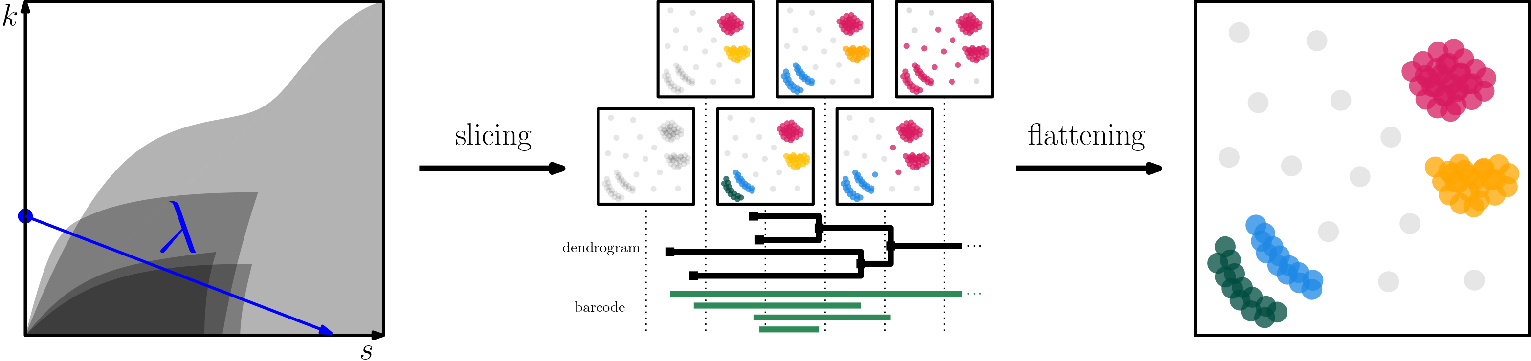
Figure 2: Restricting degree-Rips (Fig. 1) to a line $\lambda$ with negative slope in the degree-Rips parameter space gives a one-parameter hierarchical clustering we call $\lambda$-linkage. The line $\lambda$ lets both of the degree-Rips parameters $s$ and $k$ vary, in contrast to horizontal or vertical lines (see Fig. 1). This allows $\lambda$-linkage to capture multi-scale cluster structure in data, and it leads to better stability properties. The barcode is a visualizable summary of a one-parameter hierarchical clustering. The persistence-based flattening algorithm extracts a single clustering of the underlying data, guided by the barcode.

The Gromov–Hausdorff–Prokhorov stability of degree-Rips is in contrast to the robust single-linkage algorithm and the plug-in algorithm from above, which are discontinuous with respect to the Gromov–Hausdorff–Prokhorov distance, as we show in Section 3.3. In TDA, a standard method for extracting information from a two-parameter persistence module is to take one-parameter slices (see Related Work, below, for references). However, one usually takes slices by lines through the parameter space that do not fix either of the parameters. Slices in which both parameters vary have two key advantages. First, they are multi-scale: they capture information across a range of values of both parameters. Second, these slices have better stability properties, since interleavings between multiparameter persistence modules restrict to interleavings between these slices.

The situation is completely analogous in the setting of hierarchical clustering. So, rather than use robust single-linkage or the plug-in algorithm for density-based clustering (which correspond to using horizontal or vertical slices of degree-Rips), we propose using slices of degree-Rips in which both parameters vary. In more detail, given a line $\lambda$ in the plane with negative slope, restricting $\mathrm{DR}(M)$ to $\lambda$ gives a one-parameter hierarchical clustering, which we call $\lambda$-linkage, denoted $\lambda\textup{-{link}}(M)$ (see Fig. 2). In contrast to robust single-linkage and the plug-in approach, $\lambda$-linkage is multi-scale, and it is stable with respect to the Gromov–Hausdorff–Prokhorov distance: as an immediate corollary of A, we obtain the following stability result.

Result B (Corollary )

Let $\lambda$ be a line in the plane with slope $\sigma<0$. If $M$ and $N$ are finite metric spaces, then

$$d_{\mathrm{CI}}(\lambda\textup{-{link}}(M),\lambda\textup{-{link}}(N))\leq\max(2|\sigma|,1)\cdot d_{\mathrm{GHP}}(M,N)\,.$$

Consistency

Roughly speaking, a “consistency result” for density-based clustering usually says that, given a density function $f$ and an algorithm for computing hierarchical clusterings of finite samples drawn from $f$, the output of the algorithm converges in probability to the density-contour hierarchical clustering $H(f)$, as the sample size goes to infinity. To make this precise, one needs to specify what “converge” means in this context. There is a natural notion of consistency associated to the correspondence-interleaving distance, which we call CI-consistency; the idea is that the output of the algorithm should converge to $H(f)$ in the correspondence-interleaving distance, though in fact we require slightly more than this. CI-consistency is stronger than Hartigan consistency, so proving that an algorithm is CI-consistent implies that it is also Hartigan consistent. While this notion of consistency is novel, we remark that CI-consistency is similar in spirit to the notion of consistency of Eldridge et al. (2015). We prove the following consistency result for $\lambda\textup{-{link}}$. In the statement, the notation $\overline{\lambda}$ indicates that the slice $\lambda\textup{-{link}}$ has been re-parameterized, using an explicit re-parameterization that only depends on $\lambda$; this can be dropped when considering Hartigan consistency, since Hartigan consistency is agnostic to the choice of parameterization.

Result C (Theorem )

The hierarchical clustering algorithm $\overline{\lambda}\textup{-{link}}$ is CI-consistent with respect to any continuous, compactly supported probability density function. In particular, $\lambda\textup{-{link}}$ is Hartigan consistent with respect to any such density function.

Flattening a hierarchical clustering

For many applications, one needs a clustering of the input data, not a hierarchical clustering. We say that a flattening algorithm takes a hierarchical clustering, and returns a single clustering. An example of such a flattening algorithm is the ToMATo clustering algorithm (Chazal et al., 2013), which computes a flattening of the hierarchical clustering induced by a filtered graph. A major advantage of ToMATo is that its output can be understood in terms of the barcode of the input hierarchical clustering. Barcodes are key tools in TDA (Edelsbrunner et al., 2002; Zomorodian and Carlsson, 2005); in this case, the barcode is a visualizable summary of the structure of a one-parameter hierarchical clustering (see Fig. 2). On a technical level however, a disadvantage of ToMATo is that its output depends on a choice of ordering of the vertices in the input graph, and in some use cases there may not be a clear way to make this choice.

We define the persistence-based flattening algorithm (Definition ), an adaptation of the ToMATo algorithm that avoids the dependence on an ordering of the input. And, we prove that it is stable with respect to the correspondence-interleaving distance (Theorem ).

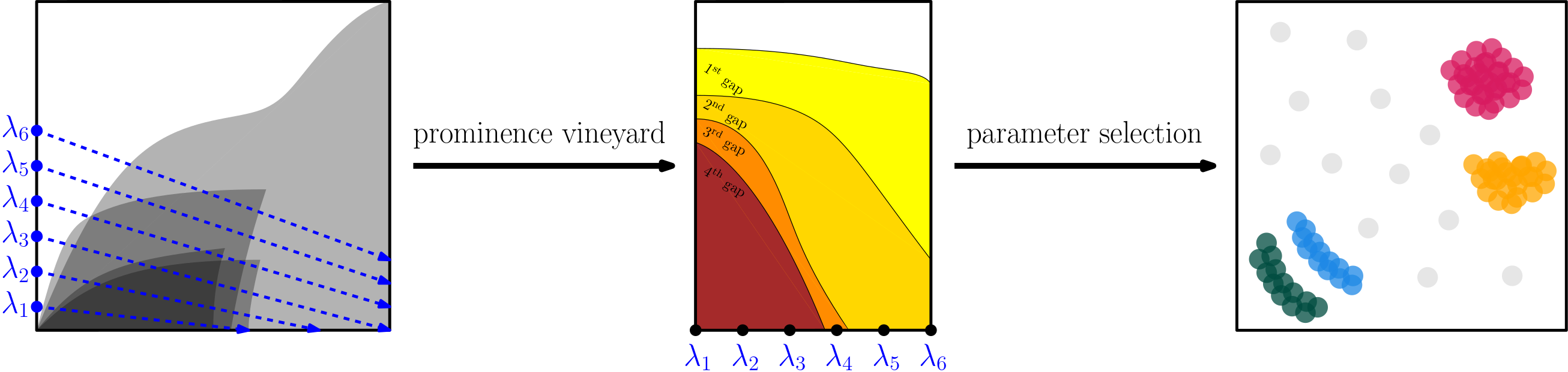
Figure 3: Parameter selection in the Persistable pipeline. The practitioner can choose a slice $\lambda$ using the prominence vineyard. For each $\lambda$ in a chosen family, the prominence vineyard plots the length of each bar in the barcode of $\lambda$-linkage. As $\lambda$ varies continuously, the barcode varies continuously as well. The lengths of the bars trace out continuous curves: the top curve shows the length of the longest bar in the barcode of each slice, the second curve shows the length of the second longest, etc. Choosing a gap in the prominence vineyard leads to a clustering of the data. Larger gaps lead to more stable results.

Persistable

Combining the hierarchical clustering algorithm $\lambda\textup{-{link}}$ and the persistence-based flattening algorithm, we obtain a pipeline for density-based clustering with good stability properties. We call this pipeline Persistable.

Our stability theorems for degree-Rips and the persistence-based flattening algorithm imply theoretical guarantees for the entire pipeline (Corollary  and Corollary ). The stability of degree-Rips also justifies a simple approximation scheme that makes it possible to apply Persistable to large datasets (e.g., the rideshare data in Section 7.2). This approximation scheme is not valid for related methods that are not Gromov–Hausdorff–Prokhorov stable, such as HDBSCAN (Campello et al., 2013) and DBSCAN (Ester et al., 1996).

Persistable includes interactive visualization tools that practitioners can use to choose all parameters in the pipeline. The key task for the practitioner is to choose the slice $\lambda$. Using a vineyard (Cohen-Steiner et al., 2006), one can see how the barcode of $\lambda\textup{-{link}}$ changes with the choice of $\lambda$ (see Fig. 3). Moreover, one can see from the vineyard which choices of $\lambda$ lead to particularly stable clusterings of the input data. We demonstrate Persistable, and this approach to parameter selection, on benchmark datasets, and we show that it provides results that capture meaningful cluster structure. These examples also demonstrate that Persistable can identify multi-scale cluster structure that is challenging for related algorithms, such as HDBSCAN.

HC	Abbreviation for “hierarchical clustering”
Poset of clusterings $\mathsf{C}(X),\preceq$	Definition
The opposite $P^{\mathrm{op}}$ of a poset $P$	Definition
$P$-HC of $X$, $H:P\rightarrow\mathsf{C}(X)$ (with $P$ a poset)	Definition
$n$-parameter HC	Definition
Density-contour HC $H(f)$ of a density $f$	Example
Single-linkage $\mathrm{SL}(M)$ of a metric space $M$	Example
Extension $\bar{H}$ of a HC $H$	Definition
Two HCs are $\vec{\varepsilon}$-interleaved	Definition
The interleaving distance $d_{\mathrm{I}}$	Definition
$\theta_{H}$, ultrametric HC	Definition
Correspondence $R\subseteq X\times Y$, $\pi_{X}:R\rightarrow X$, $\pi_{Y}:R\rightarrow Y$	Definition
Two HCs are $\vec{\varepsilon}$-interleaved w.r.t. $R$	Definition
The correspondence-interleaving distance $d_{\mathrm{CI}}$	Definition
The Hausdorff distance $d_{\mathrm{H}}$	Definition
The Gromov–Hausdorff distance $d_{\mathrm{GH}}$	Definition
metric probability space	Definition
The uniform measure $\mu_{M}$ of $M$	Right below Definition
The uniform filtration $\mathrm{Uni}$	Definition
The degree-Rips HC $\mathrm{DR}$	Definition
A kernel $K$	Definition
The uniform kernel	Example
The local density estimate $\left(\mu_{\mathcal{M}}\ast K_{s}\right)$	Definition
The kernel filtration $\mathcal{M}_{\left[s,k\right]}$ of $\mathcal{M}$	Definition
The kernel linkage $\mathrm{L}^{K}$ or $\mathrm{L}$	Definition
A curve $\gamma$ in a poset, a slice $H^{\gamma}$	Definition
Robust single-linkage $\mathrm{RSL}$	Example
The plug-in algorithm $\mathrm{PI}$	Example
$\lambda$, $\lambda^{x,y}$, $\lambda_{\mathrm{con}}$, $\lambda_{\mathrm{cov}}$, $\lambda\textup{-{link}}$, $\lambda$-linkage	Example
The Prokhorov distance $d_{\mathrm{P}}$	Definition
The Gromov–Hausdorff–Prokhorov distance $d_{\mathrm{GHP}}$	Definition
The Gromov–Hausdorff–Wasserstein distance	Right above Corollary
The closest point correspondence $R_{c}$	Definition
CI-consistency	Definition
The associated cluster tree $\mathcal{F}H$	Example
Hartigan consistency	Definition
$\overline{\lambda}$	Definition
Persistent cluster $\mathbf{C}$, underlying set $U(\mathbf{C})$, $\mathsf{life}$, $\mathsf{birth}$, $\mathsf{length}$	Definition
Poset of persistent clusters $\mathsf{PC}$	Definition
The set of $\mathsf{leaves}$	Definition
Persistence-based pruning $H_{\geq\tau}$	Definition
finite, pointwise finite, essentially finite HC	Definition
The barcode $\mathcal{B}(H)$	Definition
The bottleneck distance $d_{\mathrm{B}}$	Right above Proposition
Prominence diagram	Definition
Prominence diagram $\mathsf{Pr}(H)$ of a HC $H$	Definition  and Definition
Gap $\mathsf{gap}_{n}$, gap size $\mathsf{gapsize}_{n}$	Definition
Gap $\mathsf{gap}_{n}(H)$, gap size $\mathsf{gapsize}_{n}(H)$ of a HC $H$	‣ Section 5.4
Persistence-based flattening $\mathsf{PF}$	Definition
$R_{X}:H(\vec{r})\rightarrow E(\vec{r}+\vec{v}\vec{\varepsilon})$	‣ Section A.5
$B(x,r)$, the open ball of radius $r$ centered at $x$

Definitions and frequently used notation.

Related Work

Distances between (one- and two-parameter) hierarchical clusterings have been studied by Carlsson and Mémoli (2010) and Carlsson and Mémoli (2010). The correspondence-interleaving distance is a generalization of this work; see Section 2.2 for a discussion. The formigram distance, introduced by Kim and Mémoli (2018), can also be seen as a particular instance of the correspondence-interleaving distance. Eldridge et al. (2015) introduce the merge distortion metric for one-parameter hierarchical clusterings, which is closely related to the correspondence-interleaving distance.

Work of Rinaldo et al. (2012) and Chazal et al. (2013) address the stability of consistent hierarchical clustering methods. In their frameworks, stability is guaranteed when their assumptions on the underlying distribution are satisfied. In contrast, our stability results hold without distributional assumptions.

Combining density estimates and graphs that encode distance relations to estimate the density-contour hierarchical clustering has a long history, and several methods based on this idea have been proposed. Along with the work of Cuevas et al. (2000) already mentioned, see, e.g., Biau et al. (2007); Rinaldo and Wasserman (2010); Stuetzle and Nugent (2010); Chazal et al. (2013); Bobrowski et al. (2017).

The consistency of robust single-linkage was first established by Chaudhuri and Dasgupta (2010), and then generalized to density functions supported on manifolds by Balakrishnan et al. (2013). Eldridge et al. (2015) introduced a notion of consistency that is closely related to CI-consistency, and, building on results of Chaudhuri–Dasgupta, they show that robust single-linkage is consistent in this sense.

Multiparameter hierarchical clustering is a topic of increasing interest, as multiparameter hierarchical clusterings have the potential to capture very rich cluster structure in data. See, e.g., Carlsson and Mémoli (2010); Buchin et al. (2015); Kim and Mémoli (2018); Jardine (2019); Bauer et al. (2020); Cai et al. (2020). We expect that the correspondence-interleaving distance will be useful for analyzing the properties of multiparameter hierarchical clustering methods in settings beyond this paper.

As mentioned earlier, our approach to taking slices of the degree-Rips hierarchical clustering is motivated by the standard practice in TDA of studying multiparameter persistence modules via one-parameter slices. See, for example, Cerri et al. (2009); Cagliari et al. (2010); Lesnick and Wright (2015); Landi (2018); Corbet et al. (2019); Vipond (2020); Carrière and Blumberg (2020).

Our notion of rank invariant of a hierarchical clustering is a direct adaptation of the rank invariant of a multiparameter persistence module of Zomorodian and Carlsson (2005). For zero-dimensional homology, which is the relevant context for clustering, the rank invariant was introduced in the earlier work of d’Amico et al. (2003) under the name of size function. The multiparameter version of size functions is due to Biasotti et al. (2008).

When the input data is a finite subset of Euclidean space, and $\gamma$ is a line with constant $s$-component, the algorithm $\gamma\textup{-{link}}$ recovers the connected components of the weighted Čech filtration introduced by Anai et al. (2019), when their parameter $p$ is set to $\infty$. In particular, their stability result applies to this instance of $\gamma\textup{-{link}}$.

As we have already mentioned, the persistence-based flattening we introduce is a modification of the ToMATo clustering algorithm (Chazal et al., 2013). The persistence-based flattening is defined using a pruning procedure we call the persistence-based pruning, which resembles the pruning of Kim et al. (2016).

Blumberg and Lesnick (2022) prove a stability result for the simplicial degree-Rips bifiltration, which we discuss in Remark . Jardine (2020) has also proved results about the stability of degree-Rips, using a hypothesis involving configuration spaces, rather than a distance on metric probability spaces. Scoccola (2020, Section 6.5) shows that results in this paper can be lifted to the stability of the kernel filtration (Definition ), which in particular implies that other topological invariants of this multi-filtration are Gromov–Hausdorff–Prokhorov stable.

2 Hierarchical clustering

The notion of a hierarchical clustering (HC) has been formalized in a variety of ways in the clustering literature. In this section we introduce a new formalization of this notion, which, in particular, allows for HCs with multiple parameters. We introduce the correspondence-interleaving distance between HCs, which generalizes the distance on dendrograms introduced by Carlsson and Mémoli (2010), and we develop its basic properties. In later sections of the paper, we will use the correspondence-interleaving distance to formulate stability and consistency results for hierarchical clustering algorithms.

We also define the degree-Rips and kernel linkage hierarchical clusterings, as well as one-parameter slices of these constructions. These are the basis for all the clustering methods we consider in the rest of the paper.

2.1 The definition of a hierarchical clustering

In order to define the notion of hierarchical clustering, we first define the notion of clustering. See Fig. 8 for an example.

Definition 0

Let $X$ be a set. A clustering of $X$ is a set of non-empty, disjoint subsets of $X$. The elements of a clustering are called clusters.

We will formalize hierarchical clusterings using the notion of a partially ordered set. There are many good references for this notion, for example (Chiossi, 2021, Ch. 2.2.2).

Definition 0

A partially ordered set (poset) is a set $P$ together with a binary relation $\preceq$ such that $(1)$ for all $p\in P$, $p\preceq p$; $(2)$ for all $p,q\in P$, if $p\preceq q$ and $q\preceq p$ then $p=q$; $(3)$ for all $p,q,r\in P$, if $p\preceq q$ and $q\preceq r$ then $p\preceq r$. If $P,Q$ are posets, and $f:P\rightarrow Q$ is a function, then $f$ is order-preserving if for all $p,p^{\prime}\in P$ with $p\preceq p^{\prime}$, $f(p)\preceq f(p^{\prime})$ in $Q$. If $P$ is a poset, the opposite poset $P^{\mathrm{op}}$ is the poset with the same underlying set, and with $p\preceq p^{\prime}$ in $P^{\mathrm{op}}$ if and only if $p\succeq p^{\prime}$ in $P$.

Definition 0

Let $X$ be a set. The poset of clusterings of $X$, denoted $\mathsf{C}(X)$, is the poset whose elements are the clusterings of $X$, and where $S\preceq T\in\mathsf{C}(X)$ if, for each cluster $A\in S$, there is a (necessarily unique) cluster $B\in T$ such that $A\subseteq B$.

Definition 0

Let $P$ be a poset, and let $X$ be a set. A $P$-hierarchical clustering of $X$ is an order-preserving function $H:P\rightarrow\mathsf{C}(X)$.

Definition 0

Let $X$ be a set, and let $n\geq 1$. An $n$-parameter hierarchical clustering of $X$ is a $P$-hierarchical clustering $H:P\rightarrow C(X)$, where $P=I_{1}\times\dots\times I_{n}$ with $I_{j}$ an interval of $\mathbb{R}$ or $\mathbb{R}^{\mathrm{op}}$ for all $1\leq j\leq n$.

Note that one-parameter HCs come in two flavors, depending on whether clusters merge as the real parameter increases or decreases; borrowing terminology from category theory, if $I\subseteq\mathbb{R}$ is an interval, we call an $I$-hierarchical clustering covariant, and if $I\subseteq\mathbb{R}^{\mathrm{op}}$, we call an $I$-hierarchical clustering contravariant. One-parameter HCs can be visualized by dendrograms: see Fig. 4. We now give two key examples of one-parameter HCs.

Example 0

Let $f:\mathbb{R}^{d}\rightarrow\mathbb{R}$ be a probability density function, and let $\mathcal{S}(f)$ be its support. Following Hartigan (1975), the density-contour hierarchical clustering $H(f)$ is the contravariant, $(0,\infty)^{\mathrm{op}}$-hierarchical clustering of $\mathcal{S}(f)$, where, for $r>0$, $H(f)(r)$ is the set of connected components of $\{x\in\mathcal{S}(f)\,:\,f(x)\geq r\}$.

Example 0

Let $M$ be a metric space. The single-linkage hierarchical clustering $\mathrm{SL}(M)$ (Sibson, 1973) is the covariant, $(0,\infty)$-hierarchical clustering of $M$, where, for $r>0$, $\mathrm{SL}(M)(r)$ is the partition of $M$ defined by the smallest equivalence relation $\sim_{r}$ on $M$ with $x\sim_{r}y$ if $d_{M}(x,y)\leq r$. Single-linkage can also be defined in terms of the Rips graph $\mathrm{R}(M)$. For $r>0$, let $\mathrm{R}(M)_{r}$ be the graph with vertex set $M$ and with an edge between $x$ and $y$ if $d_{M}(x,y)\leq r$. Then $\mathrm{SL}(M)(r)$ is the partition of $M$ by the vertex sets of the connected components of $\mathrm{R}(M)_{r}$.

We now describe a way to extend any $n$-parameter hierarchical clustering $H:P\rightarrow\mathsf{C}(X)$ to an $\mathbb{R}^{n}$-hierarchical clustering $\bar{H}:\mathbb{R}^{n}\rightarrow\mathsf{C}(X)$. This will be useful when we consider distances between HCs, since we can compare any two $n$-parameter HCs, with possibly different indexing posets, by first extending them to $\mathbb{R}^{n}$-HCs, and then comparing the extensions. The idea is to first make $H$ covariant in each parameter, by replacing any interval of $\mathbb{R}^{\mathrm{op}}$ in $P$ with its negative, and then to extend $H$ to all of $\mathbb{R}^{n}$ using the empty clustering $\emptyset$ (the minimum in $\mathsf{C}(X)$) and the clustering $\{X\}$ (the maximum in $\mathsf{C}(X)$).

Say $(I,\preceq)\subseteq\mathbb{R}^{\mathrm{op}}$ is an interval: as a set $I$ is a real interval, and $a\preceq b$ in $I$ if and only if $a\geq b$ as real numbers. Let $-I=\{-a:a\in I\}$. There is an isomorphism of posets $\rho_{I}:(-I,\preceq)^{\mathrm{op}}\rightarrow(I,\preceq)$ with $\rho_{I}(a)=-a$, and $(-I,\preceq)^{\mathrm{op}}=(-I,\leq)$ is an interval of $\mathbb{R}$.

Definition 0

Say $P=I_{1}\times\dots\times I_{n}$ with each $I_{j}$ an interval of $\mathbb{R}$ or $\mathbb{R}^{\mathrm{op}}$. Let $P^{\prime}$ be the poset obtained from $P$ by replacing each interval $I_{j}\subseteq\mathbb{R}^{\mathrm{op}}$ with the interval $-I_{j}\subseteq\mathbb{R}$. Then we have an isomorphism of posets $\rho_{P}:P^{\prime}\rightarrow P$. If $X$ is a set, and $H:P\rightarrow\mathsf{C}(X)$ is an $n$-parameter hierarchical clustering of $X$, let $H^{\prime}:P^{\prime}\rightarrow\mathsf{C}(X)$ be $H\circ\rho_{P}$. The extension of $H$ is the $\mathbb{R}^{n}$-hierarchical clustering $\bar{H}:\mathbb{R}^{n}\rightarrow\mathsf{C}(X)$ with

$$\bar{H}(r)=\begin{cases}H^{\prime}(r)&\text{ if $r\in P^{\prime}$}\\ \{X\}&\text{ if $r\in\mathbb{R}^{n}\setminus P^{\prime}$ and there is $p\in P^{\prime}$ with $p<r$}\\ \emptyset&\text{ else}.\end{cases}$$

2.2 The correspondence-interleaving distance

The distances for hierarchical clusterings we consider are based on the notion of interleaving, which we have adapted from persistent homology (Chazal et al., 2009). In the HC setting, interleavings have a simple definition, which we now give.

Notation 0

We write $\vec{\varepsilon}=(\varepsilon_{1},\dots,\varepsilon_{n})\geq\vec{0}$ if $\varepsilon_{i}\geq 0$ for $1\leq i\leq n$.

Definition 0

Let $H$ and $E$ be $n$-parameter hierarchical clusterings of a set $X$, and let $\vec{\varepsilon}\geq\vec{0}$. We say that $H$ and $E$ are $\vec{\varepsilon}$-interleaved if, for all $\vec{r}\in\mathbb{R}^{n}$, we have $\bar{H}(\vec{r})\preceq\bar{E}(\vec{r}+\vec{\varepsilon})$ and $\bar{E}(\vec{r})\preceq\bar{H}(\vec{r}+\vec{\varepsilon})$ in $\mathsf{C}(X)$.

Definition 0

Let $H$ and $E$ be $n$-parameter hierarchical clusterings of a set $X$. Define the interleaving distance

$$d_{\mathrm{I}}(H,E)=\inf\{\varepsilon\geq 0:H,E\text{ are }(\varepsilon,\dots,\varepsilon)\text{-interleaved}\}.$$

In the special case of one-parameter HCs, the interleaving distance has a very concrete, alternative formulation. We give this now, in order to provide intuition for interleavings.

Definition 0

Let $H:I\rightarrow\mathsf{C}(X)$ be a one-parameter hierarchical clustering of a set $X$. Define $\theta_{H}\colon X\times X\rightarrow[-\infty,\infty]$ by $\theta_{H}(x,y)=\inf\{r\in\mathbb{R}:\exists C\in\bar{H}(r),\;x,y\in C\}$. We say $H$ is an ultrametric hierarchical clustering if $I=[0,\infty)$; for all $x\in X$, there is $r_{x}>0$ such that for any $r$ in the interval $[0,r_{x})$, the clustering $H(r)$ contains the singleton cluster $\{x\}$; and there is $r\in[0,\infty)$ such that $H(r)=\{X\}$.

For example, the single-linkage of a finite metric space is an ultrametric hierarchical clustering. If $H$ is an ultrametric hierarchical clustering of $X$, then the function $\theta_{H}$ defines an ultrametric on $X$. See Carlsson and Mémoli (2010) for a detailed discussion of this perspective. For $H,E$ one-parameter HCs of $X$, we write $d_{\infty}(\theta_{H},\theta_{E})=\sup\{|\theta_{H}(x,y)-\theta_{E}(x,y)|:x,y\in X\}$.

Proposition 0

If $H$ and $E$ are one-parameter hierarchical clusterings of a set $X$, then $d_{\mathrm{I}}(H,E)=d_{\infty}(\theta_{H},\theta_{E})$.

The proof is elementary; see Section A.1. This formulation of the interleaving distance shows that, if $H$ and $E$ are $\varepsilon$-interleaved, then the parameter values where clusters are born and merge are perturbed by at most $\varepsilon$. See Fig. 4 for an example. We now give a simple example of a stability result that can be formulated using interleavings.

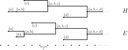
Figure 4: Two dendrograms representing one-parameter, covariant HCs $H$ and $E$ of the set $\{a,b,c,d\}$. The parameter values where points enter the HC, and where clusters merge, are perturbed by at most $\varepsilon$, so the HCs are $\varepsilon$-interleaved.

Proposition 0

Let $f,g:\mathbb{R}^{d}\rightarrow\mathbb{R}_{\geq 0}$ be probability density functions with the same support. Then $d_{\mathrm{I}}(H(f),H(g))=||f-g||_{\infty}$.

We give an elementary proof in Section A.1. This kind of stability result for real-valued functions is standard in topological data analysis. See, for example, Chazal et al. (2016, Example 4.3). We now extend the interleaving distance to HCs of different sets, using correspondences.

Definition 0

A correspondence $R$ between sets $X$ and $Y$ is given by a set $R\subseteq X\times Y$ such that the projections $\pi_{X}:R\rightarrow X$ and $\pi_{Y}:R\rightarrow Y$ are surjective.

If $\psi:Y\rightarrow X$ is a function between sets, and $S=\{C_{i}\}$ is a clustering of $X$, then $\psi^{*}(S)=\{\psi^{-1}(C_{i})\}$ is a clustering of $Y$. This defines an order-preserving map $\psi^{*}:\mathsf{C}(X)\rightarrow\mathsf{C}(Y)$. If $P$ is a poset and $H$ is a $P$-hierarchical clustering of $X$, then $\psi^{*}(H)=\psi^{*}\circ H$ is a $P$-hierarchical clustering of $Y$.

Definition 0

Let $H$ and $E$ be $n$-parameter hierarchical clusterings of sets $X$ and $Y$ respectively, let $R\subseteq X\times Y$ be a correspondence, and let $\vec{\varepsilon}\geq 0$. We say that $H$ and $E$ are $\vec{\varepsilon}$-interleaved with respect to $R$ if $\pi_{X}^{*}(H)$ and $\pi_{Y}^{*}(E)$ are $\vec{\varepsilon}$-interleaved as $n$-parameter hierarchical clusterings of $R$.

Definition 0

Let $H$ and $E$ be $n$-parameter hierarchical clusterings of sets $X$ and $Y$ respectively. Define the correspondence-interleaving distance

$$d_{\mathrm{CI}}(H,E)=\inf_{R}\inf\{\varepsilon\geq 0:H,E\text{ are }(\varepsilon,\dots,\varepsilon)\text{-interleaved w.r.t. }R\}.$$

where the infimum is over all correspondences $R$ between $X$ and $Y$.

Aside from set-theoretic concerns, $d_{\mathrm{CI}}$ defines an extended-pseudo-metric on $n$-parameter hierarchical clusterings (see Section A.1 for the elementary proof):

Proposition 0

The distance $d_{\mathrm{CI}}$ satisfies the following properties, for all $n$-parameter hierarchical clusterings: $(1)$ for any $H$, $d_{\mathrm{CI}}(H,H)=0$; $(2)$ for any $H,E$, $d_{\mathrm{CI}}(H,E)=d_{\mathrm{CI}}(E,H)$; $(3)$ for any $H,E,F$, $d_{\mathrm{CI}}(H,F)\leq d_{\mathrm{CI}}(H,E)+d_{\mathrm{CI}}(E,F)$.

Using correspondences to extend the interleaving distance to HCs of different sets is inspired by the Gromov–Hausdorff distance from metric geometry (Burago et al., 2001, Chapter 7.3). In fact, there is a close connection between the correspondence-interleaving distance and the Gromov–Hausdorff distance. In their work on hierarchical clustering, Carlsson and Mémoli (2010) use the Gromov–Hausdorff distance between the ultrametrics induced by HCs such as the single-linkage HC of a finite metric space. We now recall the definition of the Gromov–Hausdorff distance, and show that the correspondence-interleaving distance recovers this distance, in the special case of ultrametric hierarchical clusterings.

Definition 0

Let $A,B$ be compact subsets of a metric space $M$. The Hausdorff distance between $A$ and $B$ is $d_{\mathrm{H}}^{M}(A,B)=\inf\{\varepsilon>0:A\subseteq B^{\varepsilon}\text{ and }B\subseteq A^{\varepsilon}\}$, where, for any $W\subseteq M$, $W^{\varepsilon}=\{x\in M:\exists w\in W,d_{M}(x,w)<\varepsilon\}$.

Definition 0

Let $M,N$ be compact metric spaces. The Gromov–Hausdorff distance is

$$d_{\mathrm{GH}}(M,N)=\inf_{i,j}\;d_{\mathrm{H}}^{Z}(i(M),j(N))\;,$$

where the infimum is taken over all isometric embeddings $i:M\rightarrow Z$ and $j:N\rightarrow Z$ into a common metric space $Z$.

Proposition 0

Let $H$ and $E$ be ultrametric hierarchical clusterings of sets $X$ and $Y$ respectively. Then $d_{\mathrm{CI}}(H,E)=2\cdot d_{\mathrm{GH}}\left((X,\theta_{H}),(Y,\theta_{E})\right)$.

Proof  Let $R$ be a correspondence between $X$ and $Y$. One says that the distortion of $R$ is $\mathrm{dis}(R)=\sup\{|\theta_{H}(x,x^{\prime})-\theta_{E}(y,y^{\prime})|:(x,y),(x^{\prime},y^{\prime})\in R\}$ (Burago et al., 2001, Definition 7.3.21). Then, one has $d_{\mathrm{GH}}\left((X,\theta_{H}),(Y,\theta_{E})\right)=\frac{1}{2}\inf_{R}\mathrm{dis}(R)$, where the infimum is taken over all correspondences between $X$ and $Y$ (Burago et al., 2001, Theorem 7.3.25). Now, the proposition follows from the fact that, for any correspondence $R$, $\mathrm{dis}(R)=\inf\{\varepsilon\geq 0:H,E\text{ are }\varepsilon\text{-interleaved w.r.t. }R\}$, which is Lemma .  

2.3 Degree-Rips and kernel linkage

We now introduce degree-Rips and kernel linkage, the multiparameter hierarchical clustering methods that are the basis for all the clustering algorithms we consider in this paper. In the introduction, we described degree-Rips in the case that the input is a finite metric space. However, it is very convenient to consider the natural generalization of this construction to metric spaces equipped with a probability measure.

Definition 0

A metric probability space consists of a metric space $\mathcal{M}$ together with a Borel probability measure $\mu_{\mathcal{M}}$ on $\mathcal{M}$.

The degree-Rips hierarchical clustering we define in this section takes a metric probability space as input. If $M$ is a finite metric space, and one equips $M$ with the uniform measure $\mu_{M}$, such that $\mu_{M}(A)=|A|\,/\,|M|$ for any $A\subseteq M$, then the degree-Rips hierarchical clustering of $(M,\mu_{M})$ recovers the version of degree-Rips we described in the introduction. Unless otherwise stated, we equip finite metric spaces with the uniform measure.

Working in the generality of metric probability spaces has two main advantages. First, if $f$ is a density function on Euclidean space, we can consider the degree-Rips hierarchical clustering of the metric probability space $(\mathcal{S}(f),\mu_{f})$, where $\mathcal{S}(f)$ is the support of $f$, and $\mu_{f}$ is the probability measure defined by $f$. This construction plays a key role in the proof of our consistency theorem. Second, finite metric spaces with non-uniform measures are useful for computational purposes. In Section 3.4, we describe an approximation scheme for degree-Rips, in which a large input $M$ (a finite metric space) is approximated by a small subset $N\subset M$, where $N$ has a non-uniform measure that approximates the uniform measure of $M$.

Definition 0

Let $\mathcal{M}$ be a metric probability space, and let $s,k>0$. Let $\mathrm{Uni}(\mathcal{M})_{\left[s,k\right]}=\left\{x\in\mathcal{M}\;:\;\mu_{\mathcal{M}}(B(x,s))\geq k\right\}$. Here and throughout the paper, $B(x,s)$ is the open ball in $\mathcal{M}$ of radius $s$ centered at $x$. We have $\mathrm{Uni}(\mathcal{M})_{\left[s,k\right]}\subseteq\mathrm{Uni}(\mathcal{M})_{\left[s^{\prime},k^{\prime}\right]}$ whenever $s^{\prime}\geq s$ and $k^{\prime}\leq k$. This forms a $2$-parameter filtration of $\mathcal{M}$, which we call the uniform filtration of $\mathcal{M}$.

Blumberg and Lesnick (2022) call this the “measure bifiltration”. We combine the uniform filtration with single-linkage (Example ) to define degree-Rips.

Definition 0

Let $\mathcal{M}$ be a metric probability space. Define the degree-Rips hierarchical clustering of $\mathcal{M}$ as the $2$-parameter hierarchical clustering:

$$\mathrm{DR}(\mathcal{M}):\mathbb{R}_{>0}\times\mathbb{R}_{>0}^{\mathrm{op}} \rightarrow\mathsf{C}(\mathcal{M})$$

$$(s,k) \mapsto\mathrm{SL}\left(\mathrm{Uni}(\mathcal{M})_{\left[s,k\right]}\right)(s)\;.$$

See Fig. 1 for an illustration of degree-Rips. As described in the introduction, we are motivated to consider the degree-Rips hierarchical clustering because of its close connection to well-established methods for data analysis, such as the DBSCAN clustering algorithm and the degree-Rips bifiltration. However, there are some choices baked in to the definition that may not be optimal for some applications. So, we will define a generalization of degree-Rips, which we call kernel linkage.

As motivation, notice that degree-Rips estimates the density near a point $x$ by taking the measure of the ball $B(x,s)$. Equivalently, with respect to the measure $\mu_{\mathcal{M}}$, one integrates the uniform kernel, which is equal to one on this ball and vanishes elsewhere. One could just as well use another kernel when estimating density. Second, notice that the definition of degree-Rips uses the $s$ parameter twice: as the radius of the ball $B(x,s)$, and as the spatial parameter for single-linkage. It is not necessary for these two values to be equal, and in fact, the robust single-linkage algorithm (Example ) allows these two values to differ by a constant factor. These two observations motivate the definition of kernel linkage.

Definition 0

A kernel is a non-increasing function $K:\mathbb{R}_{\geq 0}\rightarrow\mathbb{R}_{\geq 0}$ that is continuous from the right and such that $0<\int_{0}^{\infty}K(r)\,\mathsf{d}r<\infty$.

Note that, in particular, $K(0)>0$ and $\lim_{r\rightarrow\infty}K(r)=0$.

Example 0

Many kernels used for density estimation are kernels in the above sense (see Remark ). We will be particularly interested in $K=\mathbf{1}_{\{r<1\}}:\mathbb{R}_{\geq 0}\rightarrow\mathbb{R}_{\geq 0}$, with $K(x)=1$ if $x<1$ and $K(x)=0$ otherwise. We refer to this as the uniform kernel.

Definition 0

Let $K$ be a kernel, and let $\mathcal{M}$ be a metric probability space. Define the local density estimate of a point $x\in\mathcal{M}$ at scale $s>0$ as

$$\left(\mu_{\mathcal{M}}\ast K_{s}\right)(x):=\int_{x^{\prime}\in\mathcal{M}}K\left(\frac{d_{\mathcal{M}}(x,x^{\prime})}{s}\right)\,\mathsf{d}\mu_{\mathcal{M}}.$$

Remark 0

Let $\mathcal{M}$ be the metric probability space given by Euclidean space $\mathbb{R}^{d}$ equipped with the empirical measure defined by a finite set of points $Z\subset\mathbb{R}^{d}$. The formula for the local density estimate is

$$\left(\mu_{\mathcal{M}}\ast K_{s}\right)(x)=\frac{1}{|Z|}\,\sum_{z\in Z}K\left(\frac{||x-z||}{s}\right)\,.$$

Based on the usual formula for kernel density estimates (Silverman, 1986, Section 4.2.1), one might expect a factor of $1/s^{d}$ here. However, we need our local density estimate to be monotonic in $s$, in order to define the kernel filtration, below. In effect, one can re-introduce the factor $1/s^{d}$ after taking one-parameter slices, and this is what we do to prove our consistency result (see Definition ).

Definition 0

Let $K$ be a kernel, let $\mathcal{M}$ be a metric probability space, and let $s,k>0$. Let $\mathcal{M}_{\left[s,k\right]}=\left\{x\in\mathcal{M}\;:\;\left(\mu_{\mathcal{M}}\ast K_{s}\right)(x)\geq k\right\}$. Note that, since $K$ is non-increasing, we have $\mathcal{M}_{\left[s,k\right]}\subseteq\mathcal{M}_{\left[s^{\prime},k^{\prime}\right]}$ whenever $s^{\prime}\geq s$ and $k^{\prime}\leq k$. This forms a $2$-parameter filtration of $\mathcal{M}$, which we call the kernel filtration of $\mathcal{M}$.

In analogy to the definition of degree-Rips, we combine the kernel filtration with single-linkage to define kernel linkage:

Definition 0

Let $K$ be a kernel, and let $\mathcal{M}$ be a metric probability space. Define the kernel linkage of $\mathcal{M}$ as the $3$-parameter hierarchical clustering of $\mathcal{M}$:

$$\mathrm{L}^{K}(\mathcal{M}):\mathbb{R}_{>0}\times\mathbb{R}_{>0}\times\mathbb{R}_{>0}^{\mathrm{op}} \rightarrow\mathsf{C}(\mathcal{M})$$

$$(s,t,k) \mapsto\mathrm{SL}\left(\mathcal{M}_{\left[s,k\right]}\right)(t)\;.$$

If there is no risk of confusion, we suppress $K$ from the notation, and write $\mathrm{L}(\mathcal{M})$.

To build intuition about kernel linkage, it is helpful to first think about degree-Rips, which is easier to visualize. We provide examples and visualizations in Section 7, where we describe Persistable. The interested reader may wish to look at these visualizations before reading the theoretical material in Section 3.

2.4 Slices of kernel linkage and $\lambda$-linkage

We now formally define the notion of a one-parameter slice of a hierarchical clustering. This is analogous to taking a one-parameter slice of a multiparameter persistence module; see the Related Work section of the introduction for references. Taking one-parameter slices of kernel linkage, one recovers well-known methods for density-based clustering.

Definition 0

Let $P$ be a poset. A curve in $P$ is given by an interval $I_{\gamma}$ of $\mathbb{R}$ or $\mathbb{R}^{\mathrm{op}}$, and an order-preserving function $\gamma:I_{\gamma}\rightarrow P$. If $H:P\rightarrow\mathsf{C}(X)$ is a $P$-hierarchical clustering of a set $X$, and $\gamma:I_{\gamma}\rightarrow P$ is a curve in $P$, then the slice of $H$ by $\gamma$ is the one-parameter hierarchical clustering $H^{\gamma}:I_{\gamma}\rightarrow\mathsf{C}(X)$ given by $H\circ\gamma$.

As discussed in the introduction, some well-known methods for density-based clustering can be recovered by taking slices of kernel linkage.

Example 0

The robust single-linkage algorithm of Chaudhuri and Dasgupta (2010) can be recovered by taking slices of kernel linkage. Let $M$ be a finite metric space with $n=|M|$. Let $\kappa\in\mathbb{N}$ be the density threshold parameter of robust single-linkage, and let $\alpha>0$ be its scale parameter. The robust single-linkage of $M$ is $\mathrm{RSL}_{\kappa,\alpha}(M)=\mathrm{L}^{K}(M)^{\gamma}$, where we take $K$ to be the uniform kernel, and $\gamma$ is the covariant curve $\gamma\colon(0,\infty)\rightarrow\mathbb{R}_{>0}^{\times 3}$ with $\gamma(r)=(r,\alpha r,\kappa/n)$. This is a line through the kernel linkage parameter space, which fixes the density threshold parameter k, and allows the spatial parameters s and t to vary.

Example 0

If we fix the spatial parameters s and t, and allow the density threshold parameter k to vary, we recover the plug-in algorithm for density-based clustering, described in the introduction. See, for example, Cuevas et al. (2000); Chazal et al. (2013). In detail, let $M$ be a finite metric space. For any $s,t>0$, and for any kernel $K$, the plug-in hierarchical clustering of $M$ is $\mathrm{PI}_{s,t}^{K}(M)=\mathrm{L}^{K}(M)^{\gamma}$ for the contravariant curve $\gamma\colon(0,\infty)\rightarrow\mathbb{R}_{>0}^{\times 3}$ with $\gamma(r)=(s,t,r)$.

Slices in which one parameter is fixed, like in the previous two examples, lead to stability problems, as we show in Section 3.3. Moreover, such slices can struggle to capture multi-scale cluster structure in data (see the rideshare data in Section 7.2). So, for Persistable, we use lines in the kernel linkage parameter space in which all parameters vary.

Example 0

For Persistable, we take slices of kernel linkage by a family of curves $\lambda$ that we specify now. See Fig. 2. Each $\lambda$ parameterizes a line in the $(s,k)$-space $\mathbb{R}_{>0}\times\mathbb{R}_{>0}^{\mathrm{op}}$, and we extend this to a curve in the $(s,t,k)$-space $\mathbb{R}_{>0}\times\mathbb{R}_{>0}\times\mathbb{R}_{>0}^{\mathrm{op}}$ by setting $s=t$. We specify a line $\lambda$ by choosing an $s$-intercept $x>0$ and a $k$-intercept $y>0$. We write $\lambda^{x,y}$ if we need to specify the intercepts. Let $\sigma=-y/x$ be the slope of $\lambda$. If we parameterize $\lambda$ with the $k$ coordinate, we get the curve $\lambda_{\mathrm{con}}:(0,y)^{\mathrm{op}}\rightarrow\mathbb{R}_{>0}\times\mathbb{R}_{>0}\times\mathbb{R}_{>0}^{\mathrm{op}}$ defined by $\lambda_{\mathrm{con}}(r)=\left((r/\sigma)+x,\;(r/\sigma)+x,\;r\right)$. If we parameterize with the $s$ coordinate, we get the curve $\lambda_{\mathrm{cov}}:(0,x)\rightarrow\mathbb{R}_{>0}\times\mathbb{R}_{>0}\times\mathbb{R}_{>0}^{\mathrm{op}}$ defined by $\lambda_{\mathrm{cov}}(r)=\left(r,\;r,\;\sigma r+y\right)$.

We say that the $\lambda$-linkage of a metric probability space $\mathcal{M}$ is the hierarchical clustering

$$\lambda\textup{-{link}}(\mathcal{M}):=\mathrm{L}^{K}(\mathcal{M})^{\lambda}$$

where $K$ is the uniform kernel. Since we use the uniform kernel, the slices $\lambda\textup{-{link}}$ are slices of the degree-Rips hierarchical clustering.

When the input is a finite metric space, computing $\lambda$-linkage is similar to computing robust single-linkage. So, one can adapt the algorithms of McInnes and Healy (2018) to compute $\lambda$-linkage. This is what we do for our implementation of Persistable (Scoccola and Rolle, 2023).

3 Stability

In the introduction to this paper, we stated A, which says that the degree-Rips hierarchical clustering method is 2-Lipschitz, with respect to the Gromov–Hausdorff–Prokhorov distance on finite metric spaces, and the correspondence-interleaving distance on hierarchical clusterings. In Section 2.3 we defined the degree-Rips hierarchical clustering not just of a finite metric space, but in the generality of metric probability spaces. In this section, we prove that degree-Rips is 2-Lipschitz for compact metric probability spaces (this includes A as a special case). Furthermore, we consider the kernel linkage construction, also defined in Section 2.3, and show that it is uniformly continuous with respect to the Gromov–Hausdorff–Prokhorov and correspondence-interleaving distances.

3.1 Stability of kernel linkage

We begin by recalling the definition of the Gromov–Hausdorff–Prokhorov distance. We discussed the Hausdorff distance in Section 2.2. The second ingredient we need is the Prokhorov distance (Dudley, 2002, Chapter 11.3).

Definition 0

Let $\mu,\nu$ be Borel probability measures on a metric space $M$. The Prokhorov distance between $\mu$ and $\nu$ is

$$d_{\mathrm{P}}(\mu,\nu)=\inf\{\varepsilon>0\,:\,\mu(A)\leq\nu(A^{\varepsilon})+\varepsilon\;\text{and}\;\nu(A)\leq\mu(A^{\varepsilon})+\varepsilon\text{ for all Borel sets}\;A\subseteq M\}\,.$$

Now, the Gromov–Hausdorff–Prokhorov distance is a metric on the set of isometry-equivalence classes of compact metric probability spaces (see, e.g., Miermont, 2009).

Definition 0

Let $(\mathcal{M},\mu_{\mathcal{M}}),(\mathcal{N},\mu_{\mathcal{N}})$ be compact metric probability spaces. The Gromov–Hausdorff–Prokhorov distance between $(\mathcal{M},\mu_{\mathcal{M}})$ and $(\mathcal{N},\mu_{\mathcal{N}})$ is

$$d_{\mathrm{GHP}}(\mathcal{M},\mathcal{N})=\inf_{i,j}\;\left\{\max(d_{\mathrm{H}}^{Z}(i(\mathcal{M}),j(\mathcal{N})),d_{\mathrm{P}}(i_{*}\mu_{\mathcal{M}},j_{*}\mu_{\mathcal{N}}))\right\}\;,$$

where the infimum is taken over all isometric embeddings $i:\mathcal{M}\rightarrow Z$ and $j:\mathcal{N}\rightarrow Z$ into a common metric space $Z$.

Before proving the stability of kernel linkage, we define a canonical correspondence between two compact metric spaces embedded in a common metric space.

Definition 0

Let $M$ and $N$ be compact metric spaces, let $Z$ be any metric space, and let $i:M\rightarrow Z$ and $j:N\rightarrow Z$ be isometric embeddings. Define the closest point correspondence $R_{c}\subseteq M\times N$, where $(x,y)\in R_{c}$ if and only if $d_{Z}(i(x),j(y))=\min_{y^{\prime}\in N}d_{Z}(i(x),j(y^{\prime}))$ or $d_{Z}(i(x),j(y))=\min_{x^{\prime}\in M}d_{Z}(i(x^{\prime}),j(y))$.

Theorem 0

Kernel linkage is uniformly continuous with respect to the Gromov–Hausdorff–Prokhorov distance on compact metric probability spaces, and the correspondence-interleaving distance. If kernel linkage is defined using the uniform kernel, then it is $2$-Lipschitz.

Proof  Let $K$ be a kernel. We prove the following: for every $\varepsilon>0$, there exists $\delta>0$ such that if $\mathcal{M}$ and $\mathcal{N}$ are compact metric probability spaces and $i:\mathcal{M}\rightarrow Z$ and $j:\mathcal{N}\rightarrow Z$ are isometric embeddings into a metric space $Z$ with $d_{\mathrm{H}}(i(\mathcal{M}),j(\mathcal{N})),d_{\mathrm{P}}(i_{*}\mu_{\mathcal{M}},j_{*}\mu_{\mathcal{N}})<\delta$, then $\mathrm{L}^{K}(\mathcal{M})$ and $\mathrm{L}^{K}(\mathcal{N})$ are $(\varepsilon,\varepsilon,\varepsilon)$-interleaved with respect to the closest point correspondence $R_{c}\subseteq\mathcal{M}\times\mathcal{N}$.

Let $r^{\prime}\in(0,K(0))$ and $\delta>0$, and define $\delta_{s}=\frac{2\delta}{K^{-1}(r^{\prime})}$ and $\delta_{k}=K(0)^{2}/r^{\prime}-K(0)+K(0)\delta$. We now prove that if $\mathcal{M}$ and $\mathcal{N}$ are compact metric probability spaces and $i:\mathcal{M}\rightarrow Z$ and $j:\mathcal{N}\rightarrow Z$ are isometric embeddings with $d_{\mathrm{H}}(i(\mathcal{M}),j(\mathcal{N})),d_{\mathrm{P}}(i_{*}\mu_{\mathcal{M}},j_{*}\mu_{\mathcal{N}})<\delta$, then $\mathrm{L}^{K}(\mathcal{M})$ and $\mathrm{L}^{K}(\mathcal{N})$ are $(\delta_{s},2\delta,\delta_{k})$-interleaved with respect to $R_{c}$. This implies the statement of the previous paragraph, by taking $r^{\prime}\in(0,K(0))$ such that $K(0)^{2}/r^{\prime}-K(0)<\varepsilon/2$, and $\delta>0$ such that $2\delta/K^{-1}(r^{\prime})<\varepsilon$, $2\delta<\varepsilon$, and $K(0)\delta<\varepsilon/2$.

It suffices to show that, for any $s,t>0$ and $k>\delta_{k}$, we have relations in $\mathsf{C}(R_{c})$:

$$\pi_{\mathcal{M}}^{*}\left(\mathrm{L}^{K}(\mathcal{M})\right)(s,t,k) \preceq\pi_{\mathcal{N}}^{*}\left(\mathrm{L}^{K}(\mathcal{N})\right)(s+\delta_{s},t+2\delta,k-\delta_{k})$$

$$\pi_{\mathcal{N}}^{*}\left(\mathrm{L}^{K}(\mathcal{N})\right)(s,t,k) \preceq\pi_{\mathcal{M}}^{*}\left(\mathrm{L}^{K}(\mathcal{M})\right)(s+\delta_{s},t+2\delta,k-\delta_{k})\,.$$

We show that the first relation holds, and the second relation follows from a symmetric argument. Let $(x,y)\in R_{c}$. If $(x,y)$ belongs to a cluster of $\pi_{\mathcal{M}}^{*}(\mathrm{L}^{K}(\mathcal{M}))(s,t,k)$, then it belongs to a cluster of $\pi_{\mathcal{N}}^{*}(\mathrm{L}^{K}(\mathcal{N}))(s+\delta_{s},t+2\delta,k-\delta_{k})$, by Lemma . Now, assume that $(x,y)$ and $(x^{\prime},y^{\prime})\in R_{c}$ belong to the same cluster in $\pi_{\mathcal{M}}^{*}(\mathrm{L}^{K}(\mathcal{M}))(s,t,k)$. This means that $x\sim_{t}x^{\prime}$ in $\mathcal{M}_{\left[s,k\right]}$. Since $|d_{\mathcal{M}}(x_{1},x_{2})-d_{\mathcal{N}}(y_{1},y_{2})|<2\delta$ for every $(x_{1},y_{1}),(x_{2},y_{2})\in R_{c}$, we have that $y\sim_{t+2\delta}y^{\prime}$ in $\mathcal{N}_{\left[s+\delta_{s},k-\delta_{k}\right]}$ as required.

It remains to consider the case where $K$ is the uniform kernel. Then $K(0)=1$, and, for every $r^{\prime}\in(0,1)$ we have $K^{-1}(r^{\prime})=1$, since $K^{-1}=K$. Letting $r^{\prime}\rightarrow 1$, the interleaving we constructed above approaches a $(2\delta,2\delta,\delta)$-interleaving, as needed.  

Corollary 0

If $\mathcal{M}$ and $\mathcal{N}$ are compact metric probability spaces, then

$$d_{\mathrm{CI}}(\mathrm{DR}(\mathcal{M}),\mathrm{DR}(\mathcal{N}))\leq 2\cdot d_{\mathrm{GHP}}(\mathcal{M},\mathcal{N})\,.$$

Proof  Since degree-Rips is defined using the uniform kernel, it is $2$-Lipschitz by Theorem .  

Theorem  implies a similar result for the Gromov–Hausdorff–Wasserstein distance, which is defined just as in Definition , except one replaces the Prokhorov distance with the Wasserstein distance (Gibbs and Su, 2002, p. 424).

Corollary 0

Kernel linkage is uniformly continuous with respect to the Gromov–Hausdorff–Wasserstein distance on compact metric probability spaces, and the correspondence-interleaving distance.

Proof  By Gibbs and Su (2002, Theorem 2), if $\mu$ and $\nu$ are probability measures on a compact metric space, then $d_{\mathrm{P}}(\mu,\nu)^{2}\leq d_{\mathrm{W}}(\mu,\nu)$, where $d_{\mathrm{W}}$ denotes the Wasserstein distance. Now the corollary follows immediately from Theorem .  

Remark 0

We now discuss why we use the Gromov–Hausdorff–Prokhorov distance for analyzing the stability of the degree-Rips and kernel linkage hierarchical clusterings. Because these constructions are density-sensitive, they are not continuous with respect to the Gromov–Hausdorff distance, unlike single-linkage (Carlsson and Mémoli, 2010). They are also not continuous with respect to the Gromov–Prokhorov distance. This was observed for the simplicial degree-Rips bifiltration by Blumberg and Lesnick (2022, Remark 3.8), using the homotopy interleaving distance on simplicial bifiltrations. The same example shows that the degree-Rips hierarchical clustering is not continuous with respect to the Gromov–Prokhorov distance on finite metric spaces (equipped with the uniform measure) and the correspondence-interleaving distance. However, as we have shown, if one uses the Gromov–Hausdorff–Prokhorov distance, degree-Rips is continuous, and even Lipschitz.

We note that Blumberg and Lesnick (2022, Theorem 1.7) prove a Gromov–Prokhorov stability result for the simplicial degree-Rips bifiltration using homotopy interleavings. Necessarily, the conclusion is weaker than continuity. This stability result is complementary to our results. By working with the Gromov–Prokhorov distance, they make weaker assumptions on the input, and get correspondingly weaker conclusions.

3.2 Stability of slices of kernel linkage

Interleavings between multiparameter hierarchical clusterings restrict to interleavings between slices, provided the slice does not fix any parameters. This is analogous to the behavior of interleavings and slices of multiparameter persistence modules; see the Related Work section of the Introduction for references.

Because the curves $\lambda$ that we use for Persistable (Example ) allow all parameters of kernel linkage to vary, we get Gromov–Hausdorff–Prokhorov stability for $\lambda\textup{-{link}}$ as an immediate corollary of Theorem .

Corollary 0

Let $\lambda=\lambda^{x,y}$ for $x,y>0$, and let $\sigma$ be the slope of $\lambda$. Then, with respect to the Gromov–Hausdorff–Prokhorov distance on compact metric probability spaces and the correspondence-interleaving distance:

1. $\lambda_{\mathrm{con}}\textup{-{link}}$ is $\max(2|\sigma|,1)$-Lipschitz,

2. $\lambda_{\mathrm{cov}}\textup{-{link}}$ is $\max(|1/\sigma|,2)$-Lipschitz.

Proof  If $\mathcal{M}$ and $\mathcal{N}$ are compact metric probability spaces and $\delta>d_{\mathrm{GHP}}(\mathcal{M},\mathcal{N})$, then the proof of Theorem  shows that $\mathrm{L}(\mathcal{M})$ and $\mathrm{L}(\mathcal{N})$ are $(2\delta,2\delta,\delta)$-interleaved with respect to the closest-point correspondence. Restricting this interleaving to the line $\lambda$, as in e.g. Landi (2018, Lemma 1), we get the required interleavings.  

Based on this result, we say that $\lambda_{\mathrm{con}}\textup{-{link}}$ and $\lambda_{\mathrm{cov}}\textup{-{link}}$ are stable with respect to the Gromov–Hausdorff–Prokhorov distance. The slices $\lambda_{\mathrm{con}}\textup{-{link}}$ and $\lambda_{\mathrm{cov}}\textup{-{link}}$ are also stable in the choice of $\lambda$:

Proposition 0

Let $\mathcal{M}$ be a metric probability space. Let $\lambda=\lambda^{x,y}$ with slope $\sigma=-y/x$ be defined by intercepts $x,y>0$, and let $\lambda^{\prime}=\lambda^{x^{\prime},y^{\prime}}$ with slope $\sigma^{\prime}=-y^{\prime}/x^{\prime}$ be defined by intercepts $x^{\prime},y^{\prime}>0$.

1. $d_{\mathrm{CI}}\left(\lambda_{\mathrm{con}}\textup{-{link}}(\mathcal{M}),\lambda^{\prime}_{\mathrm{con}}\textup{-{link}}(\mathcal{M})\right)\leq\max\left(|y-y^{\prime}|,\;|x-x^{\prime}|\cdot\min(|\sigma|,|\sigma^{\prime}|)\right)$.

2. $d_{\mathrm{CI}}\left(\lambda_{\mathrm{cov}}\textup{-{link}}(\mathcal{M}),\lambda^{\prime}_{\mathrm{cov}}\textup{-{link}}(\mathcal{M})\right)\leq\max\left(|x-x^{\prime}|,\;|y-y^{\prime}|\cdot\min(|1/\sigma|,|1/\sigma^{\prime}|)\right)$.

Proof  One can construct the required interleavings as in e.g. Landi (2018, Lemma 2).  

3.3 Instability of related methods

In the introduction, we discussed two well-known methods for density-based clustering, which can be recovered by taking slices of kernel linkage; these are robust single-linkage (Example ) and the plug-in algorithm (Example ). In contrast to the hierarchical clusterings $\lambda\textup{-{link}}$ we use for Persistable, we now show that these methods are discontinuous with respect to the Gromov–Hausdorff–Prokhorov distance.

We begin with robust single-linkage. If one fixes the robust single-linkage parameters $\kappa\in\mathbb{N}$ and $\alpha>0$, then one can think of robust single-linkage $\mathrm{RSL}_{\kappa,\alpha}$ as a function that takes a finite metric space as input and produces a one-parameter hierarchical clustering as output, and this function is discontinuous:

Proposition 0

Let $\kappa\geq 2$ and $\alpha>0$. With respect to the Gromov–Hausdorff–Prokhorov distance and the correspondence-interleaving distance, $\mathrm{RSL}_{\kappa,\alpha}$ is discontinuous.

We prove this by giving a simple example in Section A.2. One could also formalize robust single-linkage differently, taking the density threshold parameter to be a ratio $k\in(0,1)$, and then letting $\mathrm{RSL}_{k,\alpha}(M)=\mathrm{L}(M)^{\gamma}$ for the covariant curve $\gamma\colon(0,\infty)\rightarrow\mathbb{R}_{>0}^{\times 3}$ with $\gamma(r)=(r,\alpha r,k)$. We show in Section A.2 that this variant is also discontinuous with respect to the Gromov–Hausdorff–Prokhorov distance.

In contrast to the stability of $\lambda\textup{-{link}}$ in $\lambda$ (Proposition ), changing the density threshold parameter $\kappa$ of robust single-linkage can lead to arbitrarily large changes in the output:

Proposition 0

Let $\kappa,\kappa^{\prime}\in\mathbb{N}$ with $\kappa\neq\kappa^{\prime}$, and let $\alpha>0$. For any $D>0$, there is a finite metric space $M$ such that $d_{\mathrm{CI}}(\mathrm{RSL}_{\kappa,\alpha}(M),\mathrm{RSL}_{\kappa^{\prime},\alpha}(M))>D$.

There is an analogous result for the variant of robust single-linkage that takes a density threshold $k\in(0,1)$ instead of $\kappa$. See Section A.2.

We now consider the plug-in algorithm. As before, if one fixes the parameters $s,t>0$, then $\mathrm{PI}_{s,t}$ is a function that takes a finite metric space as input and produces a one-parameter hierarchical clustering as output, and we have the following:

Proposition 0

Let $s,t>0$, and let $\mathrm{PI}$ be defined using any kernel. With respect to the Gromov–Hausdorff–Prokhorov distance and the correspondence-interleaving distance, $\mathrm{PI}_{s,t}$ is discontinuous.

We prove this in Section A.2 by giving a simple example. Finally, we consider the instability of the plug-in algorithm in its parameters. For a fixed metric probability space $\mathcal{M}$, Proposition  implies that (in both the covariant and contravariant versions) $\lambda\textup{-{link}}(\mathcal{M})$ is continuous as a function from its parameter space $\{\lambda^{x,y}\}_{x,y>0}$ to the space of one-parameter hierarchical clusterings endowed with the correspondence-interleaving distance. Similarly, if we fix a finite metric space $M$, then the plug-in algorithm can be seen as a function $\mathrm{PI}_{-,-}(M)$ that takes input $s,t>0$ and produces a one-parameter hierarchical clustering as output. However, this is not continuous (see Section A.2 for the proof):

Proposition 0

Let $\mathrm{PI}$ be defined using any kernel, and let $M$ be any finite metric space with $|M|\geq 2$. Then $\mathrm{PI}_{-,-}(M)$ is discontinuous, with respect to the Euclidean distance on $\mathbb{R}_{>0}^{2}$ and the correspondence-interleaving distance.

3.4 Approximation of $\lambda$-linkage by subsampling

Because degree-Rips and $\lambda$-linkage are Gromov–Hausdorff–Prokhorov stable, they admit a very simple approximation algorithm. For example, say $\lambda=\lambda_{\mathrm{con}}$, and we want to compute $\lambda\textup{-{link}}(M)$, where $M$ is a finite metric space, equipped with the uniform measure. Say $N\subset M$ is a subsample, with $\varepsilon=d_{\mathrm{H}}(M,N)$. Then, by Proposition , one can compute a probability measure on $N$ such that $d_{\mathrm{GHP}}(M,N)\leq\varepsilon$, and therefore, by Corollary , we have $d_{\mathrm{CI}}(\lambda\textup{-{link}}(M),\lambda\textup{-{link}}(N))\leq\max(2|\sigma|,1)\cdot\varepsilon$.

Therefore, if we can find a small subsample of $M$ that is close in the Hausdorff distance, we need only compute $\lambda\textup{-{link}}$ of the subsample in order to approximate $\lambda\textup{-{link}}(M)$. Persistable implements several subsampling methods, which can be used to get fast results on large datasets. We present an example in Section 7.

Proposition 0

Let $(\mathcal{M},\mu_{\mathcal{M}})$ be a finite metric probability space. Let $\mathcal{N}\subseteq\mathcal{M}$ be a subset and let $i:\mathcal{N}\rightarrow\mathcal{M}$ denote the inclusion. Choose any function $f:\mathcal{M}\rightarrow\mathcal{N}$ with the property that, for every $x\in\mathcal{M}$, the point $f(x)\in\mathcal{N}$ is a closest point of $\mathcal{N}$ to $x$. Define a probability measure on $\mathcal{N}$ by $\mu_{\mathcal{N}}=f_{*}(\mu_{\mathcal{M}})$. Then $d_{\mathrm{P}}(\mu_{\mathcal{M}},i_{*}\mu_{\mathcal{N}})\leq d_{\mathrm{H}}(\mathcal{M},\mathcal{N})$ and, in particular, $d_{\mathrm{GHP}}(\mathcal{M},\mathcal{N})\leq d_{\mathrm{H}}(\mathcal{M},\mathcal{N})$.

Proof  Let $\varepsilon>0$ be such that $\mathcal{M}\subseteq\mathcal{N}^{\varepsilon}$; it is enough to show that $d_{\mathrm{P}}(\mu_{\mathcal{M}},i_{*}\mu_{\mathcal{N}})\leq\varepsilon$. We prove that, for every $A\subseteq\mathcal{M}$ we have $\mu_{\mathcal{M}}(A)\leq\mu_{\mathcal{N}}(A^{\varepsilon})$ and $\mu_{\mathcal{N}}(A)\leq\mu_{\mathcal{M}}(A^{\varepsilon})$.

Note that $d_{\mathcal{M}}(x,f(x))\leq\varepsilon$ for all $x\in\mathcal{M}$. It follows that $f^{-1}(A\cap\mathcal{N})\subseteq A^{\varepsilon}$ and $f(A)\subseteq A^{\varepsilon}\cap\mathcal{N}$ for all $A\subseteq\mathcal{M}$. Note also that $i_{*}\mu_{\mathcal{N}}(B)=\mu_{\mathcal{M}}(f^{-1}(B\cap\mathcal{N}))$ for every $B\subseteq\mathcal{M}$, by definition of $i_{*}$ and $f_{*}$. Let $A\subseteq\mathcal{M}$. Using the above, we get on one hand $i_{*}\mu_{\mathcal{N}}(A)=\mu_{\mathcal{M}}(f^{-1}(A\cap\mathcal{N}))\leq\mu_{\mathcal{M}}(A^{\varepsilon})$. On the other hand, $A\subseteq f^{-1}(f(A))\subseteq f^{-1}(A^{\varepsilon}\cap\mathcal{N})$, and thus $\mu_{\mathcal{M}}(A)\leq\mu_{\mathcal{M}}(f^{-1}(A^{\varepsilon}\cap\mathcal{N}))=i_{*}\mu_{\mathcal{N}}(A^{\varepsilon})$.  

4 Consistency

There is a natural notion of consistency for hierarchical clustering algorithms associated to the correspondence-interleaving distance. In this section, we define this, show that it implies Hartigan consistency, and show that $\lambda$-linkage is consistent with respect to the correspondence-interleaving distance.

In this section, unless otherwise stated, a hierarchical clustering will be a one-parameter hierarchical clustering (Definition ).

4.1 Notions of consistency of hierarchical clustering algorithms

Definition 0

A hierarchical clustering algorithm $\mathbb{A}$ with parameter space $\Theta$ is a mapping that assigns to each finite metric space $M$ and each parameter $\theta\in\Theta$ a hierarchical clustering $\mathbb{A}^{\theta}(M)$ of $M$.

We now define the notion of consistency associated to the correspondence-interleaving distance, using the density-contour hierarchical clustering $H(f)$ (Example ) and the closest point correspondence $R_{c}$ (Definition ).

Definition 0

Let $f:\mathbb{R}^{d}\rightarrow\mathbb{R}$ be a probability density function with support $\mathcal{S}(f)$. A hierarchical clustering algorithm $\mathbb{A}$ with parameter space $\Theta$ is CI-consistent with respect to $f$ if for every $n\in\mathbb{N}$ there exists a parameter $\theta_{n}\in\Theta$ such that, for every $\varepsilon>0$ and $X_{n}$ an i.i.d. $n$-sample of $\mathcal{S}(f)$ with distribution $f$, the probability that $\mathbb{A}^{\theta_{n}}(X_{n})$ and $H(f)$ are $\varepsilon$-interleaved with respect to $R_{c}$ goes to $1$ as $n$ goes to $\infty$.

Remark 0

In practice, one may want an explicit rule for choosing the parameters $\theta_{n}$ of Definition  as a function of $n$. Moreover, one may also want rates of convergence for the algorithm. Although we do not specifically address this in this paper, we mention that such results can be extracted from the proof of the consistency result Theorem  together with rates of convergence of samples in the Hausdorff distance (Cuevas and Rodríguez-Casal, 2004) and in the Prokhorov distance (Dudley, 1969).

We now define Hartigan consistency, following Hartigan (1981).

Definition 0

Let $X$ be a set. A cluster tree of $X$ is given by a family $\mathcal{T}$ of subsets of $X$ with the property that whenever $A$ and $B$ are distinct elements of $\mathcal{T}$, then one of the following is true: $A\cap B=\emptyset$, $A\subseteq B$, or $B\subseteq A$. The elements of $\mathcal{T}$ are called clusters.

Example 0

Let $H:I\rightarrow\mathsf{C}(X)$ be a hierarchical clustering of a set $X$. We can define an associated cluster tree $\mathcal{F}H=\{C\in H(r):r\in I\}$.

Definition 0

A cluster tree algorithm $\mathbb{A}$ with parameter space $\Theta$ is a mapping that assigns to each finite metric space $M$ and each parameter $\theta\in\Theta$ a cluster tree $\mathbb{A}^{\theta}(M)$ of $M$.

Definition 0 (cf. Hartigan, 1981)

Let $f:\mathbb{R}^{d}\rightarrow\mathbb{R}$ be a probability density function with support $\mathcal{S}(f)$. A cluster tree algorithm $\mathbb{A}$ with parameter space $\Theta$ is Hartigan consistent with respect to $f$ if for every $n\in\mathbb{N}$ there exists a parameter $\theta_{n}\in\Theta$ such that, given $A$ and $A^{\prime}$ distinct elements of $H(f)(r)$ for some $r>0$, and $X_{n}$ an i.i.d. $n$-sample of $\mathcal{S}(f)$ with distribution $f$ we have

$$P(A_{n}\cap A^{\prime}_{n}=\emptyset)\xrightarrow{n\rightarrow\infty}1,$$

where $A_{n}$ is the smallest cluster in $\mathbb{A}^{\theta_{n}}(X_{n})$ that contains $A\cap X_{n}$, and $A^{\prime}_{n}$ is the smallest cluster in $\mathbb{A}^{\theta_{n}}(X_{n})$ that contains $A^{\prime}\cap X_{n}$.

The proof of the following result is in Section A.3.

Proposition 0

Let $f:\mathbb{R}^{d}\rightarrow\mathbb{R}$ be a continuous and compactly supported probability density function. If a hierarchical clustering algorithm $\mathbb{A}$ is CI-consistent with respect to $f$, then the associated cluster tree algorithm $\mathcal{F}\mathbb{A}$ is Hartigan consistent with respect to $f$.

4.2 Consistency of $\lambda$-linkage

Let $f:\mathbb{R}^{d}\rightarrow\mathbb{R}$ be a continuous and compactly supported probability density function with support $\mathcal{S}(f)$, and let $\mu_{f}$ be the probability measure defined by $f$. We now prove that the hierarchical clustering algorithm $\lambda\textup{-{link}}$ is CI-consistent with respect to $f$. The strategy is to construct an interleaving between $H(f)$ and the $\lambda\textup{-{link}}$ of the metric probability space $(\mathcal{S}(f),\mu_{f})$. Then, the stability of $\lambda\textup{-{link}}$ implies that, for a sufficiently good sample $X_{n}$ of $f$, the $\lambda\textup{-{link}}$ of $X_{n}$ is a good approximation of the $\lambda\textup{-{link}}$ of $(\mathcal{S}(f),\mu_{f})$.

However, in order to interleave $\lambda\textup{-{link}}$ and $H(f)$, we must first reparameterize $\lambda\textup{-{link}}$, as discussed in Remark .

Definition 0

Let $\lambda=\lambda_{\mathrm{con}}^{x,y}$ for $x,y>0$ (see Example ). For $s>0$, we write $v_{s}$ for the volume of a ball in $\mathbb{R}^{d}$ of radius $s$. Define an order-preserving function $\varphi:(0,y)^{\mathrm{op}}\rightarrow\mathbb{R}_{>0}^{\mathrm{op}}$ by $\varphi(r)=\frac{r}{v_{\lambda_{s}(r)}}$. Note that $\varphi$ is a bijection; we write $\overline{\lambda}=\lambda\circ\varphi^{-1}$. For any metric probability space $\mathcal{M}$, we write $\overline{\lambda}\textup{-{link}}(\mathcal{M})=\mathrm{L}^{K}(\mathcal{M})^{\overline{\lambda}}$, with $K$ the uniform kernel.

Theorem 0

The hierarchical clustering algorithm $\overline{\lambda}\textup{-{link}}$ with parameter space $\{\lambda_{\mathrm{con}}^{x,y}\}_{x,y>0}$ is CI-consistent with respect to any continuous, compactly supported probability density function $f:\mathbb{R}^{d}\rightarrow\mathbb{R}$.

This is a special case of Theorem , which is proved in Section A.3.

Remark 0

For any $\lambda\in\{\lambda_{\mathrm{con}}^{x,y}\}_{x,y>0}$, $\lambda\textup{-{link}}$ and $\overline{\lambda}\textup{-{link}}$ produce the same underlying cluster tree. So, it follows from the preceding theorem that the algorithm $\lambda\textup{-{link}}$ with parameter space $\{\lambda_{\mathrm{con}}^{x,y}\}_{x,y>0}$ is Hartigan consistent with respect to any continuous, compactly supported probability density function $f:\mathbb{R}^{d}\rightarrow\mathbb{R}$.

5 Structure of one-parameter hierarchical clusterings

Barcodes are used in topological data analysis to summarize structural information about data (Edelsbrunner et al., 2002; Zomorodian and Carlsson, 2005). Since they were first introduced, a rich theory has been developed for barcodes (see e.g., Chazal et al. 2016). Barcodes can be defined in many different contexts, and are used to summarize various geometric and topological properties of different kinds of data. In particular, one-parameter hierarchical clusterings have barcodes, and these are a key ingredient in the Persistable pipeline. See Fig. 5 for an example of a barcode.

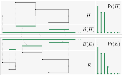
Figure 5: The barcode $\mathcal{B}(H)$ of a hierarchical clustering $H$ is a collection of real intervals, called bars (displayed in green). Informally, the barcode is constructed using the following two rules: (1) If a new cluster enters $H$ at parameter $r$, start a new bar with left endpoint $r$. (2) If two clusters merge at $r$, take the cluster that entered the hierarchy later (i.e., at a larger parameter value), and end its bar at $r$. The second rule is called the Elder rule, since the elder bar survives. In the case of HCs induced by filtered graphs, we give a precise formulation of the Elder rule and prove its correctness (Algorithm 1). A matching is shown between the barcodes of $H$ and $E$. The prominence diagram $\mathsf{Pr}(H)$ is simply the data of the lengths of the bars in $\mathcal{B}(H)$ (Section 5.4).

Barcodes of hierarchical clusterings and related structures are a standard topic in topological data analysis (see e.g. Curry 2018; Cai et al. 2020; Dey and Wang 2022, Section 3.5.3). A key point is that the so-called “Elder rule” can be used to efficiently compute the barcode. However, to the best of our knowledge, there is no source in the literature that proves the correctness of the Elder rule in the generality we require. Because the barcode is a key component of Persistable, and because we believe barcodes are an important tool for anyone working with hierarchical clusterings, in this section we give a detailed treatment of this topic. Along with the barcode, we consider a closely related structure, which we call the poset of persistent clusters. Some readers may wish to skim this section on a first reading of the paper, and refer to it as needed when encountering barcodes.

5.1 The poset of persistent clusters

We now define a fundamental object associated to a hierarchical clustering, which we call the poset of persistent clusters (see Fig. 6 for an illustration). This object, or something equivalent, appears in many places (e.g., Kim et al., 2016, Appendix A; McInnes and Healy, 2018, Section 2.3; Jardine, 2019). We first define the notion of persistent cluster.

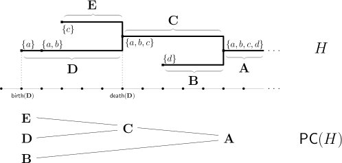
Figure 6: For the hierarchical clustering $H$, the poset of persistent clusters $\mathsf{PC}(H)$ is the poset with elements $\mathbf{A},\mathbf{B},\mathbf{C},\mathbf{D},\mathbf{E}$, where $\mathbf{E},\mathbf{D}<\mathbf{C}$, etc. The leaves of $H$ are $\mathbf{E},\mathbf{D}$, and $\mathbf{B}$. The parameter values $\mathsf{birth}(\mathbf{D})$ and $\mathsf{death}(\mathbf{D})$ are marked; the underlying set of $\mathbf{D}$ is $U(\mathbf{D})=\{a,b\}$.

Definition 0

Let $X$ be a set. A persistent cluster $\mathbf{C}$ of $X$ consists of an interval $\mathsf{life}(\mathbf{C})\subseteq\mathbb{R}$ together with an order-preserving function $\mathbf{C}:\mathsf{life}(\mathbf{C})\rightarrow\mathcal{P}(X)$, where $\mathcal{P}(X)$ is the power set of $X$ ordered by inclusion. The underlying set of the persistent cluster $\mathbf{C}$ is $U(\mathbf{C})=\cup_{r\in\mathsf{life}(\mathbf{C})}\mathbf{C}(r)$, and two persistent clusters are disjoint if their underlying sets are disjoint. Let $\mathsf{birth}(\mathbf{C})=\inf\mathsf{life}(\mathbf{C})$, $\mathsf{death}(\mathbf{C})=\sup\mathsf{life}(\mathbf{C})$, and $\mathsf{length}(\mathbf{C})=\mathsf{death}(\mathbf{C})-\mathsf{birth}(\mathbf{C})$.

We remark that persistent clusters are, in particular, one-parameter hierarchical clusterings, so one can consider interleavings between persistent clusters.

Definition 0

Let $I\subseteq\mathbb{R}$ be an interval and let $H$ be an $I$-hierarchical clustering. The underlying set of the poset of persistent clusters of $H$, denoted $\mathsf{PC}(H)$, is the quotient set $\left(\coprod_{r\in I}H(r)\right)/\sim$ where:

• The set $\coprod_{r\in I}H(r)$ denotes the disjoint union of all clusterings as $r$ varies in $I$.

• The relation $\sim$ is the symmetric closure of the following relation. For $r_{1}\leq r_{2}$, $C_{1}\in H(r_{1})$, and $C_{2}\in H(r_{2})$, we have that $C_{1}$ and $C_{2}$ are related if and only if $C_{1}\subseteq C_{2}$ and, for every $r_{3}\in[r_{1},r_{2}]$, there is exactly one cluster $C_{3}\in H(r_{3})$ such that $C_{3}\subseteq C_{2}$.

Let $\mathbf{C}\in\mathsf{PC}(H)$. The equivalence class $\mathbf{C}$ is naturally a persistent cluster in the sense of Definition , with $\mathsf{life}(\mathbf{C})=\{r\in I:\exists C\in H(r)\;\text{with}\;\mathbf{C}=[C]\}$ and such that, for $r\in\mathsf{life}(\mathbf{C})$, we let $\mathbf{C}(r)=C$, with $C\in H(r)$ the only cluster in $H(r)$ such that $[C]=\mathbf{C}$. With this in mind, we define the partial order on $\mathsf{PC}(H)$ by letting $\mathbf{C}\leq\mathbf{D}$ if $U(\mathbf{C})\subseteq U(\mathbf{D})$.

The second poset axiom (Definition ) for $\mathsf{PC}(H)$ is established in Lemma . The other poset axioms follow immediately from the definition. See Fig. 6 for an illustration of the poset of persistent clusters.

Definition 0

Let $H$ be a one-parameter hierarchical clustering. The set of leaves of $H$, denoted $\mathsf{leaves}(H)$, is the set of minimal elements of $\mathsf{PC}(H)$.

See Fig. 6 for an illustration of the leaves of a hierarchical clustering.

5.2 Tameness conditions

We now introduce several tameness conditions that one can impose on hierarchical clusterings in order to get a notion of a barcode. The barcode is most naturally defined for pointwise finite HCs. However, some HCs of interest may not be pointwise finite. So, we introduce a notion of essentially finite HCs. While essentially finite HCs may not have barcodes, they at least have prominence diagrams, a closely related notion we introduce in Section 5.4. We begin by introducing the persistence-based pruning of an HC; see Fig. 7.

Let $I\subseteq\mathbb{R}$ be an interval and let $H:I\rightarrow\mathsf{C}(X)$ be a one-parameter hierarchical clustering of a set $X$. For $r\leq r^{\prime}\in I$ we write $H(r\leq r^{\prime}):H(r)\rightarrow H(r^{\prime})$ for the function that takes $C\in H(r)$ to the unique $D\in H(r^{\prime})$ such that $C\subseteq D$.

Definition 0

Let $H$ be an $\mathbb{R}$-hierarchical clustering of a set $X$. Let $\tau\geq 0$. The persistence-based pruning of $H$ with respect to the threshold $\tau$ is the $\mathbb{R}$-hierarchical clustering $H_{\geq\tau}$ of $X$ such that, for all $r\in I$, we let

$$H_{\geq\tau}(r)\;:=\;\mathrm{Im}\,H(r-\tau\leq r)\;=\;\{C\in H(r):\exists D\in H(r-\tau)\text{ with }D\subseteq C\}.$$

Figure 7: A hierarchical clustering $H$ and the persistence-based pruning $H_{\geq\varepsilon}$. The barcode of $H$ contains two short bars, reflecting short leaves of $H$. As the third-longest bar of $H$ is much longer than the fourth-longest, $\mathsf{gapsize}_{3}(H)$ is large. Pruning $H$ by an appropriate $\varepsilon$ removes the short leaves.

Definition 0

An $\mathbb{R}$-hierarchical clustering $H$ is finite if $\mathsf{PC}(H)$ is finite; pointwise finite if, for all $r\in\mathbb{R}$, the cardinality of $H(r)$ is finite; and essentially finite if $H_{\geq\tau}$ is finite for every $\tau>0\in\mathbb{R}$. A one-parameter hierarchical clustering is finite (respectively pointwise finite, essentially finite) if its extension (Definition ) is finite (respectively pointwise finite, essentially finite).

Example 0

Any one-parameter hierarchical clustering $H$ of a finite set $X$ is finite, since $|PC(H)|$ is bounded above by the number of subsets of $X$, by Lemma .

We prove the claims in the following example as Lemma .

Example 0

For any $\lambda\in\{\lambda_{\mathrm{con}}^{x,y}\}_{x,y>0}$ and any compact metric probability space $\mathcal{M}$, the hierarchical clustering $\lambda\textup{-{link}}(\mathcal{M})$ is essentially finite. If $f:\mathbb{R}^{d}\rightarrow\mathbb{R}$ is continuous and compactly supported, then $H(f)$ is essentially finite.

5.3 The barcode

We now define the barcode of a pointwise finite one-parameter HC. It is convenient to do this using the rank invariant of the HC; see the Related Work section of the introduction for references. Let $I\subseteq\mathbb{R}$ be an interval and let $H:I\rightarrow\mathsf{C}(X)$ be a one-parameter hierarchical clustering of a set $X$. Given $r\leq r^{\prime}\in I$, define the rank invariant of $H$ at $r\leq r^{\prime}$ as

$$\mathrm{rk}(H)(r\leq r^{\prime})\;:=\;|\mathrm{Im}\,H(r\leq r^{\prime})|\;=\;|\{C\in H(r^{\prime}):\exists D\in H(r)\text{ with }D\subseteq C\}|.$$

We interpret the quantity $\mathrm{rk}(H)(r\leq r^{\prime})$ as the number of clusters in $H(r^{\prime})$ that have lived for at least $r^{\prime}-r$ time. Equivalently, it is the maximum cardinality of a set of clusters in $H(r)$ that survive, as distinct clusters, until $H(r^{\prime})$.

The rank invariant of a pointwise finite $I$-HC is, a priori, a function mapping comparable elements of $I$ to natural numbers, and, as such, can be hard to visualize. Nevertheless, the function can be encoded as a multiset of subintervals of $I$ in a unique way, as the following result asserts. In the generality of pointwise finite HCs, the result follows from a result of Crawley-Boevey; see Section A.4 for a proof of this result, as well as for the precise definition of multiset.

Theorem 0

Let $I\subseteq\mathbb{R}$ be an interval and let $H$ be a pointwise finite $I$-hierarchical clustering. There exists a unique multiset of non-empty intervals $\mathcal{B}(H)=\{B_{j}\subseteq I\}_{j\in J}$ with the property that, for all $r\leq r^{\prime}\in\mathbb{R}$, we have $\mathrm{rk}(H)(r\leq r^{\prime})=|\{j\in J:r,r^{\prime}\in B_{j}\}|$.

Definition 0

Let $H$ be a pointwise finite one-parameter HC. The barcode of $H$ is the multiset of intervals $\mathcal{B}(H)$ of Theorem .

Bottleneck stability of barcodes

A standard way to compare barcodes is the bottleneck distance. For readers unfamiliar with this notion, we give an intuitive explanation, and refer to Bauer and Lesnick (2015, Section 3.2) for details.

As in Definition , a barcode is a multiset of intervals of the real line. For barcodes $\mathcal{B}$ and $\mathcal{C}$, a matching between $\mathcal{B}$ and $\mathcal{C}$ is a bijection between a sub-multiset $\mathcal{B^{\prime}}$ of $\mathcal{B}$ and a sub-multiset $\mathcal{C^{\prime}}$ of $\mathcal{C}$. For $\delta\geq 0$, a $\delta$-matching is a matching such that every interval of $\mathcal{B}$ and $\mathcal{C}$ with length greater than $2\delta$ is matched (i.e., is in $\mathcal{B^{\prime}}$ or $\mathcal{C^{\prime}}$); and such that, when an interval $B\in\mathcal{B^{\prime}}$ is matched with an interval $C\in\mathcal{C^{\prime}}$, the endpoints of $B$ and $C$ differ by at most $\delta$. Then, the bottleneck distance between $\mathcal{B}$ and $\mathcal{C}$ is

$$d_{\mathrm{B}}(\mathcal{B},\mathcal{C})=\{\inf\delta\geq 0\;|\;\exists\text{ a $\delta$-matching between $\mathcal{B}$ and $\mathcal{C}$}\}.$$

We now give a proposition that relates the correspondence-interleaving distance between hierarchical clusterings with the bottleneck distance between their barcodes. We give the proof in Section A.4. The main ingredient for the proof is the explicit formulation of the algebraic stability theorem (Bauer and Lesnick, 2015, Theorem 6.4).

Proposition 0

Let $H$ and $E$ be pointwise finite $\mathbb{R}$-hierarchical clusterings. Let $\varepsilon\geq 0$. If $H$ and $E$ are $\varepsilon$-interleaved with respect to some correspondence, then there exists an $\varepsilon$-matching between $\mathcal{B}(H)$ and $\mathcal{B}(E)$. In particular, $d_{\mathrm{B}}(\mathcal{B}(H),\mathcal{B}(E))\leq d_{\mathrm{CI}}(H,E)$.

Because of Proposition , we can prove stability results using the correspondence-interleaving distance, and we get the same stability results for the bottleneck distance between the corresponding barcodes.

The barcode of a finite hierarchical clustering

Fix an interval $I\subseteq\mathbb{R}$. Let $H$ be a finite $I$-hierarchical clustering of a set $X$ and let $\mathbf{C}\in\mathsf{leaves}(H)$. Define $H\setminus\mathbf{C}$ to be the $I$-hierarchical clustering of $X$ with

$$(H\setminus\mathbf{C})(r)=\{D\in H(r):[D]\neq\mathbf{C}\in\mathsf{PC}(H)\}.$$

Definition 0

Let $H$ be a finite $I$-hierarchical clustering. Let $\mathbf{C},\mathbf{D}\in\mathsf{leaves}(H)$. We say that $\mathbf{D}$ is born earlier than $\mathbf{C}$ if, for every $r\in\mathsf{life}(\mathbf{C})$, there exists $r^{\prime}\in\mathsf{life}(\mathbf{D})$ such that $r^{\prime}\leq r$. A minimal leaf of $H$ is a leaf $\mathbf{C}$ such that $\mathsf{length}(\mathbf{C})$ is minimal among leaves of $H$, and such that if $\mathbf{D}$ is another leaf of minimal length, then $\mathbf{D}$ is born earlier than $\mathbf{C}$.

If $H$ is a finite $I$-hierarchical clustering that is not constantly empty, then it admits some minimal leaf.

Proposition 0

Let $H$ be a finite $I$-hierarchical clustering. We define a sequence of $I$-hierarchical clusterings $H_{0},\dots,H_{k}$ ending at $k=|\mathsf{leaves}(H)|$. Define $H_{0}:=H$. Given $H_{i}$, let $\mathbf{C}_{i+1}$ be any minimal leaf of $H_{i}$ and define $H_{i+1}:=H_{i}\setminus\mathbf{C}_{i+1}$. Then, this sequence of hierarchical clusterings is well-defined and $\mathcal{B}(H)=\{\mathsf{life}(\mathbf{C}_{i})\}_{1\leq i\leq k}$.

Computation of barcodes

We now give an algorithm that computes the barcode of a hierarchical clustering induced by a finite filtered graph. This algorithm is well-known; see the introduction to Section 5 for references and discussion.

Definition 0

A finite filtered graph is a pair $(G,f)$, where $G$ is a graph on a finite set $X$, instantiated as a simplicial complex, i.e., $G$ is a set of subsets of $X$, with $\{x\}\in G$ for all $x\in X$, and there is an edge between $x$ and $y$ if and only if $\{x,y\}\in G$; and $f:G\rightarrow\mathbb{R}$ is a function such that if $\sigma_{1}\subseteq\sigma_{2}$ in $G$, then $f(\sigma_{1})\leq f(\sigma_{2})$. A finite filtered graph $(G,f)$ induces a covariant hierarchical clustering $H(G,f):\mathbb{R}\rightarrow\mathsf{C}(X)$, with $H(G,f)(r)$ the set of connected components of the subgraph $f^{-1}((-\infty,r])\subseteq G$.

We are motivated to consider this case because the hierarchical clustering $\lambda\textup{-{link}}(M)$ is induced by a finite filtered graph, for any finite metric space $M$. In more detail, let $\lambda=\lambda_{\mathrm{cov}}^{x,y}$, and let $\sigma=-y/x$, as in Example . For $a\in M$, let $f(a)=\inf\{r>0:|B(a,r)|\geq(\sigma r+y)\cdot|M|\}$. For $a,b\in M$, let $f(\{a,b\})=\min\left(x,\max\left(f(a),f(b),d_{M}(a,b)\right)\right)$. Let $G$ be a minimum spanning tree of the complete graph on $M$, weighted by $f$. Then $\lambda\textup{-{link}}(M)$ is induced by $(G,f)$.

Algorithm 1 Compute the barcode of the HC induced by a finite filtered graph

1:procedure Barcode($G,f$)

2:   Order simplices of $G$ as $[\sigma_{1},\dots,\sigma_{p}]$ with $f(\sigma_{i})\leq f(\sigma_{i+1})$ and $\sigma_{i}\subseteq\sigma_{j}\Rightarrow i\leq j$

3:   Let $\mathtt{conn\_comp}\leftarrow\{\}$ and $\mathtt{barcode}\leftarrow\{\}$

4:   for $1\leq i\leq p$ do

5:     if $\sigma_{i}=\{x\}$ then $\triangleright$ A vertex appears and a connected component is born

6:        $\mathtt{conn\_comp}\leftarrow\mathtt{conn\_comp}\cup\big{\{}(\{x\},f(\sigma_{i}))\big{\}}$

7:        $\mathtt{barcode}\leftarrow\mathtt{barcode}\cup\left\{[f(\sigma_{i}),\infty)\right\}$

8:     else if $\sigma_{i}=\{x,y\}$ then $\triangleright$ An edge appears

9:        Let $(c,u),(d,v)\in\mathtt{conn\_comp}$ be such that $x\in c$ and $y\in d$

10:        if $c\neq d$ then $\triangleright$ Two distinct connected components are being merged

11:          $\mathtt{conn\_comp}\leftarrow\left(\mathtt{conn\_comp}\setminus\big{\{}(c,u),(d,v)\big{\}}\right)\cup\big{\{}(c\cup d,\min(u,v))\big{\}}$ $\triangleright$ Merge components

12:          $\mathtt{barcode}\leftarrow\left(\mathtt{barcode}\setminus\big{\{}[u,\infty),[v,\infty)\big{\}}\right)\cup\big{\{}[\min(u,v),\infty),[\max(u,v),f(\sigma_{i}))\big{\}}$ $\triangleright$ Elder rule

13:        end if

14:     end if

15:   end for

16:   Remove from $\mathtt{barcode}$ all intervals of the form $[t,t)$

17:   return $\mathtt{barcode}$

18:end procedure

While Algorithm 1 requires an ordering of the simplices, the output of the algorithm does not depend on this ordering:

Lemma 0

The output of Algorithm 1 is independent of the ordering of the simplices of $G$ chosen in Line 2.

Proposition 0

Let $(G,f)$ be a finite filtered graph. When given $(G,f)$ as input, Algorithm 1 returns the barcode of $H(G,f)$.

The proofs of Lemma  and Proposition  are in Section A.4.

5.4 The prominence diagram

Since the class of essentially finite HCs contains many examples of interest for this paper (Example ), we would like a notion of barcode for such HCs. For Persistable (in particular, the persistence-based flattening we consider in Section 6), what we need is not the barcode, but just the data of the lengths of all the bars in the barcode. The prominence diagram captures this information, and we can define it for all essentially finite HCs. The proofs of all results in this sub-section are in Section A.4.

Definition 0

A prominence diagram consists of a non-increasing function $P:\mathbb{N}\rightarrow[0,\infty]$ with $P(j)\rightarrow 0$ as $j\rightarrow\infty$. Define a distance $d_{\infty}$ between prominence diagrams by letting

$$d_{\infty}(P,Q)=\sup_{i\in\mathbb{N}}|P(i)-Q(i)|,$$

for all $P,Q:\mathbb{N}\rightarrow[0,\infty]$, with the convention that $|\infty-x|=|x-\infty|$ is equal to $\infty$ if $x\in[0,\infty)$ and to $0$ if $x=\infty$.

Definition 0

Let $n\in\mathbb{N}_{\geq 1}$. The $n^{\mathrm{th}}$ gap of a prominence diagram $P:\mathbb{N}\rightarrow[0,\infty]$ is the (possibly empty) interval $\mathsf{gap}_{n}(P)=(P(n),P(n-1))\subseteq[0,\infty]$. The $n^{\mathrm{th}}$ gap size is the length of the gap, $\mathsf{gapsize}_{n}(P)=P(n-1)-P(n)$.

Let $H$ be a finite $\mathbb{R}$-hierarchical clustering. It follows from Proposition  that the barcode $\mathcal{B}(H)=\{B_{j}\}_{j\in J}$ of $H$ contains finitely many intervals. Thus, $\{\mathsf{length}(B_{j})\in[0,\infty]\}_{j\in J}$ is a finite multiset of elements of $[0,\infty]$.

Definition 0

Let $H$ be a finite $\mathbb{R}$-hierarchical clustering and let $\{\ell_{0},\dots,\ell_{k}\}\subseteq[0,\infty]$ denote the lengths of the intervals in $\mathcal{B}(H)$, with repetitions and ordered from largest to smallest. The prominence diagram of a finite $\mathbb{R}$-hierarchical clustering $H$ is the decreasing sequence $\mathsf{Pr}(H):\mathbb{N}\rightarrow[0,\infty]$ such that $\mathsf{Pr}(H)(i)=\ell_{i}$ if $0\leq i\leq k$ and $\mathsf{Pr}(H)(i)=0$ otherwise.

Lemma 0

Let $H$ and $E$ be finite $\mathbb{R}$-hierarchical clusterings. Then

$$d_{\infty}(\mathsf{Pr}(H),\mathsf{Pr}(E))\leq 2\,d_{\mathrm{CI}}(H,E).$$

Definition 0

Let $H$ be an essentially finite one-parameter hierarchical clustering of a set $X$ and let $\bar{H}:\mathbb{R}\rightarrow\mathsf{C}(X)$ be its extension as in Definition . By Lemma  and Proposition , the prominence diagrams $\mathsf{Pr}(\bar{H}_{\geq\tau})$ converge uniformly as $\tau\rightarrow 0$ to a prominence diagram which we denote by $\mathsf{Pr}(H)$ and refer to as the prominence diagram of $H$.

Notation 0

Let $H$ be an essentially finite one-parameter hierarchical clustering. The $n^{\mathrm{th}}$ prominence gap of $H$ is $\mathsf{gap}_{n}(H)=\mathsf{gap}_{n}(\mathsf{Pr}(H))$ and the $n^{\mathrm{th}}$ gap size of $H$ is $\mathsf{gapsize}_{n}(H)=\mathsf{gapsize}_{n}(\mathsf{Pr}(H))$.

We note that Lemma  is true also for essentially finite hierarchical clusterings:

Lemma 0

Let $H$ and $E$ be essentially finite $\mathbb{R}$-hierarchical clusterings. Then

$$d_{\infty}(\mathsf{Pr}(H),\mathsf{Pr}(E))\leq 2\,d_{\mathrm{CI}}(H,E).$$

6 Persistence-based flattening of one-parameter hierarchical clusterings

For many applications, one needs a clustering of the input data (in the sense of Definition ), not a hierarchical clustering. We say that a flattening algorithm takes a hierarchical clustering of a set $X$, and returns a clustering of $X$. Persistable clusters data by first constructing a hierarchical clustering of the data (using the $\lambda\textup{-{link}}$ algorithm from Section 2.4), and then applying the persistence-based flattening algorithm, which we introduce in this section.

The most obvious flattening algorithm takes a hierarchical clustering $H$, and returns $H(r)$ for some index $r$. However, it can happen that $H$ encodes multi-scale clustering structure in the data that is not reflected in $H(r)$ for any single choice of $r$. We want a flattening algorithm that can extract clusters at multiple scales.

An example of such an algorithm is the ToMATo clustering algorithm (Chazal et al., 2013), which computes a flattening of the hierarchical clustering induced by a filtered graph. A major advantage of ToMATo is its innovative parameter selection process: the user determines how fine the output clustering will be by choosing a merging parameter $\tau$, and this choice is guided by the barcode of the hierarchical clustering (Fig. 5). On a technical level however, one disadvantage of this algorithm is that its output depends on a choice of ordering of the vertices in the input graph, and in some use cases there may not be a clear way to make this choice. The persistence-based flattening algorithm ($\mathsf{PF}$) is an adaptation of the ToMATo algorithm that avoids the dependence on an ordering of the input.

As input, $\mathsf{PF}$ takes a one-parameter hierarchical clustering $H$. We prove a stability theorem for this algorithm that is stated in terms of interleavings; so, this result is compatible with our stability and consistency results for $\lambda\textup{-{link}}$. Parameter selection is very similar to that of the ToMATo algorithm, however, for $\mathsf{PF}$, the user determines how fine the output clustering will be by choosing the number of clusters, guided by the barcode of the input.

In many TDA applications, barcodes are used to distinguish significant features in data from noise. A cut-off is chosen between “long” and “short” bars; the long bars correspond to significant features, and the short bars to noise (Ghrist, 2008; Fasy et al., 2014). In order to choose the number of clusters for $\mathsf{PF}(H)$, the practitioner chooses how many bars in the barcode of $H$ to regard as significant features. If $n$ bars are chosen, the output of $\mathsf{PF}$ will consist of $n$ clusters. We call the difference between the length of the $n^{\mathrm{th}}$ longest and $(n+1)^{\mathrm{th}}$ longest bars the $n^{\mathrm{th}}$ gap size of $H$. This quantity plays the key role in our stability theorem for $\mathsf{PF}$. The larger the gap size, the more stable the output will be. So, choosing the number of clusters boils down to looking at the barcode of $H$, and finding choices of $n$ such that the $n^{\mathrm{th}}$ gap size is large.

In this section, we restrict attention to $\mathbb{R}$-hierarchical clusterings. One can apply the constructions and results of this section to any one-parameter hierarchical clustering $H$ by first taking the $\bar{H}$ construction from Definition .

We now define $\mathsf{PF}$. The basic idea is that one can extract a clustering from a one-parameter hierarchical clustering by taking the leaves (Definition , Fig. 6). However, noise in the underlying data can lead to spurious, short leaves. So, we first prune the hierarchical clustering $H$ by taking the persistence-based pruning $H_{\geq\tau}$ (Definition , Fig. 7).

The construction uses the $n^{\mathrm{th}}$ prominence gap of $H$ ( ‣ Section 5.4), the notion of persistent cluster (Definition ), and the prominence diagram $\mathsf{Pr}(H)$ (Definition ).

Definition 0

Let $H$ be an essentially finite $\mathbb{R}$-hierarchical clustering of a set $X$. Assume that the $n^{\mathrm{th}}$ prominence gap of $H$ is non-empty. The persistence-based flattening of $H$ with respect to the $n^{\mathrm{th}}$ prominence gap of $H$ is the set of $n$ pairwise-disjoint persistent clusters of $X$ given by $\mathsf{PF}(H,n)=\mathsf{leaves}(H_{\geq\tau})$, where $\tau=(\mathsf{Pr}(H)(n-1)+\mathsf{Pr}(H)(n))/2$.

The output of $\mathsf{PF}$ is a set of pairwise-disjoint persistent clusters. This is important for our stability theorem. However, if we want a clustering of $X$ in the sense of Definition , we take the underlying set (Definition ) of each persistent cluster in $\mathsf{PF}(H,n)$.

When the input of $\mathsf{PF}$ is a hierarchical clustering induced by a finite filtered graph (Definition ), $\mathsf{PF}$ can be computed by adapting the ToMATo algorithm (Chazal et al., 2013). This is what we do for our implementation of Persistable (Scoccola and Rolle, 2023).

In Definition , we take $\tau$ to be the average of $\mathsf{Pr}(H)(n-1)$ and $\mathsf{Pr}(H)(n)$ for convenience. If one takes a different $\tau$ in the $n^{\mathrm{th}}$ prominence gap, one gets the same clustering of the underlying data by the following proposition, which is proved in Section A.5.

Proposition 0

Let $H$ be an essentially finite $\mathbb{R}$-hierarchical clustering, and say $n\geq 1$ and $\tau,\tau^{\prime}\in\mathsf{gap}_{n}(H)$. There is a bijection $m:\mathsf{leaves}(H_{\geq\tau})\rightarrow\mathsf{leaves}(H_{\geq\tau^{\prime}})$ such that for all $\mathbf{C}\in\mathsf{leaves}(H_{\geq\tau})$, the underlying sets of $\mathbf{C}$ and $m(\mathbf{C})$ are equal.

There are many ways to measure the similarity between two clusterings of a dataset (see, e.g., Meilă (2007) and references therein), so there are many ways one could try to formulate a stability result for a flattening procedure. Our approach is based on the fact that $\mathsf{PF}$ produces a set of persistent clusters. The following stability theorem guarantees that if $H$ and $E$ are hierarchical clusterings that are sufficiently close in the correspondence-interleaving distance, then the persistent clusters in $\mathsf{PF}(H,n)$ are interleaved with the persistent clusters in $\mathsf{PF}(E,n)$. Here, the $n^{\mathrm{th}}$ gap size of $H$ determines what “sufficiently close” means. The proof of the theorem is in Section A.5.

Theorem 0

Let $H$ and $E$ be essentially finite $\mathbb{R}$-hierarchical clusterings of sets $X$ and $Y$ respectively. Let $n\geq 1$, and assume there is $\varepsilon<\mathsf{gapsize}_{n}(H)/16$ such that $H$ and $E$ are $\varepsilon$-interleaved with respect to a correspondence $R\subseteq X\times Y$. Then there is a bijection $m:\mathsf{PF}(H,n)\rightarrow\mathsf{PF}(E,n)$ such that for all $\mathbf{C}\in\mathsf{PF}(H,n)$, $\mathbf{C}$ and $m(\mathbf{C})$ are $3\varepsilon$-interleaved with respect to $R$.

The interleavings guaranteed by this theorem imply that, if $\mathbf{C}\in\mathsf{PF}(H,n)$, and $x\in U(\mathbf{C})$ appears early enough in the lifetime of $\mathbf{C}$, then every point in $Y$ that corresponds to $x$ under $R$ must belong to $U(m(\mathbf{C}))$.

Because this stability theorem for persistence-based flattening is stated in terms of interleavings, it can be combined with the stability and consistency results proved earlier in this paper. As an example, we state the following stability results for $\lambda\textup{-{link}}$ (Example ). The combination of $\lambda\textup{-{link}}$ and persistence-based flattening is the core algorithm of Persistable.

The first result concerns stability in the input data:

Corollary 0

Let $\mathcal{M}$ be a compact metric probability space, let $\lambda=\lambda_{\mathrm{cov}}^{x,y}$ with slope $\sigma$, and assume $\mathsf{gap}_{n}(\lambda\textup{-{link}}(\mathcal{M}))$ is non-empty. Let $\mathcal{N}$ be a compact metric probability space with

$$d_{\mathrm{GHP}}(\mathcal{M},\mathcal{N})<\frac{\mathsf{gapsize}_{n}(\lambda\textup{-{link}}(\mathcal{M}))}{16\cdot\max(|1/\sigma|,2)}\,.$$

There is a bijection $m:\mathsf{PF}(\lambda\textup{-{link}}(\mathcal{M}),n)\rightarrow\mathsf{PF}(\lambda\textup{-{link}}(\mathcal{N}),n)$ such that, for all $\mathbf{C}\in\mathsf{PF}(\lambda\textup{-{link}}(\mathcal{M}),n)$, $\mathbf{C}$ and $m(\mathbf{C})$ are $3\varepsilon$-interleaved with respect to a correspondence between $\mathcal{M}$ and $\mathcal{N}$, for some $\varepsilon<\mathsf{gapsize}_{n}(\lambda\textup{-{link}}(\mathcal{M}))/16$.

Proof  By Corollary (2), $d_{\mathrm{CI}}(\lambda\textup{-{link}}(\mathcal{M}),\lambda\textup{-{link}}(\mathcal{N}))\leq d_{\mathrm{GHP}}(\mathcal{M},\mathcal{N})\cdot\max(|1/\sigma|,2)$. So, we can take $\varepsilon$ with $d_{\mathrm{CI}}(\lambda\textup{-{link}}(\mathcal{M}),\lambda\textup{-{link}}(\mathcal{N}))<\varepsilon<\mathsf{gapsize}_{n}(\lambda\textup{-{link}}(\mathcal{M}))/16$. Then the result follows from Theorem .  

The second result concerns stability in the choice of $\lambda$:

Corollary 0

Let $\mathcal{M}$ be a compact metric probability space, let $\lambda=\lambda_{\mathrm{cov}}^{x,y}$ with slope $\sigma$, and let $\lambda^{\prime}=\lambda_{\mathrm{cov}}^{x^{\prime},y^{\prime}}$ with slope $\sigma^{\prime}$. Say

$$\varepsilon:=\max\left(|x-x^{\prime}|,\;|y-y^{\prime}|\cdot\min(|1/\sigma|,|1/\sigma^{\prime}|)\right)\,<\,\mathsf{gapsize}_{n}(\lambda\textup{-{link}}(\mathcal{M}))/16\,.$$

Then there is a bijection $m:\mathsf{PF}(\lambda\textup{-{link}}(\mathcal{M}),n)\rightarrow\mathsf{PF}(\lambda^{\prime}\textup{-{link}}(\mathcal{M}),n)$ such that, for all $\mathbf{C}\in\mathsf{PF}(\lambda\textup{-{link}}(\mathcal{M}),n)$, $\mathbf{C}$ and $m(\mathbf{C})$ are $3\varepsilon$-interleaved.

Proof  By Proposition , $\lambda\textup{-{link}}(\mathcal{M})$ and $\lambda^{\prime}\textup{-{link}}(\mathcal{M})$ are $\varepsilon$-interleaved. So, the result follows from Theorem .  

The exhaustive persistence-based flattening algorithm

The ToMATo algorithm takes as input a finite graph and a real-valued function $f$ on its vertices. This induces the upper-star filtration on the graph, where an edge $\{x,y\}$ appears at $\min\{f(x),f(y)\}$. We now describe the exhaustive persistence-based flattening algorithm (Algorithm 2), which is essentially a generalization of ToMATo to the more general filtered graphs of Definition . This is of interest because the $\lambda\textup{-{link}}$ of a finite metric space is induced by filtered graph, but not by an upper-star filtration. We describe the precise relationship between ExhaustivePF and ToMATo in Remark  in Section A.5.

We call the algorithm “exhaustive” because, unlike $\mathsf{PF}$, ExhaustivePF clusters every point in its input. For $\mathsf{PF}$, points that enter $H_{\geq\tau}$ outside of a leaf do not get clustered. ExhaustivePF uses the data of the input graph and an ordering of its simplices to assign such points to some leaf. For Persistable, we prefer $\mathsf{PF}$ to ExhaustivePF, because of the good stability properties of $\mathsf{PF}$, and the fact that it does not depend on an ordering of the input. However, ExhaustivePF also produces interesting results (see the Olive oil data in Section 7.2 for an example).

Algorithm 2 Exhaustive persistence-based flattening of the HC induced by a finite filtered graph

1:procedure ExhaustivePF($G=[\sigma_{1},\dots,\sigma_{p}],f,\tau$)

2:   $\triangleright$ Assume the simplices of $G$ are ordered such that $f(\sigma_{i})\leq f(\sigma_{i+1})$ and $\sigma_{i}\subseteq\sigma_{j}\Rightarrow i\leq j$

3:   Let $\mathtt{clusters}\leftarrow\{\}$

4:   for $1\leq i\leq p$ do

5:     if $\sigma_{i}=\{x\}$ then $\triangleright$ A vertex appears and a cluster is born

6:        $\mathtt{clusters}\leftarrow\mathtt{clusters}\cup\big{\{}(\{x\},f(\sigma_{i}))\big{\}}$

7:     else if $\sigma_{i}=\{x,y\}$ then $\triangleright$ An edge appears

8:        Let $(c,u),(d,v)\in\mathtt{clusters}$ be such that $x\in c$ and $y\in d$

9:        if $c\neq d$ then

10:          if $f(\sigma_{i})-u\leq\tau$ or $f(\sigma_{i})-v\leq\tau$ then $\triangleright$ At least one cluster did not persist enough

11:            $\mathtt{clusters}\leftarrow\left(\mathtt{clusters}\setminus\big{\{}(c,u),(d,v)\big{\}}\right)\cup\big{\{}(c\cup d,\min(u,v))\big{\}}$ $\triangleright$ Merge clusters

12:          end if

13:        end if

14:     end if

15:   end for

16:   return $\mathtt{clusters}$

17:end procedure

7 Persistable

In this section we introduce Persistable, a pipeline for density-based clustering that integrates the algorithms defined in this paper. Compared to existing clustering methods, a novel feature of Persistable is that the parameter selection process is guided by interactive visualization tools. This parameter selection process is based on the stability results proved in this paper; the visualization tools are inspired by tools from multiparameter persistent homology, in particular, the software library RIVET (2020).

For information about the implementation of Persistable, and the location of the software repository, see Scoccola and Rolle (2023). Code that replicates all the examples in this section is available at the repository.

We begin by demonstrating the Persistable pipeline on a simple running example, and then we evaluate its performance on real-world benchmark datasets. To see evaluations of Persistable on further benchmark datasets, see the Persistable repository.

7.1 The Persistable pipeline

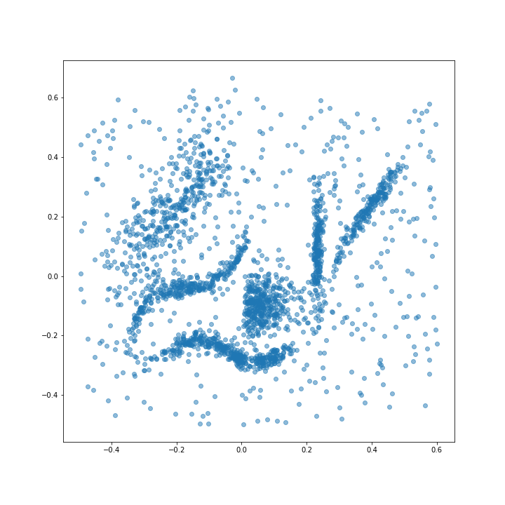
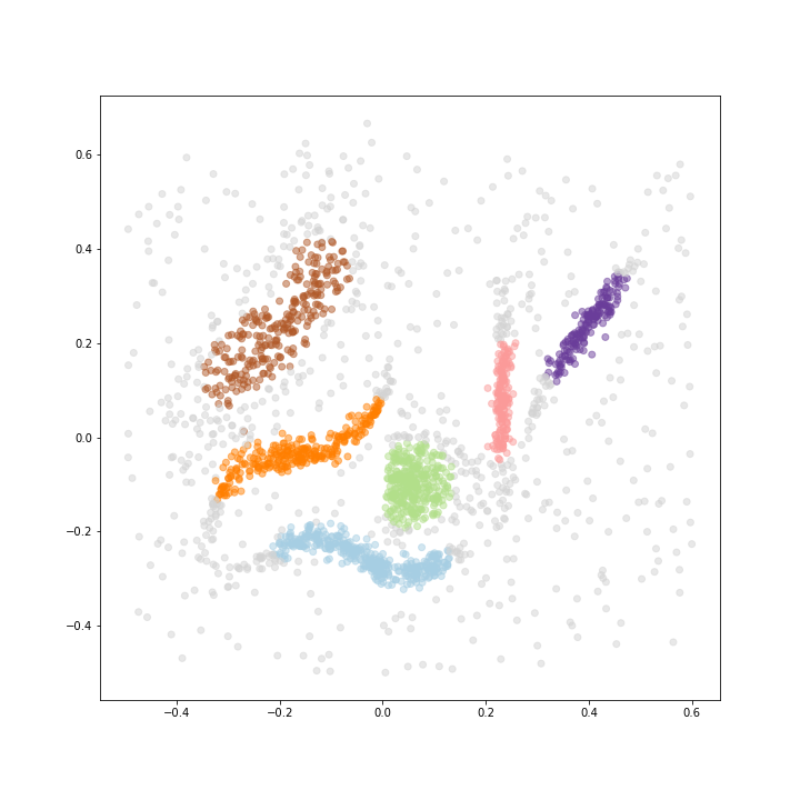
Figure 8: The running example. We cluster the data with Persistable: clusters are indicated by colors, and gray points are classified as noise.

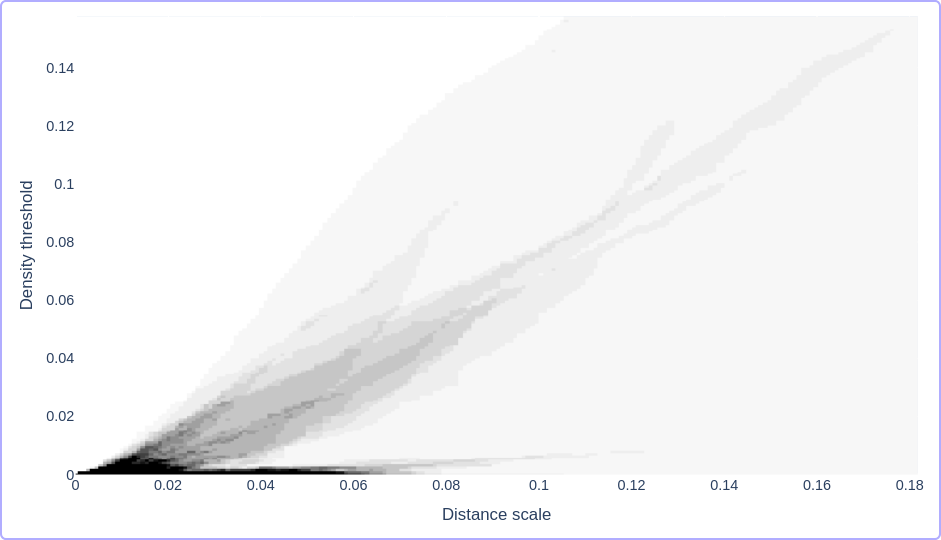
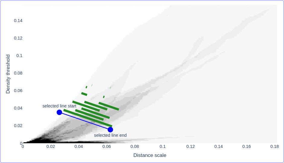
Figure 9: The first Persistable visualization is the component counting function; we show this for the running example. One can see typical behavior of degree-Rips ($\mathrm{DR}$): when the distance scale $s$ is small and the density threshold $k$ is large, no points are clustered; when $s$ is large and $k$ is small, all points are clustered together. In between these two regimes is a band of interesting cluster structure. The blue line segment defines a slice of $\mathrm{DR}$, and its barcode is plotted in green. The sixth gap size of this slice is quite large (the sixth-longest bar is much longer than the seventh-longest bar). So, we choose six clusters for the persistence-based flattening. The output is displayed in Fig. 8.

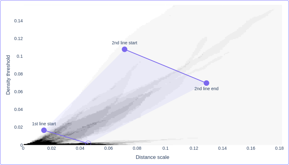
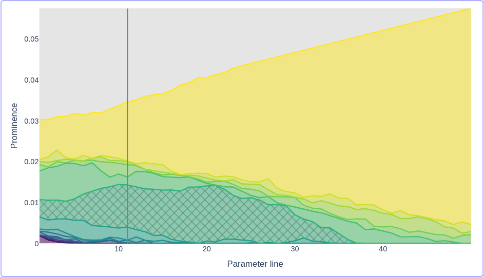
Figure 10: The second Persistable visualization is the prominence vineyard. The user chooses two slices of degree-Rips by choosing the start and end points. This determines a one-parameter family of slices that interpolate between the two chosen slices. For each slice in the family, Persistable computes the barcode, and the prominence vineyard (on the right) displays the prominence (i.e., length) of each bar in the barcode. So, the first (top) curve in the prominence vineyard shows the length of the longest bar in the barcode of each slice, the second curve shows the length of the second-longest bar, etc. We call these curves vines. The first gap (between the first and second vines, displayed in yellow) is very large: this just reflects the fact that the longest bar of an HC is typically much longer than any other bar. The sixth gap (marked in the figure) is also large. This means there are many slices in the vineyard such that the sixth gap size of the slice is large. We used this prominence vineyard to choose the slice in Fig. 9.

As input, Persistable takes a finite metric space $M$, and produces a clustering of $M$, in the sense of Definition . As a running example, we use a synthetic dataset from the hdbscan clustering library (McInnes et al., 2017). This dataset is designed to be challenging for clustering algorithms, while being easy to visualize: see Fig. 8.

Conceptually, Persistable begins with the degree-Rips hierarchical clustering $\mathrm{DR}(M)$ that was described in the introduction (see Fig. 1, and see Definition  for the formal definition). We can get insight into $\mathrm{DR}(M)$ by plotting the component counting function, which is the function defined on the first quadrant of the plane where at $(s,k)$ we simply count the number of clusters in $\mathrm{DR}(M)(s,k)$. The first visualization in the Persistable pipeline is a heat map of the component counting function. See Fig. 9 for this visualization on the running example.

Now, Persistable constructs a clustering of the input $M$ in two steps.

Step 1

Reduce from the two-parameter hierarchical clustering $\mathrm{DR}(M)$ to a one-parameter hierarchical clustering, by taking a slice (see Fig. 2). Using the notation established in Example , this means taking $\lambda\textup{-{link}}(M)$, where $\lambda$ is a choice of line in the $(s,k)$-parameter space. For example, see the blue line segment in Fig. 9. The practitioner can choose such a slice by clicking on the component counting visualization to choose the start and end points of a line segment. This determines an interval $(s_{\mathrm{start}},s_{\mathrm{end}})$ on which the one-parameter hierarchical clustering $\lambda\textup{-{link}}(M)$ is defined, and for $s\in(s_{\mathrm{start}},s_{\mathrm{end}})$, $\lambda\textup{-{link}}(M)(s)=\mathrm{DR}(M)(s,\sigma\cdot s+y)$, where $y$ is the $y$-intercept of the selected line, and $\sigma$ is its slope.

The second visualization in the Persistable pipeline is an interactive tool for choosing slices. We introduce this tool after we discuss the second step of Persistable.

Step 2

Reduce from the one-parameter hierarchical clustering $\lambda\textup{-{link}}(M)$ to a clustering of $M$, by applying the persistence-based flattening procedure, defined in Section 6. To apply the persistence-based flattening, one chooses the number of clusters in the output, guided by the barcode of the HC. The barcode is a visual summary of an HC (see Fig. 5). If one chooses $n$ clusters, these will correspond to the $n$ longest bars in the barcode. We call the difference between the length of the $n^{\mathrm{th}}$ longest and $(n+1)^{\mathrm{th}}$ longest bars the $n^{\mathrm{th}}$ gap size of the HC. As explained in Section 6, the larger the $n^{\mathrm{th}}$ gap size, the more stable the output with $n$ clusters will be. So, choosing the number of clusters boils down to looking at the barcode, and finding choices of $n$ such that the $n^{\mathrm{th}}$ gap size is large.

In the case of the running example, there is a drop-off between the sixth and seventh longest bars, so choosing six bars (i.e., six clusters) is a reasonable choice (see Fig. 9). The resulting clustering of the data is displayed in Fig. 8.

Choosing the slice

To complete the description of the Persistable pipeline, it remains to discuss how the practitioner chooses a slice. The answer is motivated by Step 2. When one applies the persistence-based flattening, one looks for large gap sizes in the barcode of $\lambda\textup{-{link}}(M)$. So, the second visualization tool in the Persistable pipeline helps the user identify slices $\lambda$ that lead to barcodes with large gap sizes.

The practitioner begins with the component counting visualization (Fig. 9). From this, one can find the region of the $\mathrm{DR}$ parameter space where interesting cluster structure is captured. The practitioner is asked to choose two slices in the $\mathrm{DR}$ parameter space, which determine a one-parameter family of slices that interpolate between the two chosen slices. As $\lambda$ varies in the family, the slice $\lambda\textup{-{link}}(M)$ changes in a continuous way by Proposition . Thus, the barcode of $\lambda\textup{-{link}}(M)$ also changes in a continuous way. In the prominence vineyard visualization, Persistable plots the prominence (i.e., length) of each bar in the barcode of $\lambda\textup{-{link}}(M)$. As $\lambda$ varies, these prominences trace out curves, which we call vines (this is standard terminology in topological data analysis, beginning with Cohen-Steiner et al., 2006). See Fig. 3. In Fig. 10, we display a prominence vineyard for the running example. There is a large gap between the first and second vines; this is typical behavior, as the longest bar in the barcode of an HC is just the interval on which the HC is non-empty, which is often much longer than any other bar. More interesting structure is captured by the other gaps in the prominence vineyard. For example, there is a large gap between the sixth and seventh vines, which is marked in Fig. 10. If we choose a slice that includes this gap, then the sixth gap size of the barcode of this slice is large. Indeed, this is how we picked the slice that we used in Step 2, above.

7.2 Examples of Persistable on benchmark datasets

Rideshare data

We consider a dataset consisting of approximately 560 000 rideshare pickup locations in the New York City area from April, 2014. The dataset is the result of a Freedom of Information request by the website FiveThirtyEight (2015). This dataset has very complex cluster structure, at many different scales. There are informative clusterings at a very coarse level, and also at much finer levels.

To get a feel for the data, we begin by considering the subset of points in a square centered at LaGuardia Airport (see Fig. 11), which consists of approximately 10 000 points.

\begin{overpic}[width=212.47617pt]{figures/laguardia-data.png} \put(52.0,49.0){{\footnotesize M}} \put(52.0,40.0){{\footnotesize H}} \put(60.0,32.0){{\footnotesize P}} \put(33.0,17.0){{\footnotesize S}} \put(83.0,55.0){{\footnotesize C}} \put(8.0,45.0){{\footnotesize A}} \put(11.0,55.0){{\footnotesize N}} \put(28.0,80.0){{\footnotesize B}} \end{overpic}

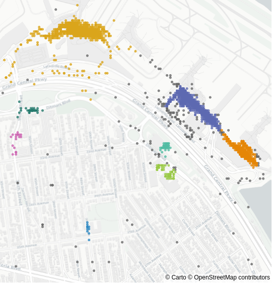
Figure 11: The subset of the Rideshare data in a square centered at LaGuardia Airport. On the left, some relevant landmarks are marked: ACE Rent A Car (A), National Car Rental (N), LaGuardia Airport Terminal B (B), Terminal C (C), Marriott Hotel (M), Hampton Inn Hotel (H), LaGuardia Plaza Hotel (P), P.S. 127 Aerospace Science Magnet School (S). On the right, a clustering produced by Persistable, using the slice displayed in Fig. 12. Gray points are unclustered.

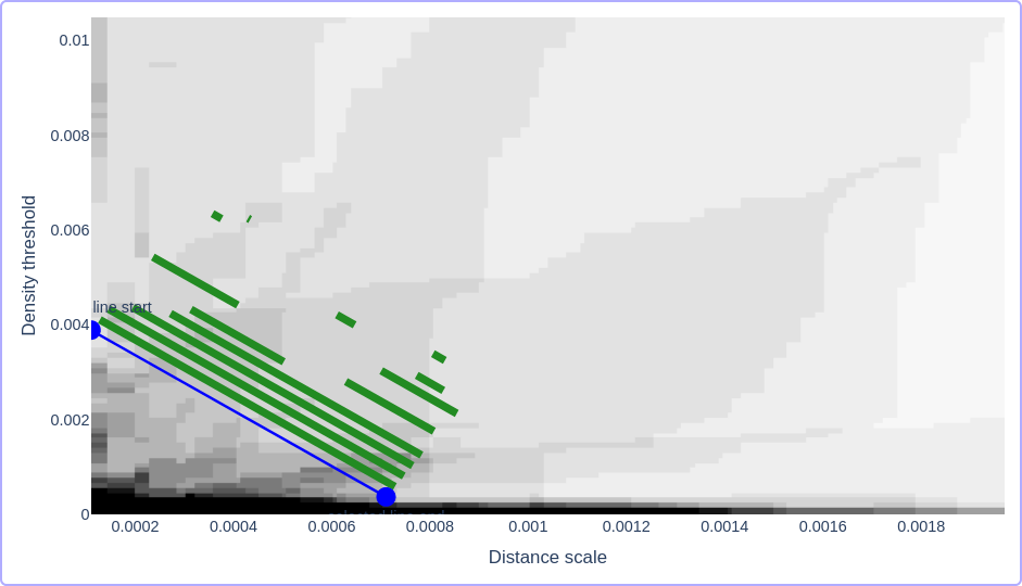
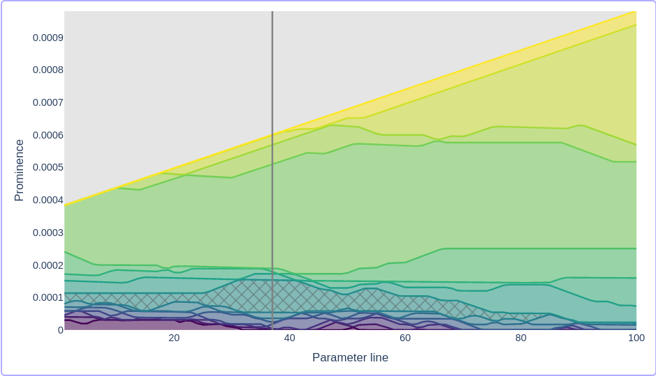
Figure 12: Persistable visualizations for the subset of the Rideshare data near LaGuardia Airport. On the left, the component counting visualization, and on the right, a prominence vineyard visualization. We use the prominence vineyard to choose a slice, which appears as the blue line segment on the component counting visualization; the corresponding slice in the vineyard is marked by a vertical line. The barcode of this slice is displayed in green. Several gaps in this vineyard lead to interesting clusterings. If we choose the gap below the eighth vine (marked in this figure), we get the clustering of the data displayed in Fig. 11. See Fig. 16 in Section A.6 for the result of choosing the gap below the fourth vine.

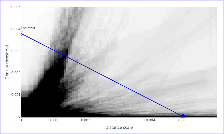
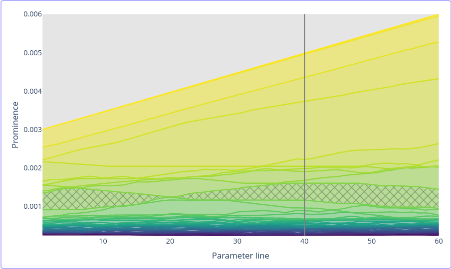
Figure 13: Persistable visualizations for the Rideshare data. On the left, the component counting visualization, and on the right, a prominence vineyard visualization. While the component counting visualization is very complicated, one can easily identify interesting gaps in the prominence vineyard. We use the prominence vineyard to choose a slice, marked on the component counting function by a blue line and on the vineyard by a vertical line. If we choose the marked gap, we get the clustering of the data displayed in Fig. 14.

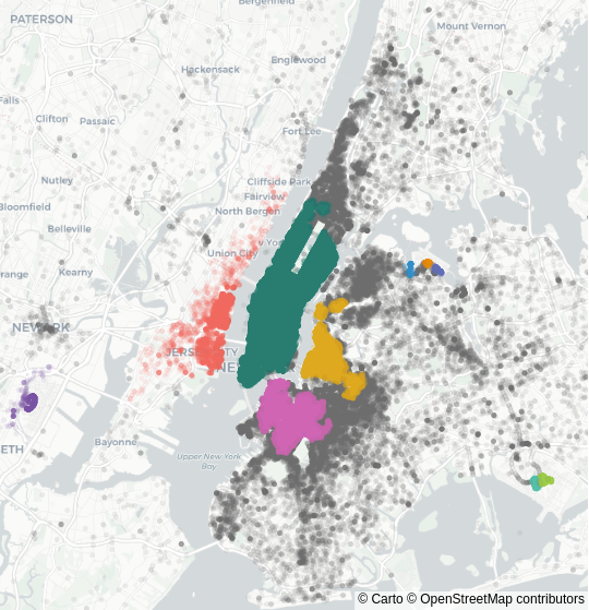
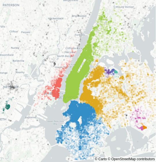
Figure 14: The Rideshare data, clustered using Persistable. Gray points are unclustered. In both cases, the clustering is obtained by choosing the slice indicated in Fig. 13. On the left, the clustering is obtained using the usual Persistable pipeline, choosing the gap marked in Fig. 13. On the right, the clustering is obtained using ExhaustivePF, rather than $\mathsf{PF}$. We find large clusters in Manhattan, Brooklyn, Queens, and New Jersey, as well as smaller clusters at Newark, LaGuardia, and John F. Kennedy airports.

While this dataset is easily visualizable, it is challenging for many density-based clustering algorithms, because its apparent cluster structure takes place at very different levels of density. For example, there are approximately 4000 data points clustered near Terminal B of the airport, and meanwhile, there is a cluster of approximately 60 data points near the LaGuardia Airport Marriott hotel, and an even smaller cluster of 12 data points near the P.S. 127 Aerospace Science Magnet School.

In particular, this dataset is challenging for HDBSCAN (Campello et al., 2013), a popular density-based clustering algorithm that is based on the robust single-linkage algorithm of Example  (for a description in these terms, see McInnes and Healy, 2018). Unlike the related DBSCAN algorithm (Ester et al., 1996), HDBSCAN can detect multi-scale cluster structure that takes place at a range of distance scales. However, like robust single-linkage, it relies on a fixed density threshold, and for this reason, cannot find the multi-scale cluster structure in this example (i.e., it cannot simultaneously find the large cluster near Terminal B and the small cluster near the hotel). See the jupyter notebook for this dataset at the Persistable repository (2023) to try clustering the data with HDBSCAN.

On the other hand, Persistable is sensitive to this kind of multi-scale clustering structure, because it uses slices of $\mathrm{DR}$ in which both the density threshold and the distance scale vary. In Fig. 12, we show Persistable visualizations for the data. Guided by these visualizations, one can use Persistable to find clusterings of the rideshare data that simultaneously capture the large clusters near the airport terminals and the small clusters in the surrounding neighborhood.

Now we consider the complete Rideshare dataset. The complexity of the data is reflected in the Persistable visualizations; see Fig. 13. Using Persistable, one can obtain informative clusterings of this data at coarser or finer scales. For example, see Fig. 14 for coarse but informative results. Using smaller gaps in the prominence vineyard, one can obtain finer results, with, for example, clusters centered at Penn Station and the Meatpacking district in Manhattan, and Williamsburg and Downtown Brooklyn. See the jupyter notebook for this dataset at the Persistable repository (2023) for details.

We are able to easily compute clusterings of this dataset with Persistable using the subsampling approximation described in Section 3.4 (which is justified by the Gromov–Hausdorff–Prokhorov stability of $\lambda$-linkage). Using a subsample of 30 000 data points, we are able to compute clusterings of the complete Rideshare dataset in a matter of seconds, using approximately 200 MB of RAM, using a laptop with an Intel(R) Core(TM) i5 CPU (4 cores, 1.6GHz) and 8 GB RAM, running GNU/Linux.

Without the subsampling approximation, clustering this dataset would be a significant computational challenge. For context, we clustered the data using the high-performance implementation of HDBSCAN of McInnes et al. (2017). This is a natural comparison, because HDBSCAN and Persistable are very similar on an algorithmic level, and because the implementation of McInnes et al. (2017) is very similar to our implementation of Persistable (indeed, important components of our implementation come directly from this implementation of HDBSCAN). The key performance advantage that Persistable has in this example is the subsampling approximation. An analogous approximation scheme is not valid for HDBSCAN, as the hierarchical clustering algorithm underlying HDBSCAN (robust single-linkage) is not Gromov–Hausdorff–Prokhorov stable (see Section 3.3).

See Table 1 in Section A.6 for the results. The memory usage of HDBSCAN scales with $n\cdot k$, where $n$ is the number of data points and $k$ is the density threshold parameter $\mathsf{min\_samples}$. This means that, on the laptop described above, we are only able to run HDBSCAN with very small values of the $\mathsf{min\_samples}$ parameter, producing only very fine clusterings.

Olive oil data

We consider a dataset concerning the fatty acid composition of $572$ samples of olive oil. For each sample, the percentages of $8$ fatty acids were measured. The samples were taken from nine regions of Italy, and these regions are grouped into three larger areas (South Italy, Sardinia, and North Italy). Each sample is labeled with its region of origin.

This is a useful test dataset for classification and clustering methods, and it is used as a benchmark dataset for density-based clustering by Stuetzle and Nugent (2010). The dataset is due to Forina et al. (1983), and we obtained it from the supplementary materials of Stuetzle and Nugent (2010). Using Persistable, one can recover much of the hierarchical clustering structure defined by the regions of origin.

We consider the data as points in $\mathbb{R}^{8}$ with the Euclidean metric; each feature is independently centered to have mean zero and scaled to unit variance. One can see many large gaps in the prominence vineyard visualization (see Fig. 15). This is a consequence of the multi-scale clustering structure of the data. For example, say we choose the slice indicated in Fig. 15. If we choose the large gap between the third and fourth vines (i.e., we choose three clusters in the persistence-based flattening), we get a clustering of the data that fits the large area labels perfectly, with $89\%$ of the data clustered (see Table 2 in Section A.6 for the confusion matrix). Meanwhile, if we choose the gap between the eighth and ninth vines marked in Fig. 15, we get a clustering that fits the region labels very accurately: the adjusted Rand index is $0.98$, and $49\%$ of the data is clustered (see Table 3 in Section A.6 for the confusion matrix).

In order to cluster more data points, we also run the exhaustive persistence-based flattening (Algorithm 2). We choose the same slice and gap as before, but replace the usual persistence-based flattening with the exhaustive persistence-based flattening. The result clusters $95\%$ of the data, with an adjusted Rand index of $0.90$ with respect to the region labels (see Table 4 in Section A.6 for the confusion matrix).

For comparison, Stuetzle and Nugent (2010) apply a density-based clustering algorithm to this data, and report an adjusted Rand index of $0.61$ with respect to the region labels, with all data points clustered.

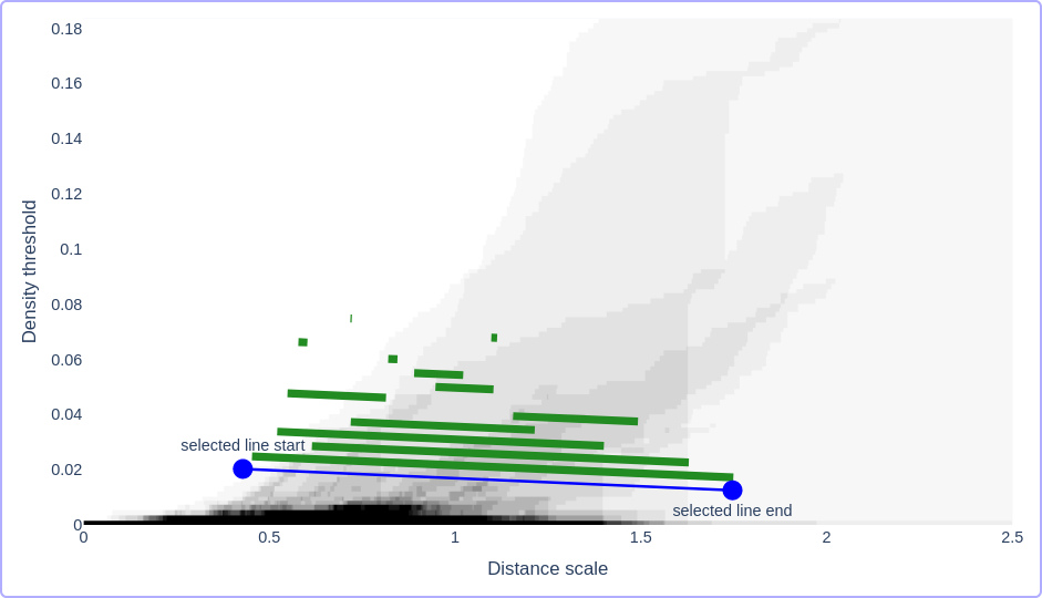
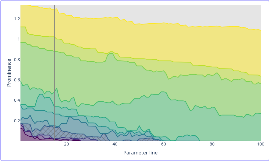
Figure 15: Persistable visualizations for the olive oil data. On the left, the component counting visualization, and on the right, a prominence vineyard visualization. We use the prominence vineyard to choose a slice, which appears as the blue line segment on the component counting visualization; the corresponding slice in the vineyard is marked by a vertical line. The barcode of this slice is displayed in green. Several gaps in this vineyard lead to interesting clusterings. If we choose the gap below the eighth vine (marked in this figure), we get a clustering that fits the region labels very accurately. If we choose the gap below the third vine, we get a clustering that fits the large area labels.

8 Conclusions

We conclude by mentioning some possible directions for future work. As we explained in Remark , Blumberg and Lesnick (2022) prove a stability result for the simplicial degree-Rips bifiltration using the Gromov–Prokhorov distance. The constant that appears in their result cannot be improved, but they give experimental evidence that a stronger stability result might be possible, and they pose the question of how to formulate such a result. The same question applies to the degree-Rips hierarchical clustering, and this setting might be a good place to start for this line of research.

In this paper we used slices of kernel linkage given by lines $\lambda$ in the parameter space. Our stability theorem for kernel linkage implies that appropriately chosen non-linear slices are also stable, and our consistency theorem applies also to appropriate non-linear slices. An interesting question is whether there are use cases in which non-linear slices lead to more informative clusterings.

For Persistable, we use a two-step process: we first reduce from degree-Rips to a one-parameter hierarchical clustering by taking a slice, then we reduce to a clustering using the persistence-based flattening. We do this because one-parameter hierarchical clusterings are much simpler than multiparameter hierarchical clusterings. See e.g. Bauer et al. (2020). In particular, the barcode and the persistence-based flattening algorithm are only defined for one-parameter hierarchical clusterings. Not much is known about flattening multiparameter hierarchical clusterings directly, but see Jardine (2019) and Shiebler (2021). An interesting question for future research is how one can stably extract a single clustering from degree-Rips or kernel linkage, without taking a one-parameter slice.

Acknowledgments

We thank Michael Lesnick for telling us about the good properties of one-parameter slices in which all parameters vary, and for telling us about his work with Blumberg on the stability of degree-Rips, which inspired our work here. We thank Leland McInnes for helpful discussion about HDBSCAN. And, we thank Dan Christensen, Rick Jardine, Michael Kerber, and Matt Piekenbrock for helpful discussions about this project and related topics.

L.S. was partially supported by the National Science Foundation through grants CCF-2006661 and CAREER award DMS-1943758.

A Missing details

A.1 Details from Section 2

Proof  (of Proposition ) First, say $H$ and $E$ are $\varepsilon$-interleaved for $\varepsilon\geq 0$. Let $x,y\in X$; we show $|\theta_{H}(x,y)-\theta_{E}(x,y)|\leq\varepsilon$. Without loss of generality, $\theta_{H}(x,y)\leq\theta_{E}(x,y)$. Let $r>\theta_{H}(x,y)$. Then there is $C\in\bar{H}(r)$ with $x,y\in C$. By the $\varepsilon$-interleaving property, there is $D\in\bar{E}(r+\varepsilon)$ with $C\subseteq D$, and thus $\theta_{E}(x,y)\leq r+\varepsilon$. This shows that $|\theta_{H}(x,y)-\theta_{E}(x,y)|\leq\varepsilon$, and it follows that $d_{\mathrm{I}}(H,E)\geq d_{\infty}(\theta_{H},\theta_{E})$.

Now, say $\varepsilon>d_{\infty}(\theta_{H},\theta_{E})$. We show $H$ and $E$ are $\varepsilon$-interleaved. Let $r\in\mathbb{R}$, and let $C\in\bar{H}(r)$. Choose $x\in C$. As $\theta_{H}(x,x)\leq r$, we have $\theta_{E}(x,x)<r+\varepsilon$, so that there is $D\in\bar{E}(r+\varepsilon)$ with $x\in D$. Similarly, for any $y\in C$, $\theta_{H}(x,y)\leq r$, so that $\theta_{E}(x,y)<r+\varepsilon$, and thus $y\in D$, and therefore $C\subseteq D$. This shows that $\bar{H}(r)\preceq\bar{E}(r+\varepsilon)$. A symmetric argument shows that $\bar{E}(r)\preceq\bar{H}(r+\varepsilon)$, and thus $H$ and $E$ are $\varepsilon$-interleaved. It follows that $d_{\mathrm{I}}(H,E)\leq d_{\infty}(\theta_{H},\theta_{E})$, and the proposition follows.  

Proof  (of Proposition ) Let $\varepsilon\geq 0$. We show that $||f-g||_{\infty}\leq\varepsilon$ if and only if $H(f)$ and $H(g)$ are $\varepsilon$-interleaved, and the proposition follows. If $||f-g||_{\infty}\leq\varepsilon$, then, for every $r\geq\varepsilon$, we have $\{f\geq r\}\subseteq\{g\geq r-\varepsilon\}$, and $\{g\geq r\}\subseteq\{f\geq r-\varepsilon\}$. This implies that, after taking connected components, every connected component of $\{f\geq r\}$ is included in a connected component of $\{g\geq r-\varepsilon\}$, and that every connected component of $\{g\geq r\}$ is included in a connected component of $\{f\geq r-\varepsilon\}$. If $H(f)$ and $H(g)$ are $\varepsilon$-interleaved, then, for every $x$ in the support of the functions, if $f(x)\geq\varepsilon$, then there exists a cluster in $\{g\geq f(x)-\varepsilon\}$ containing $x$, since $x\in\{f\geq f(x)\}$. This implies that for any $x$ in the support of the functions we have $g(x)\geq f(x)-\varepsilon$. A symmetric argument shows that $f(x)\geq g(x)-\varepsilon$ for every $x$ in the support, concluding the proof.  

Proof  (of Proposition ) The only non-trivial case is the triangle inequality, which is proved by composing correspondences. If $X,Y,Z$ are sets, and $R\subseteq X\times Y$ and $S\subseteq Y\times Z$ are correspondences, $S\circ R\subseteq X\times Z$ is the correspondence $S\circ R=\{(x,z):\exists y\in Y\text{ with }(x,y)\in R\text{ and }(y,z)\in S\}.$ If $H$ and $E$ are $\vec{\varepsilon}$-interleaved with respect to $R$, and $E$ and $F$ are $\vec{\delta}$-interleaved with respect to $S$, then $H$ and $F$ are $(\vec{\varepsilon}+\vec{\delta})$-interleaved with respect to $S\circ R$. From this it follows that $d_{\mathrm{CI}}(H,F)\leq d_{\mathrm{CI}}(H,E)+d_{\mathrm{CI}}(E,F)$.  

Lemma 0

Let $H$ and $E$ be ultrametric hierarchical clusterings of sets $X$ and $Y$ respectively. If $R$ is a correspondence between $X$ and $Y$, then the distortion of $R$ is $\mathrm{dis}(R)=\inf\{\varepsilon\geq 0:H,E\text{ are }\varepsilon\text{-interleaved w.r.t. }R\}$.

Proof  First we show that if $H$ and $E$ are $\varepsilon$-interleaved with respect to $R$, then $\mathrm{dis}(R)\leq\varepsilon$. Let $(x,y),(x^{\prime},y^{\prime})\in R$. If $r>\theta_{H}(x,x^{\prime})$, then there is $C\in\bar{H}(r)$ containing $x,x^{\prime}$, and thus $\pi_{X}^{-1}(C)$ contains $(x,y),(x^{\prime},y^{\prime})$. By the interleaving property, there is a cluster in $\pi_{Y}^{*}(\bar{E})(r+\varepsilon)$ containing $(x,y),(x^{\prime},y^{\prime})$, and thus there is a cluster in $\bar{E}(r+\varepsilon)$ containing $y,y^{\prime}$. So, $\theta_{E}(y,y^{\prime})\leq r+\varepsilon$, and thus $\theta_{E}(y,y^{\prime})\leq\theta_{H}(x,x^{\prime})+\varepsilon$. Together with a symmetric argument, we have $|\theta_{H}(x,x^{\prime})-\theta_{E}(y,y^{\prime})|\leq\varepsilon$. Thus $\mathrm{dis}(R)\leq\varepsilon$. Now, we show that $H$ and $E$ are $\varepsilon$-interleaved with respect to $R$, for any $\varepsilon>\mathrm{dis}(R)$, which finishes the proof. Let $r\in\mathbb{R}$ and let $C\in\bar{H}(r)$. We need to show there is $D\in\bar{E}(r+\varepsilon)$ such that $\pi_{X}^{-1}(C)\subseteq\pi_{Y}^{-1}(D)$. Let $x,x^{\prime}\in C$ and let $(x,y),(x^{\prime},y^{\prime})\in R$. We have $r\geq\theta_{H}(x,x^{\prime})$, therefore $\theta_{E}(y,y^{\prime})\leq r+\mathrm{dis}(R)$, and thus there is $D\in\bar{E}(r+\varepsilon)$ with $y,y^{\prime}\in D$. It follows that $(x,y),(x^{\prime},y^{\prime})\in\pi_{Y}^{-1}(D)$, and as $x,x^{\prime}$ were arbitrary, we have $\pi_{X}^{-1}(C)\subseteq\pi_{Y}^{-1}(D)$.  

Lemma 0

Let $K$ be a kernel, and let $\mathcal{M}$ be a metric probability space. Let $K^{-1}:\mathbb{R}_{>0}\rightarrow\mathbb{R}_{\geq 0}$ be defined as $K^{-1}(t)=\min\{u:K(u)\leq t\}$. Then $K^{-1}$ is a non-increasing function with compact support, and we have, for every $x\in\mathcal{M}$,

$$\left(\mu_{\mathcal{M}}\ast K_{s}\right)(x)=\int_{0}^{\infty}\mu_{\mathcal{M}}\left(B(x,sK^{-1}(r))\right)\,\,\mathsf{d}r.$$

Proof  Since $K(r)\rightarrow 0$ as $r\rightarrow\infty$, for every $t>0$ the set $\{u:K(u)\leq t\}$ is non-empty. Moreover, $K$ is continuous from the right, so the set has a minimum, and thus $K^{-1}$ is well-defined. The fact that $K^{-1}$ is non-increasing is clear, and the fact that it has compact support follows from the fact that $K$ is bounded.

To prove the statement about $\left(\mu_{\mathcal{M}}\ast K_{s}\right)$, we need the following straightforward fact about $K^{-1}$: for every $s,t\in\mathbb{R}_{\geq 0}$ we have $K^{-1}(t)>s$ if and only if $t<K(s)$. We finish the proof by computing

$$\int_{x^{\prime}\in\mathcal{M}}K\left(\frac{d(x,x^{\prime})}{s}\right)\,\mathsf{d}\mu_{\mathcal{M}} =\int_{x^{\prime}\in\mathcal{M}}\int_{0}^{\infty}\mathbf{1}_{\left\{r<K\left(\frac{d(x,x^{\prime})}{s}\right)\right\}}\,\mathsf{d}r\,\,\mathsf{d}\mu_{\mathcal{M}}$$

$$=\int_{x^{\prime}\in\mathcal{M}}\int_{0}^{\infty}\mathbf{1}_{\left\{d(x,x^{\prime})<sK^{-1}(r)\right\}}\,\mathsf{d}r\,\,\mathsf{d}\mu_{\mathcal{M}} =\int_{0}^{\infty}\int_{x^{\prime}\in\mathcal{M}}\mathbf{1}_{\left\{d(x,x^{\prime})<sK^{-1}(r)\right\}}\,\mathsf{d}\mu_{\mathcal{M}}\,\,\mathsf{d}r$$

$$=\int_{0}^{\infty}\mu_{\mathcal{M}}\left(B(x,sK^{-1}(r)\right)\,\mathsf{d}r,$$

as required.  

A.2 Details from Section 3

Lemma 0

Let $K$ be a kernel and let $r^{\prime}\in(0,K(0))$. Let $Z$ be a compact metric space and let $\mu$ and $\nu$ be Borel probability measures on $Z$ such that $d_{\mathrm{P}}(\mu,\nu)<\varepsilon$ for $\varepsilon>0$. Let $x,y\in Z$ such that $d_{Z}(x,y)<\varepsilon^{\prime}$. Then, for all $s>0$, we have $\left(\mu\ast K_{s}\right)(x)\leq\left(\nu\ast K_{s+\varepsilon_{s}}\right)(y)+\varepsilon_{k}$, for $\varepsilon_{s}=\frac{\varepsilon+\varepsilon^{\prime}}{K^{-1}(r^{\prime})}$ and $\varepsilon_{k}=K(0)\left(\frac{K(0)}{r^{\prime}}-1\right)+K(0)\varepsilon$.

Proof  Using Lemma , we know that $\left(\mu\ast K_{s}\right)(x)=\int_{0}^{K(0)}\mu(B(x,sK^{-1}(r)))\,\,\mathsf{d}r$, since, if $r>K(0)$, then $K^{-1}(r)=0$. Note that, for any radius $R\geq 0$, we have

$$\mu\left(B(x,R)\right)\leq\nu\left(B(x,R)^{\varepsilon}\right)+\varepsilon\leq\nu\left(B(x,R+\varepsilon)\right)+\varepsilon\leq\nu\left(B(y,R+\varepsilon+\varepsilon^{\prime})\right)+\varepsilon,$$

so we can bound the local density estimate of $x$ as follows:

$$\left(\mu\ast K_{s}\right)(x)\leq\int_{0}^{K(0)}\nu(B(y,sK^{-1}(r)+\varepsilon+\varepsilon^{\prime}))+\varepsilon\,\,\mathsf{d}r=\int_{0}^{K(0)}\nu(B(y,sK^{-1}(r)+\varepsilon+\varepsilon^{\prime}))\,\,\mathsf{d}r+K(0)\varepsilon.$$

Since $K^{-1}$ is non-increasing, and $r^{\prime}<K(0)$, it follows that $K^{-1}(rr^{\prime}/K(0))\geq K^{-1}(r)$ for every $r\geq 0$. Moreover, for any $0\leq r\leq K(0)$, we have $K^{-1}(rr^{\prime}/K(0))\geq K^{-1}(r^{\prime})$. These two considerations imply that, for $0\leq r\leq K(0)$, we have

$$sK^{-1}(r)+\varepsilon+\varepsilon^{\prime}\leq\left(s+(\varepsilon+\varepsilon^{\prime})/K^{-1}(r^{\prime})\right)K^{-1}\left(rr^{\prime}/K(0)\right).$$

Combining this with the above bound for the local density estimate of $x$ we get

$$\left(\mu\ast K_{s}\right)(x) \leq\int_{0}^{K(0)}\nu\left(B\left(y,\left(s+(\varepsilon+\varepsilon^{\prime})/K^{-1}(r^{\prime})\right)K^{-1}\left(rr^{\prime}/K(0)\right)\right)\right)\,\,\mathsf{d}r+K(0)\varepsilon$$

$$=\frac{K(0)}{r^{\prime}}\int_{0}^{r^{\prime}}\nu\left(B\left(y,\left(s+(\varepsilon+\varepsilon^{\prime})/K^{-1}(r^{\prime})\right)K^{-1}\left(r\right)\right)\right)\,\,\mathsf{d}r+K(0)\varepsilon$$

$$\leq\frac{K(0)}{r^{\prime}}\,\,\left(\nu\ast K_{\left(s+(\varepsilon+\varepsilon^{\prime})/K^{-1}(r^{\prime})\right)}\right)(y)+K(0)\varepsilon.$$

Finally, note that, for $0\leq a\leq M<\infty$ and $c\geq 1$, we have $ca\leq a+M(c-1)$. As $\nu$ is a probability measure, any local density estimate is bounded by $K(0)$. This implies that

$$\left(\mu\ast K_{s}\right)(x)\leq\left(\nu\ast K_{\left(s+(\varepsilon+\varepsilon^{\prime})/K^{-1}(r^{\prime})\right)}\right)(y)+K(0)\left(\frac{K(0)}{r^{\prime}}-1\right)+K(0)\varepsilon,$$

as required.  

Proof  (of Proposition ) We will construct a finite metric space $M$ such that $\mathrm{RSL}_{\kappa,\alpha}$ is not continuous at $M$. For any $\delta>0$, we will show that there is a finite metric space $N$ with $d_{\mathrm{GHP}}(M,N)<\delta$ such that $d_{\mathrm{CI}}(\mathrm{RSL}_{\kappa,\alpha}(M),\mathrm{RSL}_{\kappa,\alpha}(N))>1/2$.

Let $M\subset\mathbb{R}$ be a subset with $0,1\in M$, and with $\kappa-2$ points in the interval $(-\frac{1}{10},0)$ and $\kappa-2$ points in the interval $(1,\frac{11}{10})$. For $\ell\geq 1$, let $M_{\ell}=M\cup\{x+\frac{1}{\ell}:x\in M\}$. We have $d_{\mathrm{GHP}}(M,M_{\ell})\leq\frac{1}{\ell}$ for all $\ell\geq 1$. It remains to show that $d_{\mathrm{CI}}(\mathrm{RSL}_{\kappa,\alpha}(M),\mathrm{RSL}_{\kappa,\alpha}(M_{\ell}))>1/2$ for all sufficiently large $\ell$. Note that $\mathrm{RSL}_{\kappa,\alpha}(M)(r)=\emptyset$ for $r<1$; however, for $\ell\geq 10$, $0$ is in a cluster of $\mathrm{RSL}_{\kappa,\alpha}(M_{\ell})(r)$ for any $r>1/10$. This finishes the proof.  

As we described in Section 3, one could also formalize robust single-linkage by taking the density threshold parameter to be a ratio $k\in(0,1)$, and then letting $\mathrm{RSL}_{k,\alpha}(M)=\mathrm{L}(M)^{\gamma}$ for the covariant curve $\gamma\colon(0,\infty)\rightarrow\mathbb{R}_{>0}^{\times 3}$ with $\gamma(r)=(r,\alpha r,k)$. This variant also fails to be continuous with respect to the Gromov–Hausdorff–Prokhorov distance:

Proposition 0

Let $k\in(0,1)$ be rational, and let $\alpha>0$. With respect to the Gromov–Hausdorff–Prokhorov distance and the correspondence-interleaving distance, $\mathrm{RSL}_{k,\alpha}$ is discontinuous.

Proof  Write $k=p/q$. Without loss of generality, we may assume $p\geq 2$. We will construct a finite metric space $M$ such that $\mathrm{RSL}_{k,\alpha}$ is not continuous at $M$. Let $M\subset\mathbb{R}$ be a subset with $0\in M$, with $|M\cap(-\frac{1}{10},0)|=p-1$ and with $1,2,\dots,q-p\in M$. For $n\geq 1$, let

$$M_{n}=\left(M\cup M+\frac{1}{n^{2}}\cup\dots\cup M+\frac{n-1}{n^{2}}\right)\setminus\left\{\frac{n-1}{n^{2}}\right\}\,,$$

where $M+a=\{x+a:x\in M\}$. The idea is that we replace each point of $M$ with $n$ points that are tightly grouped together, except $0$, which we replace with only $n-1$ points (hence we remove the point $\frac{n-1}{n^{2}}$). We have $d_{\mathrm{GHP}}(M,M_{n})\rightarrow 0$ as $n\rightarrow\infty$. We have $0$ in a cluster of $\mathrm{RSL}_{k,\alpha}(M)(r)$ for any $r>1/10$; however, for $n$ sufficiently large, $\mathrm{RSL}_{k,\alpha}(M_{n})(r)=\emptyset$ for any $r\leq 1/2$. This shows that $d_{\mathrm{CI}}(\mathrm{RSL}_{k,\alpha}(M),\mathrm{RSL}_{k,\alpha}(M_{n}))>4/10$ for sufficiently large $n$, finishing the proof.  

Proof  (of Proposition ) For simplicity, we assume $\kappa^{\prime}=\kappa+1$, but the construction can easily be extended to the general case. Let $M\subset\mathbb{R}$ consist of $\kappa$ points in the interval $(-1,0)$, as well as the point $D+2$. Let $x\in M\cap(-1,0)$. Then $x$ is in a cluster of $\mathrm{RSL}_{\kappa,\alpha}(M)(r)$ for any $r>1$, but $\mathrm{RSL}_{\kappa^{\prime},\alpha}(M)(r)=\emptyset$ for all $r\leq D+2$.  

We also have the analogue of Proposition  for the variant of robust single-linkage that takes a density threshold $k\in(0,1)$ instead of $\kappa$:

Proposition 0

Let $k,k^{\prime}\in(0,1)$ be rational with $k\neq k^{\prime}$, and let $\alpha>0$. For any $D>0$, there is a finite metric space $M$ such that $d_{\mathrm{CI}}(\mathrm{RSL}_{k,\alpha}(M),\mathrm{RSL}_{k^{\prime},\alpha}(M))>D$.

Proof  The construction of $M$ is similar to the proof of Proposition . Write $k=p/q$. Without loss of generality, we may assume $p\geq 2$, and $k<k^{\prime}$. Let $M\subset\mathbb{R}$ be a subset with $0\in M$, with $|M\cap(-\frac{1}{2},0)|=p-1$, and with $D+1,2(D+1),\dots,q-p(D+1)\in M$. If $s\geq 1/2$, then $0$ is in a cluster of $\mathrm{RSL}_{k,\alpha}(M)$. However, if $s<D+1$, then $\mathrm{RSL}_{k^{\prime},\alpha}(M)=\emptyset$, and the proposition follows.  

Proof  (of Proposition ) Let $M=\{0,t\}\subset\mathbb{R}$. Say $\mathrm{PI}$ is defined using the kernel $K$. Because we always use isotropic kernels, we have $\left(\mu_{M}\ast K_{s}\right)(0)=\left(\mu_{M}\ast K_{s}\right)(t)=:M$. So, $\mathrm{PI}_{s,t}(M)(r)=\emptyset$ if $r>M$ and $\mathrm{PI}_{s,t}(M)(r)=\{M\}$ if $r\leq M$. Now, for any $\varepsilon>0$, let $M_{\varepsilon}=\{0,t+\varepsilon\}$. For any correspondence $R$ between $M$ and $M_{\varepsilon}$, we have $\pi_{M}^{*}(\mathrm{PI}_{s,t}(M))(r)=\{R\}$ for $r\leq M$, but $\pi_{M_{\varepsilon}}^{*}(\mathrm{PI}_{s,t}(M_{\varepsilon}))(r)\neq\{R\}$ for any $r>0$. So, for any $0\leq\delta<M$, $\mathrm{PI}_{s,t}(M)$ and $\mathrm{PI}_{s,t}(M_{\varepsilon})$ are not $\delta$-interleaved with respect to $R$, and thus $d_{\mathrm{CI}}(\mathrm{PI}_{s,t}(M),\mathrm{PI}_{s,t}(M_{\varepsilon}))>\delta$. But, as $\varepsilon\rightarrow 0$, we have $d_{\mathrm{GHP}}(M,M_{\varepsilon})\rightarrow 0$.  

Proof  (of Proposition ) Say $\mathrm{PI}$ is defined using the kernel $K$. Let $s>0$ be arbitrary, let $t=\min_{x\neq x^{\prime}}d_{M}(x,x^{\prime})$, and let $x_{0},x_{1}\in M$ be such that $d_{M}(x_{0},x_{1})=t$. If $t^{\prime}<t$, then $\mathrm{PI}_{s,t^{\prime}}(M)(r)$ consists of singletons for all $r>0$, while $\mathrm{PI}_{s,t}(M)(r)$ has a cluster containing $x_{0}$ and $x_{1}$ for all $r\leq\min(\left(\mu_{M}\ast K_{s}\right)(x_{0}),\left(\mu_{M}\ast K_{s}\right)(x_{1}))$. So, $d_{\mathrm{CI}}(\mathrm{PI}_{s,t}(M),\mathrm{PI}_{s,t^{\prime}}(M))$ does not go to zero as $t^{\prime}\rightarrow t$ from below.  

A.3 Details from Section 4

In order to prove that CI-consistency implies Hartigan consistency, we need a lemma, which is similar to Chaudhuri and Dasgupta (2010, Lemma 14, Appendix: Consistency), except that we do not require super-level sets to have finitely many connected components.

Lemma 0

Let $f:\mathbb{R}^{d}\rightarrow\mathbb{R}$ be a continuous, compactly supported probability density function, let $r>0$ and $A\neq A^{\prime}\in H(f)(r)$. There exists $\varepsilon>0$ and $B,B^{\prime}\in H(f)(r-\varepsilon)$ with $B\neq B^{\prime}$ such that $A\subseteq B$ and $A^{\prime}\subseteq B^{\prime}$.

Proof  Say, towards a contradiction, that for all $n$ with $1/n<r$, there is $B_{n}\in H(f)(r-1/n)$ with $A\subset B_{n}$ and $A^{\prime}\subset B_{n}$. It is a standard fact that if $K_{1}\supseteq K_{2}\supseteq\cdots$ is a nested sequence of non-empty, compact, connected sets in Euclidean space, then the intersection $\cap_{i=1}^{\infty}K_{i}$ is connected (Császár, 1978, 10.1.23). So, the intersection $B=\cap B_{n}$ is connected. For all $b\in B$, we have $f(b)\geq r-1/n$ for all $n$ large enough, so we must have $f(b)\geq r$. As $B$ is contained in $\{f\geq r\}$ and $B$ is connected, $B$ must intersect only one connected component of $\{f\geq r\}$, but we have $A\subset B$ and $A^{\prime}\subset B$, a contradiction.  

Proof  (of Proposition ) Given $r>0$ and distinct elements $A$ and $A^{\prime}$ of $H(f)(r)$, we show that the probability of $A_{n}\cap A^{\prime}_{n}=\emptyset$ goes to $1$ as $n\rightarrow\infty$, where $A_{n}$ is the smallest cluster in $\mathbb{A}^{\theta_{n}}(X_{n})$ that contains $A\cap X_{n}$ and likewise for $A^{\prime}$, and the $\theta_{n}$ are the parameters whose existence is given by CI-consistency of $\mathbb{A}$.

From Lemma  it follows that there exists $\varepsilon>0$ and distinct elements $B,B^{\prime}\in H(f)(r-\varepsilon)$ such that $A\subseteq B$ and $A^{\prime}\subseteq B^{\prime}$. Let $\delta\in(0,1)$. By assumption, there exists $N$ such that, if $n\geq N$, then the probability that $\mathbb{A}^{\theta_{n}}(X_{n})$ and $H(f)$ are $\varepsilon/2$-interleaved with respect to the closest point correspondence $R_{c}\subseteq X_{n}\times\mathcal{S}(f)$ is greater than $1-\delta$. As $R_{c}$ contains the pairs $(x,x)$ for $x\in X_{n}$, if $\mathbb{A}^{\theta_{n}}(X_{n})$ and $H(f)$ are $\varepsilon/2$-interleaved with respect to $R_{c}$, then $\mathbb{A}^{\theta_{n}}(X_{n})$ and $i^{*}(H(f))$ are $\varepsilon/2$-interleaved as hierarchical clusterings of $X_{n}$, where $i:X_{n}\rightarrow\mathcal{S}(f)$ is the inclusion. It is therefore enough to show that if $\mathbb{A}^{\theta_{n}}(X_{n})$ and $i^{*}(H(f))$ are $\varepsilon/2$-interleaved, then $A_{n}\cap A^{\prime}_{n}=\emptyset$. Now, if $\mathbb{A}^{\theta_{n}}(X_{n})$ and $i^{*}(H(f)))$ are $\varepsilon/2$-interleaved, then there exist $C,C^{\prime}\in\mathbb{A}^{\theta_{n}}(X_{n})(r-\varepsilon/2)$ such that $A\cap X_{n}\subseteq C\subseteq B$ and $A^{\prime}\cap X_{n}\subseteq C^{\prime}\subseteq B^{\prime}$. As $A_{n}\subseteq C$ and $A^{\prime}_{n}\subseteq C^{\prime}$, and $B\cap B^{\prime}=\emptyset$, we have $A_{n}\cap A^{\prime}_{n}=\emptyset$.  

We now prove Theorem , the CI-consistency of $\overline{\lambda}\textup{-{link}}$. Because the argument works in greater generality, we actually prove this for any “admissible family” of curves (this is Theorem ). The curves $\{\lambda_{\mathrm{con}}^{x,y}\}_{x,y>0}$ from Theorem  will be an example of an admissible family. We will use the following curves in order to define slices of kernel linkage.

Definition 0

A slicing curve consists of an interval $I_{\gamma}=(0,\max_{\gamma})$ with $\max_{\gamma}\in(0,\infty]$, and an order-preserving function $\gamma=(\gamma_{s},\gamma_{t},\gamma_{k}):I_{\gamma}^{\mathrm{op}}\rightarrow\mathbb{R}_{>0}\times\mathbb{R}_{>0}\times\mathbb{R}_{>0}^{\mathrm{op}}$, which we assume is continuous when viewed as a map between subspaces of Euclidean space. For any slicing curve $\gamma$ and any metric probability space $\mathcal{M}$, we write $\gamma\textup{-{link}}(\mathcal{M})=\mathrm{L}(\mathcal{M})^{\gamma}$.

As in Definition , we have to re-parameterize slices of kernel linkage in order to interleave them with the density-contour hierarchical clustering. We do this as follows.

Definition 0

Let $K$ be a kernel, and let $\gamma$ be a slicing curve. For $s>0$, we write $v_{s}=\int_{\mathbb{R}^{d}}K(||x||/s)\,\mathsf{d}x$. Define an order-preserving function $\varphi:I_{\gamma}\rightarrow\mathbb{R}_{>0}$ by $\varphi(r)=\gamma_{k}(r)/v_{\gamma_{s}(r)}$. We say that $\gamma$ is covering if $\gamma_{s}$ and $\gamma_{k}$ are injective, $\gamma_{s}(r)\rightarrow 0$ as $r\rightarrow\max_{\gamma}$, and $\gamma_{k}(r)\rightarrow 0$ as $r\rightarrow 0$. If $\gamma$ is covering, then $\varphi$ is a bijection. In that case, we write $\overline{\gamma}=\gamma\circ\varphi^{-1}:\mathbb{R}_{>0}^{\mathrm{op}}\rightarrow\mathbb{R}_{>0}\times\mathbb{R}_{>0}\times\mathbb{R}_{>0}^{\mathrm{op}}$. If $\gamma$ is a slicing curve that is covering, then $\overline{\gamma}$ is also a slicing curve.

From now on, fix a continuous, compactly-supported density function $f:\mathbb{R}^{d}\rightarrow\mathbb{R}$ with support $\mathcal{S}(f)$.

Notation 0

For $s>0$, define $f_{s}:\mathcal{S}(f)\rightarrow\mathbb{R}$ by

$$f_{s}(x)=\int_{\mathbb{R}^{d}}K\left(\frac{||x-y||}{s}\right)f(y)\;\,\mathsf{d}y.$$

Note that $f_{s}(x)=\left(f\ast K_{s}\right)(x)=\left(\mu_{f}\ast K_{s}\right)(x)$. As $\mathcal{S}(f)$ is compact, the continuous function $f$ is uniformly continuous. An elementary consequence (see e.g. Folland, 2013, Theorem 8.14) is that $f_{s}/v_{s}$ approximates $f$ for small enough $s$:

Lemma 0

Given $\varepsilon>0$ there exists $\delta>0$ such that if $s<\delta$ then $||f_{s}/v_{s}-f||_{\infty}<\varepsilon$.

Notation 0

Let $I\subseteq\mathbb{R}_{>0}^{\mathrm{op}}$ be an interval, and let $H:I\rightarrow\mathsf{C}(X)$ be a contravariant hierarchical clustering of a set $X$. We write $0pt_{H}:X\rightarrow[0,\infty]$ for the function defined by $0pt_{H}(x)=\sup\{r\in I\;:\;\exists C\in H(r),x\in C\}$.

Notation 0

We write $\mathrm{L}(f)$ for the kernel linkage of the metric probability space $(\mathcal{S}(f),\mu_{f})$. For any slicing curve $\gamma$, we write $h^{\gamma}=0pt_{\mathrm{L}(f)^{\gamma}}$. If $\gamma$ is covering, we write $h^{\overline{\gamma}}=0pt_{\mathrm{L}(f)^{\overline{\gamma}}}$.

Lemma 0

Let $\gamma$ be a slicing curve that is covering. Then, for any $x\in\mathcal{S}(f)$, the quantity $h^{\gamma}(x)$ satisfies $f_{\gamma_{s}(h^{\gamma}(x))}(x)=\gamma_{k}(h^{\gamma}(x))$. And, there exists $r_{1}\in I_{\gamma}$ such that $h^{\gamma}(x)<r_{1}$ for every $x\in\mathcal{S}(f)$.

Proof  Note first that, for any $x\in\mathcal{S}(f)$, $h^{\gamma}(x)=\sup\,\{r\in I_{\gamma}:f_{\gamma_{s}(r)}(x)\geq\gamma_{k}(r)\}$. We begin the proof by showing the following: there is $r_{1}\in I_{\gamma}$ such that $\{x\in\mathcal{S}(f):f_{\gamma_{s}(r_{1})}(x)\geq\gamma_{k}(r_{1})\}=\emptyset$, and there is $r_{0}\in I_{\gamma}$ such that $\{x\in\mathcal{S}(f):f_{\gamma_{s}(r_{0})}(x)\geq\gamma_{k}(r_{0})\}=\mathcal{S}(f)$. For the existence of $r_{1}$, note that $f_{\gamma_{s}(r)}(x)\leq v_{\gamma_{s}(r)}\cdot\max(f)$ for all $x\in\mathcal{S}(f)$ and $r\in I_{\gamma}$. So $r_{1}$ exists, since, as $r\rightarrow\max_{\gamma}$, we have $v_{\gamma_{s}(r)}\cdot\max(f)\rightarrow 0$ while $\gamma_{k}(r)$ is increasing. For the existence of $r_{0}$ note that, for every $r\in I_{\gamma}$, the function $f_{\gamma_{s}(r)}(x)$ is continuous in $x$ and strictly positive for every $x\in\mathcal{S}(f)$, so we have $\min(f_{\gamma_{s}(r)}(x))>0$ for any $r\in I_{\gamma}$. So $r_{0}$ exists since, as $r\rightarrow 0$, we have $\gamma_{k}(r)\rightarrow 0$ while $\min(f_{\gamma_{s}(r)}(x))$ is increasing.

Now, the function $f_{\gamma_{s}(r)}(x)$ is decreasing and continuous in $r$, and $\gamma_{k}(r)$ is continuous and strictly increasing in $r$. Since $f_{\gamma_{s}(r_{0})}(x)\geq\gamma_{k}(r_{0})$ and $f_{\gamma_{s}(r_{1})}(x)<\gamma_{k}(r_{1})$, we have that $h^{\gamma}(x)$ is the unique number $r\in[r_{0},r_{1}]$ such that $f_{\gamma_{s}(r)}(x)=\gamma_{k}(r)$, as required.  

Lemma 0

Let $\varepsilon>0$, and let $\gamma$ be a slicing curve that is covering. There is $\delta>0$ such that, if $\gamma_{s}(r)<\delta$ for every $r\in I_{\gamma}$, then $||h^{\overline{\gamma}}-f||_{\infty}<\varepsilon$.

Proof  Using Lemma , let $\delta$ be such that if $s<\delta$, then, for all $x\in\mathcal{S}(f)$, we have $|f_{s}(x)/v_{s}-f(x)|<\varepsilon$. By definition of $\overline{\gamma}$, we have $h^{\overline{\gamma}}(x)=\varphi(h^{\gamma}(x))$. Using Lemma , this implies that, for all $x\in\mathcal{S}(f)$,

$$h^{\overline{\gamma}}(x)=\varphi(h^{\gamma}(x))=\frac{\gamma_{k}(h^{\gamma}(x))}{v_{\gamma_{s}(h^{\gamma}(x))}}=\frac{f_{\gamma_{s}(h^{\gamma}(x))}(x)}{v_{\gamma_{s}(h^{\gamma}(x))}},$$

So, if $\gamma_{s}(r)<\delta$ for every $r\in I_{\gamma}$, then $|h^{\overline{\gamma}}(x)-f(x)|<\varepsilon$ as $\gamma_{s}(h^{\gamma}(x))<\delta$.  

Now, let $T$ be a topological space, and let $\mathcal{U}=\{U_{i}\}_{i=1}^{n}$ be an open cover of $T$, with $U_{i}\neq\emptyset$ for all $i$. Consider the graph $G_{\mathcal{U}}$ with vertex set $\{1,\dots,n\}$, and with an edge $(i,j)$ if $U_{i}\cap U_{j}\neq\emptyset$.

Lemma 0

If $T$ is a connected topological space, and $\mathcal{U}=\{U_{i}\}_{i=1}^{n}$ is a finite open cover of $T$ with $U_{i}\neq\emptyset$ for all $i$, then the graph $G_{\mathcal{U}}$ is connected.

Proof  We use induction on $n$. We assume the statement for $n-1$, and prove it for $n$. If $U_{1}\cap U_{i}=\emptyset$ for all $1<i\leq n$, then we can write $T=U_{1}\sqcup(\cup_{i=2}^{n}U_{i})$, contradicting the assumption that $T$ is connected. So, we can choose $1<j\leq n$ such that $U_{1}\cap U_{j}\neq\emptyset$. Let $\mathcal{U}^{\prime}=\{U_{1}\cup U_{j},U_{2},\dots,\hat{U_{j}},\dots,U_{n}\}$, where $\hat{U_{j}}$ indicates that we remove $U_{j}$. Then $\mathcal{U}^{\prime}$ is an open cover of $T$ with $n-1$ elements, so by induction, $G_{\mathcal{U}^{\prime}}$ is connected. Now, $G_{\mathcal{U}^{\prime}}$ is obtained by contracting the edge $\{1,j\}$ of $G_{\mathcal{U}}$. Thus, $G_{\mathcal{U}}$ is connected.  

Lemma 0

Let $\varepsilon>0$ and let $\gamma$ be a slicing curve that is covering. There is $\delta>0$ such that, if $\gamma_{s}(r),\gamma_{t}(r)<\delta$ for every $r\in I_{\gamma}$, then $\mathrm{L}(f)^{\overline{\gamma}}$ and $H(f)$ are $\varepsilon$-interleaved.

Proof  Using the fact that $f$ is uniformly continuous, Lemma , and Lemma , choose $\delta>0$ such that, for all $x,y\in\mathbb{R}^{d}$, if $||x-y||<\delta$, then $|f(x)-f(y)|<\varepsilon/2$, and such that, if $\gamma_{s}(r)<\delta$ for all $r\in I_{\gamma}$, then $||h^{\overline{\gamma}}-f||_{\infty}<\varepsilon/2$, and such that, if $s<\delta$, then $||f_{s}/v_{s}-f||_{\infty}<\varepsilon/2$. Let $\gamma$ be a slicing curve that is covering, and such that $\gamma_{s}(r),\gamma_{t}(r)<\delta$ for every $r\in I_{\gamma}$. We show that we have $\mathrm{L}(f)^{\overline{\gamma}}(r)\preceq H(f)(r-\varepsilon)$ and $H(f)(r)\preceq\mathrm{L}(f)^{\overline{\gamma}}(r-\varepsilon)$ in $\mathsf{C}(\mathcal{S}(f))$ for all $r>\varepsilon$.

By Lemma , for any $x\in\mathcal{S}(f)$, if $x$ is contained in a cluster of $\mathrm{L}(f)^{\overline{\gamma}}(r)$, then $x$ is contained in a cluster of $H(f)(r-\varepsilon)$; and if $x$ is contained in a cluster of $H(f)(r)$, then $x$ is contained in a cluster of $\mathrm{L}(f)^{\overline{\gamma}}(r-\varepsilon)$. Next, say $x,y\in C\in\mathrm{L}(f)^{\overline{\gamma}}(r)$ for $r>\varepsilon$. We show that $x$ and $y$ belong to the same cluster of $H(f)(r-\varepsilon)$. Let $r_{0}=\varphi^{-1}(r)$, $s_{0}=\gamma_{s}(r_{0})$, $t_{0}=\gamma_{t}(r_{0})$, and $k_{0}=\gamma_{k}(r_{0})$. So, by the definition of $\varphi$, we have $r=k_{0}/v_{s_{0}}$. Note we have $t_{0},s_{0}<\delta$. As $x,y\in C$, there is a chain $x_{0},\dots,x_{n}\in\mathcal{S}(f)$ with $x=x_{0},y=x_{n}$, such that $f_{s_{0}}(x_{i})\geq k_{0}$ and $||x_{i}-x_{i+1}||\leq t_{0}$ for all $i$. Dividing by $v_{s_{0}}$, we have $f_{s_{0}}(x_{i})/v_{s_{0}}\geq k_{0}/v_{s_{0}}=r$. Let $0\leq i\leq n-1$, and let $\alpha_{i}:[0,1]\rightarrow\mathbb{R}^{d}$ parameterize the straight-line path from $x_{i}$ to $x_{i+1}$. Let $q\in[0,1]$. Because $||x_{i}-\alpha_{i}(q)||\leq t_{0}<\delta$, we have $|f(x_{i})-f(\alpha_{i}(q))|<\varepsilon/2$. As $s_{0}<\delta$, we have $|f_{s_{0}}(x_{i})/v_{s_{0}}-f(x_{i})|<\varepsilon/2$. So, we have $f(\alpha_{i}(q))>r-\varepsilon$. The concatenation of the $\alpha_{i}$ is therefore a path in $\mathcal{S}(f)$ from $x$ to $y$ such that $f(p)>r-\varepsilon$ for all points $p$ on the path. So, $x$ and $y$ belong to the same cluster of $H(f)(r-\varepsilon)$.

Finally, let $x,y\in C\in H(f)(r)$. We show that $x$ and $y$ belong to the same cluster of $\mathrm{L}(f)^{\overline{\gamma}}(r-\varepsilon)$ for $r>\varepsilon$. Write $t_{\varepsilon}=\gamma_{t}(\varphi^{-1}(r-\varepsilon))>0$; we will show that there is a $t_{\varepsilon}$-chain $(x=x_{0},\dots,x_{n}=y)\in C$. Let $\{P_{i}\}_{i\in I}$ be the set of path components of $C$. For each $i\in I$, let $P_{i}^{t_{\varepsilon}}=\cup_{a\in P_{i}}B_{C}(a,t_{\varepsilon})$. Then, $\{P_{i}^{t_{\varepsilon}}\}_{i\in I}$ is an open cover of $C$. Since $C$ is compact, there is a finite $J\subseteq I$ such that $\mathcal{U}=\{P_{i}^{t_{\varepsilon}}\}_{i\in J}$ is an open cover of $C$.

Now, say $i,j\in J$, and $P_{i}^{t_{\varepsilon}}\cap P_{j}^{t_{\varepsilon}}\neq\emptyset$. We show that for any $a\in P_{i}$ and any $b\in P_{j}$, there is a $t_{\varepsilon}$-chain in $C$ connecting $a$ and $b$. Choose $w\in P_{i}^{t_{\varepsilon}}\cap P_{j}^{t_{\varepsilon}}$; by definition, there is $w_{i}\in P_{i}$ and $w_{j}\in P_{j}$ such that $||w-w_{i}||<t_{\varepsilon}$, and $||w-w_{j}||<t_{\varepsilon}$. Then, there is a $t_{\varepsilon}$-chain in $P_{i}$ connecting $a$ to $w_{i}$, and a $t_{\varepsilon}$-chain in $P_{j}$ connecting $b$ to $w_{j}$, which together give a $t_{\varepsilon}$-chain in $C$ connecting $a$ and $b$. By Lemma , the graph $G_{\mathcal{U}}$ is connected. So, there is a $t_{\varepsilon}$-chain in $C$ connecting $x$ and $y$.  

Definition 0

A slicing curve $\gamma=(\gamma_{s},\gamma_{t},\gamma_{k}):I_{\gamma}\rightarrow\mathbb{R}_{>0}^{3}$ is non-singular in each component if it is continuously differentiable and the derivatives $\gamma_{s}^{\prime},\gamma_{t}^{\prime}$, and $\gamma_{k}^{\prime}$ never vanish.

Definition 0

We say that a family $\{\gamma^{\theta}\}_{\theta\in\Theta}$ of slicing curves is an admissible family if each $\gamma^{\theta}$ is covering and non-singular in each component, and if, for every $b>0$, there is $\theta\in\Theta$ such that for all $r\in I_{\gamma^{\theta}}$, we have $\gamma^{\theta}_{s}(r),\gamma^{\theta}_{t}(r)<b$.

Lemma 0

Let $\gamma$ be a slicing curve that is non-singular in each component. Let $H$ and $E$ be $\mathbb{R}_{>0}\times\mathbb{R}_{>0}\times\mathbb{R}_{>0}^{\mathrm{op}}$-hierarchical clusterings of sets $X$ and $Y$ respectively, and let $R\subseteq X\times Y$ be a correspondence. Assume there exists $r\in I_{\gamma}$ with $H^{\gamma}(r)=\emptyset$. For every $\varepsilon>0$ there is $\delta>0$ such that, if $H$ and $E$ are $(\delta,\delta,\delta)$-interleaved with respect to $R$, then $H^{\gamma}$ and $E^{\gamma}$ are $\varepsilon$-interleaved with respect to $R$.

Proof  Choose $r_{0}\in I_{\gamma}$ such that $H^{\gamma}(r_{0})=\emptyset$ and let $\varepsilon>0$. Without loss of generality, suppose that $\varepsilon<r_{0}$. Choose $r_{1},r_{2}\in I_{\gamma}$ such that $r_{0}<r_{1}<r_{2}<\max_{\gamma}$. Let $c=\min_{r\in[\varepsilon/3,r_{2}]}\left\{\min\left(|\gamma^{\prime}_{s}(r)|,|\gamma^{\prime}_{t}(r)|,\gamma^{\prime}_{k}(r)\right)\right\}>0$. Let $\delta=\min(c(r_{1}-r_{0}),c\varepsilon/3)$. We show that if $H$ and $E$ are $(\delta,\delta,\delta)$-interleaved w.r.t. $R$, then $H^{\gamma}$ and $E^{\gamma}$ are $\varepsilon$-interleaved w.r.t. $R$.

Let $H^{\gamma}_{\varepsilon/3}$ be the $I_{\gamma}$-hierarchical clustering of $X$ with $H^{\gamma}_{\varepsilon/3}(r)=H^{\gamma}(r)$ for $r\in I_{\gamma}$ with $r>\varepsilon/3$, and $H^{\gamma}_{\varepsilon/3}(r)=\{X\}$ else. Define $E^{\gamma}_{\varepsilon/3}$ in the same way. Since $H^{\gamma}_{\varepsilon/3}$ and $H^{\gamma}$ are $\varepsilon/3$-interleaved, and similarly for $E^{\gamma}$, it suffices to show that $H^{\gamma}_{\varepsilon/3}$ and $E^{\gamma}_{\varepsilon/3}$ are $\varepsilon/3$-interleaved w.r.t. $R$. We first show that $E^{\gamma}(r_{1})=\emptyset$. It follows that $E^{\gamma}(r)=H^{\gamma}(r)=\emptyset$ for all $r\geq r_{1}$. By the definition of $c$, we have $\gamma_{s}(r_{1})+c(r_{1}-r_{0})\leq\gamma_{s}(r_{0})$, $\gamma_{t}(r_{1})+c(r_{1}-r_{0})\leq\gamma_{t}(r_{0})$, and $\gamma_{k}(r_{1})-c(r_{1}-r_{0})\geq\gamma_{k}(r_{0})$. Using these equations, the $(\delta,\delta,\delta)$-interleaving between $H$ and $E$, and the assumption that $\delta\leq c(r_{1}-r_{0})$, we have $\pi_{Y}^{*}(E^{\gamma})(r_{1})\preceq\pi_{X}^{*}(H^{\gamma})(r_{0})=\emptyset$, and thus $E^{\gamma}(r_{1})=\emptyset$. Now, to show that $H^{\gamma}_{\varepsilon/3}$ and $E^{\gamma}_{\varepsilon/3}$ are $\varepsilon/3$-interleaved w.r.t. $R$, it suffices to show that, for $r\in(2\varepsilon/3,r_{1})$, we have $\pi_{X}^{*}(H^{\gamma}_{\varepsilon/3})(r)\preceq\pi_{Y}^{*}(E^{\gamma}_{\varepsilon/3})(r-\varepsilon/3)$, and $\pi_{Y}^{*}(E^{\gamma}_{\varepsilon/3})(r)\preceq\pi_{X}^{*}(H^{\gamma}_{\varepsilon/3})(r-\varepsilon/3)$. Again by the definition of $c$, we have $\gamma_{s}(r)+c(\varepsilon/3)\leq\gamma_{s}(r-\varepsilon/3)$, $\gamma_{t}(r)+c(\varepsilon/3)\leq\gamma_{t}(r-\varepsilon/3)$, and $\gamma_{k}(r)-c(\varepsilon/3)\geq\gamma_{k}(r-\varepsilon/3)$ for any $r\in(2\varepsilon/3,r_{2})$. Using these equations, the $(\delta,\delta,\delta)$-interleaving between $H$ and $E$, and the assumption that $\delta\leq c\varepsilon/3$, we obtain the desired relations.  

Lemma 0

Let $\{\gamma^{\theta}\}_{\theta\in\Theta}$ be an admissible family of slicing curves, and let $X_{n}$ be a sample of $f$. For every $\varepsilon>0$ there exist $\theta\in\Theta$ and $\delta>0$ such that, if $d_{\mathrm{P}}(\mu_{n},\mu_{f}),d_{\mathrm{H}}(X_{n},\mathcal{S}(f))<\delta$, then $\mathrm{L}(X_{n})^{\overline{\gamma^{\theta}}}$ and $H(f)$ are $\varepsilon$-interleaved with respect to the closest point correspondence $R_{c}\subseteq X_{n}\times\mathcal{S}(f)$.

Proof  By Lemma , and the fact that the family $\{\gamma^{\theta}\}_{\theta\in\Theta}$ is admissible, we can fix the parameter $\theta$ so that $H(f)$ and $\mathrm{L}(f)^{\overline{\gamma^{\theta}}}$ are $\varepsilon/2$-interleaved. It is then enough to show that we can choose $\delta>0$ such that, if $d_{\mathrm{P}}(\mu_{n},\mu_{f})<\delta$ and $d_{\mathrm{H}}(X_{n},\mathcal{S}(f))<\delta$, then $\mathrm{L}(f)^{\overline{\gamma^{\theta}}}$ and $\mathrm{L}(X_{n})^{\overline{\gamma^{\theta}}}$ are $\varepsilon/2$-interleaved with respect to $R_{c}$. To see that this can be done, note that the operation $\mathrm{L}(-)^{\overline{\gamma^{\theta}}}$ is the composite of $\mathrm{L}(-)$ and slicing by $\overline{\gamma^{\theta}}$, and apply Theorem  (note that the interleaving constructed in the proof is with respect to $R_{c}$) and Lemma , where the last result applies by Lemma , since $\overline{\gamma^{\theta}}$ is covering.  

Lemma 0

Let $(\mathcal{M},d,\mu)$ be a compact metric probability space with full support and let $X_{n}$ be an i.i.d. $n$-sample of $\mathcal{M}$, seen as a subspace of $\mathcal{M}$. Let $\varepsilon>0$. Then, the probability that $\max(d_{\mathrm{P}}(\mu_{n},\mu),d_{\mathrm{H}}^{\mathcal{M}}(X_{n},\mathcal{M}))>\varepsilon$ goes to $0$ as $n\rightarrow\infty$. Here $\mu_{n}$ is the empirical measure given by the sample $X_{n}$.

Proof  We show that $P(d_{\mathrm{H}}^{\mathcal{M}}(X_{n},\mathcal{M})>\varepsilon)\rightarrow 0$ as $n\rightarrow\infty$. Since $\mathcal{M}$ is compact, for any $\varepsilon>0$ we can cover $\mathcal{M}$ with finitely many $\varepsilon$-balls, all of which have positive measure, by assumption. This implies that the probability that there is a sample point inside of each of these goes to $1$ as $n$ goes to $\infty$. We conclude by showing that $P(d_{\mathrm{P}}(\mu_{n},\mu)>\varepsilon)\rightarrow 0$ as $n\rightarrow\infty$. This follows from the facts that i.i.d. samples of a separable metric space with the empirical measure converge weakly to the sampled space, in probability (Parthasarathy, 1972, Chapter II, Theorem 7.1), and that weak convergence implies convergence in the Prokhorov distance (Billingsley, 1999, Section 6).  

Theorem 0

Let $\{\gamma^{\theta}\}_{\theta\in\Theta}$ be an admissible family of slicing curves. The hierarchical clustering algorithm $\overline{\gamma}\textup{-{link}}$ with parameter space $\Theta$, defined using any kernel $K$, is CI-consistent with respect to any continuous, compactly supported probability density function $f:\mathbb{R}^{d}\rightarrow\mathbb{R}$.

Proof  The theorem follows from Lemma  and the fact that samples converge to the space being sampled, Lemma .  

A.4 Details from Section 5

Lemma 0

Let $I\subseteq\mathbb{R}$ be an interval, let $H$ be an $I$-hierarchical clustering, and let $\mathbf{C}<\mathbf{D}\in\mathsf{PC}(H)$. Then, there exists $\mathbf{E}\in\mathsf{PC}(H)$ such that $\mathbf{E}<\mathbf{D}$ and $\mathbf{C}$ and $\mathbf{E}$ are incomparable.

Proof  Let $r<s\in I$ and $C\in H(r)$ and $D\in H(s)$ such that $[C]=\mathbf{C}$ and $[D]=\mathbf{D}$. Since $\mathbf{C}\neq\mathbf{D}$, there must exist $t\in[r,s]$ and $E\in H(t)$ such that $E\subseteq D$ but $C\not\subseteq E$. Then, the persistent cluster $\mathbf{E}\in\mathsf{PC}(H)$ satisfies the required conditions.  

Lemma 0

Let $I\subseteq\mathbb{R}$ be an interval, $H$ be an $I$-hierarchical clustering, and let $\mathbf{C},\mathbf{D}\in\mathsf{PC}(H)$. If $U(\mathbf{C})\cap U(\mathbf{D})\neq\emptyset$, then $U(\mathbf{C})\subseteq U(\mathbf{D})$ or $U(\mathbf{D})\subseteq U(\mathbf{C})$. Moreover, if $U(\mathbf{C})=U(\mathbf{D})$, then $\mathbf{C}=\mathbf{D}\in\mathsf{PC}(H)$.

Proof  Say $U(\mathbf{C})\cap U(\mathbf{D})\neq\emptyset$, and let $x\in U(\mathbf{C})\cap U(\mathbf{D})$. Choose $r\in\mathsf{life}(\mathbf{C})$ with $x\in\mathbf{C}(r)$ and $r^{\prime}\in\mathsf{life}(\mathbf{D})$ with $x\in\mathbf{D}(r^{\prime})$. Without loss of generality, $r\leq r^{\prime}$, and thus $\mathbf{C}(r)\subseteq\mathbf{D}(r^{\prime})$. We show $U(\mathbf{C})\subseteq U(\mathbf{D})$. Say $y\in U(\mathbf{C})$. Choose $i\in\mathsf{life}(\mathbf{C})$ with $y\in\mathbf{C}(i)$. We may assume $i\geq r$. If $r^{\prime}\in\mathsf{life}(\mathbf{C})$, then $\mathbf{C}(r^{\prime})=\mathbf{D}(r^{\prime})$, and thus $\mathbf{C}=\mathbf{D}$. So, assume $r^{\prime}\not\in\mathsf{life}(\mathbf{C})$. As $\mathsf{life}(\mathbf{C})$ is an interval, $i<r^{\prime}$, and thus $\mathbf{C}(i)\subseteq\mathbf{D}(r^{\prime})$. So, $y\in\mathbf{D}(r^{\prime})\subseteq U(\mathbf{D})$.

Now, assume $U(\mathbf{C})=U(\mathbf{D})$. As in the first step above, we have without loss of generality $\mathbf{C}(r)\subseteq\mathbf{D}(r^{\prime})$ for some $r\leq r^{\prime}$. We show $\mathbf{C}(r)\sim\mathbf{D}(r^{\prime})$. Let $r^{\prime\prime}\in[r,r^{\prime}]$, and let $A,A^{\prime}\in H(r^{\prime\prime})$ with $A,A^{\prime}\subseteq\mathbf{D}(r^{\prime})$. We have $A,A^{\prime}\subseteq U(\mathbf{D})=U(\mathbf{C})$. Let $B\in H(r^{\prime\prime})$ be the cluster such that $\mathbf{C}(r)\subseteq B$. It is straightforward to show $A=B$, and similarly $A^{\prime}=B$. Thus $A=A^{\prime}$, finishing the proof.  

Lemma 0

Let $I\subseteq\mathbb{R}$ be an interval, let $H$ be an $I$-hierarchical clustering, and let $\mathbf{C}<\mathbf{D}\in\mathsf{PC}(H)$. Then, the set $\{\mathbf{D}\in\mathsf{PC}(H):\mathbf{D}\geq\mathbf{C}\}$ is linearly ordered in $\mathsf{PC}(H)$.

Proof  Let $r,r^{\prime}\in I$, $D\in H(r)$, $D^{\prime}\in H(r^{\prime})$ such that $[D]=\mathbf{D}$ and $[D^{\prime}]=\mathbf{D}^{\prime}$. Assume, without loss of generality, that $r\leq r^{\prime}$. Since $\mathbf{C}\leq\mathbf{D},\mathbf{D}^{\prime}$, we have $U(\mathbf{C})\subseteq D$ and $U(\mathbf{C})\subseteq D^{\prime}$. If follows that $U(\mathbf{D})\cap U(\mathbf{D}^{\prime})\neq\emptyset$ and thus $\mathbf{D}\leq\mathbf{D}^{\prime}$ or $\mathbf{D}^{\prime}\leq\mathbf{D}$, by Lemma .  

Definition 0

Let $H$ be a one-parameter hierarchical clustering and let $\mathbf{C}\in\mathsf{PC}(H)$. The successor of $\mathbf{C}$ is, if it exists, the unique minimal element of $\{\mathbf{D}\in\mathsf{PC}(H):\mathbf{D}>\mathbf{C}\}$, where uniqueness follows from the fact that $\{\mathbf{D}\in\mathsf{PC}(H):\mathbf{D}>\mathbf{C}\}$ is linearly ordered (Lemma ).

We now recall the terminology of persistence modules; we refer the interested reader to Chazal et al. (2016); Bauer and Lesnick (2015) for details. Fix a field $\mathbb{F}$. Let $I\subseteq\mathbb{R}$ be an interval, and let $H$ be an $I$-hierarchical clustering of a set $X$. For each $r\in I$, consider the vector space $\mathbb{F}H(r)$ that is freely generated by the clusters of $H(r)$. For $r\leq r^{\prime}$, there is a linear map $\mathbb{F}H(r)\rightarrow\mathbb{F}H(r^{\prime})$ defined on the basis given above by $H(r\leq r^{\prime})$. This data gives a functor $\mathbb{F}H:I\rightarrow\mathbb{F}\text{-}\mathbf{vec}$, where $\mathbb{F}\text{-}\mathbf{vec}$ is the category of vector spaces over $\mathbb{F}$. Analogously to Definition , we call such a functor an $I$-persistence module.

Let $I\subseteq\mathbb{R}$ be an interval and let $M:I\rightarrow\mathbb{F}\text{-}\mathbf{vec}$ be an $I$-persistence module. Given $r\leq r^{\prime}\in I$, define the rank invariant (Zomorodian and Carlsson, 2005) of $M$ at $r\leq r^{\prime}$ as $\mathrm{rk}(M)(r\leq r^{\prime})=\mathrm{rk}(M(r)\rightarrow M(r^{\prime}))$. Note that $\mathrm{rk}(H)=\mathrm{rk}(\mathbb{F}H)$.

For our purposes, given a set $A$, a multiset of elements of $A$ consists of an indexing set $J$ and a function $a:J\rightarrow A$. We usually denote such a multiset by $\{a_{j}\}_{j\in J}$. We say that two multisets $\{a_{j}\}_{j\in J}$ and $\{b_{k}\}_{k\in K}$ of elements of $A$ are equal if there exists a bijection $\beta:J\rightarrow K$ such that $a_{j}=b_{\beta(j)}$ for all $j\in J$.

Let $B\subseteq I\subseteq\mathbb{R}$ be inclusions of intervals. The $I$-persistence module $\mathbb{F}_{B}:I\rightarrow\mathbb{F}\text{-}\mathbf{vec}$ is the functor taking the value $\mathbb{F}$ on every $r\in B$ and the value $0$ elsewhere, with structure morphism being the identity $\mathbb{F}\rightarrow\mathbb{F}$ whenever that is possible. The following theorem is due to Crawley-Boevey.

Theorem 0 (cf. (Crawley-Boevey, 2015, Theorem 1.1))

Let $\mathbb{F}$ be a field, let $I\subseteq\mathbb{R}$ be an interval, and let $M:I\rightarrow\mathbb{F}\text{-}\mathbf{vec}$ be an $I$-persistence module. If $M$ is pointwise finite dimensional, then there exists a unique multiset of intervals $\{B_{j}\subseteq I\}_{j\in J}$ such that $M$ is isomorphic to $\bigoplus_{j\in J}\mathbb{F}_{B_{j}}$.

Lemma 0

Let $I\subseteq\mathbb{R}$ be an interval. Let $H$ be a pointwise finite $I$-hierarchical clustering and let $\mathbb{F}$ be any field. Then $\mathcal{B}(H)$ is the unique multiset $\{B_{j}\subseteq I\}_{j\in J}$ such that $\mathbb{F}H\cong\bigoplus_{j\in J}\mathbb{F}_{B_{j}}$.

Proof  By definition, the $I$-persistence module $\mathbb{F}H:I\rightarrow\mathbb{F}\text{-}\mathbf{vec}$ is pointwise finite dimensional, in the sense of Crawley-Boevey (2015). Thus, by Theorem , there exist a unique multiset of intervals $\{B_{j}\subseteq I\}_{j\in J}$ such that $\mathbb{F}H\cong\bigoplus_{j\in J}\mathbb{F}_{B_{j}}$. By unfolding definitions, we get

$$\mathrm{rk}\left(\bigoplus_{j\in J}\mathbb{F}_{B_{j}}\right)(r\leq r^{\prime})=\sum_{j\in J}\mathrm{rk}\left(\mathbb{F}_{B_{j}}\right)(r\leq r^{\prime})=|\{j\in J:r,r^{\prime}\in B_{j}\}|,$$

so $\{B_{j}\subseteq I\}_{j\in J}$ is a barcode for $H$.

The fact that the barcode is unique is a particular case of (Botnan et al., 2022, Proposition 2.8), where the poset $P$ is taken to be $I$ and the collections of intervals $\widehat{\mathcal{I}}$ and $\mathcal{I}$ are all intervals included in $I$.  

Proof  (of Theorem ) This follows at once from Theorem  and Lemma .  

Lemma 0

Let $H$ be a finite $I$-hierarchical clustering. Then

$$|\mathsf{leaves}(H)|=\max\{k\in\mathbb{N}:\exists\{r_{j}\in I\}_{1\leq j\leq k},\{D_{j}\in H(r_{j})\}_{1\leq j\leq k}\text{ s.t. }D_{i}\subseteq D_{j}\Rightarrow i=j\},$$

and any set $\{D_{j}\in H(r_{j})\}_{1\leq j\leq k}$ attaining the maximum must be such that $\{[D_{j}]\in\mathsf{PC}(H)\}=\mathsf{leaves}(H)$.

Proof  The inequality $(\leq)$ follows immediately by taking the set of clusters $\{D_{j}\}$ to be a set of representatives of the leaves of $H$. The inequality $(\geq)$ follows from the fact that, given a set $\{D_{j}\in H(r_{j})\}_{1\leq j\leq k}$ as in the statement, the set $\{[D_{j}]\in\mathsf{PC}(H)\}_{1\leq j\leq k}$ forms an antichain of $\mathsf{PC}(H)$ and thus its cardinality is bounded above by the cardinality of the set of minimal elements of $\mathsf{PC}(H)$, which is, by definition, the set of leaves. To prove the last claim, note that any antichain of $\mathsf{PC}(H)$ of cardinality $|\mathsf{leaves}(H)|$ must necessarily be the set $\mathsf{leaves}(H)$ itself, since $\mathsf{PC}(H)$ forms a forest.  

Lemma 0

Let $H$ be a finite $I$-hierarchical clustering of a set $X$. Assume that $H$ is not constantly empty and let $\mathbf{C}\in\mathsf{leaves}(H)$. Then

1. $H\setminus\mathbf{C}$ is a finite $I$-hierarchical clustering;

2. $|\mathsf{leaves}(H\setminus\mathbf{C})|=|\mathsf{leaves}(H)|-1$;

3. If $|\mathsf{leaves}(H)|\geq 2$, then $\min_{\mathbf{D}\in\mathsf{leaves}(H)}\mathsf{length}(\mathbf{D})\leq\min_{\mathbf{D}^{\prime}\in\mathsf{leaves}(H\setminus\mathbf{C})}\mathsf{length}(\mathbf{D}^{\prime})$.

Proof  Note first that if $D_{1}\in H(r_{1})$ and $D_{2}\in H(r_{2})$ are such that $[D_{1}]=[D_{2}]$ in $\mathsf{PC}(H)$ and $[D_{1}]\neq\mathbf{C}$, then $[D_{1}]=[D_{2}]$ in $\mathsf{PC}(H\setminus\mathbf{C})$. Using this fact, we can define a function $\varphi:\mathsf{PC}(H)\setminus\mathbf{C}\rightarrow\mathsf{PC}(H\setminus\mathbf{C})$ as follows. For $\mathbf{D}\in\mathsf{PC}(H)\setminus\mathbf{C}$, pick any $D\in\mathbf{D}$, and let $\varphi(\mathbf{D})=[D]\in\mathsf{PC}(H\setminus\mathbf{C})$. We now prove that $\varphi$ is surjective, which implies the first statement of the lemma. Let $\mathbf{D}\in\mathsf{PC}(H\setminus\mathbf{C})$, and let $D\in\mathbf{D}$. Then $[D]\neq\mathbf{C}$ in $\mathsf{PC}(H)$ by definition of $H\setminus\mathbf{C}$. So, $\varphi([D])=\mathbf{D}$.

Next, we show that, when $\varphi$ is restricted to $\mathsf{leaves}(H)\setminus\mathbf{C}$, $\varphi$ is a bijection between $\mathsf{leaves}(H)\setminus\mathbf{C}$ and $\mathsf{leaves}(H\setminus\mathbf{C})$; this proves the second statement of the lemma. For this, we will use the following fact, which is straightforward to check. If $G$ is an $I$-hierarchical clustering, and $\mathbf{A}\in\mathsf{PC}(G)$, then $\mathbf{A}$ is a leaf if and only if for any $r\in\mathsf{life}(\mathbf{A})$ and for any $r^{\prime}\in I$ with $r^{\prime}<r$, there is at most one cluster $B\in H(r^{\prime})$ with $B\subseteq\mathbf{A}(r)$. Now, let $\mathbf{D}\in\mathsf{leaves}(H)\setminus\mathbf{C}$. We need to show $\varphi(\mathbf{D})$ is a leaf. Let $D=\mathbf{D}(r)$ for some $r$, so that $\varphi(\mathbf{D})=[D]$. If there is $r^{\prime}<r$ and $B,B^{\prime}\in(H\setminus\mathbf{C})(r^{\prime})$ with $B,B^{\prime}\subseteq D$, then as $\mathbf{D}$ is a leaf of $H$, we have $B=B^{\prime}$. Let $s\in\mathsf{life}(\varphi(\mathbf{D}))$, and let $s^{\prime}\in I$ with $s^{\prime}<s$. If $s^{\prime}<r$, then we have shown that there is at most one cluster in $(H\setminus\mathbf{C})(s^{\prime})$ contained in $\varphi(\mathbf{D})(s)$. If $r\leq s^{\prime}$, then as $\varphi(\mathbf{D})(r)\sim\varphi(\mathbf{D})(s)$, there is exactly one cluster in $(H\setminus\mathbf{C})(s^{\prime})$ contained in $\varphi(\mathbf{D})(s)$. So, $\varphi(\mathbf{D})$ is a leaf.

We show that $\varphi|_{\mathsf{leaves}(H)\setminus\mathbf{C}}$ is injective. Say $\mathbf{D},\mathbf{E}\in\mathsf{leaves}(H)\setminus\mathbf{C}$ and $\mathbf{D}\neq\mathbf{E}$. Let $D=\mathbf{D}(r)$ and $E=\mathbf{E}(r^{\prime})$ for some $r,r^{\prime}$. As $\mathbf{D}$ and $\mathbf{E}$ are distinct leaves, Lemma  implies $D\cap E=\emptyset$. As $D=\varphi(\mathbf{D})(r)$ and $E=\varphi(\mathbf{E})(r^{\prime})$, we have $\varphi(\mathbf{D})\neq\varphi(\mathbf{E})$.

Next we show that the image of $\varphi|_{\mathsf{leaves}(H)\setminus\mathbf{C}}$ is $\mathsf{leaves}(H\setminus\mathbf{C})$. Say $\mathbf{D}\in\mathsf{leaves}(H\setminus\mathbf{C})$. Let $D=\mathbf{D}(r)$ for some $r$. If $[D]\in\mathsf{leaves}(H)$, then we are done, since $\varphi([D])=\mathbf{D}$. So, say $[D]$ is not a leaf of $H$. Then there is $r^{\prime}\in I$ with $r^{\prime}<r$ and $B,B^{\prime}\in H(r^{\prime})$ with $B\neq B^{\prime}$ and $B,B^{\prime}\subseteq D$. Without loss of generality, $B\not\in(H\setminus\mathbf{C})(r^{\prime})$, so $[B]=\mathbf{C}$ in $\mathsf{PC}(H)$. Thus, $[B^{\prime}]\neq\mathbf{C}$, so that $B^{\prime}\in(H\setminus\mathbf{C})(r^{\prime})$. As $\mathbf{D}$ is a leaf of $H\setminus\mathbf{C}$, we have $[B^{\prime}]=\mathbf{D}$ in $\mathsf{PC}(H\setminus\mathbf{C})$, so that $\varphi([B^{\prime}])=\mathbf{D}$. We show that $[B^{\prime}]\in\mathsf{leaves}(H)\setminus\mathbf{C}$. Say there is $r^{\prime\prime}<r^{\prime}$ and $A,A^{\prime}\in H(r^{\prime\prime})$ with $A,A^{\prime}\subseteq B^{\prime}$. Then $A\cap B=\emptyset$ and $A^{\prime}\cap B=\emptyset$, so that $[A]\neq\mathbf{C}$ and $[A^{\prime}]\neq\mathbf{C}$ in $\mathsf{PC}(H)$. Thus, $A,A^{\prime}\in(H\setminus\mathbf{C})(r^{\prime\prime})$, and since $\mathbf{D}$ is a leaf of $H\setminus\mathbf{C}$, $A=A^{\prime}$.

We have shown that $\varphi|_{\mathsf{leaves}(H)\setminus\mathbf{C}}$ is a bijection between $\mathsf{leaves}(H)\setminus\mathbf{C}$ and $\mathsf{leaves}(H\setminus\mathbf{C})$, proving the second statement of the lemma. We will also use this fact to prove the third statement of the lemma. Note first that if $\mathbf{D}\in\mathsf{PC}(H)\setminus\mathbf{C}$, then $\mathsf{life}(\mathbf{D})\subseteq\mathsf{life}(\varphi(\mathbf{D}))$, and so $\mathsf{length}(\mathbf{D})\leq\mathsf{length}(\varphi(\mathbf{D}))$. Now, say $|\mathsf{leaves}(H)|\geq 2$, so that $|\mathsf{leaves}(H\setminus\mathbf{C})|\geq 1$. Choose $\mathbf{E^{\prime}}\in\mathsf{leaves}(H\setminus\mathbf{C})$ such that $\mathsf{length}(\mathbf{E^{\prime}})=\min_{\mathbf{D}^{\prime}\in\mathsf{leaves}(H\setminus\mathbf{C})}\mathsf{length}(\mathbf{D}^{\prime})$. Let $\mathbf{E}\in\mathsf{leaves}(H)\setminus\mathbf{C}$ be such that $\varphi(\mathbf{E})=\mathbf{E^{\prime}}$. Then $\min_{\mathbf{D}\in\mathsf{leaves}(H)}\mathsf{length}(\mathbf{D})\leq\mathsf{length}(\mathbf{E})\leq\mathsf{length}(\mathbf{E^{\prime}})=\min_{\mathbf{D}^{\prime}\in\mathsf{leaves}(H\setminus\mathbf{C})}\mathsf{length}(\mathbf{D}^{\prime}).$  

Lemma 0

Let $H$ be a finite $I$-hierarchical clustering that is not constantly empty, and let $\mathbf{C}$ be a minimal leaf of $H$. Then $\mathbb{F}H\cong\mathbb{F}(H\setminus\mathbf{C})\oplus\mathbb{F}_{\mathsf{life}(\mathbf{C})}$.

Proof  Let $H$ be a finite $I$-hierarchical clustering of a set $X$. For convenience, denote $H^{\prime}=H\setminus\mathbf{C}$. We start by defining a morphism of $I$-persistence modules $\mathbb{F}H^{\prime}\oplus\mathbb{F}_{\mathsf{life}(\mathbf{C})}\rightarrow\mathbb{F}H$ as a sum of two morphisms $\phi:\mathbb{F}H^{\prime}\rightarrow\mathbb{F}H$ and $\psi:\mathbb{F}_{\mathsf{life}(\mathbf{C})}\rightarrow\mathbb{F}H$. Let $\phi:\mathbb{F}H^{\prime}\rightarrow\mathbb{F}H$ be given by mapping the basis element of $\mathbb{F}H^{\prime}(r)$ corresponding to $D\in H^{\prime}(r)$ to the basis element of $\mathbb{F}H(r)$ corresponding to the same cluster $D\in H(r)$.

To define $\psi$, we consider two cases. If $\mathbf{C}$ has no successor in $\mathsf{PC}(H)$, then the morphism $\psi:\mathbb{F}_{\mathsf{life}(\mathbf{C})}\rightarrow\mathbb{F}H$ defined by mapping the basis element $1\in\mathbb{F}=\mathbb{F}_{\mathsf{life}(\mathbf{C})}(r)$ to the basis element of $\mathbb{F}H(r)$ corresponding to $\mathbf{C}(r)\in H(r)$ is well-defined.

If $\mathbf{C}$ does have a successor $\mathbf{D}$, let $\mathbf{A}$ denote any leaf of $H$ smaller than $\mathbf{D}$ and different from $\mathbf{C}$, which must exist by Lemma . Since $\mathbf{C}$ is a minimal leaf, for each $r\in\mathsf{life}(\mathbf{C})$, there exists $r^{\prime}\in\mathsf{life}(\mathbf{A})$ such that $r^{\prime}\leq r$. Let $\mathbf{A}^{\prime}:\mathsf{life}(\mathbf{C})\rightarrow\mathsf{C}(X)$ denote the persistent cluster defined as $\mathbf{A}^{\prime}(r)=H(r^{\prime}\leq r)(\mathbf{A}(r^{\prime}))\in H(r)$. Let $\psi:\mathbb{F}_{\mathsf{life}(\mathbf{C})}\rightarrow\mathbb{F}H$ be defined by mapping the basis element $1\in\mathbb{F}=\mathbb{F}_{\mathsf{life}(\mathbf{C})}(r)$ to the subtraction of basis elements of $\mathbb{F}H(r)$ given by $\mathbf{C}(r)-\mathbf{A}^{\prime}(r)$. In order to see that this is well-defined, note that, if $t\in\mathsf{life}(\mathbf{D})$, then $H(r\leq t)(\mathbf{C}(r))=H(r\leq t)(\mathbf{A}^{\prime}(r))$, since both $\mathbf{C}$ and $\mathbf{A}$ are smaller than $\mathbf{D}$ in $\mathsf{PC}(H)$, and thus $\mathbf{C}(r)-\mathbf{A}^{\prime}(r)$ maps to $0$ in $\mathbb{F}H(t)$ as soon as $t$ is larger than all elements in $\mathsf{life}(\mathbf{C})$.

To conclude the proof, it is enough to prove that the morphism $\phi+\psi:\mathbb{F}H^{\prime}\oplus\mathbb{F}_{\mathsf{life}(\mathbf{C})}\rightarrow\mathbb{F}H$ is an epimorphism, since, in that case, it must also by a monomorphism, by dimension-counting. Let $r\in I$; it is clear that all basis elements of $\mathbb{F}H(r)$ corresponding to clusters $B\in H(r)$ such that $[B]\neq\mathbf{C}$ are in the image of $\phi+\psi$, since they are already in the image of $\phi$, by construction. It is then enough to prove that basis elements of $\mathbb{F}H(r)$ corresponding to clusters $C\in H(r)$ such that $[C]=\mathbf{C}$ are in the image of $\phi+\psi$, and for this we necessarily have $r\in\mathsf{life}(\mathbf{C})$. To conclude, note that the element of $\mathbb{F}H(r)$ corresponding to $\mathbf{A}^{\prime}(r)$ is in the image of $\phi$, since it is a basis element of $\mathbb{F}H^{\prime}(r)$, and the element corresponding to $\mathbf{C}(r)-\mathbf{A}^{\prime}(r)$ is in the image of $\psi$, by construction.  

Proof  (of Proposition ) Note that the process is well-defined and terminates in $|\mathsf{leaves}(H)|$ by Lemma . By induction and Lemma , we have $\mathbb{F}H=\bigoplus_{1\leq i\leq k}\mathbb{F}_{\mathsf{life}(\mathbf{C}_{i})}$, so the claim follows from Lemma .  

Corollary 0

Let $H$ be a finite hierarchical clustering. Then,

$$\min_{\mathbf{C}\in\mathsf{leaves}(H)}\mathsf{length}(\mathbf{C})=\min_{B\in\mathcal{B}(H)}\mathsf{length}(B).$$

Proof  This follows from the first step in Proposition  and the third claim of Lemma .  

Lemma 0

For any $\lambda\in\{\lambda_{\mathrm{con}}^{x,y}\}_{x,y>0}$ and any compact metric probability space $\mathcal{M}$, the hierarchical clustering $\lambda\textup{-{link}}(\mathcal{M})$ is essentially finite. If $f:\mathbb{R}^{d}\rightarrow\mathbb{R}$ is continuous and compactly supported, then $H(f)$ is essentially finite.

Proof  Let $H$ be an $\mathbb{R}$-hierarchical clustering. For the purposes of this proof, we say that $H$ is q-tame if, for every $r<r^{\prime}\in\mathbb{R}$, the cardinality of the image of the function $H(r\leq r^{\prime}):H(r)\rightarrow H(r^{\prime})$ is finite, and, we say that $H$ is bounded if there exist $s\leq t\in\mathbb{R}$ such that $H$ is constant on $(-\infty,s)$ and on $(t,\infty)$. We start by proving that the hierarchical clusterings of interest are q-tame and bounded.

Let $\mathcal{M}$ be a compact metric probability space. Then, the extension of $\lambda\textup{-{link}}(\mathcal{M})$ to an $\mathbb{R}$-hierarchical clustering is q-tame since $\lambda\textup{-{link}}(\mathcal{M})$ is pointwise finite, as its values are a single-linkage clustering of a totally bounded metric space. The extension is also bounded, since it is an extension of a hierarchical clustering defined over a finite interval.

Let $f:\mathbb{R}^{d}\rightarrow\mathbb{R}$ be continuous and compactly supported. The hierarchical clustering $H(f)$ is q-tame by (Chazal et al., 2016, Theorem 3.33), and it is bounded since $f$ takes values in a compact set. Then, the result follows from the following claim.

Claim. An $\mathbb{R}$-hierarchical clustering that is both q-tame and bounded is also essentially finite.

Proof of claim. Let $H$ be an $\mathbb{R}$-hierarchical clustering that is q-tame and bounded. Towards a contradiction, let $\tau>0$, assume $\mathsf{PC}(H_{\geq\tau})$ is infinite, and let $\{\mathbf{C}_{n}\}_{n\geq 0}$ be a countably infinite family of elements of $\mathsf{PC}(H_{\geq\tau})$. Let $s\leq t\in\mathbb{R}$ be such that $H_{\geq\tau}$ is constant on $(-\infty,s)$ and on $(t,\infty)$; such $s$ and $t$ must exist since $H$ is bounded. Only finitely many elements of $\{\mathbf{C}_{n}\}$ can have support intersecting $(-\infty,s)\cup(t,\infty)$, since $H_{\geq\tau}$ is constant on $(-\infty,s)$ and on $(t,\infty)$. Thus, after taking a subsequence of $\{\mathbf{C}_{n}\}$ we may assume that all intervals $\mathsf{life}(\mathbf{C}_{n})$ are contained in $[s,t]$. Since $[s,t]$ is compact, after taking a subsequence of $\{\mathbf{C}_{n}\}$, we may assume that, as $n\rightarrow\infty$, we have $b_{n}:=\mathsf{birth}(\mathbf{C}_{n})\rightarrow b$ and $d_{n}:=\mathsf{death}(\mathbf{C}_{n})\rightarrow d$, with $b\leq d$. Let $s_{n}=(b_{n}+d_{n})/2$ and let $s=(b+d)/2$. For each $n$, there is $C_{n}\in H_{\geq\tau}(s_{n})$ with $[C_{n}]=\mathbf{C}_{n}$, and therefore there is $C_{n}^{\prime}\in H(s_{n}-\tau)$ with $H(s_{n}-\tau\leq s_{n})(C_{n}^{\prime})=C_{n}$. As $n\rightarrow\infty$, we have $s_{n}\rightarrow s$, so there exists $n_{0}\in\mathbb{N}$ such that $s_{n}-\tau<s-\frac{2\tau}{3}<s-\tau/3<s_{n}$ for all $n\geq n_{0}$. Thus, for $n\geq n_{0}$, the elements $H(s-\tau\leq s-\frac{\tau}{3})(C_{n}^{\prime})$ form an infinite subset of $H(s-\frac{2\tau}{3}\leq s-\frac{\tau}{3})$, a contradiction. This concludes the proof of the claim.  

Proof  (of Proposition ) Note that it follows from the proof of Theorem  that the barcode of a pointwise finite HC $H$ is equal to the barcode of $\mathbb{F}H$ for any field $\mathbb{F}$. So, if $H$ and $E$ are $\varepsilon$-interleaved with respect to some correspondence, then $\mathbb{F}H$ and $\mathbb{F}E$ are $\varepsilon$-interleaved in the sense of Bauer and Lesnick (2015), so it follows from (Bauer and Lesnick, 2015, Theorem 6.4) that there exists an $\varepsilon$-matching between the barcodes of $H$ and $E$.  

Proof  (of Lemma ) As every permutation can be written as a composition of adjacent transpositions, it suffices to consider modifying an ordering $[\sigma_{1},\dots,\sigma_{p}]$ by transposing $\sigma_{i}$ and $\sigma_{i+1}$. If this transposition results in an ordering satisfying the assumptions, then necessarily $f(\sigma_{i})=f(\sigma_{i+1})$. There are three cases.

In Case 1, $\sigma_{i}$ and $\sigma_{i+1}$ are both vertices. In this case it is clear that the transposition does not effect the output. In Case 2, one of the simplices is a vertex $x$ and the other an edge $e$. In this case, since it is admissible to order $e$ before $x$, $x$ is not an endpoint of $e$. Thus, processing $e$ does not effect the connected component nor the bar introduced when processing $x$, so the transposition does not effect the output. In Case 3, $\sigma_{i}=\{x,y\}$ and $\sigma_{i+1}=\{a,b\}$ are both edges. Let $(c_{x},u_{x})$ be the connected component containing $x$ after processing $\sigma_{i-1}$, and similarly for $y,a,b$. If $c_{x}=c_{y}$ or $c_{a}=c_{b}$, then it is clear that the transposition has no effect on the output. So, we assume $c_{x}\neq c_{y}$ and $c_{a}\neq c_{b}$. If $\{c_{x},c_{y},c_{a},c_{b}\}$ has $2$ or $4$ elements, then it is straightforward to check that the transposition has no effect on the output. Say $\{c_{x},c_{y},c_{a},c_{b}\}$ has $3$ elements. Without loss of generality, we assume $c_{y}=c_{b}$. Let $r=f(\{x,y\})=f(\{a,b\})$ and let $u_{1},u_{2},u_{3}$ be $u_{x},u_{y},u_{a}$ ordered from smallest to largest. Then, after processing $\sigma_{i}$ and $\sigma_{i+1}$ in either order, we have

$$\mathtt{conn\_comp} \leftarrow\left(\mathtt{conn\_comp}\setminus\big{\{}(c_{x},u_{x}),(c_{y},u_{y}),(c_{a},u_{a})\big{\}}\right)\cup\big{\{}(c_{x}\cup c_{y}\cup c_{a},\min(u_{x},u_{y},u_{a}))\big{\}}$$

$$\mathtt{barcode} \leftarrow\left(\mathtt{barcode}\setminus\big{\{}[u_{x},\infty),[u_{y},\infty),[u_{a},\infty)\big{\}}\right)\cup\big{\{}[u_{1},\infty),[u_{2},r),[u_{3},r)\big{\}}$$

So, the transposition does not effect the output.  

Proof  (of Proposition ) Let $X$ be the set of vertices of $G$, and let $H=H(G,f)$. By Example , $H$ is a finite hierarchical clustering. We begin by noting some useful facts about Algorithm 1. Note first that if $G=G_{1}\cup\dots\cup G_{q}$ is the decomposition of $G$ into connected components, then the output of the algorithm on $(G,f)$ is equal to the union of the output of the algorithm on $(G_{i},f|_{G_{i}})$, and similarly the barcode of $H$ is equal to the union of the barcodes of $H(G_{i},f|_{G_{i}})$. So, if $G$ is non-empty, we may assume it is connected.

Second, note that if $T$ is a minimum spanning tree of $(G,f)$, then we have $H(G,f)=H(T,f|_{T})$. Furthermore, the output of the algorithm on $(G,f)$ is equal to the output on $(T,f|_{T})$. To see this, order the simplices of $G$ such that, among all simplices $\sigma$ with $f(\sigma)=r$, we first take all the vertices, then all the edges in $T$, then all the edges not in $T$. Now, if we run the algorithm on $(G,f)$ and process an edge $e=\{x,y\}$ not in $T$, then the algorithm does nothing at this step, since $T$ contains a path between $x$ and $y$ such that every edge on this path has $f$ value less than or equal to $f(e)$. So, we may assume $G$ is a tree.

Third, note that if $G$ is a tree with an edge $e=\{x,y\}$ such that $f(e)=f(x)$, then the output of the algorithm on $(G,f)$ is equal to the output on $(\tilde{G},\tilde{f})$, where $\tilde{G}=G/e$ arises from contracting the edge $e$, and $\tilde{f}(\sigma)=f(\sigma)$ for $\sigma\not\in\{x,y,e\}$, and $\tilde{f}(v_{e})=f(y)$, where $v_{e}$ is the vertex onto which $e$ contracts. And, the barcodes of $H(G,f)$ and $H(\tilde{G},\tilde{f})$ are equal; to see this, note that $H(G,f)$ and $H(\tilde{G},\tilde{f})$ are $0$-interleaved with respect to the correspondence that identifies $x,y$ with $v_{e}$, so that there is a $0$-matching between the barcodes of $H(G,f)$ and $H(\tilde{G},\tilde{f})$ by Proposition . So, we may assume $G$ contains no edges $e$ such that $f(e)=f(v)$ for $v\in e$.

Fourth, say that $G$ contains no edges $e$ such that $f(e)=f(v)$ for $v\in e$. Then for $x\in X$, there is a leaf $\mathbf{C}$ of $H$ such that $\mathbf{C}(\mathsf{birth}(\mathbf{C}))=\{x\}$. This defines a bijection $X\cong\mathsf{leaves}(H)$.

We prove the correctness of the algorithm by induction on the number of leaves of $H$. Consider the case $|\mathsf{leaves}(H)|=0$. Then $G$ is empty and the output of the algorithm is correct. Consider the case $|\mathsf{leaves}(H)|=1$. We may assume $G$ contains no edges $e$ such that $f(e)=f(v)$ for $v\in e$, and thus $|X|=1$. Then it’s straightforward to check that the output of the algorithm is correct.

Consider the case $|\mathsf{leaves}(H)|\geq 2$. Let $\mathbf{C}$ be a minimal leaf of $H$. We may assume $G$ is connected, so we have $\mathsf{death}(\mathbf{C})<\infty$. We may assume $G$ contains no edges $e$ such that $f(e)=f(v)$ for $v\in e$, and thus $U(\mathbf{C})=\{x\}$ for some $x\in X$. Let $f^{\prime}:G\rightarrow\mathbb{R}$ coincide with $f$ on $G\setminus\{x\}$ and have $f^{\prime}(x)=\mathsf{death}(\mathbf{C})$. In this case, $H(G,f^{\prime})=H\setminus\mathbf{C}$. By Lemma  and the inductive hypothesis, the algorithm is correct on the input $(G,f^{\prime})$. So, by Proposition , it is enough to prove that the output of the algorithm on $(G,f)$ is equal to the union of the output on $(G,f^{\prime})$ and the interval $\mathsf{life}(\mathbf{C})$. Say we run the algorithm on $(G,f)$ using the ordering $[\sigma_{1},\dots,\sigma_{p}]$. Let $\sigma_{i}=\{x,y\}$ be the first edge adjacent to $x$ in this ordering. We run the algorithm on $(G,f^{\prime})$ with the ordering obtained from $[\sigma_{1},\dots,\sigma_{p}]$ by moving $x$ to the first position such that the ordering satisfies the assumptions of the algorithm. Let $(d,v)$ be the connected component with $y\in d$ after processing $\sigma_{i-1}$ (this is the same whether running the algorithm on $(G,f)$ or $(G,f^{\prime})$). We have $f(\sigma_{i})=\mathsf{death}(\mathbf{C})$, and as $\mathbf{C}$ is a minimal leaf, we have $v\leq f(x)$, else $H$ would contain a leaf shorter than $\mathbf{C}$. After processing $\sigma_{i}$ on the input $(G,f)$, $\mathtt{conn\_comp}$ and $\mathtt{barcode}$ are updated as

$$\mathtt{conn\_comp} \leftarrow\left(\mathtt{conn\_comp}\setminus\big{\{}(\{x\},f(x)),(d,v)\big{\}}\right)\cup\big{\{}(\{x\}\cup d,v)\big{\}}$$

$$\mathtt{barcode} \leftarrow\left(\mathtt{barcode}\setminus\big{\{}[f(x),\infty)\big{\}}\right)\cup\big{\{}[f(x),\mathsf{death}(\mathbf{C}))\big{\}}$$

After processing $\sigma_{i}$ on the input $(G,f^{\prime})$, the variable $\mathtt{conn\_comp}$ is updated in the same way, and $\mathtt{barcode}$ is updated as

$$\mathtt{barcode}\leftarrow\left(\mathtt{barcode}\setminus\big{\{}[\mathsf{death}(\mathbf{C}),\infty)\big{\}}\right)\cup\big{\{}[\mathsf{death}(\mathbf{C}),\mathsf{death}(\mathbf{C}))\big{\}}.$$

It follows that the output of the algorithm on $(G,f)$ is equal to the union of the output on $(G,f^{\prime})$ and the interval $\mathsf{life}(\mathbf{C})$, as desired.  

Lemma 0

Let $P,Q:\mathbb{N}\rightarrow[0,\infty]$ be prominence diagrams and let $\sigma:\mathbb{N}\rightarrow\mathbb{N}$ be a bijection. Then,

$$\sup_{i\in\mathbb{N}}|P(i)-Q(i)|\leq\sup_{i\in\mathbb{N}}|P(i)-Q(\sigma(i))|.$$

Proof  Consider the bijection $\sigma_{1}:\mathbb{N}\rightarrow\mathbb{N}$ given by

$$\sigma_{1}(i)=\begin{cases}0&\text{ if $i=0$}\\ \sigma(0)&\text{ if $i=\sigma^{-1}(0)$}\\ \sigma(i)&\text{ otherwise}.\end{cases}$$

In words, the bijection $\sigma_{1}$ coincides with $\sigma$, except that it maps $0$ to $0$ and $\sigma^{-1}(0)$ to $\sigma(0)$. We then proceed inductively by considering a bijection $\sigma_{j+1}$ which coincides with $\sigma_{j}$ except that it maps $j$ to $j$ and $\sigma_{j}^{-1}(j)$ to $\sigma_{j}(j)$.

As $j\rightarrow\infty$, the bijection $\sigma_{j}$ converges pointwise to the identity function $\mathbb{N}\rightarrow\mathbb{N}$. Since both $P(i)$ and $Q(i)$ converge to $0$ as $i\rightarrow\infty$, it follows that $\sup_{i\in\mathbb{N}}|P(i)-Q(\sigma_{j}(i))|$ converges to $\sup_{i\in\mathbb{N}}|P(i)-Q(i)|$ as $j\rightarrow\infty$. Then, the result follows from the following claim.

Claim. For all $j\geq 1\in\mathbb{N}$, we have

$$\sup_{i\in\mathbb{N}}|P(i)-Q(\sigma_{j+1}(i))|\;\leq\;\sup_{i\in\mathbb{N}}|P(i)-Q(\sigma_{j}(i))|.$$

Proof of claim. Since $\sigma_{j}$ and $\sigma_{j+1}$ coincide except on $j$ and $\sigma^{-1}_{j}(j)$, it is sufficient to prove that

$$\max\left(|P(j)-Q(\sigma_{j+1}(j))|,|P(\sigma^{-1}_{j}(j))-Q(\sigma_{j+1}(\sigma^{-1}_{j}(j)))|\right)$$

$$\leq\max\left(|P(j)-Q(\sigma_{j}(j))|,|P(\sigma^{-1}_{j}(j))-Q(j)|\right)$$

By definition of $\sigma_{j+1}$, the left-hand side of the inequality is equal to

$$\max\left(|P(j)-Q(j)|,|P(\sigma^{-1}_{j}(j))-Q(\sigma_{j}(j))|\right).$$

Recall that, if $a\leq a^{\prime}\in\mathbb{R}$ and $b\leq b^{\prime}\in\mathbb{R}$ we have $\max(|a-b|,|a^{\prime}-b^{\prime}|)\leq\max(|a-b^{\prime}|,|a^{\prime}-b|)$. It is thus enough to prove that $P(j)\geq P(\sigma^{-1}_{j}(j))$ and $Q(j)\geq Q(\sigma_{j}(j))$. This follows from the fact that we have $\sigma_{j}(i)=i$ for all $i<j$ and thus $j\leq\sigma_{j}^{-1}(j)$ and $j\leq\sigma_{j}(j)$.  

Proof  (of Lemma ) Let $\mathcal{B}(H)=\{A_{0},\dots,A_{k}\}$ and $\mathcal{B}(E)=\{B_{0},\dots,B_{m}\}$, such that $\mathsf{Pr}(H)(i)=\mathsf{length}(A_{i})$ for $0\leq i\leq k$ and $\mathsf{Pr}(E)=\mathsf{length}(B_{i})$ for $0\leq i\leq m$. By Proposition , there exists an $\varepsilon$-matching $f:\{0,\dots,k\}\rightarrow\{0,\dots,m\}$ between $\mathcal{B}(H)$ and $\mathcal{B}(E)$. We can thus extend the matching $f$ to a bijection $f:\mathbb{N}\rightarrow\mathbb{N}$ and any such extension has the property that $|\mathsf{Pr}(H)(i)-\mathsf{Pr}(E)(f(i))|\leq 2\varepsilon$. This is because, if $i\in\{0,\dots,m\}$ is in the domain of $f$, then $|\mathsf{length}(A_{i})-\mathsf{length}(B_{f(i)})|\leq 2\varepsilon$, if $i\in\{0,\dots,m\}$ is not in the domain of $f$, then $|\mathsf{length}(A_{i})|\leq 2\varepsilon$, and if $j\in\{0,\dots,m\}$ is not in the codomain of $f$, then $|\mathsf{length}(B_{i})|\leq 2\varepsilon$. Now, the result follows from Lemma .  

Proof  (of Lemma ) By Lemma , $d_{\infty}(\mathsf{Pr}(H_{\geq\tau}),\mathsf{Pr}(E_{\geq\tau}))\leq 2\,d_{\mathrm{CI}}(H_{\geq\tau},E_{\geq\tau})$ for any $\tau>0$. By Proposition , $d_{\mathrm{CI}}(H_{\geq\tau},E_{\geq\tau})\leq d_{\mathrm{CI}}(H,E)$. So, $d_{\infty}(\mathsf{Pr}(H_{\geq\tau}),\mathsf{Pr}(E_{\geq\tau}))\leq 2\,d_{\mathrm{CI}}(H,E)$. By definition, as $\tau\rightarrow 0$, we have $d_{\infty}(\mathsf{Pr}(H_{\geq\tau}),\mathsf{Pr}(H))\rightarrow 0$. So, letting $\tau\rightarrow 0$ and using the triangle inequality, we have $d_{\infty}(\mathsf{Pr}(H),\mathsf{Pr}(E))\leq 2\,d_{\mathrm{CI}}(H,E)$.  

A.5 Details from Section 6

By design, the persistence-based pruning is stable with respect to interleavings:

Proposition 0

Let $H$ and $E$ be $\mathbb{R}$-hierarchical clusterings of sets $X$ and $Y$ respectively, and let $\tau\geq 0$. The hierarchical clusterings $H_{\geq\tau}$ and $H$ are $\tau$-interleaved and, if $H$ and $E$ are $\varepsilon$-interleaved with respect to a correspondence $R\subseteq X\times Y$, then $H_{\geq\tau}$ and $E_{\geq\tau}$ are $\varepsilon$-interleaved with respect to $R$.

Proof  The fact that $H_{\geq\tau}$ and $H$ are $\tau$-interleaved follows immediately from the definitions. We show that $H_{\geq\tau}$ and $E_{\geq\tau}$ are $\varepsilon$-interleaved with respect to $R$. Let $r\in\mathbb{R}$ and let $C\in H_{\geq\tau}(r)$. As $H$ and $E$ are $\varepsilon$-interleaved with respect to $R$, there is $D\in E(r+\varepsilon)$ such that $\pi_{X}^{-1}(C)\subseteq\pi_{Y}^{-1}(D)$. As $C\in H_{\geq\tau}(r)$, there is $C^{\prime}\in H(r-\tau)$ with $C^{\prime}\subseteq C$. Again by the interleaving, there is $D^{\prime}\in E(r-\tau+\varepsilon)$ such that $\pi_{X}^{-1}(C^{\prime})\subseteq\pi_{Y}^{-1}(D^{\prime})$. It follows that $D^{\prime}\subseteq D$, and thus $D\in E_{\geq\tau}(r+\varepsilon)$, as desired.  

Notation 0

Let $H$ and $E$ be $\mathbb{R}$-hierarchical clusterings of sets $X$ and $Y$ respectively. Let $\varepsilon\geq 0$, and let $R\subseteq X\times Y$ be a correspondence such that $H$ and $E$ are $\varepsilon$-interleaved with respect to $R$. For $r\in\mathbb{R}$, we write $R_{X}:H(r)\rightarrow E(r+\varepsilon)$ for the function such that $\pi_{X}^{-1}(A)\subseteq\pi_{Y}^{-1}(R_{X}(A))$ for all $A\in H(r)$.

An interval of a poset $P$ (Definition ) consists of a subset $I\subseteq P$ such that whenever we have $x\preceq y\preceq z\in P$ with $x,z\in I$, we also have $y\in I$. A subset $T$ of a poset $P$ is totally-ordered if, for all $x,y\in T$, we have $x\preceq y$ or $y\preceq x$. Let $\mathsf{TOI}(P)$ denote the set of totally-ordered intervals of $P$. Let $H$ and $E$ be $\mathbb{R}$-hierarchical clusterings of sets $X$ and $Y$ respectively, and assume there is $\varepsilon\geq 0$ such that $H$ and $E$ are $\varepsilon$-interleaved with respect to a correspondence $R\subseteq X\times Y$. Define a function $i_{X}:\mathsf{PC}(H)\rightarrow\mathsf{TOI}(\mathsf{PC}(E))$ by mapping a persistent cluster $\mathbf{C}$ to the totally-ordered interval $\{[R_{X}(\mathbf{C}(r))]\}_{r\in\mathsf{life}(\mathbf{C})}$. If $H$ and $E$ are finite, then we get an order-preserving function $m_{X}:\mathsf{PC}(H)\rightarrow\mathsf{PC}(E)$ by mapping $\mathbf{C}$ to $\min(i_{X}(\mathbf{C}))$. Note that this depends on $\varepsilon$.

Lemma 0

Let $H$ and $E$ be finite $\mathbb{R}$-hierarchical clusterings of sets $X$ and $Y$ respectively, and assume there is $\varepsilon\geq 0$ such that $H$ and $E$ are $\varepsilon$-interleaved with respect to a correspondence $R\subseteq X\times Y$. Let $\mathbf{C}\in\mathsf{PC}(H)$.

1. We have $\mathsf{birth}(m_{X}(\mathbf{C}))\leq\mathsf{birth}(\mathbf{C})+\varepsilon$.

2. Assume all the leaves of $H$ and $E$ have length strictly greater than $2\varepsilon$. If $\mathbf{C}\in\mathsf{leaves}(H)$ and $\mathbf{D}\in\mathsf{leaves}(E)$, then $\mathbf{D}\leq m_{X}(\mathbf{C})$ if and only if $\mathbf{C}\leq m_{Y}(\mathbf{D})$.

Proof  For part $(1)$, we can choose $r>\mathsf{birth}(\mathbf{C})$ that is arbitrarily close to $\mathsf{birth}(\mathbf{C})$ such that $m_{X}(\mathbf{C})=[R_{X}(\mathbf{C}(r))]$, and thus $r+\varepsilon\in\mathsf{life}(m_{X}(\mathbf{C}))$.

For part $(2)$, say we have $\mathbf{C}\in\mathsf{leaves}(H)$ and $\mathbf{D}\in\mathsf{leaves}(E)$ with $\mathbf{D}\leq m_{X}(\mathbf{C})$. We show that $\mathbf{C}\leq m_{Y}(\mathbf{D})$. Choose $r_{0}\in\mathsf{life}(\mathbf{C})$ such that $r_{0}+2\varepsilon\in\mathsf{life}(\mathbf{C})$ and such that $m_{X}(\mathbf{C})=[R_{X}(\mathbf{C}(r_{0}))]$. As $\mathbf{D}\leq m_{X}(\mathbf{C})$, we can choose $r_{1}\leq r_{0}+\varepsilon$ with $r_{1}\in\mathsf{life}(\mathbf{D})$ and such that $m_{Y}(\mathbf{D})=[R_{Y}(\mathbf{D}(r_{1}))]$. We have $\mathbf{D}(r_{1})\subseteq R_{X}(\mathbf{C}(r_{0}))$; choose $y\in\mathbf{D}(r_{1})$. If $(x,y)\in R$, then as $y\in R_{X}(\mathbf{C}(r_{0}))$, we have $x\in R_{Y}(R_{X}(\mathbf{C}(r_{0})))$. Meanwhile, as $r_{0}+2\varepsilon\in\mathsf{life}(\mathbf{C})$, we have $\mathbf{C}=[R_{Y}(R_{X}(\mathbf{C}(r_{0})))]$, and so $x\in U(\mathbf{C})$. Now, as $y\in\mathbf{D}(r_{1})$, $x\in R_{Y}(\mathbf{D}(r_{1}))$, and so $x\in U(m_{Y}(\mathbf{D}))$. We have therefore shown that $U(\mathbf{C})\cap U(m_{Y}(\mathbf{D}))\neq\emptyset$, and thus $\mathbf{C}$ and $m_{Y}(\mathbf{D})$ are comparable in the poset $\mathsf{PC}(H)$, by Lemma . As $\mathbf{C}$ is a leaf, we must have $\mathbf{C}\leq m_{Y}(\mathbf{D})$. By a symmetric argument, $\mathbf{D}\leq m_{X}(\mathbf{C})$ if and only if $\mathbf{C}\leq m_{Y}(\mathbf{D})$.  

Lemma 0

Let $H$ and $E$ be finite $\mathbb{R}$-hierarchical clusterings of sets $X$ and $Y$ respectively, and assume there is $\varepsilon\geq 0$ such that $H$ and $E$ are $\varepsilon$-interleaved with respect to a correspondence $R\subseteq X\times Y$. If the leaves of $H$ and $E$ all have length strictly greater than $2\varepsilon$, then $m_{X}$ restricts to a bijection $\mathsf{leaves}(H)\rightarrow\mathsf{leaves}(E)$ such that $\mathbf{C}$ and $m_{X}(\mathbf{C})$ are $\varepsilon$-interleaved with respect to $R$ for every $\mathbf{C}\in\mathsf{leaves}(H)$.

Proof  Let $\mathbf{C}\in\mathsf{leaves}(H)$. We start by proving that $m_{X}(\mathbf{C})$ is a leaf; a symmetric argument shows that $m_{Y}$ sends leaves to leaves. Let $\mathbf{D}\in\mathsf{leaves}(E)$ with $\mathbf{D}\leq m_{X}(\mathbf{C})$; we have $\mathbf{C}\leq m_{Y}(\mathbf{D})$, by Lemma  (2). Towards a contradiction, say $\mathbf{D}\neq m_{X}(\mathbf{C})$. As $\mathsf{length}(\mathbf{D})>2\varepsilon$, we have $\mathsf{birth}(\mathbf{D})+2\varepsilon<\mathsf{birth}(m_{X}(\mathbf{C}))\leq\mathsf{birth}(\mathbf{C})+\varepsilon\leq\mathsf{birth}(m_{Y}(\mathbf{D}))+\varepsilon$. So, we have $\mathsf{birth}(\mathbf{D})+\varepsilon<\mathsf{birth}(m_{Y}(\mathbf{D}))$, which contradicts Lemma  (1). So, $\mathbf{D}=m_{X}(\mathbf{C})$, and thus $m_{X}(\mathbf{C})$ is a leaf. It follows that we have $m_{Y}(m_{X}(\mathbf{C}))=\mathbf{C}$ for any leaf $\mathbf{C}$, since $\mathbf{C}\leq m_{Y}(m_{X}(\mathbf{C}))$ and $\mathbf{C}$ and $m_{Y}(m_{X}(\mathbf{C}))$ are both leaves. Together with a symmetric argument, this shows that $m_{X}$ and $m_{Y}$ restrict to inverse bijections on leaves. The proof that $\mathbf{C}$ and $m_{X}(\mathbf{C})$ are $\varepsilon$-interleaved is straightforward.  

Next, we need a lemma that describes the barcode of $H_{\geq\tau}$ in terms of the barcode of $H$. Let $H$ be a pointwise finite $I$-hierarchical clustering with $I\subseteq\mathbb{R}$ an interval, and let $\mathcal{B}(H)=\{B_{j}\}_{j\in J}$. For $\tau>0$, let $\mathcal{B}(H)_{\tau}=\{\tilde{B}_{j}\}_{j\in\tilde{J}}$, where for any $j\in J$, $\tilde{B}_{j}\subset B_{j}$ is the sub-interval $\tilde{B}_{j}=\{x\in B_{j}:x-\tau\in B_{j}\}$, and $\tilde{J}\subseteq J$ consists of $j$ such that $\tilde{B}_{j}\neq\emptyset$.

Lemma 0

Let $H$ be a pointwise finite $I$-hierarchical clustering with $I\subseteq\mathbb{R}$ an interval. For any $\tau>0$, $\mathcal{B}(H_{\geq\tau})=\mathcal{B}(H)_{\tau}$.

Proof  We need to check that, for all $r\leq r^{\prime}$, we have $\mathrm{rk}(H_{\geq\tau})=|\{j\in\tilde{J}:r,r^{\prime}\in\tilde{B}_{j}\}|$. As $H_{\geq\tau}(r)=\mathrm{Im}\,H(r-\tau\leq r)$, we have $\mathrm{Im}\,H_{\geq\tau}(r\leq r^{\prime})=\mathrm{Im}\,H(r-\tau\leq r^{\prime})$. And by definition of the barcode, we have $|\mathrm{Im}\,H(r-\tau\leq r^{\prime})|=|\{j\in J:r-\tau,r^{\prime}\in B_{j}\}|$. Now, for any $j\in J$, we have $r-\tau,r^{\prime}\in B_{j}$ if and only if we have $r,r^{\prime}\in\tilde{B}_{j}$. So, $|\{j\in J:r-\tau,r^{\prime}\in B_{j}\}|=|\{j\in\tilde{J}:r,r^{\prime}\in\tilde{B}_{j}\}|$. This finishes the proof.  

Lemma 0

Let $H$ be an essentially finite $I$-hierarchical clustering with $I\subseteq\mathbb{R}$ an interval. Let $n\geq 1$ and assume $\mathsf{gap}_{n}(H)$ is non-empty. If $\tau\in\mathsf{gap}_{n}(H)$, then for every $\mathbf{C}\in\mathsf{leaves}(H_{\geq\tau})$, we have $\mathsf{length}(\mathbf{C})\geq\mathsf{Pr}(H)(n-1)-\tau$.

Proof  First, say $H$ is finite. Then $\min_{\mathbf{C}\in\mathsf{leaves}(H_{\geq\tau})}\mathsf{length}(\mathbf{C})=\min_{B\in\mathcal{B}(H_{\geq\tau})}\mathsf{length}(B)$ by Corollary . As $H$ is finite, it is pointwise finite, so we can apply Lemma . Let $(\ell_{0},\dots,\ell_{k})$ be the lengths of the intervals in $\mathcal{B}(H)=\{B_{j}\}_{j\in J}$ ordered from largest to smallest, as in Definition . We have $\mathcal{B}(H_{\geq\tau})=\{\tilde{B}_{j}\}_{j\in\tilde{J}}$, and thus the lengths of the intervals in $\mathcal{B}(H_{\geq\tau})$, ordered from largest to smallest, are $(\tilde{\ell}_{0},\dots,\tilde{\ell}_{n-1})$, where $\tilde{\ell}_{p}=\ell_{p}-\tau$. Thus, $\min_{B\in\mathcal{B}(H_{\geq\tau})}\mathsf{length}(B)=\tilde{\ell}_{n-1}=\ell_{n-1}-\tau=\mathsf{Pr}(H)(n-1)-\tau$. Now we consider the case where $H$ is essentially finite. Let $0<\sigma<\tau$. As $\sigma\rightarrow 0$, we have $\mathsf{Pr}(H_{\geq\sigma})(n-1)\rightarrow\mathsf{Pr}(H)(n-1)$ and $\mathsf{Pr}(H_{\geq\sigma})(n)\rightarrow\mathsf{Pr}(H)(n)$. So, if $\sigma$ is small enough, $\mathsf{gap}_{n}(H_{\geq\sigma})$ is non-empty and $\tau\in\mathsf{gap}_{n}(H_{\geq\sigma})$. We have $H_{\geq\tau}=(H_{\geq\sigma})_{\geq\tau-\sigma}$. Applying the finite case, we have, for every $\mathbf{C}\in\mathsf{leaves}(H_{\geq\tau})$, $\mathsf{length}(\mathbf{C})\geq\mathsf{Pr}(H_{\geq\sigma})(n-1)-(\tau-\sigma)$. As $\sigma\rightarrow 0$, we have $\mathsf{Pr}(H_{\geq\sigma})(n-1)-(\tau-\sigma)\rightarrow\mathsf{Pr}(H)(n-1)-\tau$, which finishes the proof.  

Proof  (of Proposition ) Without loss of generality, $\tau<\tau^{\prime}$. Let $\mathbf{C}\in\mathsf{leaves}(H_{\geq\tau})$. By Lemma , $\mathsf{length}(\mathbf{C})\geq\mathsf{Pr}(H)(n-1)-\tau$, and thus $\mathsf{length}(\mathbf{C})>\tau^{\prime}-\tau$. So, there is $r\in\mathbb{R}$ such that, with $C=\mathbf{C}(r)$, $C^{\prime}:=H(r<r+(\tau^{\prime}-\tau))(C)\in\mathbf{C}$. By construction, $C^{\prime}\in H_{\geq\tau^{\prime}}(r+(\tau^{\prime}-\tau))$. It is easy to check that $[C^{\prime}]\in\mathsf{leaves}(H_{\geq\tau^{\prime}})$. Define $m$ by setting $m(\mathbf{C})=[C^{\prime}]$. We show $m$ is injective. Let $\mathbf{C},\mathbf{D}\in\mathsf{leaves}(H_{\geq\tau})$, and say $[C^{\prime}]=[D^{\prime}]$, using the notation from above. Without loss of generality, $C^{\prime}\subseteq D^{\prime}$. Then $U(\mathbf{C})\cap U(\mathbf{D})\neq\emptyset$, so by Lemma , $\mathbf{C}\leq\mathbf{D}$ or $\mathbf{D}\leq\mathbf{C}$. As $\mathbf{C}$ and $\mathbf{D}$ are leaves, it follows that $\mathbf{C}=\mathbf{D}$.

We show $m$ is a bijection by showing $|\mathsf{leaves}(H_{\geq\tau})|=|\mathsf{leaves}(H_{\geq\tau^{\prime}})|$. By Proposition , for any finite $\mathbb{R}$-hierarchical clustering $E$, $|\mathsf{leaves}(E)|=|\mathcal{B}(E)|$. By an argument like the last step of the proof of Lemma , we have $|\mathcal{B}(H_{\geq\tau})|=|\mathcal{B}(H_{\geq\tau^{\prime}})|$. Thus, $|\mathsf{leaves}(H_{\geq\tau})|=|\mathsf{leaves}(H_{\geq\tau^{\prime}})|$ and therefore $m$ is a bijection. It is easy to check that for any $\mathbf{C}\in\mathsf{leaves}(H_{\geq\tau})$, $U(\mathbf{C})=U(m(\mathbf{C}))$.  

Proof  (of Theorem ) By definition, $\mathsf{PF}(H,n)=\mathsf{leaves}(H_{\geq\tau_{H}})$, where $\tau_{H}=(\mathsf{Pr}(H)(n-1)+\mathsf{Pr}(H)(n))/2$, and $\mathsf{PF}(E,n)=\mathsf{leaves}(E_{\geq\tau_{E}})$, where $\tau_{E}=(\mathsf{Pr}(E)(n-1)+\mathsf{Pr}(E)(n))/2$. By Proposition , $H_{\geq\tau_{H}}$ and $E_{\geq\tau_{H}}$ are $\varepsilon$-interleaved with respect to $R$, and $E_{\geq\tau_{H}}$ and $E_{\geq\tau_{E}}$ are $|\tau_{H}-\tau_{E}|$-interleaved. So, $H_{\geq\tau_{H}}$ and $E_{\geq\tau_{E}}$ are $(\varepsilon+|\tau_{H}-\tau_{E}|)$-interleaved with respect to $R$. By Lemma , $d_{\infty}(\mathsf{Pr}(H),\mathsf{Pr}(E))\leq 2\,d_{\mathrm{CI}}(H,E)\leq 2\varepsilon$. So, $|\tau_{H}-\tau_{E}|\leq 2\varepsilon$, and thus $H_{\geq\tau_{H}}$ and $E_{\geq\tau_{E}}$ are $3\varepsilon$-interleaved with respect to $R$.

For any $\mathbf{C}\in\mathsf{leaves}(H_{\geq\tau_{H}})$, Lemma  implies that $\mathsf{length}(\mathbf{C})\geq\mathsf{Pr}(H)(n-1)-\tau_{H}=(\mathsf{Pr}(H)(n-1)-\mathsf{Pr}(H)(n))/2>8\varepsilon$. Similarly, for any $\mathbf{D}\in\mathsf{leaves}(E_{\geq\tau_{E}})$, we have $\mathsf{length}(\mathbf{D})\geq\mathsf{Pr}(E)(n-1)-\tau_{E}=(\mathsf{Pr}(E)(n-1)-\mathsf{Pr}(E)(n))/2\geq((\mathsf{Pr}(H)(n-1)-\mathsf{Pr}(H)(n))/2)-2\varepsilon>6\varepsilon$. As $H_{\geq\tau_{H}}$ and $E_{\geq\tau_{E}}$ are finite hierarchical clusterings that are $3\varepsilon$-interleaved with respect to $R$, and the leaves of $H_{\geq\tau_{H}}$ and $E_{\geq\tau_{E}}$ all have length strictly greater than $6\varepsilon$, Lemma  implies that there is a bijection $m:\mathsf{PF}(H,n)\rightarrow\mathsf{PF}(E,n)$ such that for all $\mathbf{C}\in\mathsf{PF}(H,n)$, $\mathbf{C}$ and $m(\mathbf{C})$ are $3\varepsilon$-interleaved with respect to $R$.  

Remark 0

We describe the relationship between ExhaustivePF (Algorithm 2) and ToMATo (Chazal et al., 2013, Algorithm 1). In line 10 of ExhaustivePF we use $\leq$ rather than $<$ in order to follow the behavior of the persistence-based flattening. In this remark, we consider the version of ExhaustivePF that uses $<$ in line 10. Say given the input $(G,\tilde{f},\tau)$ to ToMATo. Extend the filtering function to edges, by setting $\tilde{f}(\{x,y\})=\min\{\tilde{f}(x),\tilde{f}(y)\}$. Reverse the filtration, by setting $f(\sigma)=-\tilde{f}(\sigma)$ for $\sigma\in G$. Order the simplices of $G$ as follows. Begin with any ordering of the vertices $x_{1},\dots,x_{q}$ such that $f(x_{i})\leq f(x_{i+1})$. For each $i$, insert directly after $x_{i}$ those edges $\{x_{j},x_{i}\}$ with $j<i$, ordered by $j$. Now, the output of ExhaustivePF on this input agrees with the output of ToMATo on $(G,\tilde{f},\tau)$, with one exception: ToMATo excludes clusters $C$ such that $\max_{x\in C}\tilde{f}(x)<\tau$.

A.6 Details from Section 7

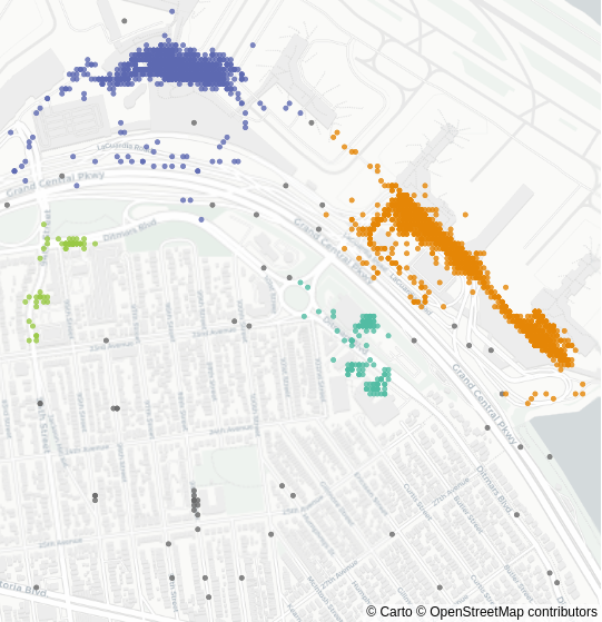
Figure 16: A clustering of the Rideshare data produced by Persistable, using the slice displayed in Fig. 12, choosing the large gap below the fourth vine. Gray points are unclustered.

$k$	Memory (GB)	Time (s)	Number of clusters
$20$	0.46	65	6524
$40$	0.82	58	2618
$80$	1.54	64	1057
$160$	2.99	68	473
$320$	5.88	79	230

Table 1: Performance evaluation of the HDBSCAN implementation of McInnes et al. (2017) on the Rideshare dataset. The columns are the algorithm parameter $k=\mathsf{min\_samples}$, the peak memory usage in GB, the runtime in seconds, and the number of clusters in the output. The algorithm parameter $\mathsf{min\_cluster\_size}$ is set equal to $\mathsf{min\_samples}$ (the default). The implementation includes several algorithms for computing HDBSCAN. Here we use the Dual-Tree Borůvka algorithm with kd-trees (the default choice for low-dimensional Euclidean data, as in this case). This is the only choice that gives reasonable performance on this dataset. Memory usage scales linearly with $k$ because the algorithm stores the $k$ nearest neighbors of each data point.

	1	2	3	noise
South Italy	293			30
Sardinia		97		1
North Italy			118	33

Table 2: A confusion matrix showing the relationship between the clustering we obtained with Persistable (clusters 1–3 and points labeled as noise), and the large area labels of the Olive oil data. The adjusted Rand index is $1.0$, and $89\%$ of the data is clustered.

		1	2	3	4	5	6	7	8	noise
South Italy	North Apulia	12								13
	Calabria		7	1						48
	South Apulia			100						106
	Sicily	3								33
Sardinia	Inland Sardinia				51					14
	Coast Sardinia					19				14
North Italy	East Liguria						14	1		35
	West Liguria							29		21
	Umbria								42	9

Table 3: A confusion matrix showing the relationship between the clustering we obtained with Persistable (clusters 1–8 and points labeled as noise), and the region labels of the Olive oil data. The adjusted Rand index is $0.98$, and $49\%$ of the data is clustered.

		1	2	3	4	5	6	7	8	noise
South Italy	North Apulia	21	2							2
	Calabria		50	3			1			2
	South Apulia		1	196						9
	Sicily	6	20	7						3
Sardinia	Inland Sardinia				65
	Coast Sardinia				2	31
North Italy	East Liguria						41	2		7
	West Liguria							47		3
	Umbria						2		48	1

Table 4: A confusion matrix showing the relationship between the clustering we obtained with Persistable, using the exhaustive persistence-based flattening (clusters 1–8 and points labeled as noise), and the region labels of the Olive oil data. The adjusted Rand index is $0.90$, and $95\%$ of the data is clustered.

References

- Anai et al. (2019) Hirokazu Anai, Frédéric Chazal, Marc Glisse, Yuichi Ike, Hiroya Inakoshi, Raphaël Tinarrage, and Yuhei Umeda. DTM-Based Filtrations. In Gill Barequet and Yusu Wang, editors, 35th International Symposium on Computational Geometry (SoCG 2019), volume 129 of Leibniz International Proceedings in Informatics (LIPIcs), pages 58:1–58:15, 2019. doi: 10.4230/LIPIcs.SoCG.2019.58.
- Balakrishnan et al. (2013) Sivaraman Balakrishnan, Srivatsan Narayanan, Alessandro Rinaldo, Aarti Singh, and Larry Wasserman. Cluster trees on manifolds. In C. J. C. Burges, L. Bottou, M. Welling, Z. Ghahramani, and K. Q. Weinberger, editors, Advances in Neural Information Processing Systems 26, pages 2679–2687. Curran Associates, Inc., 2013.
- Bauer et al. (2020) U. Bauer, M. Botnan, S. Oppermann, and J. Steen. Cotorsion torsion triples and the representation theory of filtered hierarchical clustering. Advances in Mathematics, 369:107171, 2020. doi: 10.1016/j.aim.2020.107171.
- Bauer and Lesnick (2015) Ulrich Bauer and Michael Lesnick. Induced matchings and the algebraic stability of persistence barcodes. Comput. Geom., 6:162–191, 2015. doi: 10.20382/jocg.v6i2a9.
- Biasotti et al. (2008) Silvia Biasotti, Andrea Cerri, Patrizio Frosini, Daniela Giorgi, and Claudia Landi. Multidimensional size functions for shape comparison. Journal of Mathematical Imaging and Vision, 32:161–179, 2008.
- Biau et al. (2007) Gérard Biau, Benoît Cadre, and Bruno Pelletier. A graph-based estimator of the number of clusters. ESAIM: Probability and Statistics, 11:272–280, 6 2007.
- Billingsley (1999) Patrick Billingsley. Convergence of Probability Measures, Second Edition. Wiley Series in Probability and Statistics. Wiley, 1999.