The Trimmed Lasso: Sparse Recovery Guarantees and Practical Optimization by the Generalized Soft-Min Penalty

Abstract

We present a new approach to solve the sparse approximation or best subset selection problem, namely find a $k$-sparse vector ${\bf x}\in\mathbb{R}^{d}$ that minimizes the $\ell_{2}$ residual $\lVert A{\bf x}-{\bf y}\rVert_{2}$. We consider a regularized approach, whereby this residual is penalized by the non-convex trimmed lasso, defined as the $\ell_{1}$-norm of ${\bf x}$ excluding its $k$ largest-magnitude entries. We prove that the trimmed lasso has several appealing theoretical properties, and in particular derive sparse recovery guarantees assuming successful optimization of the penalized objective. Next, we show empirically that directly optimizing this objective can be quite challenging. Instead, we propose a surrogate for the trimmed lasso, called the generalized soft-min. This penalty smoothly interpolates between the classical lasso and the trimmed lasso, while taking into account all possible $k$-sparse patterns. The generalized soft-min penalty involves summation over $\binom{d}{k}$ terms, yet we derive a polynomial-time algorithm to compute it. This, in turn, yields a practical method for the original sparse approximation problem. Via simulations, we demonstrate its competitive performance compared to current state of the art.

1 Introduction

Consider the sparse approximation or best subset selection problem: Given an $n\times d$ matrix $A$, a vector $\mbox{\boldmath$y$}\in\mathbb{R}^{n}$ and a sparsity parameter $k\ll\min{\left\{{n,d}\right\}}$, solve

$$\underset{\mbox{\boldmath$x$}}{\min}\ {\left\|{A\mbox{\boldmath$x$}-\mbox{\boldmath$y$}}\right\|}_{2}\quad\mbox{s.t.}\quad{\left\|{\mbox{\boldmath$x$}}\right\|}_{0}\leq k.$$ (P0)

The inverse problem Equation P0 and related variants play a key role in multiple fields. Examples include signal and image processing [bruckstein2009sparse, elad2010sparsebook, Mallat_book], compressed sensing [eldar2012compressed, Foucart_Rauhut], medical imaging [lustig2007sparse, provost2009application], computer vision [Wright], high dimensional statistics [Hastie_book], biology [Wu_Lasso] and economics [brodie2009sparse, fan2011sparse]. While in few cases the sparsity level $k$ is known, it often needs to be estimated. Typically one solves Equation P0 for several values of $k$ and applies cross validation [ward2009compressed] or a model selection criterion. Here we focus on solving Equation P0 for a given value of $k$.

Even though solving Equation P0 is NP-hard [davis1997adaptive, natarajan1995sparse], several approaches were developed to seek approximate solutions. One approach is to search for the best $k$ variables greedily, adding one or several variables at a time, and possibly discarding some of the previously chosen ones. Examples include iterative thresholding, matching pursuit and forward-backward methods; see [blumensath2008ihtfirst, dai2009subspace, davis1994, mallat1993matching, Miller_book, needell2009cosamp, needell2010signal, pati1993orthogonal, rebollo2002optimized, Tropp_Gilbert] and references therein.

A different approach is to replace the constraint ${\left\|{\mbox{\boldmath$x$}}\right\|}_{0}\leq k$ by a penalty term $\rho(\mbox{\boldmath$x$})$, and instead of Equation P0 solve the regularized problem

$$\min_{\mbox{\boldmath$x$}}\ \tfrac{1}{2}{\left\|{A\mbox{\boldmath$x$}-\mbox{\boldmath$y$}}\right\|}^{2}+\lambda\rho(\mbox{\boldmath$x$}).$$ (1.1)

With few exceptions detailed below, most penalties are separable and do not depend on $k$. For some scalar function $f(x)$, they take the form $\rho(\mbox{\boldmath$x$})=\sum_{i=1}^{d}f{\left({x_{i}}\right)}$. A $k$-sparse solution can be obtained by tuning the penalty parameter $\lambda$ and projecting the obtained solutions to be $k$-sparse. The most popular penalty is the $\ell_{1}$ norm [chen2001atomic, tibshirani1996regression]. Many fast algorithms were developed to optimize Equation 1.1 with a convex $\rho(\mbox{\boldmath$x$})$; see [beck2009fast, Friedman_Reg_Path, Yin_Osher] and references therein.

In many practical settings, matching pursuit algorithms and the $\ell_{1}$-penalty approaches may output solutions that are quite suboptimal for the original problem Equation P0. Thus, various nonconvex penalties have been proposed, such as $\ell_{p}$ penalties with $p<1$ [chartrand2007exact, figueiredo2005bound], minimax concave penalty [zhang2010nearly], smoothly clipped absolute deviation [fan2001variable, hunter2005variable, zou2008one] and the smoothed $\ell_{0}$ penalty [mohimani2009fast]. For even better solutions to Equation P0, non-separable penalties were proposed [bogdan2015slope, selesnick2017sparse, wipf2010iterative, Zeng]. Local minima of these penalized objectives are often found by iteratively reweighted least squares (IRLS) [chartrand2007exact, chartrand2008iteratively, daubechies2010iteratively, figueiredo2007majorization] or iteratively reweighted $\ell_{1}$ (IRL1) [candes2008enhancing, figueiredo2007majorization, foucart2009sparsest].

A different approach to Equation P0 is to pose it as a mixed integer program (MIP) and solve it globally; see for example [furnival1974regressions, arthanari1981mathematical, bienstock1996computational]. MIP-based methods update both the current solution and a lower bound on the optimal objective. When the current objective equals this lower bound, the algorithm terminates with a certificate of global optimality. With vast improvements in algorithmic efficiency and computing power, this approach gained increased popularity, and various works illustrated its applicability to problems with thousands of variables [liu2007variable, bertsimas2009algorithm, bertsimas2016best, mazumder2017discrete, bertsimas2020sparse]. Recently, [bertsimas2020sparse] developed a cutting-plane method able to globally solve problems with $d=100000$ variables in less than a minute, provided the sparsity $k$ is not too high. MIP may also be combined with other approaches. One recent example is [hazimeh2020fast], whereby first a local optimum is found by coordinate descent, and then improved upon by a local combinatorial search, which replaces only a subset of the selected variables. This method is extremely fast and can handle problems with even a million variables or more. However, it is not guaranteed to find the globally optimal solution. Rather, it finds a local minimum that cannot be improved by replacing a small number of variables. Yet, as we demonstrate in Section 5, despite these significant advancements in MIP-based approaches, our proposed method can successfully handle challenging settings in practical time, where the above methods either take a prohibitive runtime, or find highly suboptimal solutions.

In this work we focus on the non-separable trimmed lasso penalty ${{\tau}_{k}}(\mbox{\boldmath$x$})$, whereby a candidate vector $x$ is penalized by its $\ell_{1}$-distance to the nearest $k$-sparse vector. Namely,

$${{\tau}_{k}}(\mbox{\boldmath$x$})=\sum_{i=k+1}^{d}{{\left|{\mbox{\boldmath$x$}}\right|}_{\left({i}\right)}},$$ (1.2)

where ${{\left|{\mbox{\boldmath$x$}}\right|}_{\left({1}\right)}}\geq{{\left|{\mbox{\boldmath$x$}}\right|}_{\left({2}\right)}}\geq\ldots\geq{{\left|{\mbox{\boldmath$x$}}\right|}_{\left({d}\right)}}$ are the absolute values of the entries of $x$, sorted in decreasing order. The original problem Equation P0 is replaced by either the regularized problem

$$\min_{\mbox{\boldmath$x$}}\ {\mathrm{F}_{\lambda}}(\mbox{\boldmath$x$}){\ =\ }\tfrac{1}{2}{\left\|{A\mbox{\boldmath$x$}-\mbox{\boldmath$y$}}\right\|}_{2}^{2}+\lambda{{\tau}_{k}}(\mbox{\boldmath$x$}),$$ (1.3)

or by the following variant, which involves the residual norm to the power 1 rather than 2,

$$\underset{\mbox{\boldmath$x$}}{\min}\ {\mathrm{F}^{1}_{\lambda}}(\mbox{\boldmath$x$}){\ =\ }{\left\|{A\mbox{\boldmath$x$}-\mbox{\boldmath$y$}}\right\|}_{2}+\lambda{{\tau}_{k}}(\mbox{\boldmath$x$}).$$ (1.4)

An important property of the trimmed lasso is that it explicitly promotes the sparsity level $k$ of the original problem Equation P0, with ${{\tau}_{k}}(\mbox{\boldmath$x$})=0$ if and only if $x$ is $k$-sparse. The penalty ${{\tau}_{k}}(\mbox{\boldmath$x$})$ was discussed in [gotoh2018dc, tono2017efficient], who developed a difference-of-convex (DC) programming scheme to optimize Equation 1.3. A closely related penalty that combines the lasso and the trimmed lasso was studied independently in [huang2015two], where a similar DC programming scheme was proposed. The name trimmed lasso was coined by [bertsimas2017trimmed], who proposed an alternating direction method of multipliers (ADMM) scheme. Recently, [yun2019trimming] studied the statistical properties of the trimmed lasso and developed a block coordinate descent algorithm to optimize Equation 1.3.

In this work we make several theoretical and algorithmic contributions towards solving the best subset selection problem Equation P0. First, in Section 2 we advocate solving Equation P0 by minimizing trimmed-lasso penalized objectives. In particular, we prove that for a sufficiently large penalty parameter $\lambda$, the local minimizers of Equation 1.3 and of Equation 1.4 are $k$-sparse. Hence, the global minima coincide with those of the original problem Equation P0. Our results extend those of [gotoh2018dc, bertsimas2017trimmed]. Second, we present novel recovery guarantees when optimizing Equation 1.3 or Equation 1.4 for any positive $\lambda$. Specifically, assuming that $\mbox{\boldmath$y$}=A\mbox{\boldmath$x$}_{0}+\mbox{\boldmath$e$}$, with $\mbox{\boldmath$x$}_{0}$ approximately $k$-sparse, we study how well $\mbox{\boldmath$x$}_{0}$ can be estimated by optimizing Equation 1.3 or Equation 1.4. We prove that even at low values of $\lambda$, where optimal solutions of these problems may not coincide with those of Equation P0, $\mbox{\boldmath$x$}_{0}$ can still be well-approximated by these solutions, with the recovery stable to the measurement error $e$.

Our theoretical results motivate the development of practical methods to optimize the trimmed-lasso regularized objectives Equation 1.3 and Equation 1.4. Unfortunately, directly optimizing these objectives can be challenging. One of our key contributions is the development of a new method to solve Equation 1.3 and Equation 1.4. As we show in Section 5, our method is able to find solutions with significantly lower objective values than of those computed by DC programming and ADMM.

In our approach we replace the trimmed lasso $\tau_{k}(\mbox{\boldmath$x$})$ by a surrogate penalty called the generalized soft-min and denoted $\tau_{k,\gamma}(\mbox{\boldmath$x$})$. Our proposed penalty depends not only on the sparsity level $k$ but also on a smoothness parameter $\gamma$. As described in Section 3, ${{\tau}_{k,\gamma}}(\mbox{\boldmath$x$})$ has two important properties: First, for any finite $\gamma$, it is $C^{\infty}$-smooth as a function of ${\left|{\mbox{\boldmath$x$}}\right|}={\left({|x_{1}|,\ldots,|x_{d}|}\right)}$. This facilitates the use of continuous optimization techniques. Second, as $\gamma$ increases, ${{\tau}_{k,\gamma}}(\mbox{\boldmath$x$})$ varies smoothly from the convex $\ell_{1}$-norm (at $\gamma=0$) to the trimmed lasso (at $\gamma=\infty$). For any $\gamma>0$, ${{\tau}_{k,\gamma}}(\mbox{\boldmath$x$})$ takes into account all $\binom{d}{k}$ sparsity patterns of $x$. Its naïve computation is thus intractable. Another important contribution, described in Section 4, is the development of a polynomial time algorithm to calculate it in $\mathcal{O}(kd)$ operations.

Given the aforementioned properties of ${{\tau}_{k,\gamma}}$, in Section 3 we describe the following approach to solve the trimmed lasso penalized Equation 1.3: We replace ${{\tau}_{k}}$ by ${{\tau}_{k,\gamma}}$, start from an easy convex problem at $\gamma=0$, and smoothly transform it to Equation 1.3 by increasing $\gamma$ towards infinity. At $\gamma=0$, our penalty coincides with the lasso, leading to a convex problem. Next, we gradually increase $\gamma$ while tracing the path of solutions. At each intermediate $\gamma$, we optimize the corresponding objective by a majorization-minimization scheme, initialized at the solution found for the previous $\gamma$. Empirically, the resulting path of solutions often converges to a better solution of Equation 1.3 than that obtained by directly optimizing Equation 1.3 with the nonsmooth trimmed lasso.

Finally, we seek solutions to the original problem Equation P0 by solving Equation 1.3 for several values of $\lambda$, followed by projecting each solution to the nearest $k$-sparse vector and solving a least-squares problem on its support. The $k$-sparse vector with the smallest residual norm ${\left\|{A\mbox{\boldmath$x$}-\mbox{\boldmath$y$}}\right\|}_{2}$ is chosen. As we demonstrate empirically in Section 5, optimizing our smooth surrogate of the trimmed lasso yields state-of-the-art results in sparse recovery.

Notations and Definitions

We denote by ${\bf a}_{i}$ the $i$-th column of the $n\times d$ matrix $A$. We denote $[d]=\{1,\ldots,d\}$. For a scalar $x$, ${{\left[{{x}}\right]}_{+}}=\max{\left\{{x,0}\right\}}$ and ${{\left[{{x}}\right]}_{-}}=\max{\left\{{-x,0}\right\}}$. For a vector $x$, ${\Pi_{k}}(\mbox{\boldmath$x$})$ is its $k$-sparse projection, namely the $k$-sparse vector closest to $x$ in $\ell_{1}$-norm, breaking ties arbitrarily. For a function $f:{\mathbb{R}^{d}}\rightarrow{\mathbb{R}}$, we denote its directional derivative at a point $\mbox{\boldmath$x$}\in{\mathbb{R}^{d}}$ in direction $\mbox{\boldmath$v$}\in{\mathbb{R}^{d}}$ by

$$\begin{split}\nabla_{\mbox{\boldmath$v$}}f(\mbox{\boldmath$x$}){\ =\ }\lim_{t\searrow 0}\frac{f{\left({\mbox{\boldmath$x$}+t\mbox{\boldmath$v$}}\right)}-f{\left({\mbox{\boldmath$x$}}\right)}}{t}.\end{split}$$

2 Theory for the trimmed lasso

In this section we study the following two key theoretical questions related to the trimmed lasso penalty: (i) what is the relation between minimizers of Equation 1.3 or Equation 1.4 and those of the original problem Equation P0, and do the two coincide for sufficiently large $\lambda$? and (ii) assuming that $\mbox{\boldmath$x$}_{0}$ is approximately $k$-sparse, can it be recovered from an observed vector $\mbox{\boldmath$y$}=A\mbox{\boldmath$x$}_{0}+\mbox{\boldmath$e$}$ by optimizing problems Equation 1.3 or Equation 1.4? The practical question of how to optimize Equation 1.3 or Equation 1.4 is addressed in Section 3. Proofs are in Section B.1.

2.1 Penalty thresholds

Denote by ${\bar{\lambda}}$ the threshold

$${\bar{\lambda}}{\ =\ }{\left\|{\mbox{\boldmath$y$}}\right\|}_{2}\cdot\max_{i=1,\ldots,d}{\left\|{\mbox{\boldmath$a$}_{i}}\right\|}_{2}.$$ (2.1)

The following Theorem shows that for large $\lambda$, problem Equation 1.3 is intimately related to Equation P0.

Theorem 2.1.

If $\lambda>{\bar{\lambda}}$, then any local minimum of Equation 1.3 is $k$-sparse.

A key implication of this theorem is that for $\lambda>{\bar{\lambda}}$, the optimal solutions of Equation P0 and Equation 1.3 coincide. With some differences, similar results were proven in [bertsimas2017trimmed, gotoh2018dc]. In [gotoh2018dc] the guarantee required the set of optimal solutions of Equation P0 to be bounded, and the threshold depends on this bound. Hence, in some cases, it may be larger than ${\bar{\lambda}}$. The authors of [bertsimas2017trimmed] proved a result similar to Theorem 2.1, with the same threshold ${\bar{\lambda}}$, but for a trimmed-lasso regularized objective with an additional $\ell_{1}$-penalty term.

To derive an analogous result for problem Equation 1.4, we introduce the following two thresholds

$${}\begin{split}{\lambda_{a}}{\ =\ }\frac{\sigma_{n}{\left({A}\right)}}{\sqrt{d-k}},\qquad{\lambda_{b}}{\ =\ }\max_{i=1,\ldots,d}{\left\|{\mbox{\boldmath$a$}_{i}}\right\|}_{2},\end{split}$$ (2.2)

where $\sigma_{n}{\left({A}\right)}$ is the $n$-th singular value of $A$.

Theorem 2.2.

Suppose that $\lambda>{\lambda_{b}}$. Then any local minimum of Equation 1.4 is $k$-sparse.

Theorem 2.3.

Suppose that the $n\times d$ matrix $A$, with $d\geq n$ is of full rank, so that ${\lambda_{a}}>0$. Assume that $0<\lambda<{\lambda_{a}}$. Then any local minimum ${\mbox{\boldmath$x$}^{*}}$ of Equation 1.4 satisfies $A{\mbox{\boldmath$x$}^{*}}=\mbox{\boldmath$y$}$.

Theorem 2.2 implies that for $\lambda>{\lambda_{b}}$, the optimal solutions of the trimmed lasso objective Equation 1.4 coincide with those of Equation P0. In contrast, by Theorem 2.3, for $\lambda<{\lambda_{a}}$ the trimmed lasso penalty has little effect, as the minimizers of the objective lie in the subspace of zero residual.

Theorem 2.1 seems to suggest that to solve Equation P0, one should optimize the trimmed lasso objective ${\mathrm{F}_{\lambda}}$ with $\lambda>{\bar{\lambda}}$. However, since ${{\tau}_{k}}$ is nonconvex, larger values of $\lambda$ increase the dominance of the nonconvex part of the objective, making it more difficult to optimize. The following theorem sheds further light on this difficulty, showing that for $\lambda\geq{\bar{\lambda}}$, the optimization landscape is riddled with poor local minima.

Theorem 2.4.

Let $\Lambda\subset{\left[{d}\right]}$ be any index set of size $k$, and let $\tilde{\mbox{\boldmath$x$}}$ be the minimizer of ${\left\|{A\mbox{\boldmath$x$}-\mbox{\boldmath$y$}}\right\|}_{2}$ over all vectors $x$ with $\mbox{supp}(\mbox{\boldmath$x$})\subseteq\Lambda$. If $\|\mbox{\boldmath$\tilde{\mbox{\boldmath$x$}}$}\|_{0}=k$, then it is a local minimum of ${\mathrm{F}_{\lambda}}$ for any $\lambda\geq{\bar{\lambda}}$. The same claim holds for ${\mathrm{F}^{1}_{\lambda}}$ with $\lambda\geq{\lambda_{b}}$.

Finally, regarding the power-1 case, our algorithm to minimize ${\mathrm{F}^{1}_{\lambda,\gamma}}$, presented in Section 3, is guaranteed under mild assumptions to output the same solution for all $\lambda<{\lambda_{a}}$; see Appendix C.

In light of the above discussion and theorems, our strategy to solve Equation P0 is to minimize ${\mathrm{F}_{\lambda}}$ or ${\mathrm{F}^{1}_{\lambda}}$ for several values of $\lambda<{\bar{\lambda}}$ or $\lambda\in{\left[{{\lambda_{a}},{\lambda_{b}}}\right]}$, respectively. As we discuss theoretically in the next subsection, an appealing property of the trimmed lasso is that even at low values of $\lambda$, where the solutions are not necessarily $k$-sparse, they may still be close to the optimal solution of Equation P0.

2.2 Sparse recovery guarantees

A fundamental and well-studied problem is the ability of various methods to recover a sparse vector $\mbox{\boldmath$x$}_{0}$ from few linear and potentially noisy measurements; see [Foucart_Rauhut, elad2010sparsebook, eldar2012compressed] and references therein. Here we present sparse recovery guarantees for the trimmed lasso relaxations Equation 1.3 and Equation 1.4. Specifically, let $\mbox{\boldmath$x$}_{0}\in{\mathbb{R}^{d}}$ be approximately $k$-sparse, in the sense that ${{\tau}_{k}}(\mbox{\boldmath$x$}_{0})\ll{\left\|{\mbox{\boldmath$x$}_{0}}\right\|}_{1}$. Given $A$ and $k$, our goal is to estimate $\mbox{\boldmath$x$}_{0}$ from

$${}\begin{split}\mbox{\boldmath$y$}=A\mbox{\boldmath$x$}_{0}+\mbox{\boldmath$e$},\end{split}$$ (2.3)

where $e$ is an unknown measurement error. In our analysis, we consider an adversarial model, whereby do not make any probabilistic assumptions on $e$. Our bounds thus depend on $\|\mbox{\boldmath$e$}\|_{2}$.

Without further assumptions on $A$, this problem is ill posed. As is well known, even in the absence of noise, a necessary condition for unique recovery of a $k$-sparse $\mbox{\boldmath$x$}_{0}$ is that any subset of $2k$ columns of $A$ are linearly independent [Foucart_Rauhut, Theorem 2.13]. Similarly to previous works, we require that any $2k$ columns of $A$ are sufficiently far from being linearly dependent. Specifically, we assume that there exists a constant ${\alpha_{2k}}>0$ such that for any $x$ with ${\left\|{\mbox{\boldmath$x$}}\right\|}_{0}\leq 2k$,

$${\left\|{A\mbox{\boldmath$x$}}\right\|}_{2}\geq{\alpha_{2k}}{\left\|{\mbox{\boldmath$x$}}\right\|}_{1}.$$ (2.4)

Equation Equation 2.4 is a one-sided variant of the restricted isometry property (RIP), commonly used to derive sparse recovery guarantees. RIP was introduced in [candes2005decoding] and further studied in [blanchard2011compressed, candes2008restricted, candes2006quantitative, candes2006robust, candes2006stable, foucart2009sparsest, cohen2009compressed]. Variants with norms other than $\ell_{2}$ [allen2016restricted, berinde2008combining, chartrand2008restricted, dirksen2016gap] were used to provide sharper guarantees. As shown below, Equation 2.4 is the natural combination of powers for studying the trimmed lasso in conjunction with an $\ell_{2}$-residual ${\left\|{A\mbox{\boldmath$x$}-\mbox{\boldmath$y$}}\right\|}_{2}$. We remark that calculating ${\alpha_{2k}}$, or even approximating it, is NP-hard [tillmann2014computational]. However, ${\alpha_{2k}}$ can be bounded from below by the cumulative coherence, also known as the Babel function [tropp2004greed].

We now present our main theoretical result, which links success in optimizing problems Equation 1.3 or Equation 1.4 at a given $\lambda>0$, with accurate estimation of $\mbox{\boldmath$x$}_{0}$. By success we mean that the solution $\hat{\mbox{\boldmath$x$}}$, computed by some algorithm, satisfies that ${\mathrm{F}_{\lambda}}{\left({\mbox{\boldmath$\hat{\mbox{\boldmath$x$}}$}}\right)}\leq{\mathrm{F}_{\lambda}}{\left({{\Pi_{k}}{\left({\mbox{\boldmath$x$}_{0}}\right)}}\right)}$. The following theorem shows that under this condition, ${\Pi_{k}}(\hat{}\mbox{\boldmath$x$})$ is close to $\mbox{\boldmath$x$}_{0}$.

Theorem 2.5.

Let $\mbox{\boldmath$y$}=A\mbox{\boldmath$x$}_{0}+\mbox{\boldmath$e$}$ and let ${\alpha_{2k}}$, ${\lambda_{b}}$ be the constants defined in Equations 2.4 and 2.2. Let $\lambda>0$ and suppose that $\mbox{\boldmath$\hat{\mbox{\boldmath$x$}}$}\in{\mathbb{R}^{d}}$ satisfies ${\mathrm{F}_{\lambda}}{\left({\mbox{\boldmath$\hat{\mbox{\boldmath$x$}}$}}\right)}\leq{\mathrm{F}_{\lambda}}{\left({{\Pi_{k}}{\left({\mbox{\boldmath$x$}_{0}}\right)}}\right)}$. Then,

1. The projected vector ${\Pi_{k}}{\left({\mbox{\boldmath$\hat{\mbox{\boldmath$x$}}$}}\right)}$ is close to $\mbox{\boldmath$x$}_{0}$ in $\ell_{1}$ norm,

   $${}\begin{split}{\left\|{{\Pi_{k}}{\left({\mbox{\boldmath$\hat{\mbox{\boldmath$x$}}$}}\right)}-\mbox{\boldmath$x$}_{0}}\right\|}_{1}\leq{{\tau}_{k}}{\left({\mbox{\boldmath$x$}_{0}}\right)}+\tfrac{2}{{\alpha_{2k}}}{\left({{\left\|{\mbox{\boldmath$e$}}\right\|}_{2}+{\lambda_{b}}{{\tau}_{k}}{\left({\mbox{\boldmath$x$}_{0}}\right)}}\right)}+\tfrac{1}{2\lambda{\alpha_{2k}}}{\left({{\left\|{\mbox{\boldmath$e$}}\right\|}_{2}+{\lambda_{b}}{{\tau}_{k}}{\left({\mbox{\boldmath$x$}_{0}}\right)}}\right)}^{2}.\end{split}$$ (2.5)

2. If $\hat{\mbox{\boldmath$x$}}$ itself is $k$-sparse, then the following tighter bound holds,

   $${}\begin{split}{\left\|{\mbox{\boldmath$\hat{\mbox{\boldmath$x$}}$}-\mbox{\boldmath$x$}_{0}}\right\|}_{1}\leq\tfrac{2}{{\alpha_{2k}}}{\left\|{\mbox{\boldmath$e$}}\right\|}_{2}+(1+2\tfrac{{\lambda_{b}}}{{\alpha_{2k}}}){{\tau}_{k}}{\left({\mbox{\boldmath$x$}_{0}}\right)}.\end{split}$$ (2.6)

The next theorem provides an analogous recovery guarantee for the power-1 objective Equation 1.4.

Theorem 2.6.

Let $\mbox{\boldmath$y$}=A\mbox{\boldmath$x$}_{0}+\mbox{\boldmath$e$}$, and let ${\alpha_{2k}}$, ${\lambda_{b}}$ be the constants defined in Equations 2.4 and 2.2. Suppose that $\mbox{\boldmath$\hat{\mbox{\boldmath$x$}}$}\in{\mathbb{R}^{d}}$ satisfies ${\mathrm{F}^{1}_{\lambda}}{\left({\mbox{\boldmath$\hat{\mbox{\boldmath$x$}}$}}\right)}\leq{\mathrm{F}^{1}_{\lambda}}{\left({{\Pi_{k}}{\left({\mbox{\boldmath$x$}_{0}}\right)}}\right)}$ for some $\lambda>0$. Then,

1. The projected vector ${\Pi_{k}}{\left({\mbox{\boldmath$\hat{\mbox{\boldmath$x$}}$}}\right)}$ is close to $\mbox{\boldmath$x$}_{0}$ in $\ell_{1}$ norm,

   $${\left\|{{\Pi_{k}}{\left({\mbox{\boldmath$\hat{\mbox{\boldmath$x$}}$}}\right)}-\mbox{\boldmath$x$}_{0}}\right\|}_{1}\leq{{\tau}_{k}}{\left({\mbox{\boldmath$x$}_{0}}\right)}+\tfrac{1}{{\alpha_{2k}}}{\left({1+\max{\left\{{1,\tfrac{{\lambda_{b}}}{\lambda}}\right\}}}\right)}{\bigl{(}{{\left\|{\mbox{\boldmath$e$}}\right\|}_{2}+{\lambda_{b}}{{\tau}_{k}}{\left({\mbox{\boldmath$x$}_{0}}\right)}}\bigr{)}}.$$ (2.7)

2. If $\hat{\mbox{\boldmath$x$}}$ itself is $k$-sparse, then the tighter bound Equation 2.6 holds.

Theorems 2.5 and 2.6 do not assume that an algorithm found the global minimum of the respective objectives, only that it was able to find an approximate solution, with an objective value close to the optimal one. Thus, Theorems 2.5 and 2.6 imply that successful optimization of Equation 1.3 or Equation 1.4 yields a successful recovery of $\mbox{\boldmath$x$}_{0}$, which is stable with respect to the measurement error $e$ and the deviation of $\mbox{\boldmath$x$}_{0}$ from being exactly $k$-sparse.

Another implication of Theorems 2.5 and 2.6 is that $\mbox{\boldmath$x$}_{0}$ can be accurately estimated by solving Equation 1.3 or Equation 1.4 even at low values of $\lambda$, where the global minimizers are not necessarily $k$-sparse. While the above guarantees improve as $\lambda$ increases, as discussed in the previous subsection, optimizing these problems at low values of $\lambda$ is potentially an easier task. Indeed, in our simulations described in Section 5, the best solutions, with smallest ${\left\|{A{\Pi_{k}}(\hat{}\mbox{\boldmath$x$})-\mbox{\boldmath$y$}}\right\|}_{2}$, were often obtained at low values of $\lambda$, where $\hat{\mbox{\boldmath$x$}}$ itself was not $k$-sparse.

Recently, [yun2019trimming] also analyzed the trimmed lasso penalized objective and derived support recovery guarantees. There are some key differences between our analysis and theirs. They assumed that the rows of $A$ are i.i.d. samples from a $d$-dimensional sub-Gaussian distribution, that the true $\mbox{\boldmath$x$}_{0}$ is exactly $k$-sparse, and that the noise $e$ has i.i.d. entries.

We now compare the guarantee of Theorems 2.5 and 2.6 to those for basis pursuit. Suppose that $A$ has $\ell_{2}$-normalized columns and satisfies the RIP of order $2k$ with constant $\delta_{2k}<1$,

$${\left({1-\delta_{2k}}\right)}{\left\|{\mbox{\boldmath$x$}}\right\|}^{2}_{2}\leq{\left\|{A\mbox{\boldmath$x$}}\right\|}_{2}^{2}\leq{\left({1+\delta_{2k}}\right)}{\left\|{\mbox{\boldmath$x$}}\right\|}^{2}_{2}\qquad\forall\mbox{\boldmath$x$}\text{ s.t. }{\left\|{\mbox{\boldmath$x$}}\right\|}_{0}\leq 2k.$$ (2.8)

Let $\mbox{\boldmath$\hat{\mbox{\boldmath$x$}}$}_{\textup{BP}}$ be the solution of the following quadratically constrained Basis Pursuit problem,

$$\mbox{\boldmath$\hat{\mbox{\boldmath$x$}}$}_{\textup{BP}}=\operatorname*{\arg\!\min}_{\mbox{\boldmath$x$}}\ {\left\|{\mbox{\boldmath$x$}}\right\|}_{1}\quad\text{s.t.}\quad{\left\|{A\mbox{\boldmath$x$}-\mbox{\boldmath$y$}}\right\|}_{2}\leq{\left\|{\mbox{\boldmath$e$}}\right\|}_{2}$$

By [Foucart_Rauhut, Theorem 6.12], if $\delta_{2k}<4/\sqrt{41}\approx 0.6246$, then the following guarantee holds, with $c_{1},c_{2}$ constants that depend only on $\delta_{2k}$,

$${\left\|{\mbox{\boldmath$\hat{\mbox{\boldmath$x$}}$}_{\textup{BP}}-\mbox{\boldmath$x$}_{0}}\right\|}_{1}\leq c_{1}\sqrt{k}{\left\|{\mbox{\boldmath$e$}}\right\|}_{2}+c_{2}{{\tau}_{k}}{\left({\mbox{\boldmath$x$}_{0}}\right)}.$$ (2.9)

A lower bound on $\delta_{2k}$ is necessary for such a recovery guarantee to hold. Indeed, as shown in [davies2009restricted], there exist matrices with $\delta_{2k}$ arbitrarily close to $1/\sqrt{2}\approx 0.7071$, for which BP fails. Recovery guarantees of other polynomial-time methods such as OMP and iterative thresholding require similar, and often stricter, conditions on the RIP constant; see [Foucart_Rauhut, Chapter 6].

Let us compare Equation 2.9 to our guarantees. It is easy to show that Equation 2.8 implies that $\alpha_{2k}$, defined in Equation 2.4, satisfies $\alpha_{2k}\geq{\sqrt{1-\delta_{2k}}}/{\sqrt{2k}}$. Consider a vector $\hat{\mbox{\boldmath$x$}}$ that is a global minimizer of either Equation 1.3 or Equation 1.4. To simplify the analysis, suppose that $\lambda$ is high enough so that $\hat{\mbox{\boldmath$x$}}$ is $k$-sparse. Then both Theorems 2.5 and 2.6 yield

$${\left\|{\mbox{\boldmath$\hat{\mbox{\boldmath$x$}}$}-\mbox{\boldmath$x$}_{0}}\right\|}_{1}\leq 2\tfrac{\sqrt{2k}}{\sqrt{1-\delta_{2k}}}{\left\|{\mbox{\boldmath$e$}}\right\|}_{2}+{\left({1+2\sqrt{2k}\sqrt{\tfrac{1+\delta_{2k}}{1-\delta_{2k}}}}\right)}{{\tau}_{k}}{\left({\mbox{\boldmath$x$}_{0}}\right)}.$$ (2.10)

While in our bound the coefficient of ${{\tau}_{k}}{\left({\mbox{\boldmath$x$}_{0}}\right)}$ is larger by a multiplicative factor of $\mathcal{O}{\left({\sqrt{k}}\right)}$, the key point is that our guarantee holds for any $\delta_{2k}<1$. We remark that the condition $\delta_{2k}<1$ is necessary for successful recovery of $\mbox{\boldmath$x$}_{0}$ by any algorithm (see e.g. [cohen2009compressed, Lemma 3.1]).

2.3 Solving the best subset selection problem by the trimmed lasso penalty

The above theoretical results motivate solving Equation P0 by optimizing the trimmed-lasso penalized ${\mathrm{F}_{\lambda}}$ or ${\mathrm{F}^{1}_{\lambda}}$. For ${\mathrm{F}_{\lambda}}$ we propose the following approach: Choose $0<\lambda_{1}<\lambda_{2}<\ldots\leq\lambda_{T}={\bar{\lambda}}$. For each $\lambda_{i}$, optimize ${\mathrm{F}_{\lambda}}$ with $\lambda=\lambda_{i}$. Next, project each solution $\mbox{\boldmath$\hat{\mbox{\boldmath$x$}}$}_{\lambda_{i}}$ to its nearest $k$-sparse vector, and solve a least-squares problem on its support. Output the vector with smallest residual $\|A\mbox{\boldmath$x$}-\mbox{\boldmath$y$}\|_{2}$. For the power-1 objective ${\mathrm{F}^{1}_{\lambda}}$, we propose a similar approach with $\lambda\in[{\lambda_{a}},{\lambda_{b}}]$.

To carry out this approach, one needs a practical algorithm to optimize trimmed lasso penalized objectives. In the next section we present a new approach to do so. As we demonstrate in Section 5, our method often finds much better solutions than those found by previously proposed methods such as DC programming [gotoh2018dc] and ADMM [bertsimas2017trimmed]. This, in turn, yields state-of-the-art results in solving the best subset selection problem Equation P0.

3 The generalized soft-min penalty

Optimizing trimmed-lasso penalized objectives is difficult for several reasons. First, ${{\tau}_{k}}(\mbox{\boldmath$x$})$ is nonconvex. Second, updating a solution $x$ along the negative gradient $-\nabla{{\tau}_{k}}(\mbox{\boldmath$x$})$ does not change its top-$k$ largest magnitude coordinates, since $\nabla{{\tau}_{k}}(\mbox{\boldmath$x$})$ is zero there, and shrinks the remaining $d-k$ coordinates. While this property is desirable if the current solution has the correct support, it may be detrimental otherwise.

To overcome this difficulty, we propose a soft surrogate for the trimmed lasso. To motivate it, consider the following equivalent definition of ${{\tau}_{k}}$ [bertsimas2017trimmed],

$${{\tau}_{k}}(\mbox{\boldmath$x$})=\underset{{\left|{\Lambda}\right|}=d-k}{\min}\ \sum_{i\in\Lambda}\ {\left|{x_{i}}\right|},$$ (3.1)

where $\Lambda\subset[d]$ is a set of $d-k$ distinct indices. Equation Equation 3.1 shows that ${{\tau}_{k}}(\mbox{\boldmath$x$})$ can be expressed as a hard assignment: Out of all $\binom{d}{k}$ subsets of size $d-k$, it takes the one with the smallest $\ell_{1}$ residual. In $k$-means data clustering, [zhang1999k] relaxed a hard assignment of each point to its nearest cluster center, to a soft assignment, with weights depending on the distances to all cluster centers. This led to significantly improved clustering results [hamerly2002alternatives]. Similarly, in multi-class classification, the one-hot vector is often replaced by the soft-max function [bridle1989probabilistic].

Inspired by these works, we propose the following surrogate, which we call the generalized soft-min (GSM) penalty ${{\tau}_{k,\gamma}}(\mbox{\boldmath$x$})$. In addition to $k$, it depends on a softness parameter $\gamma\in{\left[{0,\infty}\right]}$. For $\gamma\in{\left({0,\infty}\right)}$, it is defined by

$${}\begin{split}{{\tau}_{k,\gamma}}(\mbox{\boldmath$x$}){\ =\ }-\frac{1}{\gamma}\log{\left({\frac{1}{\binom{d}{d-k}}\sum_{{{\left|{\Lambda}\right|}=d-k}}\exp{\left({-\gamma\sum_{i\in\Lambda}{\left|{x_{i}}\right|}}\right)}}\right)}.\end{split}$$ (3.2)

The sum in Equation 3.2 is over all $\binom{d}{k}$ sets $\Lambda\subseteq{\left[{d}\right]}$ of $d-k$ distinct indices. We define ${{\tau}_{k,0}}(\mbox{\boldmath$x$})$ and ${{\tau}_{k,\infty}}(\mbox{\boldmath$x$})$ by the respective limits, described in the following Lemma.

Lemma 3.1.

For any $\mbox{\boldmath$x$}\in\mathbb{R}^{d}$, the function ${{\tau}_{k,\gamma}}(\mbox{\boldmath$x$})$ is monotone-decreasing w.r.t. $\gamma$, and

$$\begin{split}\underset{\gamma\rightarrow 0}{\lim}\ {{\tau}_{k,\gamma}}(\mbox{\boldmath$x$})=\frac{d-k}{d}\|\mbox{\boldmath$x$}\|_{1}\qquad\underset{\gamma\rightarrow\infty}{\lim}\ {{\tau}_{k,\gamma}}(\mbox{\boldmath$x$})={{\tau}_{k}}(\mbox{\boldmath$x$}),\end{split}$$ (3.3)

where the latter limit is uniform over $\mbox{\boldmath$x$}\in{\mathbb{R}^{d}}$. Specifically, for all $\mbox{\boldmath$x$}\in\mathbb{R}^{d}$ and $\gamma\in{\left({0,\infty}\right)}$,

$${}\begin{split}{{\tau}_{k}}{\left({\mbox{\boldmath$x$}}\right)}\leq{{\tau}_{k,\gamma}}(\mbox{\boldmath$x$})\leq{{\tau}_{k}}(\mbox{\boldmath$x$})+\frac{1}{\gamma}\log{\binom{d}{k}}.\end{split}$$ (3.4)

The proof of this and the following lemmas are in Section B.3.

3.1 Soft surrogate problem

We propose the following problem as a surrogate for Equation 1.3,

$${}\begin{split}\underset{\mbox{\boldmath$x$}}{\min}\ {\mathrm{F}_{\lambda,\gamma}}(\mbox{\boldmath$x$}){\ =\ }\frac{1}{2}{\left\|{A\mbox{\boldmath$x$}-\mbox{\boldmath$y$}}\right\|}_{2}^{2}+\lambda{{\tau}_{k,\gamma}}(\mbox{\boldmath$x$}),\end{split}$$ (3.5)

with $\gamma\in{\left[{0,\infty}\right]}$. By Lemma 3.1, at $\gamma=0$, Equation 3.5 coincides with the convex lasso problem

$${}\begin{split}\underset{\mbox{\boldmath$x$}}{\min}\ {\mathrm{F}_{\lambda,0}}(\mbox{\boldmath$x$})=\frac{1}{2}{\left\|{A\mbox{\boldmath$x$}-\mbox{\boldmath$y$}}\right\|}_{2}^{2}+\lambda\tfrac{d-k}{d}{\left\|{\mbox{\boldmath$x$}}\right\|}_{1}.\end{split}$$ (3.6)

As $\gamma\nearrow\infty$, ${\mathrm{F}_{\lambda,\gamma}}(\mbox{\boldmath$x$})$ decreases smoothly towards the trimmed-lasso penalized ${\mathrm{F}_{\lambda}}(\mbox{\boldmath$x$})$ of Equation 1.3 and coincides with it at $\gamma=\infty$. Similarly, we propose the following soft surrogate for Equation 1.4,

$${}\begin{split}\underset{\mbox{\boldmath$x$}}{\min}\ {\mathrm{F}^{1}_{\lambda,\gamma}}(\mbox{\boldmath$x$}){\ =\ }{\left\|{A\mbox{\boldmath$x$}-\mbox{\boldmath$y$}}\right\|}_{2}+\lambda{{\tau}_{k,\gamma}}(\mbox{\boldmath$x$}).\end{split}$$ (3.7)

There are two challenges in solving the surrogate problems Equations 3.5 and 3.7. The first is to calculate ${{\tau}_{k,\gamma}}(\mbox{\boldmath$x$})$ and its gradients. The second is to minimize the nonconvex objective ${\mathrm{F}_{\lambda,\gamma}}$ or ${\mathrm{F}^{1}_{\lambda,\gamma}}$. Here we address the second challenge, whereas the first one is addressed in Section 4.

3.2 Auxiliary weight vector

To optimize Equations 3.5 and 3.7, we introduce the following vector function ${\mathbf{w}_{k,\gamma}}:{\mathbb{R}^{d}}\rightarrow{\mathbb{R}^{d}}$, closely related to the gradient of ${{\tau}_{k,\gamma}}(\mbox{\boldmath$x$})$. For $0\leq\gamma<\infty$,

$${}\begin{split}{w_{k,\gamma}^{i}}(\mbox{\boldmath$x$}){\ =\ }\frac{{\sum_{{\left|{\Lambda}\right|}=d-k,\ i\in\Lambda}}\exp{\left({-\gamma\sum_{j\in\Lambda}{\left|{x_{j}}\right|}}\right)}}{{\sum_{{\left|{\Lambda}\right|}=d-k}}\exp{\left({-\gamma\sum_{j\in\Lambda}{\left|{x_{j}}\right|}}\right)}},\quad i=1,\ldots,d.\end{split}$$ (3.8)

The sum in the denominator is over all sets $\Lambda\subset\left[d\right]$ of size $d-k$, while in the numerator the sum is restricted to those sets $\Lambda$ that contain the index $i$. It is easy to show that at $\gamma=0$,

$${}\begin{split}{w_{k,0}^{i}}(\mbox{\boldmath$x$})=\frac{d-k}{d},\quad\ i=1,\ldots,d.\end{split}$$ (3.9)

We define ${\mathbf{w}_{k,\infty}}(\mbox{\boldmath$x$})$ as the limit of ${\mathbf{w}_{k,\gamma}}(\mbox{\boldmath$x$})$ as $\gamma{\rightarrow}\infty$, characterized in the following lemma.

Lemma 3.2.

Let $\mbox{\boldmath$x$}\in\mathbb{R}^{d}$ whose $k$ largest-magnitude entries are at a uniquely determined index-set $\Lambda$. That is, ${{\left|{\mbox{\boldmath$x$}}\right|}_{\left({k}\right)}}>{{\left|{\mbox{\boldmath$x$}}\right|}_{\left({k+1}\right)}}$. Then, as $\gamma\to\infty$, ${\mathbf{w}_{k,\gamma}}(\mbox{\boldmath$x$})$ approaches zero at $\Lambda$ and $1$ elsewhere. For a general $x$, let $\Lambda_{a}=\left\{{i}\,\middle|\,{{\left|{x_{i}}\right|}<{{\left|{\mbox{\boldmath$x$}}\right|}_{\left({k}\right)}}}\right\}$ and $\Lambda_{b}=\left\{{i}\,\middle|\,{{\left|{x_{i}}\right|}={{\left|{\mbox{\boldmath$x$}}\right|}_{\left({k}\right)}}}\right\}$. Then

$${}\begin{split}{\underset{\gamma{\rightarrow}\infty}{\lim}}\ {w_{k,\gamma}^{i}}(\mbox{\boldmath$x$})={\left\{\begin{matrix}{1}&{i\in\Lambda_{a}}\\[10.0pt] {\frac{d-k-{\left|{\Lambda_{a}}\right|}}{{\left|{\Lambda_{b}}\right|}}}&{i\in\Lambda_{b}}\\[10.0pt] {0}&{\text{otherwise.}}\end{matrix}\right.}\end{split}$$ (3.10)

As described below, ${\mathbf{w}_{k,\gamma}}(\mbox{\boldmath$x$})$ will be used as a weight vector in a reweighting scheme. The next lemma is thus of practical importance, as it shows that the entries of ${\mathbf{w}_{k,\gamma}}(\mbox{\boldmath$x$})$ remain bounded for all values of $\gamma$, with their sum a constant independent of both $x$ and $\gamma$.

Lemma 3.3.

For any $\mbox{\boldmath$x$}\in{\mathbb{R}^{d}}$ and $\gamma\in{\left[{0,\infty}\right]}$,

$${}\begin{split}\forall i\in{\left[{d}\right]}\ {w_{k,\gamma}^{i}}(\mbox{\boldmath$x$})\in[0,1]\quad\mbox{and}\quad\sum_{i=1}^{d}{w_{k,\gamma}^{i}}(\mbox{\boldmath$x$})=d-k.\end{split}$$ (3.11)

3.3 Solving the soft surrogate problem: A majorization-minimization approach

One possible way to optimize Equation 3.5 or Equation 3.7 is by gradient descent. First, this may require careful tuning of the step size. Second, as gradient descent makes local updates, it may take many iterations to converge. Here we propose an alternative approach, based on Majorization-Minimization (MM). The principle is to replace a hard-to-minimize objective $f(\mbox{\boldmath$x$})$ by a sequence of easy-to-minimize functions that upper-bound it [ortega1970iterative][hunter2004tutorial]. Specifically, in MM one constructs a bivariate function $g:\mathbb{R}^{d}\times\mathbb{R}^{d}\rightarrow\mathbb{R}$, known as a majorizer of $f$, that satisfies

$$g{\left({\mbox{\boldmath$x$},\mbox{\boldmath$\tilde{\mbox{\boldmath$x$}}$}}\right)}\geq f(\mbox{\boldmath$x$})\quad\mbox{and}\quad g{\left({\mbox{\boldmath$x$},\mbox{\boldmath$x$}}\right)}=f(\mbox{\boldmath$x$})\quad\forall\mbox{\boldmath$x$},\mbox{\boldmath$\tilde{\mbox{\boldmath$x$}}$}\in\mathbb{R}^{d}.$$ (3.12)

Given the function $g$, minimization of $f$ is done iteratively. Starting at an initial point $\mbox{\boldmath$x$}^{0}$, the iterate $\mbox{\boldmath$x$}^{t}$ at iteration $t$ is given by $\mbox{\boldmath$x$}^{t}{\ =\ }\operatorname*{\arg\!\min}_{\mbox{\boldmath$x$}}\ g{\left({\mbox{\boldmath$x$},\mbox{\boldmath$x$}^{t-1}}\right)}.$ For this approach to be practical, $g{\left({\mbox{\boldmath$x$},\mbox{\boldmath$\tilde{\mbox{\boldmath$x$}}$}}\right)}$ must be easy to minimize with respect to $x$ for any fixed $\tilde{\mbox{\boldmath$x$}}$. This scheme guarantees monotone decrease of the objective, since for any $t\geq 1$,

$$\begin{split}f{\left({\mbox{\boldmath$x$}^{t}}\right)}\leq g{\left({\mbox{\boldmath$x$}^{t},\mbox{\boldmath$x$}^{t-1}}\right)}\leq g{\left({\mbox{\boldmath$x$}^{t-1},\mbox{\boldmath$x$}^{t-1}}\right)}=f{\left({\mbox{\boldmath$x$}^{t-1}}\right)}.\end{split}$$

To apply the MM framework in our setting, we replace the penalty ${{\tau}_{k,\gamma}}(\mbox{\boldmath$x$})$ by the function

$${{\phi}_{k,\gamma}}{\left({\mbox{\boldmath$x$},\mbox{\boldmath$\tilde{\mbox{\boldmath$x$}}$}}\right)}{\ =\ }{{\tau}_{k,\gamma}}{\left({\mbox{\boldmath$\tilde{\mbox{\boldmath$x$}}$}}\right)}+{{\left<{{{\mathbf{w}_{k,\gamma}}{\left({\mbox{\boldmath$\tilde{\mbox{\boldmath$x$}}$}}\right)}},\ {{\left|{\mbox{\boldmath$x$}}\right|}-{\left|{\mbox{\boldmath$\tilde{\mbox{\boldmath$x$}}$}}\right|}}}\right>}}.$$ (3.13)

Lemma 3.4.

For all $\gamma\in{\left[{0,\infty}\right]}$, ${{\phi}_{k,\gamma}}{\left({\mbox{\boldmath$x$},\mbox{\boldmath$\tilde{\mbox{\boldmath$x$}}$}}\right)}$ is a majorizer of ${{\tau}_{k,\gamma}}(\mbox{\boldmath$x$})$.

It follows from Lemma 3.4 that the following two functions

$$\begin{split}{\mathrm{G}_{\lambda,\gamma}}{\left({\mbox{\boldmath$x$},\mbox{\boldmath$\tilde{\mbox{\boldmath$x$}}$}}\right)}{\ =\ }&\frac{1}{2}{\left\|{A\mbox{\boldmath$x$}-\mbox{\boldmath$y$}}\right\|}^{2}_{2}+\lambda{{\phi}_{k,\gamma}}{\left({\mbox{\boldmath$x$},\mbox{\boldmath$\tilde{\mbox{\boldmath$x$}}$}}\right)},\\ {\mathrm{G}^{1}_{\lambda,\gamma}}{\left({\mbox{\boldmath$x$},\mbox{\boldmath$\tilde{\mbox{\boldmath$x$}}$}}\right)}{\ =\ }&{\left\|{A\mbox{\boldmath$x$}-\mbox{\boldmath$y$}}\right\|}_{2}+\lambda{{\phi}_{k,\gamma}}{\left({\mbox{\boldmath$x$},\mbox{\boldmath$\tilde{\mbox{\boldmath$x$}}$}}\right)},\end{split}$$ (3.14)

are majorizers of the corresponding objectives ${\mathrm{F}_{\lambda,\gamma}}(\mbox{\boldmath$x$})$, ${\mathrm{F}^{1}_{\lambda,\gamma}}(\mbox{\boldmath$x$})$ of problems Equation 3.5 and Equation 3.7.

Before describing our MM scheme to minimize ${\mathrm{F}_{\lambda,\gamma}}(\mbox{\boldmath$x$})$, we make two important observations. First, it follows from Equation 3.9 that at $\gamma=0$, the majorizer ${\mathrm{G}_{\lambda,0}}{\left({\mbox{\boldmath$x$},\mbox{\boldmath$\tilde{\mbox{\boldmath$x$}}$}}\right)}$ coincides with the convex objective ${\mathrm{F}_{\lambda,0}}{\left({\mbox{\boldmath$x$}}\right)}$, and is independent of $\tilde{\mbox{\boldmath$x$}}$. Second, for any $\gamma\in{\left[{0,\infty}\right]}$, minimizing ${\mathrm{G}_{\lambda,\gamma}}{\left({\mbox{\boldmath$x$},\mbox{\boldmath$\tilde{\mbox{\boldmath$x$}}$}}\right)}$ with respect to $x$ is equivalent to the convex weighted $\ell_{1}$ problem

$${}\begin{split}\underset{\mbox{\boldmath$x$}}{\min}\ {\mathrm{F}_{\lambda,\mathbf{w}}}(\mbox{\boldmath$x$}){\ =\ }\frac{1}{2}{\left\|{A\mbox{\boldmath$x$}-\mbox{\boldmath$y$}}\right\|}_{2}^{2}+\lambda{{\left<{{\mathbf{w}},\ {{\left|{\mbox{\boldmath$x$}}\right|}}}\right>}},\end{split}$$ (3.15)

with $\mathbf{w}={\mathbf{w}_{k,\gamma}}{\left({\mbox{\boldmath$\tilde{\mbox{\boldmath$x$}}$}}\right)}$. Hence, our MM approach leads to an iterative reweighting scheme, where the weights at iteration $t$ are given by the vector ${\mathbf{w}_{k,\gamma}}{\left({\mbox{\boldmath$x$}^{t-1}}\right)}$. This is similar to the IRL1 and IRLS methods, with an important difference: To avoid ill conditioning, weights in IRL1 and IRLS must be regularized, otherwise they may tend to infinity. Indeed, several regularization schemes were proposed [chartrand2008iteratively, daubechies2010iteratively, foucart2009sparsest, lai2013improved]. By Lemma 3.3, our weights ${\mathbf{w}_{k,\gamma}}(\mbox{\boldmath$x$})$ are bounded and have a constant sum. Therefore our method does not require weight regularization.

Algorithm 1 Solve problem Equation 3.5 by Majorization-Minimization

1:

2:$A\in{\mathbb{R}}^{n\times d}$, $\mbox{\boldmath$y$}\in{\mathbb{R}^{n}}$, $0<k<d$, $\lambda>0$, $\gamma\in{\left[{0,\infty}\right]}$

3:Initialization $\mbox{\boldmath$x$}^{0}\in{\mathbb{R}^{d}}$ (required only if $\gamma>0$)

4:Estimated solution ${\mbox{\boldmath$x$}^{*}}$ of problem Equation 3.5

5:if $\gamma=0$ then

6:     Return ${\mbox{\boldmath$x$}^{*}}{\ :=\ }\operatorname*{\arg\!\min}_{\mbox{\boldmath$x$}}\ \frac{1}{2}{\left\|{A\mbox{\boldmath$x$}-\mbox{\boldmath$y$}}\right\|}_{2}^{2}+\lambda\frac{d-k}{d}{\left\|{\mbox{\boldmath$x$}}\right\|}_{1}$

7:else

8:     for $t=1,2,\ldots$ do

9:         Calculate ${{\tau}_{k,\gamma}}{\left({\mbox{\boldmath$x$}^{t-1}}\right)}$ and the weight vector $\mathbf{w}^{t}={\mathbf{w}_{k,\gamma}}{\left({\mbox{\boldmath$x$}^{t-1}}\right)}$

10:         Solve majorization problem Equation 3.15: $\mbox{\boldmath$x$}^{t}{\ :=\ }\operatorname*{\arg\!\min}_{\mbox{\boldmath$x$}}\ \frac{1}{2}{\left\|{A\mbox{\boldmath$x$}-\mbox{\boldmath$y$}}\right\|}_{2}^{2}+\lambda{{\left<{{\mathbf{w}^{t}},\ {{\left|{\mbox{\boldmath$x$}}\right|}}}\right>}}$

11:         If converged, break

12:     end for

13:end if

14:return ${\mbox{\boldmath$x$}^{*}}{\ :=\ }\mbox{\boldmath$x$}^{T}$, where $T$ is the last iteration.

 

Our MM scheme for solving Equation 3.5 is outlined in Algorithm 1. At iteration $t$ we solve the convex problem Equation 3.15 with weight vector $\mathbf{w}^{t}=\mathbf{w}_{k,\gamma}{\left({\mbox{\boldmath$x$}^{t-1}}\right)}$. Problem Equation 3.15 can be cast as a quadratic program (QP) and solved by standard convex optimization software, or by dedicated $\ell_{1}$ solvers such as [beck2009fast, zhang2011yall1, asif2013fast]. Algorithm 1 can be adapted to the power-1 variant Equation 3.7 as follows: Instead of problem Equation 3.15, iteratively solve

$$\underset{\mbox{\boldmath$x$}}{\min}\ {\mathrm{F}^{1}_{\lambda,\mathbf{w}}}(\mbox{\boldmath$x$}){\ =\ }{\left\|{A\mbox{\boldmath$x$}-\mbox{\boldmath$y$}}\right\|}_{2}+\lambda{{\left<{{\mathbf{w}},\ {{\left|{\mbox{\boldmath$x$}}\right|}}}\right>}}.$$ (3.16)

Problem Equation 3.16 can be cast as a second order cone program, which may also be solved by standard convex optimization software. In our implementation we use the fast iterative shrinkage-thresholding algorithm (FISTA) [beck2009fast] for problem Equation 3.15 and MOSEK [mosekcite] for problem Equation 3.16.

3.4 Solving the trimmed lasso penalized problem: A homotopy approach

To seek solutions of problem Equation 1.3, we propose a homotopy scheme [watson1989modern], whereby we optimize a sequence of surrogate problems Equation 3.5 while tracing the path of solutions. As outlined in Algorithm 2, we start at $\gamma_{0}=0$ and find a global minimizer $\mbox{\boldmath$x$}_{0}^{*}$ of the convex problem Equation 3.6. Next, we iteratively solve Equation 3.5 for an increasing sequence of values of $\gamma$. At iteration $r$, with $\gamma=\gamma_{r}$, we find a local minimizer of Equation 3.5 by Algorithm 1, initialized at the previous iterate $\mbox{\boldmath$x$}_{r-1}^{*}$. For details on the stopping criteria and update rule for $\gamma$, see Appendix E.

Algorithm 2 Solve problem Equation 1.3 by homotopy optimization

1:$A\in{\mathbb{R}}^{n\times d}$, $\mbox{\boldmath$y$}\in{\mathbb{R}^{n}}$, $\lambda>0$

2:Estimated solution $\hat{\mbox{\boldmath$x$}}$ of problem Equation 1.3

3:Set $\gamma_{0}=0$. Calculate solution $\mbox{\boldmath$x$}_{0}^{*}$ of Equation 3.6 by Algorithm 1

4:for $r=1,2,\ldots$ do

5:     Increase $\gamma_{r-1}$ to new value $\gamma_{r}$

6:     Solve Equation 3.5 with $\gamma=\gamma_{r}$ by Algorithm 1 initialized at $\mbox{\boldmath$x$}_{r-1}^{*}$. Let $\mbox{\boldmath$x$}_{r}^{*}$ be the output.

7:     If converged, break

8:end for

9:return $\mbox{\boldmath$\hat{\mbox{\boldmath$x$}}$}=\mbox{\boldmath$x$}_{R}^{*}$, where $R$ is the last iteration.

 

3.5 Convergence analysis

We study the convergence of Algorithms 1 and 2, and properties of their output solutions. For brevity, we focus on the power-2 case. However, the analysis below applies also to the power-1 case. The lemmas below are proven in Section B.4. We start with the MM scheme of Algorithm 1. Recall that the objective values ${\mathrm{F}_{\lambda,\gamma}}{\left({\mbox{\boldmath$x$}^{t}}\right)}$ in Equation 3.5 decrease monotonically. However, this does not guarantee that the iterates $\mbox{\boldmath$x$}^{t}$ converge to a local minimum. Indeed, there exist examples where MM converges to saddle points [mclachlan2008algorithm, Chapter 3]. We thus prove a slightly weaker result — that the iterates approach a level-set of ${\mathrm{F}_{\lambda,\gamma}}(\mbox{\boldmath$x$})$ that consists of stationary points.

While ${\mathrm{F}_{\lambda,\gamma}}(\mbox{\boldmath$x$})$ is not everywhere differentiable, its directional derivatives exist everywhere (see Section B.4). To formulate our claims, we introduce the following definition, which extends the notion of stationary points to nonsmooth functions [razaviyayn2013unified].

Definition.

A point $\mbox{\boldmath$x$}\in{\mathbb{R}^{d}}$ is a stationary point of $f:{\mathbb{R}^{d}}\rightarrow{\mathbb{R}}$ if for all $\mbox{\boldmath$v$}\in{\mathbb{R}^{d}}$, the directional derivative $\nabla_{\mbox{\boldmath$v$}}f{\left({\mbox{\boldmath$x$}}\right)}$ exists and is nonnegative.

The following Lemma describes the convergence of Algorithm 1 at finite values of $\gamma$.

Lemma 3.5.

Suppose that any $k$ columns of $A$ are linearly independent. Then, for any $0\leq\gamma<\infty$, the iterates ${\left\{{\mbox{\boldmath$x$}^{t}}\right\}}_{t=0}^{\infty}$ of Algorithm 1 approach the set ${\mathcal{X}_{\mathrm{stat}}}\subset{\mathbb{R}^{d}}$ of all stationary points of ${\mathrm{F}_{\lambda,\gamma}}$. Namely, $\lim_{t\rightarrow\infty}d{\left({\mbox{\boldmath$x$}^{t},{\mathcal{X}_{\mathrm{stat}}}}\right)}=0$, where $d{\left({\mbox{\boldmath$x$},S}\right)}$ is the Euclidean distance of a point $x$ from the set $S$. Furthermore, any partial limit of $\mbox{\boldmath$x$}^{t}$ is a stationary point of ${\mathrm{F}_{\lambda,\gamma}}$, and all partial limits have the same objective value.

Thus, under the assumptions of Lemma 3.5, the output of Algorithm 1 at $\gamma<\infty$ is guaranteed to be a stationary point of ${\mathrm{F}_{\lambda,\gamma}}$. We remark that in practice the iterates invariably converge to a single limit point, which is a local minimum of ${\mathrm{F}_{\lambda,\gamma}}$. The convergence result at $\gamma=\infty$ appears in Section B.4. The result is slightly different, since ${{\tau}_{k,\infty}}(\mbox{\boldmath$x$})={{\tau}_{k}}(\mbox{\boldmath$x$})$ is not everywhere differentiable as a function of ${\left|{\mbox{\boldmath$x$}}\right|}$.

Next, we study the convergence of the homotopy scheme of Algorithm 2. To this end, we first present a key property of the objective ${\mathrm{F}_{\lambda,\infty}}={\mathrm{F}_{\lambda}}$ and introduce useful notation.

Lemma 3.6.

Any stationary point of ${\mathrm{F}_{\lambda}}$ is a local minimum.

Definition.

A vector $\mbox{\boldmath$x$}\in{\mathbb{R}^{d}}$ is called ambiguous if ${{\left|{\mbox{\boldmath$x$}}\right|}_{\left({k}\right)}}={{\left|{\mbox{\boldmath$x$}}\right|}_{\left({k+1}\right)}}$.

The following lemma shows that the output $\hat{\mbox{\boldmath$x$}}$ of Algorithm 2 is guaranteed to be either a local minimum of ${\mathrm{F}_{\lambda}}$ or an ambiguous vector.

Lemma 3.7.

Suppose that any $k$ columns of $A$ are linearly independent. Let ${\left\{{\gamma_{r}}\right\}}_{r=0}^{\infty}$ and ${\left\{{\mbox{\boldmath$x$}^{*}_{r}}\right\}}_{r=0}^{\infty}$ be the intermediate values of Algorithm 2. Suppose that ${\underset{r{\rightarrow}\infty}{\lim}}\gamma_{r}=\infty$. Then,

1. For all $r\geq 0$, $\mbox{\boldmath$x$}^{*}_{r}$ is a stationary point of $\mathrm{F}_{\lambda,\gamma_{r}}$, and $\mathrm{F}_{\lambda,\gamma_{r+1}}{\left({\mbox{\boldmath$x$}^{*}_{r+1}}\right)}\leq\mathrm{F}_{\lambda,\gamma_{r}}{\left({\mbox{\boldmath$x$}^{*}_{r}}\right)}$.

2. The iterates $\mbox{\boldmath$x$}^{*}_{r}$ approach ${\mathcal{X}_{\mathrm{lmin}}}\cup{\mathcal{X}_{\mathrm{amb}}}$, where ${\mathcal{X}_{\mathrm{lmin}}}$ is the set of local minima of ${\mathrm{F}_{\lambda}}$ and ${\mathcal{X}_{\mathrm{amb}}}$ is the set of ambiguous vectors. Namely, $\lim_{r\rightarrow\infty}d{\left({\mbox{\boldmath$x$}^{*}_{r},{\mathcal{X}_{\mathrm{lmin}}}\cup{\mathcal{X}_{\mathrm{amb}}}}\right)}=0.$

3. Any partial limit of ${\left\{{\mbox{\boldmath$x$}^{*}_{r}}\right\}}_{r=0}^{\infty}$ is either a local minimum of ${\mathrm{F}_{\lambda}}$ or an ambiguous vector.

In accordance with our theoretical analysis, Algorithm 2 may indeed output an ambiguous vector that is not a local minimum. Empirically, when this occurs, the output is invariably $s$-sparse for some $s<k$. This phenomenon is related to the promotion of sparse solutions by the lasso penalty. As described in Appendix E, we thus augment Algorithm 2 by a greedy post-processing step which outputs a $k$-sparse vector if it has a lower objective value.

In summary, starting from ${\left({\mbox{\boldmath$x$}^{*}_{0},0}\right)}$, Algorithm 2 computes a discrete path ${\left({\mbox{\boldmath$x$}^{*}_{r},\gamma_{r}}\right)}$ in ${\mathbb{R}^{d}}\times{\left[{0,\infty}\right]}$, along which the objective $\mathrm{F}_{\lambda,\gamma}(\mbox{\boldmath$x$})$ decreases monotonically. Each point along the path is a stationary point (and practically a local minimum) of the corresponding ${\mathrm{F}_{\lambda,\gamma}}$. Hence, the endpoint is the result of local optimizations over smoothed objectives, and is less prone to be a poor local minimum of the nonsmooth ${\mathrm{F}_{\lambda}}$. Empirically, Algorithm 2 obtains superior solutions of Equation 1.3, compared to methods that directly optimize ${\mathrm{F}_{\lambda}}$.

4 Algorithm to compute the GSM penalty

We now address the challenge of calculating the GSM penalty ${{\tau}_{k,\gamma}}(\mbox{\boldmath$x$})$ and the weight vector ${\mathbf{w}_{k,\gamma}}(\mbox{\boldmath$x$})$, defined in Equations 3.2 and 3.8. As these functions involve sums of $\binom{d}{k}$ terms, their naïve calculation is computationally intractable. Moreover, due to the exponent, at large values of $\gamma$ these terms may be extremely large or small, and thus suffer an arithmetic overflow or underflow, potentially leading to meaningless results. Here we present a recursive algorithm that calculates ${{\tau}_{k,\gamma}}(\mbox{\boldmath$x$})$ and ${\mathbf{w}_{k,\gamma}}(\mbox{\boldmath$x$})$ accurately in $\mathcal{O}(kd)$ operations. The lemmas below are proven in Section B.2.

Recently and independently of our work, in the context of multi-class classification with deep neural networks, a relaxation similar to ours was proposed by [berrada2018smooth] as a smooth approximation of the top-$k$ classification error. They also proposed a recursive $\mathcal{O}{\left({kd}\right)}$-time algorithm to compute functions similar to ${{\tau}_{k,\gamma}}(\mbox{\boldmath$x$})$ and ${\mathbf{w}_{k,\gamma}}(\mbox{\boldmath$x$})$. However, as they discuss in [berrada2018smooth, page 20], their recursive scheme may suffer from numerical instabilities. In addition, their focus was on small values of $k$, and all their experiments were done with $k=5$.

4.1 Auxiliary GSM functions

We first introduce two auxiliary functions and present some of their properties. For $0\leq k\leq d$ and $\gamma\in{\left[{-\infty,\infty}\right]}$, define ${\mu_{k,\gamma}}:{\mathbb{R}^{d}}\rightarrow{\mathbb{R}}$ by

$${}\begin{split}{\mu_{k,\gamma}}{\left({\bf z}\right)}{\ =\ }{\left\{\begin{matrix}{\min_{{\left|{\Lambda}\right|}=k}{\sum_{i\in\Lambda}}z_{i}}&{\gamma=-\infty}\\[10.0pt] {\frac{k}{d}{\sum_{i=1}^{d}}z_{i}}&{\gamma=0}\\[10.0pt] {\max_{{\left|{\Lambda}\right|}=k}{\sum_{i\in\Lambda}}z_{i}}&{\gamma=\infty}\\[10.0pt] {\frac{1}{\gamma}\log{\left({\frac{1}{\binom{d}{k}}\sum_{\Lambda:{{\left|{\Lambda}\right|}=k}}\exp{\left({\gamma\sum_{i\in\Lambda}{z_{i}}}\right)}}\right)}}&{\text{otherwise}.}\end{matrix}\right.}\end{split}$$ (4.1)

Next, for $\gamma\in{\left({-\infty,\infty}\right)}$ we define ${{\textrm{$\boldsymbol{\theta}$}}_{k,\gamma}}:{\mathbb{R}^{d}}\rightarrow{\mathbb{R}^{d}}$ to be the gradient of ${\mu_{k,\gamma}}{\left({\bf z}\right)}$ w.r.t. ${\bf z}$,

$${}\begin{split}{{\theta_{k,\gamma}^{i}}}{\left({\bf z}\right)}{\ =\ }\frac{\sum_{{\left|{\Lambda}\right|}=k,\ i\in\Lambda}\exp{\left({\gamma\sum_{j\in\Lambda}{z_{j}}}\right)}}{\sum_{{\left|{\Lambda}\right|}=k}\exp{\left({\gamma\sum_{j\in\Lambda}{z_{j}}}\right)}},\quad\ i=1,\ldots,d.\end{split}$$ (4.2)

The function ${{\textrm{$\boldsymbol{\theta}$}}_{k,\gamma}}{\left({\bf z}\right)}$ is a generalization of the soft-max function, used extensively in multi-class classification. At $\gamma=0$, Equation 4.2 reduces to $\theta^{i}_{k,0}({\bf z})=k/d$, consistent with the case $\gamma=0$ in Equation 4.1. We define ${{\textrm{$\boldsymbol{\theta}$}}_{{k},{\pm\infty}}}{\left({\bf z}\right)}$ by the corresponding limits, as described in the following lemma.

Lemma 4.1.

Let ${z_{\left({1}\right)}\geq z_{\left({2}\right)}\geq\cdots\geq z_{\left({d}\right)}}$ be the entries of ${\bf z}\in{\mathbb{R}}^{d}$ sorted in decreasing order. Let $\Lambda_{a},\Lambda_{b}$ be the following index-sets,

$$\begin{aligned} &\mbox{For }\gamma{\rightarrow}\infty:\quad&&\Lambda_{a}=\left\{{i\in{\left[{d}\right]}}\,\middle|\,{z_{i}>z_{\left({k}\right)}}\right\},\quad&&\Lambda_{b}=\left\{{i\in{\left[{d}\right]}}\,\middle|\,{z_{i}=z_{\left({k}\right)}}\right\},\\ &\mbox{For }\gamma{\rightarrow}-\infty:\quad&&\Lambda_{a}=\left\{{i\in{\left[{d}\right]}}\,\middle|\,{z_{i}<z_{\left({d-k+1}\right)}}\right\},\quad&&\Lambda_{b}=\left\{{i\in{\left[{d}\right]}}\,\middle|\,{z_{i}=z_{\left({d-k+1}\right)}}\right\}.\end{aligned}$$ (4.3)

Then for $i=1,\ldots,d$,

$${}\begin{split}\underset{\gamma\rightarrow\pm\infty}{\lim}\ {{\theta_{k,\gamma}^{i}}}{\left({\bf z}\right)}={\left\{\begin{matrix}{1}&{i\in\Lambda_{a}}\\[10.0pt] {\frac{k-{\left|{\Lambda_{a}}\right|}}{{\left|{\Lambda_{b}}\right|}}}&{i\in\Lambda_{b}}\\[10.0pt] {0}&{\text{otherwise,}}\end{matrix}\right.}\end{split}$$ (4.4)

By their definition, the functions ${\mu_{k,\gamma}}$ and ${{\textrm{$\boldsymbol{\theta}$}}_{k,\gamma}}$ satisfy the following relations

$${}\begin{split}{\mu_{k,\gamma}}{\left({\bf z}\right)}=-{\mu_{{k},{-\gamma}}}{\left({-{\bf z}}\right)},\qquad{{\textrm{$\boldsymbol{\theta}$}}_{k,\gamma}}{\left({\bf z}\right)}={{\textrm{$\boldsymbol{\theta}$}}_{{k},{-\gamma}}}{\left({-{\bf z}}\right)}.\end{split}$$ (4.5)

The following lemma describes several non-trivial identities involving ${\mu_{k,\gamma}}{\left({\bf z}\right)}$ and ${{\textrm{$\boldsymbol{\theta}$}}_{k,\gamma}}{\left({\bf z}\right)}$.

Lemma 4.2.

For any ${\bf z}\in{\mathbb{R}^{d}}$, $0\leq k\leq d$ and $\gamma\in{\left[{-\infty,\infty}\right]}$,

$${}\begin{split}{\mu_{{k},{\gamma}}}{\left({\bf z}\right)}+{\mu_{{d-k},{-\gamma}}}{\left({\bf z}\right)}&={\sum_{i=1}^{d}}z_{i},\\ {{\theta_{{k},{\gamma}}^{i}}}{\left({\bf z}\right)}+{{\theta_{{d-k},{-\gamma}}^{i}}}{\left({\bf z}\right)}&=1,\quad i=1,\ldots,d.\end{split}$$ (4.6)

Finally, the functions ${\mu_{k,\gamma}}{\left({\bf z}\right)}$ and ${{\textrm{$\boldsymbol{\theta}$}}_{k,\gamma}}{\left({\bf z}\right)}$ are related to ${{\tau}_{k,\gamma}}(\mbox{\boldmath$x$})$ and ${\mathbf{w}_{k,\gamma}}(\mbox{\boldmath$x$})$ as follows,

$${}\begin{split}{{\tau}_{k,\gamma}}(\mbox{\boldmath$x$})={\mu_{{d-k},{-\gamma}}}{\left({{\left|{\mbox{\boldmath$x$}}\right|}}\right)},\qquad{\mathbf{w}_{k,\gamma}}(\mbox{\boldmath$x$})={{\textrm{$\boldsymbol{\theta}$}}_{{d-k},{-\gamma}}}{\left({{\left|{\mbox{\boldmath$x$}}\right|}}\right)}.\end{split}$$ (4.7)

4.2 Calculating the auxiliary GSM functions

Given Equation 4.7, we now present a method to calculate the auxiliary GSM functions ${\mu_{k,\gamma}}{\left({\bf z}\right)}$ and ${{\textrm{$\boldsymbol{\theta}$}}_{k,\gamma}}{\left({\bf z}\right)}$. In light of Equations 4.5 and 4.6, it suffices to consider $\gamma\in{\left({0,\infty}\right)}$ and $1\leq k\leq\frac{d}{2}$. A seemingly promising approach is to use the recursive formula for $k\geq 1$,

$$t_{k}^{i}={\left({s_{k-1}-t^{i}_{k-1}}\right)}\exp{\left({\gamma z_{i}}\right)},\mbox{ for }i=1,\ldots,d,\quad\mbox{and \ \ }s_{k}=\frac{1}{k}\sum_{i=1}^{d}t_{k}^{i},$$ (4.8)

with recursion base $s_{0}=1$, $t_{0}^{i}=0$ for $i=1,\ldots,d$. Then, calculate ${\mu_{k,\gamma}}{\left({\bf z}\right)}$ and ${{\textrm{$\boldsymbol{\theta}$}}_{k,\gamma}}{\left({\bf z}\right)}$ by

$$\begin{split}{\mu_{k,\gamma}}{\left({\bf z}\right)}=\frac{1}{\gamma}\log{\Bigl{(}{\frac{1}{\binom{d}{k}}s_{k}}\Bigr{)}}\quad\mbox{ and }\quad{{\theta_{k,\gamma}^{i}}}{\left({\bf z}\right)}=\frac{t_{k}^{i}}{s_{k}},\quad i=1,\ldots,d.\end{split}$$

However, intermediate values in this simple recursion tend to be extremely large or small. The resulting arithmetic overflow and underflow, in turn, often lead to meaningless results.

To avoid arithmetic overflow, we perform calculations in a logarithmic representation. We present below a recursive procedure to compute ${\mu_{k,\gamma}}{\left({\bf z}\right)}$ and several auxiliary quantities in $\mathcal{O}{\left({kd}\right)}$ operations. Next, we use these quantities and calculate ${{\textrm{$\boldsymbol{\theta}$}}_{k,\gamma}}{\left({\bf z}\right)}$ by a separate recursion, described in Appendix D. The lemmas below are proven in Section D.1.

Calculating ${\mu_{k,\gamma}}{\left({\bf z}\right)}$

Recall that $z_{{\left({i}\right)}}$ is the $i$th largest entry of ${\bf z}\in{\mathbb{R}}^{d}$. We augment this by defining $z_{{\left({0}\right)}}=\infty$ and $z_{{\left({i}\right)}}=-\infty$ for $i>d$. Next, for $q\in{\left\{{0,1,\ldots}\right\}}$ and $\gamma\in{\left({0,\infty}\right)}$, define the function $s_{q,\gamma}:{\mathbb{R}^{d}}\rightarrow{\mathbb{R}}$ by

$${}\begin{split}s_{q,\gamma}{\left({\bf z}\right)}{\ =\ }{\left\{\begin{matrix}{1}&{q=0}\\[10.0pt] {\sum_{{\left|{\Lambda}\right|}=q}\exp{\left({\gamma{\left({\sum_{i\in\Lambda}z_{i}-{\sum_{i=1}^{q}}z_{{\left({i}\right)}}}\right)}}\right)}}&{1\leq q\leq d}\\[10.0pt] {0}&{\text{otherwise.}}\end{matrix}\right.}\end{split}$$ (4.9)

The term ${\sum_{i=1}^{q}}z_{{\left({i}\right)}}$ is subtracted to scale all the exponents such that the largest one equals 1, hence avoiding overflow. Note that ${\mu_{k,\gamma}}{\left({\bf z}\right)}$ can be expressed in terms of $s_{k,\gamma}{\left({\bf z}\right)}$ by

$${}\begin{split}{\mu_{k,\gamma}}{\left({\bf z}\right)}=\frac{1}{\gamma}\log{\left({\frac{1}{\binom{d}{k}}s_{k,\gamma}{\left({\bf z}\right)}}\right)}+{\sum_{i=1}^{k}}z_{{\left({i}\right)}}.\end{split}$$ (4.10)

We now formulate a recurrence relation for $s_{k,\gamma}{\left({\bf z}\right)}$. To this end, we extend the definitions of $z_{{\left({i}\right)}}$ and $s_{k,\gamma}{\left({\bf z}\right)}$ to subvectors ${\left({z_{r},z_{r+1},\ldots,z_{d}}\right)}$. Define for $1\leq r\leq d+1$ and $i,q\geq 0$,

$${}\begin{split}z_{{\left({i}\right)}}^{{\left({r}\right)}}{\ =\ }{\left\{\begin{matrix}{\infty}&{i=0}\\[10.0pt] {\text{The $i$-th largest entry of ${\left({z_{r},z_{r+1},\ldots,z_{d}}\right)}$}}&{1\leq i\leq d-r+1}\\[10.0pt] {-\infty}&{i>d-r+1}\end{matrix}\right.}\end{split}$$ (4.11)

and similarly, define $s_{q,\gamma}^{{\left({r}\right)}}{\left({\bf z}\right)}$ as the function $s_{q,\gamma}{\left({{\boldsymbol{\cdot}}}\right)}$ applied to the subvector ${\left({z_{r},\ldots,z_{d}}\right)}$,

$${}\begin{split}s_{q,\gamma}^{{\left({r}\right)}}{\left({\bf z}\right)}{\ =\ }{\left\{\begin{matrix}{1}&{q=0}\\[10.0pt] {\sum_{\Lambda\subseteq{\left\{{r,\ldots,d}\right\}},\ {\left|{\Lambda}\right|}=q}\exp{\left({\gamma{\left({\sum_{i\in\Lambda}z_{i}-\sum_{i=1,\ldots,q}z_{{\left({i}\right)}}^{{\left({r}\right)}}}\right)}}\right)}}&{1\leq q\leq d-r+1}\\[10.0pt] {0}&{q>d-r+1.}\end{matrix}\right.}\end{split}$$ (4.12)

The following lemma plays a key role in our recursive calculation of ${\mu_{k,\gamma}}{\left({\bf z}\right)}$.

Lemma 4.3.

The quantities $s_{q,\gamma}^{{\left({r}\right)}}{\left({\bf z}\right)}$ satisfy the following recurrence relation for $r=1,\ldots,d$,

$${}\begin{split}s_{q,\gamma}^{{\left({r}\right)}}{\left({\bf z}\right)}={\left\{\begin{matrix}{{\begin{matrix}{s_{q,\gamma}^{{\left({r+1}\right)}}{\left({\bf z}\right)}\cdot\exp{\left({-\gamma{{\left[{{z_{r}-z_{{\left({q}\right)}}^{{\left({r+1}\right)}}}}\right]}_{+}}}\right)}+}\\ {s_{q-1,\gamma}^{{\left({r+1}\right)}}{\left({\bf z}\right)}\cdot\exp{\left({-\gamma{{\left[{{z_{r}-z_{{\left({q}\right)}}^{{\left({r+1}\right)}}}}\right]}_{-}}}\right)}}\end{matrix}}}&{1\leq q\leq d-r}\\[10.0pt] {1}&{q={0,d-r+1}}\\[10.0pt] {0}&{q>d-r+1.}\end{matrix}\right.}\end{split}$$ (4.13)

As described in Algorithm 3, the order of the recursion in Equation 4.13 is from $r=d+1$ down to $r=1$, and for each $r$, from $q=0$ up to $q=\min{\left\{{d-r+1,k}\right\}}$.

Using floating-point arithmetic, the recursion Equation 4.13 may still lead to an overflow due to the large number of summands in $s_{q,\gamma}{\left({\bf z}\right)}$, Eq. Equation 4.9. We therefore switch to a logarithmic representation. For $q\geq 0$ and $1\leq r\leq d+1$, define

$${}\begin{split}b_{q,\gamma}^{{\left({r}\right)}}{\left({\bf z}\right)}{\ =\ }{\left\{\begin{matrix}{\log{\left({\frac{1}{\binom{d-r+1}{q}}s_{q,\gamma}^{{\left({r}\right)}}{\left({\bf z}\right)}}\right)}}&{0\leq q\leq d-r+1}\\[10.0pt] {0}&{\text{otherwise.}}\end{matrix}\right.}\end{split}$$ (4.14)

For $r=1$, we denote $b_{q,\gamma}{\left({\bf z}\right)}{\ =\ }b_{q,\gamma}^{{\left({1}\right)}}{\left({\bf z}\right)}$. Note that by Equation 4.10,

$${}\begin{split}\mu_{k,\gamma}{\left({\bf z}\right)}=\frac{1}{\gamma}b_{k,\gamma}{\left({\bf z}\right)}+{\sum_{i=1}^{k}}z_{{\left({i}\right)}}.\end{split}$$ (4.15)

By Equation 4.12, $s_{q,\gamma}^{{\left({r}\right)}}{\left({\bf z}\right)}$ is the sum of $\binom{d-r+1}{q}$ exponential terms whose maximum equals $1$. Therefore, the average $\frac{1}{\binom{d-r+1}{q}}s_{q,\gamma}^{{\left({r}\right)}}{\left({\bf z}\right)}$ is bounded in ${\left[{\frac{1}{\binom{d-r+1}{q}},1}\right]}$. This, in turn, implies that $b_{q,\gamma}^{\left({r}\right)}{\left({\bf z}\right)}$ is bounded in ${\left[{-q\log{\left({d-r+1}\right)},0}\right]}$, and thus does not overflow.

Reformulating Equation 4.13, we have the following recursive formula for $b_{q,\gamma}^{{\left({r}\right)}}{\left({\bf z}\right)}$:

$${}\begin{split}b_{q,\gamma}^{{\left({r}\right)}}{\left({\bf z}\right)}={\left\{\begin{matrix}{{\begin{matrix}{\log\Biggl{[}\frac{d-r-q+1}{d-r+1}\exp{\left({b_{q,\gamma}^{{\left({r+1}\right)}}{\left({\bf z}\right)}-\gamma{{\left[{{z_{r}-z_{{\left({q}\right)}}^{{\left({r+1}\right)}}}}\right]}_{+}}}\right)}\ +\Biggr{.}}\\ {\Biggl{.}\frac{q}{d-r+1}\exp{\left({b_{q-1,\gamma}^{{\left({r+1}\right)}}{\left({\bf z}\right)}-\gamma{{\left[{{z_{r}-z_{{\left({q}\right)}}^{{\left({r+1}\right)}}}}\right]}_{-}}}\right)}\Biggr{]}}\end{matrix}}}&{{\begin{matrix}{1\leq r\leq d}\\ {\mbox{and}}\\ {1\leq q\leq d-r}\end{matrix}}}\\[10.0pt] {0}&{\text{$q\geq d-r+1$.}}\end{matrix}\right.}\end{split}$$ (4.16)

The recursion base is $b_{q,\gamma}^{{\left({r}\right)}}{\left({\bf z}\right)}=0$ for (a) $r=d+1$, (b) $q=0$, or (c) $q\geq d-r+1$.

Equation 4.16 is still numerically unsafe when the term inside the logarithm is close to 1, due to possible loss of significance — a well-known phenomenon in numerical analysis [kincaidcheney1996]. Specifically, for ${\left|{x}\right|}\ll 1$, $\log{\left({1+x}\right)}\approx x$, $\exp{\left({x}\right)}\approx 1+x$, and $1+x$ may contain few significant digits of the original $x$, thus leading to a high relative error. To overcome this problem, we use the functions ${\mathrm{log1p}}{\left({x}\right)}=\log{\left({1+x}\right)}$ and ${\mathrm{expm1}}{\left({x}\right)}=\exp{\left({x}\right)}-1$, implemented in the standard libraries of most computing languages. For $x$ near zero, they yield a more accurate result.

Instead of calculating the recursion step by Equation 4.16, we thus consider the two following equivalent formulas, derived from Equation 4.16 by algebraic manipulations,

$$b_{q,\gamma}^{{\left({r}\right)}}{\left({\bf z}\right)}={\mathrm{log1p}}{\Bigl{[}{\frac{d-r-q+1}{d-r+1}{\mathrm{expm1}}{\left({b_{q,\gamma}^{{\left({r+1}\right)}}{\left({\bf z}\right)}-b_{q-1,\gamma}^{{\left({r+1}\right)}}{\left({\bf z}\right)}-\xi}\right)}}\Bigr{]}}+b_{q-1,\gamma}^{{\left({r+1}\right)}}{\left({\bf z}\right)}-{{\left[{{\xi}}\right]}_{-}},$$ (4.17a)

$$b_{q,\gamma}^{{\left({r}\right)}}{\left({\bf z}\right)}={\mathrm{log1p}}{\Bigl{[}{\frac{q}{d-r+1}{\mathrm{expm1}}{\left({b_{q-1,\gamma}^{{\left({r+1}\right)}}{\left({\bf z}\right)}-b_{q,\gamma}^{{\left({r+1}\right)}}{\left({\bf z}\right)}+\xi}\right)}}\Bigr{]}}+b_{q,\gamma}^{{\left({r+1}\right)}}{\left({\bf z}\right)}-{{\left[{{\xi}}\right]}_{+}}$$ (4.17b)

with $\xi=\gamma(z_{r}-z_{{\left({q}\right)}}^{{\left({r+1}\right)}})$. We use Equation 4.17a as the recursion step when

$${}\begin{split}b_{q,\gamma}^{{\left({r+1}\right)}}{\left({\bf z}\right)}-b_{q-1,\gamma}^{{\left({r+1}\right)}}{\left({\bf z}\right)}-\xi\leq 0,\end{split}$$ (4.18)

and use Equation 4.17b otherwise. This guarantees that in both cases, the argument of ${\mathrm{expm1}}{\left({{\boldsymbol{\cdot}}}\right)}$ is non-positive, and the argument of ${\mathrm{log1p}}{\left({{\boldsymbol{\cdot}}}\right)}$ is in ${\left[{-\max{\left\{{\frac{q}{d-r+1},\frac{d-r-q+1}{d-r+1}}\right\}},0}\right]}$. This, in turn, ensures that no overflow occurs, and that if one of the ${\mathrm{expm1}}{\left({{\boldsymbol{\cdot}}}\right)}$ terms is small enough to underflow, its influence on the result is anyway negligible.

In summary, to calculate ${\mu_{k,\gamma}}{\left({\bf z}\right)}$, we call Algorithm 3 with parameter $s=k$. Algorithm 3 applies the recursion Equation 4.16, using Equation 4.17a or Equation 4.17b, depending on the condition Equation 4.18. Overall, this takes $\mathcal{O}{\left({kd}\right)}$ operations and $\mathcal{O}{\left({k}\right)}$ additional memory.

Algorithm 3 Calculate ${\mu_{{k},{\gamma}}}{\left({\bf z}\right)}$ recursively

1:${\bf z}={\left({z_{1},\ldots,z_{d}}\right)}\in{\mathbb{R}^{d}}$, $\ k,s\in{\mathbb{Z}}\$ s.t. $1\leq k\leq s\leq d$, $\ \gamma\in{\left({0,\infty}\right)}$

2:${\mu_{{k},{\gamma}}}{\left({\bf z}\right)}$, ${\left\{{b_{q,\gamma}{\left({\bf z}\right)}}\right\}}_{q=0}^{s}$ and ${\left\{{z_{\left({q}\right)}}\right\}}_{q=0}^{s}$

3:${\bf b}={\left({b_{0},\ldots,b_{s}}\right)},\ \tilde{{\bf b}}={\left({\tilde{b}_{0},\ldots,\tilde{b}_{s}}\right)},\ \mbox{\boldmath$v$}={\left({v_{0},\ldots,v_{s}}\right)},\ \tilde{\mbox{\boldmath$v$}}={\left({\tilde{v}_{0},\ldots,\tilde{v}_{s}}\right)}$

4:Initialize $b_{0}{\ :=\ }0$, $v_{0},\tilde{v}_{0}{\ :=\ }\infty$

5:for $r{\ :=\ }d,d-1,\ldots,1$ do

6:     for $q{\ :=\ }1,2,\ldots,\min{\left\{{s,d-r}\right\}}$ do

7:         $v_{q}{\ :=\ }\max{\left\{{\min{\left\{{z_{r},\tilde{v}_{q-1}}\right\}},\tilde{v}_{q}}\right\}}$

8:         $\xi{\ :=\ }\gamma{\left({z_{r}-\tilde{v}_{q}}\right)}$

9:         $\eta{\ :=\ }\tilde{b}_{q}-\tilde{b}_{q-1}-\xi$

10:         if $\eta\leq 0$ then $\ b_{q}{\ :=\ }{\mathrm{log1p}}{\left({\frac{d-r-q+1}{d-r+1}{\mathrm{expm1}}{\left({\eta}\right)}}\right)}+\tilde{b}_{q-1}-{{\left[{{\xi}}\right]}_{-}}$

11:         else$\ b_{q}{\ :=\ }{\mathrm{log1p}}{\left({\frac{q}{d-r+1}{\mathrm{expm1}}{\left({-\eta}\right)}}\right)}+\tilde{b}_{q}-{{\left[{{\xi}}\right]}_{+}}$

12:         end if

13:     end for

14:     if $s\geq d-r+1$ then

15:         $v_{d-r+1}{\ :=\ }\min{\left\{{z_{r},\tilde{v}_{d-r}}\right\}}$

16:         $b_{d-r+1}{\ :=\ }0$

17:     end if

18:     Set $\tilde{{\bf b}}{\ :=\ }{\bf b}$, $\tilde{\mbox{\boldmath$v$}}{\ :=\ }\mbox{\boldmath$v$}$ $\triangleright$ Here $b_{q}=b_{q,\gamma}^{r}{\left({\bf z}\right)}$, $v_{q}=z_{{\left({q}\right)}}^{{\left({r}\right)}}$ for $q=0,\ldots,\min{\left\{{s,d-r+1}\right\}}$

19:end for

20:return $b_{q,\gamma}{\left({\bf z}\right)}=\tilde{b}_{q}$, $\ z_{\left({q}\right)}=\tilde{v}_{q}$ for $q=0,\ldots,s\$ and $\ {\mu_{{k},{\gamma}}}{\left({\bf z}\right)}=\frac{1}{\gamma}b_{k,\gamma}{\left({\bf z}\right)}+\sum_{q=1}^{k}v_{q}$

 

4.3 Accuracy and runtime evaluation

We evaluated the accuracy of our numerical scheme by calculating ${\mu_{k,\gamma}}{\left({\bf z}\right)}$ and ${{\textrm{$\boldsymbol{\theta}$}}_{k,\gamma}}{\left({\bf z}\right)}$ on randomly generated vectors ${\bf z}\in{\mathbb{R}^{d}}$ using Algorithm 8. The calculated values were compared to the reference values $\mu_{\textup{Ref}}$ and ${{\textrm{$\boldsymbol{\theta}$}}}_{\textup{Ref}}$, computed by Algorithm 8 using 128-bit quadruple-precision arithmetic.

Two tests settings were considered: (1) $d=1000$, $k\in{\left\{{10:10:1000}\right\}}$; and (2) $d=100000$, $k\in{\left\{{10,50,100,200}\right\}}$, with $a:b:c$ denoting ${a,a+b,a+2b,a+3b,\ldots,c}$. The following 18 values were used for $\gamma$: $10^{-20},10^{-10},10^{-5},10^{-2},0.2:0.2:1,2:2:10,10^{2},10^{5},10^{10},10^{20}$. Two types of random vector ${\bf z}$ were used: (a) $z_{i}$ i.i.d. $\mathcal{U}{\left({0,1}\right)}$ and (b) $z_{i}$ is the absolute value of i.i.d. $\mathcal{N}{\left({0,1}\right)}$. For each combination of $d,k,\gamma$ and random vector type, 200 instances were tested.

We considered the following error measures for ${\mu_{k,\gamma}}$ and ${{\textrm{$\boldsymbol{\theta}$}}_{k,\gamma}}$: ${\left|{\frac{{\mu}-\mu_{\textup{Ref}}}{\mu_{\textup{Ref}}}}\right|}$ and $\frac{1}{k}{\left\|{{{{\textrm{$\boldsymbol{\theta}$}}}}-{{\textrm{$\boldsymbol{\theta}$}}}_{\textup{Ref}}}\right\|}_{\infty}$. Table 1 summarizes the largest obtained errors of Algorithm 8, invoked either with 64-bit double-precision or with 32-bit single-precision arithmetic.

Precision	${\mu_{k,\gamma}}{\left({\bf z}\right)}$		${{\textrm{$\boldsymbol{\theta}$}}_{k,\gamma}}{\left({\bf z}\right)}$
	$d=1,000$	$d=100,000$	$d=1,000$	$d=100,000$
Double (64 bit)	4.5e-15	1.2e-13	2.1e-14	2e-12
Single (32 bit)	2e-6	1e-4	9e-6	4e-4

Table 1: Numerical accuracy of Algorithm 8

Numerical errors for ${\mu_{k,\gamma}}{\left({\bf z}\right)}$ and ${{\textrm{$\boldsymbol{\theta}$}}_{k,\gamma}}{\left({\bf z}\right)}$, given by ${\left|{\frac{{\mu}-\mu_{\textup{Ref}}}{\mu_{\textup{Ref}}}}\right|}$ and $\frac{1}{k}{\left\|{{{{\textrm{$\boldsymbol{\theta}$}}}}-{{\textrm{$\boldsymbol{\theta}$}}}_{\textup{Ref}}}\right\|}_{\infty}$ respectively.

For $d\gg 1$, the accuracy may be further enhanced by replacing the consecutive scheme of Algorithm 3 with one that separately calculates $b_{q,\gamma}{\left({{\boldsymbol{\cdot}}}\right)}$ for multiple subvectors of ${\bf z}$ and merges the results. This is analogous to the numerical error of calculating the sum of a $d$-dimensional vector, where a pairwise summation has a much smaller accumulation of errors compared to consecutive summation.

Table 2 presents average run-times of Algorithm 8, implemented in C, on a standard PC. In accordance to the theoretical analysis, the times grow roughly linearly with $k$ and $d$.

	$d=1,000$	$d=10,000$	$d=100,000$	$d=1,000,000$
$k=10$	9e-3	6e-2	7e-1	6
$k=100$	6e-2	6e-1	6	56
$k=500$	5e-1	3	28	273

Table 2: Average runtimes [sec.] over 50 realizations of Algorithm 8.

5 Numerical experiments

5.1 GSM vs. direct optimization of the trimmed lasso

First, we illustrate the advantage of our GSM-based approach in comparison to DC-programming and to ADMM, which directly optimize the trimmed lasso penalized Equation 1.3. We implemented all methods in Matlab. For DC-Programming and ADMM we followed the description in [bertsimas2017trimmed]; see Appendix E.

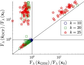
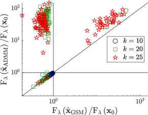
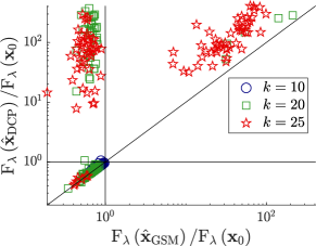
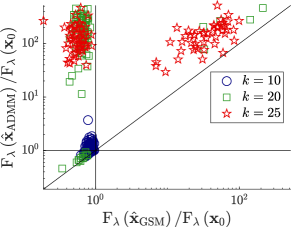
We considered the following simulation setup: In each realization, we generate a random matrix $A$ of size $60\times 300$ whose entries are i.i.d. $\mathcal{N}{\left({0,1}\right)}$, followed by column normalization. For $k\in{\left\{{10,20,25}\right\}}$, we generate a random $k$-sparse signal $\mbox{\boldmath$x$}_{0}$ whose nonzero coordinates are i.i.d. $\mathcal{N}{\left({0,1}\right)}$. We observe $\mbox{\boldmath$y$}=A\mbox{\boldmath$x$}_{0}+\mbox{\boldmath$e$}$, where $\mbox{\boldmath$e$}\in\mathbb{R}^{60}$ is a random noise vector whose entries are i.i.d. $\mathcal{N}{\left({0,1}\right)}$, normalized such that ${\left\|{\mbox{\boldmath$e$}}\right\|}_{2}=0.01\cdot{\left\|{A\mbox{\boldmath$x$}_{0}}\right\|}_{2}$. We considered several values of $\lambda$ in the interval $[10^{-5},1]\cdot{\bar{\lambda}}$, where ${\bar{\lambda}}$ is defined in Equation 2.1. For each obtained solution $\hat{\mbox{\boldmath$x$}}$, we compute its normalized objective ${\mathrm{F}_{\lambda}}{\left({\mbox{\boldmath$\hat{\mbox{\boldmath$x$}}$}}\right)}/{\mathrm{F}_{\lambda}}{\left({\mbox{\boldmath$x$}_{0}}\right)}$. Values near or below $1$ indicate solutions close to the global minimizer, as follows from Theorem 2.5, whereas values significantly above $1$ indicate highly suboptimal solutions, typically with a very different support from that of $\mbox{\boldmath$x$}_{0}$.

Figure 1 shows, for two different values of $\lambda$, the normalized objectives obtained by the three methods for 100 random realizations. Points above the diagonal represent instances for which GSM found solutions with lower objective values than the competing method. As seen in the figure, small values of $k$ lead to relatively easy problems, where all methods succeed. At larger values of $k$, a significant number of instances are in the top left quadrant, which represent instances where DC-programming and ADMM found highly-suboptimal solutions in comparison to those found by GSM. Similar results were obtained for other values of $\lambda$.

(a) $\lambda=0.005\cdot{\bar{\lambda}}$

(b) $\lambda=0.005\cdot{\bar{\lambda}}$

(c) $\lambda=0.5\cdot{\bar{\lambda}}$

(d) $\lambda=0.5\cdot{\bar{\lambda}}$

Figure 1: Objective values of solutions to Equation 1.3 obtained by DC programming (left) and by ADMM (right), compared with the objective of the solution obtained by our GSM method. Each objective value is normalized by that of the original $\mbox{\boldmath$x$}_{0}$. Each point represents one realization. Points above the diagonal represent instances where GSM found better solutions. Normalized objectives much higher than $1$ indicate highly suboptimal solutions.

5.2 Sparse signal recovery

Next, we compare the performance of GSM to several popular methods in sparse signal recovery. We observe $\mbox{\boldmath$y$}=A\mbox{\boldmath$x$}_{0}+\mbox{\boldmath$e$}$, where the $k$-sparse signal $\mbox{\boldmath$x$}_{0}\in{\mathbb{R}^{d}}$, matrix $A\in{\mathbb{R}^{n\times d}}$ and noise vector $\mbox{\boldmath$e$}\in{\mathbb{R}^{n}}$ were generated as described below.

We considered two types of random matrices $A$: Uncorrelated matrices, whose entries are i.i.d. $\mathcal{N}(0,1)$, and correlated matrices, whose rows are drawn from a $d$-dimensional Gaussian distribution $\mathcal{N}{\left({{\bf 0},\Sigma}\right)}$, with covariance matrix $\Sigma$ given by $\sigma_{i,j}=\rho^{{\left|{i-j}\right|}}$, $\rho=0.8$, similarly to [bertsimas2016best]. In both cases, the columns of $A$ were normalized to have unit $\ell_{2}$-norm. Three types of signals $\mbox{\boldmath$x$}_{0}$ were used: (i) Gaussian, whose $k$ nonzero entries are at randomly chosen indices and their values are i.i.d. $\mathcal{N}(0,1)$; (ii) equispaced linear, whose $k$ nonzeros are at equispaced indices, their magnitudes are chosen from $\left\{{1+\frac{i-1}{k-1}29}\,\middle|\,{i=1,\ldots,k}\right\}$ randomly without repetition, and their signs are i.i.d. $\pm 1$; (iii) equispaced $\pm 1$, similar to (ii) only that the nonzero entries are i.i.d. $\pm 1$. Similar simulation designs were considered, e.g., in [buhlmann2013correlated].

The vector $\mbox{\boldmath$e$}\in{\mathbb{R}^{n}}$ is drawn from $\mathcal{N}({\bf 0},\sigma^{2}I_{n})$ with variance $\sigma^{2}{\ =\ }\nu^{2}\mathbb{E}_{\mbox{\boldmath$x$}}{\left[{{\left\|{A\mbox{\boldmath$x$}}\right\|}_{2}^{2}}\right]}/n$, where $\nu\in{\left[{0,1}\right]}$ is a noise-strength parameter, and the expectation $\mathbb{E}_{\mbox{\boldmath$x$}}{\left[{{\left\|{A\mbox{\boldmath$x$}}\right\|}_{2}^{2}}\right]}$ is over the distribution of $\mbox{\boldmath$x$}_{0}$, estimated empirically from 2000 randomly drawn signals. With these definitions, the signal-to-noise ratio (SNR) is given by $\mbox{SNR}=\mathbb{E}_{\mbox{\boldmath$x$}}{\left[{\|A\mbox{\boldmath$x$}\|_{2}^{2}}\right]}/\mathbb{E}_{\mbox{\boldmath$e$}}{\left[{\|\mbox{\boldmath$e$}\|_{2}^{2}}\right]}=1/\nu^{2}$.

Evaluated methods

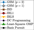
We compared the following 8 methods: 1-2) Two variants of our GSM, with residual norm power $p=2$ or $p=1$, as in Equations 1.3 and 1.4 respectively; 3) Iterative support detection (ISD) [wang2010sparse]; 4-5) $\ell_{p}$-minimization by IRLS or by IRL1; 6) Minimization of the trimmed lasso by DC programming [bertsimas2017trimmed, algorithm 1]; 7) Least-squares OMP; 8) Basis pursuit denoising [chen2001atomic]. For ISD, we used the code provided by its authors. For all other methods, we used our own Matlab implementation. As we assume that the sparsity level $k$ is given, the output of each method was post-processed by solving a least-squares problem on its $k$ largest-magnitude entries and setting the other entries to zero — thereby ensuring that the evaluated solution is $k$-sparse and is optimal on its support. Further technical details appear in Appendix E.

Performance evaluation

A solution $\hat{\mbox{\boldmath$x$}}$ is evaluated by the following 3 quality measures: (i) normalized objective value; (ii) relative recovery error, and (iii) support precision, given by

$$\text{NormObj}{\left({\mbox{\boldmath$\hat{\mbox{\boldmath$x$}}$}}\right)}{\ =\ }\frac{{\left\|{A\mbox{\boldmath$\hat{\mbox{\boldmath$x$}}$}-\mbox{\boldmath$y$}}\right\|}_{2}}{{\left\|{A\mbox{\boldmath$x$}_{0}-\mbox{\boldmath$y$}}\right\|}_{2}},\ \text{RecErr}{\left({\mbox{\boldmath$\hat{\mbox{\boldmath$x$}}$}}\right)}{\ =\ }\frac{{\left\|{\mbox{\boldmath$\hat{\mbox{\boldmath$x$}}$}-\mbox{\boldmath$x$}_{0}}\right\|}_{1}}{{\left\|{\mbox{\boldmath$x$}_{0}}\right\|}_{1}},\ \text{SuppPrec}{\left({\mbox{\boldmath$\hat{\mbox{\boldmath$x$}}$}}\right)}{\ =\ }\frac{{\left|{\text{supp}{\left({\mbox{\boldmath$\hat{\mbox{\boldmath$x$}}$}}\right)}\cap\text{supp}{\left({\mbox{\boldmath$x$}_{0}}\right)}}\right|}}{k}$$

where $\text{supp}{\left({\mbox{\boldmath$x$}}\right)}=\left\{{i\in{\left[{d}\right]}}\,\middle|\,{x_{i}\neq 0}\right\}$. An optimization is deemed successful if $\text{NormObj}{\left({\mbox{\boldmath$\hat{\mbox{\boldmath$x$}}$}}\right)}\leq 1$. Such solutions $\hat{\mbox{\boldmath$x$}}$ are guaranteed by Theorem 2.6 to be close to the ground-truth $\mbox{\boldmath$x$}_{0}$, provided that ${\alpha_{2k}}$ is not too small. In contrast, solutions with $\text{NormObj}{\left({\mbox{\boldmath$\hat{\mbox{\boldmath$x$}}$}}\right)}\gg 1$ are highly suboptimal, and are often poor estimates of $\mbox{\boldmath$x$}_{0}$. We consider a recovery successful if $\text{RecErr}{\left({\mbox{\boldmath$\hat{\mbox{\boldmath$x$}}$}}\right)}\leq\max\{2\nu,10^{-3}\}$. The additional threshold of $10^{-3}$ is needed to accommodate methods that have early stopping criteria. The results are not sensitive to these specific thresholds.

Recovery performance as a function of sparsity level

For each $k\in{\left\{{16,18,20,\ldots,48}\right\}}$ we generated 200 random instances of $A$,$\mbox{\boldmath$x$}_{0}$ and $e$, with $A\in{\mathbb{R}^{100\times 800}}$ and essentially zero noise ($\nu=10^{-6}$). The results of the eight methods appear in Figure 2. As seen in the plots, GSM achieved the highest optimization and recovery success rates, with the closest competitor being ISD. The improved performance of ISD over some of the other methods is in accordance with [wang2010sparse]. Empirically, the power-2 variant of GSM was slightly better than the power-1 variant. GSM also achieved the best average support precision, except at large values of $k$, where the recovery success rates of all methods were near zero.

Figure 2: Recovery of $k$-sparse signals in a near-zero noise setting ($\nu=10^{-6}$). Matrix size: $100\times 800$. Top row: Gaussian signal, uncorrelated matrix. Bottom row: Equispaced linear signal, correlated matrix.

Figure 3: Recovery of $k$-sparse signals in a $\nu=5\%$ noise setting. Top row: Gaussian signal, uncorrelated matrix. Bottom row: Equispaced linear signal, correlated matrix.

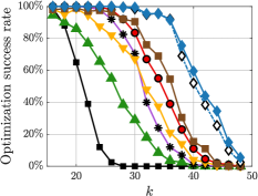
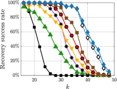
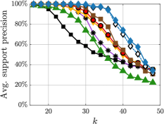
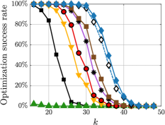
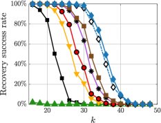
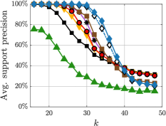
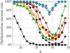
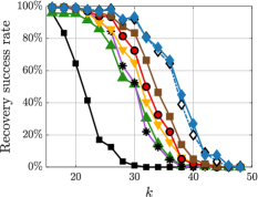
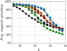
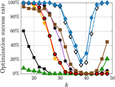
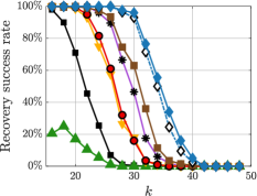
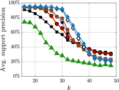
Figure 3 shows the results under 5% noise ($\nu=0.05$). Even though noise degraded the performance of all methods, GSM achieved the highest accuracy. In contrast to the noiseless case, here at high values of $k$, some methods obtain a small residual $\|A\mbox{\boldmath$x$}-\mbox{\boldmath$y$}\|_{2}$ by an incorrect set of columns, whose linear combination overfits the noisy vector $y$ – hence the notable difference between the optimization and recovery success rates. Further results appear in Appendix A. Similar qualitative results (not shown) were obtained with $50\times 1000$ matrices.

Number of required measurements

Next, we compare the number of measurements $n$ required for successful recovery in a noiseless setting by GSM and by the next best competitor, ISD, under the same setup as in [wang2010sparse, Figures 3-5]. Specifically, for $d=600$, we generate a $k$-sparse vector $\mbox{\boldmath$x$}_{0}$ whose non-zero entries are i.i.d. $\mathcal{N}{\left({0,1}\right)}$, where $k\in\{8,40,150\}$. Then, for various values of $n$, we estimate $\mbox{\boldmath$x$}_{0}$ from $\mbox{\boldmath$y$}=A\mbox{\boldmath$x$}_{0}$, where $A\in{\mathbb{R}^{n\times d}}$ has i.i.d. entries $\mathcal{N}{\left({0,1}\right)}$ without column normalization. A recovery is considered successful if $\|\hat{}\mbox{\boldmath$x$}-\mbox{\boldmath$x$}_{0}\|_{1}/\|\mbox{\boldmath$x$}_{0}\|_{1}<10^{-4}$. Figure 4 illustrates the recovery success rates over 100 instances for each $n$, with GSM able to successfully recover a sparse signal from fewer measurements than ISD.

Figure 4: Recovery success rate of GSM and ISD for a $k$-sparse Gaussian signal in ${\mathbb{R}^{d}}$, with $d=600$, as a function of the number of measurements $n$.

5.3 Comparison with MIP-based methods

Finally, we compare the power-2 variant of GSM with two recent mixed integer programming based approaches, considered state-of-the-art in solving (P0): (1) The cutting plane method [bertsimas2020sparse], and (2) the coordinate descent and local combinatorial search method [hazimeh2020fast]. We did not run the first method ourselves but rather, as described below, compare our results to those reported in their work, under identical settings. We ran the second method using the authors’ L0learn R package. We tested it both with and without local combinatorial search, denoted by CD+Comb and CD, respectively.

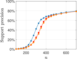
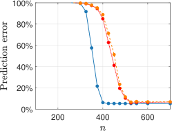
First, we replicate the two settings of Figure 2(right) and Figure 4(left) in [bertsimas2020sparse]. Specifically, for varying values of $n$, we generate an $n\times d$ matrix $A$ with uncorrelated i.i.d. entries $\mathcal{N}{\left({0,1}\right)}$ without column normalization. We then generate a $k$-sparse vector $\mbox{\boldmath$x$}_{0}\in{\mathbb{R}^{d}}$ with $k=10$, whose nonzero entries are chosen randomly from $\pm 1$ and placed at random indices. We observe $\mbox{\boldmath$y$}=A\mbox{\boldmath$x$}_{0}+\mbox{\boldmath$e$}$ where $e$ has i.i.d. $\mathcal{N}{\left({0,1}\right)}$ entries, normalized such that $\textup{SNR}=1/\nu^{2}={\left\|{A\mbox{\boldmath$x$}_{0}}\right\|}^{2}_{2}/{\left\|{\mbox{\boldmath$e$}}\right\|}^{2}_{2}$. We considered the following two settings as in [bertsimas2020sparse]: (a) $d=15000$, SNR=400; and (b) $d=5000$, SNR=9. Both the cutting plane method and our GSM received as input the correct value of $k$. In contrast, the coordinate descent method, returns a set of solutions with different sparsity levels. We gave their method a slight advantage by choosing the solution whose support $\hat{S}$ is the closest to the ground-truth support $S_{0}$ in terms of the F-score: $2\frac{{\left|{\hat{S}\cap S_{0}}\right|}}{{\left|{\hat{S}}\right|}+{\left|{S_{0}}\right|}}$.

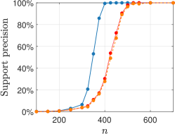
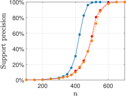
As in [bertsimas2020sparse], we measure the quality of a solution $\hat{\mbox{\boldmath$x$}}$ by its support precision, ${\left|{\hat{S}\cap S_{0}}\right|}/k$. Figure 5 compares the performance of GSM, CD and CD+Comb, averaged over 200 random instances for each value of $n$. To achieve a precision comparable to GSM, CD+Comb required about $20\%$ more observations. In terms of run-time, our method, implemented in Matlab, took on average less than 3 minutes to complete a single run. The CD/CD+Comb method, partly implemented in C++, is significantly faster and took less than 1 second per run.

Given the NP-hardness of (P0), in their original paper, [bertsimas2020sparse] did not run their exact cutting plane method till it found the optimal solution, but rather capped each run to at most 10 minutes. With this time limit, their performance was much worse than that of GSM. For example, in setting (a) they achieved an average support precision smaller than 30% at $n=100$. In comparison, our GSM achieved an 88% precision.

(a) $d=15000$, $\textup{SNR}=400$

(b) $d=5000$, $\textup{SNR}=9$

Figure 5: Support precision in recovering a $k$-sparse signal, $k=10$, with an uncorrelated matrix ($\rho=0$). Settings (a) and (b) correspond to Figure 2(right) and Figure 4(left) in [bertsimas2020sparse].

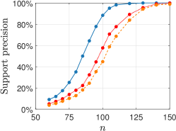
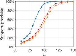
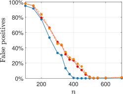
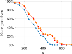
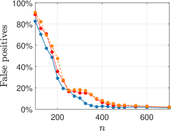
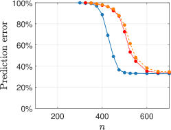
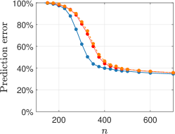
Finally, to highlight the performance achievable by GSM versus that of CD/CD+Comb, we considered the following quite challenging setup: For $d=20000$, $k=50$ and varying values of $n$, a $n\times d$ Gaussian matrix $A$ was generated with correlated columns, with coefficient $\rho=0.5$. The observed vector $\mbox{\boldmath$y$}=A\mbox{\boldmath$x$}_{0}+\mbox{\boldmath$e$}$ was generated with random Gaussian noise $e$. Here we followed the definition of SNR of [hazimeh2020fast], and normalized $e$ such that $\textup{SNR}=1/\nu^{2}=\mathbb{E}_{A}{\left[{{\left\|{A\mbox{\boldmath$x$}_{0}}\right\|}^{2}_{2}}\right]}/\mathbb{E}_{\mbox{\boldmath$e$}}{\left[{{\left\|{\mbox{\boldmath$e$}}\right\|}^{2}_{2}}\right]}$. Three different settings were tested: (a) $\mbox{\boldmath$x$}_{0}$ equispaced $\pm 1$, SNR=400; (b) $\mbox{\boldmath$x$}_{0}$ equispaced $\pm 1$, SNR=9; and (c) $\mbox{\boldmath$x$}_{0}$ equispaced linear, SNR=9.

In these simulations, the true sparsity level $k$ was unknown. As in [hazimeh2020fast], we also observe a separate random design validation set of the same size, $\tilde{\mbox{\boldmath$y$}}=\tilde{A}\mbox{\boldmath$x$}_{0}+\tilde{\mbox{\boldmath$e$}}$. We ran our GSM method for input sparsity $k\in[1,60]$, and choose the solution with smallest prediction error on the validation set. For CD/CD+Comb, we passed the ground-truth $k$ as an upper limit on the support size, and similarly took the solution with smallest validation prediction error.

Similar to [hazimeh2020fast], we also calculated the false positive rate $\frac{{\left|{\hat{S}\cap S_{0}^{c}}\right|}}{{\left|{\hat{S}}\right|}}$ and the expected prediction error $\frac{\mathbb{E}_{A}{\left[{{\left\|{A\mbox{\boldmath$\hat{\mbox{\boldmath$x$}}$}-\mbox{\boldmath$y$}}\right\|}_{2}^{2}}\right]}}{\mathbb{E}_{A}{\left[{{\left\|{\mbox{\boldmath$y$}}\right\|}_{2}^{2}}\right]}}$. Figure 6 shows the results, averaged over 100 instances for each $n$. As seen in the individual plots, GSM achieved superior recovery. The runtime of our method was approximately 10 minutes for each combination of $n,k$.

(a)

(b)

(c)

(d)

(e)

(f)

(g) $\textup{SNR}=400$, entries $\pm 1$

(h) $\textup{SNR}=9$, entries $\pm 1$

(i) $\textup{SNR}=9$, linear magnitudes

Figure 6: Sparse signal recovery with $d=20000$, $k=50$ and correlation parameter $\rho=0.5$. Top to bottom: Support precision, false positive rate, prediction error. The vectors in the left and center columns are with nonzero entries $\pm 1$. In the right column, the nonzeros are with linear magnitudes.

Summary

Via several simulations, we illustrated the competitive performance of GSM in solving Equation P0 and recovering sparse signals. This improved performance, nonetheless, comes at a computational cost. Each run of GSM typically considered up to 30 different values of $\lambda$. For each $\lambda$, solving Equation 1.3 by homotopy required several hundreds of values of $\gamma$. For each $\gamma$, solving Equation 3.5 often took three MM iterations. Hence, one run of GSM solved several thousands of weighted $\ell_{1}$ problems Equation 3.15 or Equation 3.16. We remark that optimizations of Equation 1.3 over different values of $\lambda$ can be done in parallel. Further speedups may be possible by using specialized weighted $\ell_{1}$ solvers that can be warm-started at the solutions of previous problem instances.

Appendix A Further numerical results

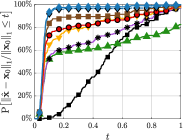
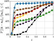
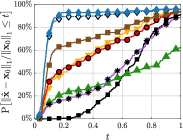
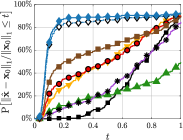
To further illustrate the improved performance of GSM, fig. 7 shows, for selected values of $k$, the cumulative distribution of the normalized recovery error

$$\mbox{G}(t)=\mbox{P}{\left[{\|\hat{}\mbox{\boldmath$x$}-\mbox{\boldmath$x$}_{0}\|_{1}/\|\mbox{\boldmath$x$}_{0}\|_{1}\leq t}\right]}$$

under 5% noise ($\nu=0.05$). These results show that the better success rates of GSM are not sensitive to the specific threshold that defines a successful recovery.

(a) $k=30$

(b) $k=32$

(c) $k=34$

(d) $k=36$

(e)

Figure 7: Cumulative distribution of the relative recovery error ${\left\|{\mbox{\boldmath$\hat{\mbox{\boldmath$x$}}$}-\mbox{\boldmath$x$}_{0}}\right\|}_{1}/{\left\|{\mbox{\boldmath$x$}_{0}}\right\|}_{1}$ under 5% noise ($\nu=0.05$). Gaussian signal, uncorrelated $100\times 800$ matrix.

Appendix B Proofs

B.1 Theory for the trimmed lasso

In our proofs, we shall use the following inequality

$${}\begin{split}{\left\|{A\mbox{\boldmath$v$}}\right\|}_{2}\leq{\lambda_{b}}{\left\|{\mbox{\boldmath$v$}}\right\|}_{1}\qquad\forall\mbox{\boldmath$v$}\in{\mathbb{R}^{d}},\end{split}$$ (B.1)

where ${\lambda_{b}}$ is as in Equation 2.2. This inequality follows directly from the triangle inequality.

Proof of Theorem 2.1.

Let ${\mbox{\boldmath$x$}^{*}}$ be a local minimum of ${\mathrm{F}_{\lambda}}$. Let $\Lambda\subset{\left[{d}\right]}$ be an index set of the $d-k$ smallest-magnitude entries of ${\mbox{\boldmath$x$}^{*}}$, breaking ties arbitrarily. Define $\mathbf{w}\in{\mathbb{R}^{d}}$ by

$$\begin{split}w_{i}=\left\{\begin{array}[]{lc}1&i\in\Lambda\\ 0&\mbox{otherwise.}\end{array}\right.\end{split}$$

Let ${\mathrm{F}_{\lambda,\mathbf{w}}}(\mbox{\boldmath$x$}){\ =\ }\frac{1}{2}{\left\|{A\mbox{\boldmath$x$}-\mbox{\boldmath$y$}}\right\|}_{2}^{2}+\lambda{{\left<{{\mathbf{w}},\ {{\left|{\mbox{\boldmath$x$}}\right|}}}\right>}}.$ Then ${\mathrm{F}_{\lambda}}{\left({{\mbox{\boldmath$x$}^{*}}}\right)}={\mathrm{F}_{\lambda,\mathbf{w}}}{\left({{\mbox{\boldmath$x$}^{*}}}\right)}$. Moreover, for any $\mbox{\boldmath$x$}\in{\mathbb{R}^{d}}$, ${\mathrm{F}_{\lambda}}{\left({\mbox{\boldmath$x$}}\right)}\leq{\mathrm{F}_{\lambda,\mathbf{w}}}{\left({\mbox{\boldmath$x$}}\right)}$. Hence, the assumption that ${\mbox{\boldmath$x$}^{*}}$ is a local minimum of ${\mathrm{F}_{\lambda}}$ implies that ${\mbox{\boldmath$x$}^{*}}$ is also a local minimum of ${\mathrm{F}_{\lambda,\mathbf{w}}}$. Since ${\mathrm{F}_{\lambda,\mathbf{w}}}$ is convex, then ${\mbox{\boldmath$x$}^{*}}$ is also a global minimum.

Next, we claim that ${\left\|{A{\mbox{\boldmath$x$}^{*}}-\mbox{\boldmath$y$}}\right\|}_{2}\leq{\left\|{\mbox{\boldmath$y$}}\right\|}_{2}$. Suppose otherwise by contradiction. Note that ${{\left<{{\mathbf{w}},\ {{\left|{{\mbox{\boldmath$x$}^{*}}}\right|}}}\right>}}\geq 0={{\left<{{\mathbf{w}},\ {{\left|{{\bf 0}}\right|}}}\right>}}$. Thus,

$$\begin{split}{\mathrm{F}_{\lambda,\mathbf{w}}}{\left({{\mbox{\boldmath$x$}^{*}}}\right)}&=\tfrac{1}{2}{\left\|{A{\mbox{\boldmath$x$}^{*}}-\mbox{\boldmath$y$}}\right\|}_{2}^{2}+\lambda{{\left<{{\mathbf{w}},\ {{\left|{{\mbox{\boldmath$x$}^{*}}}\right|}}}\right>}}\\ &>\tfrac{1}{2}{\left\|{\mbox{\boldmath$y$}}\right\|}_{2}^{2}+\lambda{{\left<{{\mathbf{w}},\ {{\left|{{\mbox{\boldmath$x$}^{*}}}\right|}}}\right>}}\geq\tfrac{1}{2}{\left\|{\mbox{\boldmath$y$}}\right\|}_{2}^{2}+\lambda{{\left<{{\mathbf{w}},\ {{\left|{{\bf 0}}\right|}}}\right>}}={\mathrm{F}_{\lambda,\mathbf{w}}}{\left({{\bf 0}}\right)},\end{split}$$

contradicting the fact that ${\mbox{\boldmath$x$}^{*}}$ is a global minimum of ${\mathrm{F}_{\lambda,\mathbf{w}}}$.

For a function $f:{\mathbb{R}^{d}}\rightarrow{\mathbb{R}}$, denote by $\partial f(\mbox{\boldmath$x$})$ the subdifferential of $f$ at $x$. We now calculate $\partial{\mathrm{F}_{\lambda,\mathbf{w}}}({\mbox{\boldmath$x$}^{*}})$. The term $\frac{1}{2}{\left\|{A\mbox{\boldmath$x$}-\mbox{\boldmath$y$}}\right\|}^{2}_{2}$ is differentiable everywhere, and its subdifferential at $x$ is the singleton containing its gradient ${\left\{{A^{T}{\left({A\mbox{\boldmath$x$}-\mbox{\boldmath$y$}}\right)}}\right\}}$. Next, define for $\mbox{\boldmath$x$}\in{\mathbb{R}^{d}}$,

$$V(\mbox{\boldmath$x$})=\left\{{\mbox{\boldmath$v$}\in{\mathbb{R}^{d}}}\,\middle|\,{{\left\|{\mbox{\boldmath$v$}}\right\|}_{\infty}\leq 1,\mbox{ and }\forall i\mbox{ with }x_{i}\neq 0,v_{i}=\operatorname*{sign}{x_{i}}}\right\}.$$ (B.2)

It can be shown that the subdifferential of ${{\left<{{\mathbf{w}},\ {{\left|{\mbox{\boldmath$x$}}\right|}}}\right>}}$ at $x$ is given by the following set

$$\begin{split}\partial{{\left<{{\mathbf{w}},\ {{\left|{\mbox{\boldmath$x$}}\right|}}}\right>}}=\left\{{\mbox{\boldmath$v$}{\odot}\mathbf{w}}\,\middle|\,{\mbox{\boldmath$v$}\in V(\mbox{\boldmath$x$})}\right\},\end{split}$$

where ${\odot}$ denotes the Hadamard (entrywise) product. Therefore, by the Moreau-Rockafellar theorem on the additivity of subdifferentials [bertsekas2003convanal, Prop. 4.2.4, pg. 232][balder2010subdiff, Thm. 2.9],

$$\begin{split}\partial{\mathrm{F}_{\lambda,\mathbf{w}}}(\mbox{\boldmath$x$})=\left\{{A^{T}{\left({A\mbox{\boldmath$x$}-\mbox{\boldmath$y$}}\right)}+\lambda\mbox{\boldmath$v$}{\odot}\mathbf{w}}\,\middle|\,{\mbox{\boldmath$v$}\in V(\mbox{\boldmath$x$})}\right\}.\end{split}$$

Since ${\mbox{\boldmath$x$}^{*}}$ is a global minimum of ${\mathrm{F}_{\lambda,\mathbf{w}}}$, $\partial{\mathrm{F}_{\lambda,\mathbf{w}}}({\mbox{\boldmath$x$}^{*}})$ contains the zero vector. Thus, there exists $\mbox{\boldmath$v$}\in V({\mbox{\boldmath$x$}^{*}})$ such that $A^{T}{\left({A{\mbox{\boldmath$x$}^{*}}-\mbox{\boldmath$y$}}\right)}+\lambda\mbox{\boldmath$v$}{\odot}\mathbf{w}={\bf 0}.$

Suppose that ${\mbox{\boldmath$x$}^{*}}$ is not $k$-sparse. Then there exists some index $i$ such that $w_{i}=1$ and $x^{*}_{i}\neq 0$. At that index $i$, ${{\left<{{\mbox{\boldmath$a$}_{i}},\ {A{\mbox{\boldmath$x$}^{*}}-\mbox{\boldmath$y$}}}\right>}}+\lambda\cdot\operatorname*{sign}{x^{*}_{i}}=0$. Since ${\left\|{A{\mbox{\boldmath$x$}^{*}}-\mbox{\boldmath$y$}}\right\|}_{2}\leq{\left\|{\mbox{\boldmath$y$}}\right\|}_{2}$,

$$\begin{split}\lambda={\left|{{{\left<{{\mbox{\boldmath$a$}_{i}},\ {A{\mbox{\boldmath$x$}^{*}}-\mbox{\boldmath$y$}}}\right>}}}\right|}\leq{\left\|{\mbox{\boldmath$a$}_{i}}\right\|}_{2}{\left\|{A{\mbox{\boldmath$x$}^{*}}-\mbox{\boldmath$y$}}\right\|}_{2}\leq{\left\|{\mbox{\boldmath$a$}_{i}}\right\|}_{2}{\left\|{\mbox{\boldmath$y$}}\right\|}_{2}\leq\max_{j=1,\ldots,d}{\left\|{\mbox{\boldmath$a$}_{j}}\right\|}_{2}{\left\|{\mbox{\boldmath$y$}}\right\|}_{2}=\bar{\lambda}.\end{split}$$

Hence, for any $\lambda>\bar{\lambda}$ any local minimum of ${\mathrm{F}_{\lambda}}$ must be $k$-sparse. ∎

Proof of Theorem 2.2.

Let ${\mbox{\boldmath$x$}^{*}}$ be a local minimum of ${\mathrm{F}^{1}_{\lambda}}$, where $\lambda>{\lambda_{b}}$. Suppose by contradiction that ${\mbox{\boldmath$x$}^{*}}$ is not $k$-sparse. Let $\mbox{\boldmath$v$}{\ =\ }{\Pi_{k}}{\left({{\mbox{\boldmath$x$}^{*}}}\right)}-{\mbox{\boldmath$x$}^{*}}\neq{\bf 0}$. Then for any $t\in{\left[{0,1}\right]}$,

$$\begin{split}{\mathrm{F}^{1}_{\lambda}}{\left({{\mbox{\boldmath$x$}^{*}}+t\mbox{\boldmath$v$}}\right)}-{\mathrm{F}^{1}_{\lambda}}({\mbox{\boldmath$x$}^{*}})={\left\|{A{\left({{\mbox{\boldmath$x$}^{*}}+t\mbox{\boldmath$v$}}\right)}-\mbox{\boldmath$y$}}\right\|}_{2}-{\left\|{A{\mbox{\boldmath$x$}^{*}}-\mbox{\boldmath$y$}}\right\|}_{2}+\lambda{\left[{{{\tau}_{k}}{\left({{\mbox{\boldmath$x$}^{*}}+t\mbox{\boldmath$v$}}\right)}-{{\tau}_{k}}({\mbox{\boldmath$x$}^{*}})}\right]}.\end{split}$$

By the triangle inequality,

$$\begin{split}{\left\|{A{\left({{\mbox{\boldmath$x$}^{*}}+t\mbox{\boldmath$v$}}\right)}-\mbox{\boldmath$y$}}\right\|}_{2}-{\left\|{A{\mbox{\boldmath$x$}^{*}}-\mbox{\boldmath$y$}}\right\|}_{2}\leq t{\left\|{A\mbox{\boldmath$v$}}\right\|}_{2}.\end{split}$$

As for the second term, ${{\mbox{\boldmath$x$}^{*}}+t\mbox{\boldmath$v$}}={{\left({1-t}\right)}{\mbox{\boldmath$x$}^{*}}+t{\Pi_{k}}{\left({{\mbox{\boldmath$x$}^{*}}}\right)}}$. This vector coincides with ${\mbox{\boldmath$x$}^{*}}$ on the $k$ largest-magnitude entries of ${\mbox{\boldmath$x$}^{*}}$, and its remaining entries decrease linearly in magnitude with ${\left({1-t}\right)}$. Therefore, ${{\tau}_{k}}{\left({{\mbox{\boldmath$x$}^{*}}+t\mbox{\boldmath$v$}}\right)}=(1-t){{\tau}_{k}}({\mbox{\boldmath$x$}^{*}}).$ Furthermore, since ${{\tau}_{k}}({\mbox{\boldmath$x$}^{*}})={\left\|{\mbox{\boldmath$v$}}\right\|}_{1}$

$$\begin{split}{\mathrm{F}^{1}_{\lambda}}{\left({{\mbox{\boldmath$x$}^{*}}+t\mbox{\boldmath$v$}}\right)}-{\mathrm{F}^{1}_{\lambda}}({\mbox{\boldmath$x$}^{*}})\leq t{\left\|{A\mbox{\boldmath$v$}}\right\|}_{2}+\lambda{\left[{{\left({1-t}\right)}{{\tau}_{k}}{\left({{\mbox{\boldmath$x$}^{*}}}\right)}-{{\tau}_{k}}({\mbox{\boldmath$x$}^{*}})}\right]}=t\left({\left\|{A\mbox{\boldmath$v$}}\right\|}_{2}-\lambda{\left\|{\mbox{\boldmath$v$}}\right\|}_{1}\right).\end{split}$$

By Eqs. Equation B.1, Equation 2.2 and the fact that ${\left\|{\mbox{\boldmath$v$}}\right\|}_{1}{\left({{\lambda_{b}}-\lambda}\right)}<0$, for all $t\in\left(0,1\right]$,

$$\begin{split}{\mathrm{F}^{1}_{\lambda}}{\left({{\mbox{\boldmath$x$}^{*}}+t\mbox{\boldmath$v$}}\right)}-{\mathrm{F}^{1}_{\lambda}}({\mbox{\boldmath$x$}^{*}})\leq t{\left\|{\mbox{\boldmath$v$}}\right\|}_{1}{\left({{\lambda_{b}}-\lambda}\right)}<0.\end{split}$$

This contradicts the assumption that ${\mbox{\boldmath$x$}^{*}}$ is a local minimum of ${\mathrm{F}^{1}_{\lambda}}$. ∎

To prove Theorem 2.3, we first state and prove the following auxiliary lemma.

Lemma B.1.

Suppose the matrix $A\in{\mathbb{R}^{n\times d}}$ is of rank $n$, so that ${\lambda_{a}}>0$. Let $\mathbf{w}\in{\left[{0,1}\right]}^{d}$ such that $\sum_{i=1}^{d}w_{i}=d-k$. Let ${\mbox{\boldmath$x$}^{*}}$ be a global minimum of

$$\begin{split}{\mathrm{F}^{1}_{\lambda,\mathbf{w}}}(\mbox{\boldmath$x$}){\ =\ }{\left\|{A\mbox{\boldmath$x$}-\mbox{\boldmath$y$}}\right\|}_{2}+\lambda{{\left<{{\mathbf{w}},\ {{\left|{\mbox{\boldmath$x$}}\right|}}}\right>}},\end{split}$$

where $0<\lambda<{\lambda_{a}}$. Then $A{\mbox{\boldmath$x$}^{*}}=\mbox{\boldmath$y$}$.

Proof.

Suppose by contradiction that $A{\mbox{\boldmath$x$}^{*}}\neq\mbox{\boldmath$y$}$. Let $\partial{\mathrm{F}^{1}_{\lambda,\mathbf{w}}}(\mbox{\boldmath$x$})$ denote the subdifferential of ${\mathrm{F}^{1}_{\lambda,\mathbf{w}}}$ at $x$. Since $A{\mbox{\boldmath$x$}^{*}}\neq\mbox{\boldmath$y$}$, the term ${\left\|{A\mbox{\boldmath$x$}-\mbox{\boldmath$y$}}\right\|}_{2}$ is differentiable at $\mbox{\boldmath$x$}={\mbox{\boldmath$x$}^{*}}$, and its subdifferential at ${\mbox{\boldmath$x$}^{*}}$ is a singleton consisting of its gradient, namely

$$\begin{split}{\phantom{\bigg{\lvert}}{\partial{\left\|{A\mbox{\boldmath$x$}-\mbox{\boldmath$y$}}\right\|}_{2}}\bigg{\rvert}_{\mbox{\boldmath$x$}={\mbox{\boldmath$x$}^{*}}}}={\left\{{A^{T}\frac{A{\mbox{\boldmath$x$}^{*}}-\mbox{\boldmath$y$}}{{\left\|{A{\mbox{\boldmath$x$}^{*}}-\mbox{\boldmath$y$}}\right\|}_{2}}}\right\}}.\end{split}$$

The subdifferential of ${{\left<{{\mathbf{w}},\ {{\left|{\mbox{\boldmath$x$}}\right|}}}\right>}}$ at $x$ is given by $\partial{{\left<{{\mathbf{w}},\ {{\left|{\mbox{\boldmath$x$}}\right|}}}\right>}}=\left\{{\mbox{\boldmath$v$}{\odot}\mathbf{w}}\,\middle|\,{\mbox{\boldmath$v$}\in V(\mbox{\boldmath$x$})}\right\}$, where $V(\mbox{\boldmath$x$})$ is given by Equation B.2. Therefore, by the Moreau-Rockafellar theorem,

$$\begin{split}\partial{\mathrm{F}^{1}_{\lambda,\mathbf{w}}}({\mbox{\boldmath$x$}^{*}})=\left\{{A^{T}\frac{A{\mbox{\boldmath$x$}^{*}}-\mbox{\boldmath$y$}}{{\left\|{A{\mbox{\boldmath$x$}^{*}}-\mbox{\boldmath$y$}}\right\|}_{2}}+\lambda\mbox{\boldmath$v$}{\odot}\mathbf{w}}\,\middle|\,{\mbox{\boldmath$v$}\in V({\mbox{\boldmath$x$}^{*}})}\right\}.\end{split}$$

Since ${\mbox{\boldmath$x$}^{*}}$ is a global minimum of ${\mathrm{F}^{1}_{\lambda,\mathbf{w}}}$, $\partial{\mathrm{F}^{1}_{\lambda,\mathbf{w}}}({\mbox{\boldmath$x$}^{*}})$ contains the zero vector. Thus, there exists some $\mbox{\boldmath$v$}\in V({\mbox{\boldmath$x$}^{*}})$ such that

$$\begin{split}A^{T}\frac{A{\mbox{\boldmath$x$}^{*}}-\mbox{\boldmath$y$}}{{\left\|{A{\mbox{\boldmath$x$}^{*}}-\mbox{\boldmath$y$}}\right\|}_{2}}+\lambda\mbox{\boldmath$v$}{\odot}\mathbf{w}={\bf 0}.\end{split}$$

This implies that

$$\begin{split}\lambda{\left\|{\mbox{\boldmath$v$}{\odot}\mathbf{w}}\right\|}_{2}={\left\|{A^{T}\frac{A{\mbox{\boldmath$x$}^{*}}-\mbox{\boldmath$y$}}{{\left\|{A{\mbox{\boldmath$x$}^{*}}-\mbox{\boldmath$y$}}\right\|}_{2}}}\right\|}_{2}\geq\sigma_{n}{\left({A}\right)}.\end{split}$$

Since ${\left\|{\mbox{\boldmath$v$}}\right\|}_{\infty}\leq 1$, $\mathbf{w}\in{\left[{0,1}\right]}^{d}$ and $\sum_{i=1}^{d}w_{i}=d-k$, we have:

$$\begin{split}{\left\|{\mbox{\boldmath$v$}{\odot}\mathbf{w}}\right\|}_{2}\leq{\left\|{\mathbf{w}}\right\|}_{2}=\sqrt{{\sum_{i=1}^{d}}w_{i}^{2}}\leq\sqrt{{\sum_{i=1}^{d}}w_{i}}=\sqrt{d-k}.\end{split}$$

Therefore $\sigma_{n}{\left({A}\right)}\leq\lambda\sqrt{d-k},$ which contradicts the assumption that $\lambda<{\lambda_{a}}=\frac{\sigma_{n}{\left({A}\right)}}{\sqrt{d-k}}$. ∎

Proof of Theorem 2.3.

Let ${\mbox{\boldmath$x$}^{*}}$ be a local minimum of ${\mathrm{F}^{1}_{\lambda}}$ with $0<\lambda<{\lambda_{a}}$. Let $\mathbf{w}\in{\mathbb{R}^{d}}$ such that $w_{i}=1$ at indices $i$ corresponding to the $d-k$ smallest-magnitude entries of ${\mbox{\boldmath$x$}^{*}}$, breaking ties arbitrarily, and $w_{i}=0$ elsewhere. By similar arguments to those in the proof of Theorem 2.1, ${\mbox{\boldmath$x$}^{*}}$ is a global minimum of ${\mathrm{F}^{1}_{\lambda,\mathbf{w}}}$. Therefore, by Lemma B.1, $A{\mbox{\boldmath$x$}^{*}}=\mbox{\boldmath$y$}$. ∎

Proof of Theorem 2.4.

We prove the theorem for the power-2 objective ${\mathrm{F}_{\lambda}}$. The proof for ${\mathrm{F}^{1}_{\lambda}}$ is similar. Given a set $\Lambda$ of size $k$, we define the following vector $\mathbf{w}\in{\mathbb{R}^{d}}$

$$w_{i}={\left\{\begin{matrix}{0}&{i\in\Lambda}\\[10.0pt] {1}&{i\notin\Lambda.}\end{matrix}\right.}$$

Let ${\mathrm{F}_{\lambda,\mathbf{w}}}(\mbox{\boldmath$x$}){\ =\ }f{\left({\mbox{\boldmath$x$}}\right)}+\lambda{{\left<{{\mathbf{w}},\ {{\left|{\mbox{\boldmath$x$}}\right|}}}\right>}}$, where $f{\left({\mbox{\boldmath$x$}}\right)}=\frac{1}{2}{\left\|{A\mbox{\boldmath$x$}-\mbox{\boldmath$y$}}\right\|}_{2}^{2}$. As in the proof of Theorem 2.1, with $V(\mbox{\boldmath$x$})$ defined in Equation B.2, the subdifferential of ${\mathrm{F}_{\lambda,\mathbf{w}}}{\left({\mbox{\boldmath$x$}}\right)}$ at $x$ is given by

$$\partial{\mathrm{F}_{\lambda,\mathbf{w}}}(\mbox{\boldmath$x$})=\left\{{\nabla f{\left({\mbox{\boldmath$x$}}\right)}+\lambda\mbox{\boldmath$v$}{\odot}\mathbf{w}}\,\middle|\,{\mbox{\boldmath$v$}\in V(\mbox{\boldmath$x$})}\right\}.$$ (B.3)

Let $\tilde{\mbox{\boldmath$x$}}$ be a global minimizer of ${\left\|{A\mbox{\boldmath$x$}-\mbox{\boldmath$y$}}\right\|}_{2}$ over all vectors $\mbox{\boldmath$x$}\in{\mathbb{R}^{d}}$ supported in $\Lambda$. Namely,

$$\mbox{\boldmath$\tilde{\mbox{\boldmath$x$}}$}=\operatorname*{\arg\!\min}_{\mbox{\boldmath$x$}}\ {\left\|{A\mbox{\boldmath$x$}-\mbox{\boldmath$y$}}\right\|}_{2}\quad\mbox{s.t.}\quad\forall i\notin\Lambda\ x_{i}=0.$$ (B.4)

Assume that $\|\mbox{\boldmath$\tilde{\mbox{\boldmath$x$}}$}\|_{0}=k$. We shall now show that $\tilde{\mbox{\boldmath$x$}}$ is a global minimizer of ${\mathrm{F}_{\lambda,\mathbf{w}}}$ for any $\lambda\geq{\bar{\lambda}}$. Define the vector $\tilde{\mbox{\boldmath$v$}}\in{\mathbb{R}^{d}}$ by

$$\tilde{v}_{i}={\left\{\begin{matrix}{\operatorname*{sign}{\left({x_{i}}\right)}}&{i\in\Lambda}\\[10.0pt] {-\tfrac{1}{\lambda}\nabla f{\left({\mbox{\boldmath$\tilde{\mbox{\boldmath$x$}}$}}\right)}_{i}}&{i\notin\Lambda.}\end{matrix}\right.}$$

To show that $\tilde{\mbox{\boldmath$v$}}$ belongs to $V{\left({\mbox{\boldmath$\tilde{\mbox{\boldmath$x$}}$}}\right)}$, it suffices to show that ${\left|{\tfrac{1}{\lambda}\nabla f{\left({\mbox{\boldmath$\tilde{\mbox{\boldmath$x$}}$}}\right)}_{i}}\right|}\leq 1$ for all $i\notin\Lambda$. Let $i\notin\Lambda$ and recall that ${\bf a}_{i}$ is the $i$-th column of $A$. Then

$${\left|{\nabla f{\left({\mbox{\boldmath$\tilde{\mbox{\boldmath$x$}}$}}\right)}_{i}}\right|}={\left|{{{\left<{{{\bf a}_{i}},\ {A\mbox{\boldmath$\tilde{\mbox{\boldmath$x$}}$}-\mbox{\boldmath$y$}}}\right>}}}\right|}\leq{\left\|{{\bf a}_{i}}\right\|}_{2}{\left\|{A\mbox{\boldmath$\tilde{\mbox{\boldmath$x$}}$}-\mbox{\boldmath$y$}}\right\|}_{2}\overset{\text{(a)}}{\leq}{\left\|{{\bf a}_{i}}\right\|}_{2}{\left\|{\mbox{\boldmath$y$}}\right\|}_{2}\overset{\text{(b)}}{\leq}{\bar{\lambda}}\overset{\text{(c)}}{\leq}\lambda,$$

where (a) holds by our choice of $\tilde{\mbox{\boldmath$x$}}$, (b) holds by the definition of ${\bar{\lambda}}$, and (c) holds by the theorem assumption. By definition, $\nabla f{\left({\mbox{\boldmath$\tilde{\mbox{\boldmath$x$}}$}}\right)}+\lambda\tilde{\mbox{\boldmath$v$}}{\odot}\mathbf{w}\in\partial{\mathrm{F}_{\lambda,\mathbf{w}}}{\left({\mbox{\boldmath$\tilde{\mbox{\boldmath$x$}}$}}\right)}$.

We now show that $\nabla f{\left({\mbox{\boldmath$\tilde{\mbox{\boldmath$x$}}$}}\right)}+\lambda\tilde{\mbox{\boldmath$v$}}{\odot}\mathbf{w}={\bf 0}$. Since $\tilde{\mbox{\boldmath$x$}}$ minimizes $f$ over all vectors supported in $\Lambda$, $\nabla f{\left({\mbox{\boldmath$\tilde{\mbox{\boldmath$x$}}$}}\right)}_{i}=0$ for all $i\in\Lambda$. Also recall that $w_{i}=0$ for all $i\in\Lambda$. Therefore, for all $i\in\Lambda$,

$$\nabla f{\left({\mbox{\boldmath$\tilde{\mbox{\boldmath$x$}}$}}\right)}_{i}+\lambda\tilde{v}_{i}w_{i}=0.$$

For $i\notin\Lambda$, by the definitions of $w_{i}$ and $\tilde{v}_{i}$,

$$\nabla f{\left({\mbox{\boldmath$\tilde{\mbox{\boldmath$x$}}$}}\right)}_{i}+\lambda\tilde{v}_{i}w_{i}=\nabla f{\left({\mbox{\boldmath$\tilde{\mbox{\boldmath$x$}}$}}\right)}_{i}-\lambda\tfrac{1}{\lambda}\nabla f{\left({\mbox{\boldmath$\tilde{\mbox{\boldmath$x$}}$}}\right)}_{i}\cdot 1=0.$$

Therefore, ${\bf 0}\in\partial{\mathrm{F}_{\lambda,\mathbf{w}}}{\left({\mbox{\boldmath$\tilde{\mbox{\boldmath$x$}}$}}\right)}$, implying that $\tilde{\mbox{\boldmath$x$}}$ is a global minimizer of ${\mathrm{F}_{\lambda,\mathbf{w}}}$.

To complete our proof, we need to show that $\tilde{\mbox{\boldmath$x$}}$ is a local minimum of ${\mathrm{F}_{\lambda}}$. To this end, first note that since $\|\mbox{\boldmath$x$}\|_{0}=k$, then ${\mathrm{F}_{\lambda}}{\left({\mbox{\boldmath$\tilde{\mbox{\boldmath$x$}}$}}\right)}={\mathrm{F}_{\lambda,\mathbf{w}}}{\left({\mbox{\boldmath$\tilde{\mbox{\boldmath$x$}}$}}\right)}$. Let $x_{\min}=\min_{i\in\Lambda}|x_{i}|$. By our assumptions $x_{\min}>0$. For any $x$ with $\|\mbox{\boldmath$x$}-\tilde{x}\|_{\infty}<x_{\min}/2$, its top $k$ coordinates are the set $\Lambda$. Hence, for such vectors ${\mathrm{F}_{\lambda}}{\left({\mbox{\boldmath$x$}}\right)}={\mathrm{F}_{\lambda,\mathbf{w}}}{\left({\mbox{\boldmath$x$}}\right)}$. Thus, there exists a small neighborhood of $\tilde{\mbox{\boldmath$x$}}$, where ${\mathrm{F}_{\lambda}}(\tilde{\mbox{\boldmath$x$}})\leq{\mathrm{F}_{\lambda}}(\mbox{\boldmath$x$})$ and so $\tilde{\mbox{\boldmath$x$}}$ is a local minimum of ${\mathrm{F}_{\lambda}}$. ∎

We now prove our sparse recovery guarantee for the power-2 objective Equation 1.3. The proof for the power-1 case follows thereafter.

Proof of Theorem 2.5.

We start with the case that $\mbox{\boldmath$x$}_{0}$ is $k$-sparse, so that ${{\tau}_{k}}{\left({\mbox{\boldmath$x$}_{0}}\right)}=0$. Then the assumption that ${\mathrm{F}_{\lambda}}(\hat{\mbox{\boldmath$x$}})\leq{\mathrm{F}_{\lambda}}{\left({{\Pi_{k}}{\left({\mbox{\boldmath$x$}_{0}}\right)}}\right)}$ translates to

$${}\begin{split}\frac{1}{2}{\left\|{A\mbox{\boldmath$\hat{\mbox{\boldmath$x$}}$}-\mbox{\boldmath$y$}}\right\|}_{2}^{2}+\lambda{{\tau}_{k}}(\hat{\mbox{\boldmath$x$}})\leq\frac{1}{2}{\left\|{\mbox{\boldmath$e$}}\right\|}_{2}^{2}.\end{split}$$ (B.5)

Since $\lambda{{\tau}_{k}}(\hat{\mbox{\boldmath$x$}})\geq 0$ and $\mbox{\boldmath$y$}=A\mbox{\boldmath$x$}_{0}+\mbox{\boldmath$e$}$, it follows from Equation B.5 that

$$\begin{split}{\left\|{\mbox{\boldmath$e$}}\right\|}_{2}\geq{\left\|{A\mbox{\boldmath$\hat{\mbox{\boldmath$x$}}$}-\mbox{\boldmath$y$}}\right\|}_{2}={\left\|{A{\left({\mbox{\boldmath$\hat{\mbox{\boldmath$x$}}$}-\mbox{\boldmath$x$}_{0}}\right)}-\mbox{\boldmath$e$}}\right\|}_{2}.\end{split}$$

Denote $\mbox{\boldmath$\hat{\mbox{\boldmath$x$}}$}_{r}{\ =\ }\mbox{\boldmath$\hat{\mbox{\boldmath$x$}}$}-{\Pi_{k}}{\left({\mbox{\boldmath$\hat{\mbox{\boldmath$x$}}$}}\right)}$. Then ${{\tau}_{k}}(\hat{\mbox{\boldmath$x$}})={\left\|{\mbox{\boldmath$\hat{\mbox{\boldmath$x$}}$}_{r}}\right\|}_{1}$ and by the triangle inequlity,

$$\begin{split}{\left\|{\mbox{\boldmath$e$}}\right\|}_{2}\geq{\left\|{A{\left({{\Pi_{k}}(\hat{\mbox{\boldmath$x$}})-\mbox{\boldmath$x$}_{0}}\right)}+A\mbox{\boldmath$\hat{\mbox{\boldmath$x$}}$}_{r}-\mbox{\boldmath$e$}}\right\|}_{2}\geq{\left\|{A{\left({{\Pi_{k}}(\hat{\mbox{\boldmath$x$}})-\mbox{\boldmath$x$}_{0}}\right)}}\right\|}_{2}-{\left\|{A\mbox{\boldmath$\hat{\mbox{\boldmath$x$}}$}_{r}}\right\|}_{2}-{\left\|{\mbox{\boldmath$e$}}\right\|}_{2}.\end{split}$$

Note that ${\Pi_{k}}(\hat{\mbox{\boldmath$x$}})-\mbox{\boldmath$x$}_{0}$ is $2k$-sparse. Thus, using Equations 2.4 and B.1,

$$\begin{split}2{\left\|{\mbox{\boldmath$e$}}\right\|}_{2}\geq{\alpha_{2k}}{\left\|{{\Pi_{k}}(\hat{\mbox{\boldmath$x$}})-\mbox{\boldmath$x$}_{0}}\right\|}_{1}-{\lambda_{b}}{\left\|{\mbox{\boldmath$\hat{\mbox{\boldmath$x$}}$}_{r}}\right\|}_{1}.\end{split}$$

By Equation B.5, $\lambda{{\tau}_{k}}(\hat{\mbox{\boldmath$x$}})=\lambda{\left\|{\mbox{\boldmath$\hat{\mbox{\boldmath$x$}}$}_{r}}\right\|}_{1}\leq\frac{1}{2}{\left\|{\mbox{\boldmath$e$}}\right\|}_{2}^{2}$, and thus

$${}\begin{split}{\left\|{{\Pi_{k}}{\left({\mbox{\boldmath$\hat{\mbox{\boldmath$x$}}$}}\right)}-\mbox{\boldmath$x$}_{0}}\right\|}_{1}\leq\frac{2}{{\alpha_{2k}}}{\left\|{\mbox{\boldmath$e$}}\right\|}_{2}+\frac{1}{2\lambda}\frac{{\lambda_{b}}}{{\alpha_{2k}}}{\left\|{\mbox{\boldmath$e$}}\right\|}_{2}^{2}.\end{split}$$ (B.6)

This proves part 1 of the theorem for the case that $\mbox{\boldmath$x$}_{0}$ is $k$-sparse.

Next, suppose that $\mbox{\boldmath$x$}_{0}$ is an arbitrary vector in ${\mathbb{R}^{d}}$. Denote $\mbox{\boldmath$\tilde{\mbox{\boldmath$x$}}$}_{0}{\ =\ }{\Pi_{k}}{\left({\mbox{\boldmath$x$}_{0}}\right)}$ and $\tilde{\mbox{\boldmath$e$}}{\ =\ }\mbox{\boldmath$e$}+A{\left({\mbox{\boldmath$x$}_{0}-\mbox{\boldmath$\tilde{\mbox{\boldmath$x$}}$}_{0}}\right)}$. Then $\mbox{\boldmath$y$}=A\mbox{\boldmath$x$}_{0}+\mbox{\boldmath$e$}=A\mbox{\boldmath$\tilde{\mbox{\boldmath$x$}}$}_{0}+\tilde{\mbox{\boldmath$e$}}$, where $\mbox{\boldmath$\tilde{\mbox{\boldmath$x$}}$}_{0}$ is $k$-sparse. By the triangle inequality,

$${}\begin{split}{\left\|{{\Pi_{k}}{\left({\mbox{\boldmath$\hat{\mbox{\boldmath$x$}}$}}\right)}-\mbox{\boldmath$x$}_{0}}\right\|}_{1}\leq{\left\|{\mbox{\boldmath$x$}_{0}-\mbox{\boldmath$\tilde{\mbox{\boldmath$x$}}$}_{0}}\right\|}_{1}+{\left\|{{\Pi_{k}}{\left({\mbox{\boldmath$\hat{\mbox{\boldmath$x$}}$}}\right)}-\mbox{\boldmath$\tilde{\mbox{\boldmath$x$}}$}_{0}}\right\|}_{1}={{\tau}_{k}}{\left({\mbox{\boldmath$x$}_{0}}\right)}+{\left\|{{\Pi_{k}}{\left({\mbox{\boldmath$\hat{\mbox{\boldmath$x$}}$}}\right)}-\mbox{\boldmath$\tilde{\mbox{\boldmath$x$}}$}_{0}}\right\|}_{1}.\end{split}$$ (B.7)

Similarly, using Equation B.1,

$${}\begin{split}{\left\|{\tilde{\mbox{\boldmath$e$}}}\right\|}_{2}\leq{\left\|{\mbox{\boldmath$e$}}\right\|}_{2}+{\left\|{A{\left({\mbox{\boldmath$x$}_{0}-\mbox{\boldmath$\tilde{\mbox{\boldmath$x$}}$}_{0}}\right)}}\right\|}_{2}\leq{\left\|{\mbox{\boldmath$e$}}\right\|}_{2}+{\lambda_{b}}{\left\|{\mbox{\boldmath$x$}_{0}-\mbox{\boldmath$\tilde{\mbox{\boldmath$x$}}$}_{0}}\right\|}_{1}={\left\|{\mbox{\boldmath$e$}}\right\|}_{2}+{\lambda_{b}}{{\tau}_{k}}{\left({\mbox{\boldmath$x$}_{0}}\right)}.\end{split}$$ (B.8)

The assumption that ${\mathrm{F}_{\lambda}}(\hat{\mbox{\boldmath$x$}})\leq{\mathrm{F}_{\lambda}}{\left({{\Pi_{k}}{\left({\mbox{\boldmath$x$}_{0}}\right)}}\right)}$, combined with the definition of $\tilde{\mbox{\boldmath$e$}}$, implies that ${\mathrm{F}_{\lambda}}(\hat{\mbox{\boldmath$x$}})\leq{\mathrm{F}_{\lambda}}{\left({\mbox{\boldmath$\tilde{\mbox{\boldmath$x$}}$}_{0}}\right)}=\frac{1}{2}{\left\|{\tilde{\mbox{\boldmath$e$}}}\right\|}_{2}^{2}$. Since $\mbox{\boldmath$\tilde{\mbox{\boldmath$x$}}$}_{0}$ is $k$-sparse, and $\mbox{\boldmath$y$}=A\mbox{\boldmath$\tilde{\mbox{\boldmath$x$}}$}_{0}+\tilde{\mbox{\boldmath$e$}}$, then by Equation B.6,

$$\begin{split}{\left\|{{\Pi_{k}}{\left({\mbox{\boldmath$\hat{\mbox{\boldmath$x$}}$}}\right)}-\mbox{\boldmath$\tilde{\mbox{\boldmath$x$}}$}_{0}}\right\|}_{1}\leq\frac{2}{{\alpha_{2k}}}{\left\|{\tilde{\mbox{\boldmath$e$}}}\right\|}_{2}+\frac{1}{2\lambda}\frac{{\lambda_{b}}}{{\alpha_{2k}}}{\left\|{\tilde{\mbox{\boldmath$e$}}}\right\|}_{2}^{2}.\end{split}$$

Combining this inequality with Equation B.7 gives

$$\begin{split}{\left\|{{\Pi_{k}}{\left({\mbox{\boldmath$\hat{\mbox{\boldmath$x$}}$}}\right)}-\mbox{\boldmath$x$}_{0}}\right\|}_{1}\leq{{\tau}_{k}}{\left({\mbox{\boldmath$x$}_{0}}\right)}+\frac{2}{{\alpha_{2k}}}{\left\|{\tilde{\mbox{\boldmath$e$}}}\right\|}_{2}+\frac{1}{2\lambda}\frac{{\lambda_{b}}}{{\alpha_{2k}}}{\left\|{\tilde{\mbox{\boldmath$e$}}}\right\|}_{2}^{2}.\end{split}$$

Finally, inserting Equation B.8 to the above yields Eq. Equation 2.5, and thus part 1 of the theorem is proven.

We now prove part 2. Suppose that $\hat{\mbox{\boldmath$x$}}$ is $k$-sparse. By the triangle inequality,

$$\begin{split}{\left\|{\mbox{\boldmath$\hat{\mbox{\boldmath$x$}}$}-\mbox{\boldmath$x$}_{0}}\right\|}_{1}\leq{\left\|{\mbox{\boldmath$x$}_{0}-{\Pi_{k}}{\left({\mbox{\boldmath$x$}_{0}}\right)}}\right\|}_{1}+{\left\|{\mbox{\boldmath$\hat{\mbox{\boldmath$x$}}$}-{\Pi_{k}}{\left({\mbox{\boldmath$x$}_{0}}\right)}}\right\|}_{1}={{\tau}_{k}}{\left({\mbox{\boldmath$x$}_{0}}\right)}+{\left\|{\mbox{\boldmath$\hat{\mbox{\boldmath$x$}}$}-{\Pi_{k}}{\left({\mbox{\boldmath$x$}_{0}}\right)}}\right\|}_{1}.\end{split}$$

By Equation 2.4, the second term is bounded by ${\left\|{\mbox{\boldmath$\hat{\mbox{\boldmath$x$}}$}-{\Pi_{k}}{\left({\mbox{\boldmath$x$}_{0}}\right)}}\right\|}_{1}\leq\frac{1}{{\alpha_{2k}}}{\left\|{A{\left({\mbox{\boldmath$\hat{\mbox{\boldmath$x$}}$}-{\Pi_{k}}{\left({\mbox{\boldmath$x$}_{0}}\right)}}\right)}}\right\|}_{2}$. Thus,

$$\begin{split}{\left\|{\mbox{\boldmath$\hat{\mbox{\boldmath$x$}}$}-\mbox{\boldmath$x$}_{0}}\right\|}_{1}\leq&{{\tau}_{k}}{\left({\mbox{\boldmath$x$}_{0}}\right)}+\frac{1}{{\alpha_{2k}}}{\left\|{A{\left({\mbox{\boldmath$\hat{\mbox{\boldmath$x$}}$}-{\Pi_{k}}{\left({\mbox{\boldmath$x$}_{0}}\right)}}\right)}}\right\|}_{2}={{\tau}_{k}}{\left({\mbox{\boldmath$x$}_{0}}\right)}+\frac{1}{{\alpha_{2k}}}{\left\|{A\mbox{\boldmath$\hat{\mbox{\boldmath$x$}}$}-\mbox{\boldmath$y$}-{\left({A{\Pi_{k}}{\left({\mbox{\boldmath$x$}_{0}}\right)}-\mbox{\boldmath$y$}}\right)}}\right\|}_{2}\\ \leq&{{\tau}_{k}}{\left({\mbox{\boldmath$x$}_{0}}\right)}+\frac{1}{{\alpha_{2k}}}{\left\|{A\mbox{\boldmath$\hat{\mbox{\boldmath$x$}}$}-\mbox{\boldmath$y$}}\right\|}_{2}+\frac{1}{{\alpha_{2k}}}{\left\|{A{\Pi_{k}}{\left({\mbox{\boldmath$x$}_{0}}\right)}-\mbox{\boldmath$y$}}\right\|}_{2}.\end{split}$$

Since ${{\tau}_{k}}{\left({\mbox{\boldmath$\hat{\mbox{\boldmath$x$}}$}}\right)}={{\tau}_{k}}{\left({{\Pi_{k}}{\left({\mbox{\boldmath$x$}_{0}}\right)}}\right)}=0$, the assumption that ${\mathrm{F}_{\lambda}}(\hat{\mbox{\boldmath$x$}})\leq{\mathrm{F}_{\lambda}}{\left({{\Pi_{k}}{\left({\mbox{\boldmath$x$}_{0}}\right)}}\right)}$ implies that ${\left\|{A\mbox{\boldmath$\hat{\mbox{\boldmath$x$}}$}-\mbox{\boldmath$y$}}\right\|}_{2}\leq{\left\|{A{\Pi_{k}}{\left({\mbox{\boldmath$x$}_{0}}\right)}-\mbox{\boldmath$y$}}\right\|}_{2}$. Therefore,

$${}\begin{split}{\left\|{\mbox{\boldmath$\hat{\mbox{\boldmath$x$}}$}-\mbox{\boldmath$x$}_{0}}\right\|}_{1}\leq{{\tau}_{k}}{\left({\mbox{\boldmath$x$}_{0}}\right)}+\frac{2}{{\alpha_{2k}}}{\left\|{A{\Pi_{k}}{\left({\mbox{\boldmath$x$}_{0}}\right)}-\mbox{\boldmath$y$}}\right\|}_{2}.\end{split}$$ (B.9)

Using the triangle inequality and Equation B.1,

$$\begin{split}{\left\|{A{\Pi_{k}}{\left({\mbox{\boldmath$x$}_{0}}\right)}-\mbox{\boldmath$y$}}\right\|}_{2}\leq{\left\|{A\mbox{\boldmath$x$}_{0}-\mbox{\boldmath$y$}}\right\|}_{2}+{\left\|{A{\left({\mbox{\boldmath$x$}_{0}-{\Pi_{k}}{\left({\mbox{\boldmath$x$}_{0}}\right)}}\right)}}\right\|}_{2}\leq{\left\|{A\mbox{\boldmath$x$}_{0}-\mbox{\boldmath$y$}}\right\|}_{2}+{\lambda_{b}}{\left\|{\mbox{\boldmath$x$}_{0}-{\Pi_{k}}{\left({\mbox{\boldmath$x$}_{0}}\right)}}\right\|}_{1}.\end{split}$$

Since ${\left\|{{\Pi_{k}}{\left({\mbox{\boldmath$x$}_{0}}\right)}-\mbox{\boldmath$x$}_{0}}\right\|}_{1}={{\tau}_{k}}{\left({\mbox{\boldmath$x$}_{0}}\right)}$ and ${\left\|{A\mbox{\boldmath$x$}_{0}-\mbox{\boldmath$y$}}\right\|}_{2}={\left\|{\mbox{\boldmath$e$}}\right\|}_{2}$, then ${\left\|{A{\Pi_{k}}{\left({\mbox{\boldmath$x$}_{0}}\right)}-\mbox{\boldmath$y$}}\right\|}_{2}\leq{\left\|{\mbox{\boldmath$e$}}\right\|}_{2}+{\lambda_{b}}{{\tau}_{k}}{\left({\mbox{\boldmath$x$}_{0}}\right)}.$ Inserting this into Equation B.9 yields Equation 2.6, which proves part 2 of the theorem. ∎

Proof of Theorem 2.6.

We first prove parts 1 and 2 of the theorem when $\mbox{\boldmath$x$}_{0}$ is $k$-sparse. In this case, the vector ${\Pi_{k}}(\hat{\mbox{\boldmath$x$}})-\mbox{\boldmath$x$}_{0}$ is at most $2k$-sparse. By Equation 2.4 and the triangle inequality,

$$\begin{split}{\alpha_{2k}}{\left\|{{\Pi_{k}}{\left({\mbox{\boldmath$\hat{\mbox{\boldmath$x$}}$}}\right)}-\mbox{\boldmath$x$}_{0}}\right\|}_{1}&\leq{\left\|{A{\left({{\Pi_{k}}{\left({\mbox{\boldmath$\hat{\mbox{\boldmath$x$}}$}}\right)}-\mbox{\boldmath$x$}_{0}}\right)}}\right\|}_{2}\leq{\left\|{A\cdot{\Pi_{k}}{\left({\mbox{\boldmath$\hat{\mbox{\boldmath$x$}}$}}\right)}-\mbox{\boldmath$y$}}\right\|}_{2}+{\left\|{A\mbox{\boldmath$x$}_{0}-\mbox{\boldmath$y$}}\right\|}_{2}\\ &\leq{\left\|{A\mbox{\boldmath$\hat{\mbox{\boldmath$x$}}$}-\mbox{\boldmath$y$}}\right\|}_{2}+{\left\|{A{\left({{\Pi_{k}}(\mbox{\boldmath$\hat{\mbox{\boldmath$x$}}$})-\mbox{\boldmath$\hat{\mbox{\boldmath$x$}}$}}\right)}}\right\|}_{2}+{\left\|{\mbox{\boldmath$e$}}\right\|}_{2}.\end{split}$$

Using Equation B.1, ${\left\|{A{\left({{\Pi_{k}}{\left({\mbox{\boldmath$\hat{\mbox{\boldmath$x$}}$}}\right)}-\mbox{\boldmath$\hat{\mbox{\boldmath$x$}}$}}\right)}}\right\|}_{2}\leq{\lambda_{b}}{\left\|{{\Pi_{k}}{\left({\mbox{\boldmath$\hat{\mbox{\boldmath$x$}}$}}\right)}-\mbox{\boldmath$\hat{\mbox{\boldmath$x$}}$}}\right\|}_{1}={\lambda_{b}}{{\tau}_{k}}{\left({\mbox{\boldmath$\hat{\mbox{\boldmath$x$}}$}}\right)}$. Thus,

$${}\begin{split}{\alpha_{2k}}{\left\|{{\Pi_{k}}{\left({\mbox{\boldmath$\hat{\mbox{\boldmath$x$}}$}}\right)}-\mbox{\boldmath$x$}_{0}}\right\|}_{1}\leq{\left\|{A\mbox{\boldmath$\hat{\mbox{\boldmath$x$}}$}-\mbox{\boldmath$y$}}\right\|}_{2}+{\lambda_{b}}{{\tau}_{k}}{\left({\mbox{\boldmath$\hat{\mbox{\boldmath$x$}}$}}\right)}+{\left\|{\mbox{\boldmath$e$}}\right\|}_{2}.\end{split}$$ (B.10)

Since $\mbox{\boldmath$x$}_{0}$ is $k$-sparse, ${\Pi_{k}}{\left({\mbox{\boldmath$x$}_{0}}\right)}=\mbox{\boldmath$x$}_{0}$. The assumption that ${\mathrm{F}^{1}_{\lambda}}{\left({\mbox{\boldmath$\hat{\mbox{\boldmath$x$}}$}}\right)}\leq{\mathrm{F}^{1}_{\lambda}}{\left({{\Pi_{k}}{\left({\mbox{\boldmath$x$}_{0}}\right)}}\right)}$ thus reads as

$${}\begin{split}{\left\|{A\mbox{\boldmath$\hat{\mbox{\boldmath$x$}}$}-\mbox{\boldmath$y$}}\right\|}_{2}+\lambda{{\tau}_{k}}{\left({\mbox{\boldmath$\hat{\mbox{\boldmath$x$}}$}}\right)}\leq&{\left\|{A{\Pi_{k}}{\left({\mbox{\boldmath$x$}_{0}}\right)}-\mbox{\boldmath$y$}}\right\|}_{2}+\lambda{{\tau}_{k}}{\left({{\Pi_{k}}{\left({\mbox{\boldmath$x$}_{0}}\right)}}\right)}={\left\|{A\mbox{\boldmath$x$}_{0}-\mbox{\boldmath$y$}}\right\|}_{2}={\left\|{\mbox{\boldmath$e$}}\right\|}_{2}.\end{split}$$ (B.11)

Therefore,

$${}\begin{split}{\left\|{A\mbox{\boldmath$\hat{\mbox{\boldmath$x$}}$}-\mbox{\boldmath$y$}}\right\|}_{2}+{\lambda_{b}}{{\tau}_{k}}{\left({\mbox{\boldmath$\hat{\mbox{\boldmath$x$}}$}}\right)}\leq\max{\left\{{1,\tfrac{{\lambda_{b}}}{\lambda}}\right\}}{\left({{\left\|{A\mbox{\boldmath$\hat{\mbox{\boldmath$x$}}$}-\mbox{\boldmath$y$}}\right\|}_{2}+\lambda{{\tau}_{k}}{\left({\mbox{\boldmath$\hat{\mbox{\boldmath$x$}}$}}\right)}}\right)}\leq\max{\left\{{1,\tfrac{{\lambda_{b}}}{\lambda}}\right\}}{\left\|{\mbox{\boldmath$e$}}\right\|}_{2},\end{split}$$ (B.12)

Inserting Equation B.12 into Equation B.10 proves part 1 of the Theorem when $\mbox{\boldmath$x$}_{0}$ is $k$-sparse, since

$${}\begin{split}{\left\|{{\Pi_{k}}{\left({\mbox{\boldmath$\hat{\mbox{\boldmath$x$}}$}}\right)}-\mbox{\boldmath$x$}_{0}}\right\|}_{1}\leq\tfrac{1}{{\alpha_{2k}}}{\left({1+\max{\left\{{1,\tfrac{{\lambda_{b}}}{\lambda}}\right\}}}\right)}{\left\|{\mbox{\boldmath$e$}}\right\|}_{2}.\end{split}$$ (B.13)

Next, suppose that $\hat{\mbox{\boldmath$x$}}$ is also $k$-sparse. Here ${\Pi_{k}}(\hat{\mbox{\boldmath$x$}})=\mbox{\boldmath$\hat{\mbox{\boldmath$x$}}$}$ and ${{\tau}_{k}}(\hat{\mbox{\boldmath$x$}})=0$. Combining Equation B.10 and Equation B.11 proves part 2 of the theorem when $\mbox{\boldmath$x$}_{0}$ is $k$-sparse, since

$${}\begin{split}{\left\|{\mbox{\boldmath$\hat{\mbox{\boldmath$x$}}$}-\mbox{\boldmath$x$}_{0}}\right\|}_{1}\leq\tfrac{1}{{\alpha_{2k}}}{\left({{\left\|{A\mbox{\boldmath$\hat{\mbox{\boldmath$x$}}$}-\mbox{\boldmath$y$}}\right\|}_{2}+{\left\|{\mbox{\boldmath$e$}}\right\|}_{2}}\right)}\leq\tfrac{2}{{\alpha_{2k}}}{\left\|{\mbox{\boldmath$e$}}\right\|}_{2}.\end{split}$$ (B.14)

We now generalize the proof to an arbitrary $\mbox{\boldmath$x$}_{0}$. Denote $\mbox{\boldmath$\tilde{\mbox{\boldmath$x$}}$}_{0}={\Pi_{k}}{\left({\mbox{\boldmath$x$}_{0}}\right)}$ and $\tilde{\mbox{\boldmath$e$}}=\mbox{\boldmath$e$}+A{\left({\mbox{\boldmath$x$}_{0}-\mbox{\boldmath$\tilde{\mbox{\boldmath$x$}}$}_{0}}\right)}$. Then $\mbox{\boldmath$y$}=A\mbox{\boldmath$x$}_{0}+\mbox{\boldmath$e$}=A\mbox{\boldmath$\tilde{\mbox{\boldmath$x$}}$}_{0}+\tilde{\mbox{\boldmath$e$}}$. By the triangle inequality,

$${}\begin{split}{\left\|{{\Pi_{k}}{\left({\mbox{\boldmath$\hat{\mbox{\boldmath$x$}}$}}\right)}-\mbox{\boldmath$x$}_{0}}\right\|}_{1}\leq&{\left\|{{\Pi_{k}}{\left({\mbox{\boldmath$\hat{\mbox{\boldmath$x$}}$}}\right)}-\mbox{\boldmath$\tilde{\mbox{\boldmath$x$}}$}_{0}}\right\|}_{1}+{\left\|{\mbox{\boldmath$x$}_{0}-\mbox{\boldmath$\tilde{\mbox{\boldmath$x$}}$}_{0}}\right\|}_{1}={\left\|{{\Pi_{k}}{\left({\mbox{\boldmath$\hat{\mbox{\boldmath$x$}}$}}\right)}-\mbox{\boldmath$\tilde{\mbox{\boldmath$x$}}$}_{0}}\right\|}_{1}+{{\tau}_{k}}{\left({\mbox{\boldmath$x$}_{0}}\right)}.\end{split}$$ (B.15)

Similarly, by the triangle inequality and Equation B.1,

$${}\begin{split}{\left\|{\tilde{\mbox{\boldmath$e$}}}\right\|}_{2}\leq&{\left\|{\mbox{\boldmath$e$}}\right\|}_{2}+{\left\|{A{\left({\mbox{\boldmath$x$}_{0}-\mbox{\boldmath$\tilde{\mbox{\boldmath$x$}}$}_{0}}\right)}}\right\|}_{2}\leq{\left\|{\mbox{\boldmath$e$}}\right\|}_{2}+{\lambda_{b}}{\left\|{\mbox{\boldmath$x$}_{0}-\mbox{\boldmath$\tilde{\mbox{\boldmath$x$}}$}_{0}}\right\|}_{1}={\left\|{\mbox{\boldmath$e$}}\right\|}_{2}+{\lambda_{b}}{{\tau}_{k}}{\left({\mbox{\boldmath$x$}_{0}}\right)}.\end{split}$$ (B.16)

The assumption that ${\mathrm{F}^{1}_{\lambda}}{\left({\mbox{\boldmath$\hat{\mbox{\boldmath$x$}}$}}\right)}\leq{\mathrm{F}^{1}_{\lambda}}{\left({{\Pi_{k}}{\left({\mbox{\boldmath$x$}_{0}}\right)}}\right)}$ now reads

$$\begin{split}{\left\|{A\mbox{\boldmath$\hat{\mbox{\boldmath$x$}}$}-\mbox{\boldmath$y$}}\right\|}_{2}+\lambda{{\tau}_{k}}{\left({\mbox{\boldmath$\hat{\mbox{\boldmath$x$}}$}}\right)}\leq{\left\|{A\cdot{\Pi_{k}}{\left({\mbox{\boldmath$x$}_{0}}\right)}-\mbox{\boldmath$y$}}\right\|}_{2}={\left\|{A\cdot{\Pi_{k}}{\left({\tilde{\mbox{\boldmath$x$}}_{0}}\right)}-\mbox{\boldmath$y$}}\right\|}_{2}={\mathrm{F}^{1}_{\lambda}}{\left({{\Pi_{k}}{\left({\tilde{\mbox{\boldmath$x$}}_{0}}\right)}}\right)}.\end{split}$$

Since $\mbox{\boldmath$y$}=A\tilde{\mbox{\boldmath$x$}}_{0}+\tilde{\mbox{\boldmath$e$}}$, ${\mathrm{F}^{1}_{\lambda}}{\left({\mbox{\boldmath$\hat{\mbox{\boldmath$x$}}$}}\right)}\leq{\mathrm{F}^{1}_{\lambda}}{\left({{\Pi_{k}}{\left({\tilde{\mbox{\boldmath$x$}}_{0}}\right)}}\right)}$ and $\tilde{\mbox{\boldmath$x$}}_{0}$ is $k$-sparse, using Equation B.13 with $\mbox{\boldmath$x$}_{0}$, $e$ replaced respectively by $\tilde{\mbox{\boldmath$e$}}$, $\tilde{\mbox{\boldmath$x$}}_{0}$ gives

$$\begin{split}{\left\|{{\Pi_{k}}{\left({\mbox{\boldmath$\hat{\mbox{\boldmath$x$}}$}}\right)}-\mbox{\boldmath$\tilde{\mbox{\boldmath$x$}}$}_{0}}\right\|}_{1}\leq\tfrac{1}{{\alpha_{2k}}}{\left({1+\max{\left\{{1,\tfrac{{\lambda_{b}}}{\lambda}}\right\}}}\right)}{\left\|{\tilde{\mbox{\boldmath$e$}}}\right\|}_{2}.\end{split}$$

Inserting this into Equation B.15, and applying Equation B.16, gives

$$\begin{split}{\left\|{{\Pi_{k}}{\left({\mbox{\boldmath$\hat{\mbox{\boldmath$x$}}$}}\right)}-\mbox{\boldmath$x$}_{0}}\right\|}_{1}&\leq\tfrac{1}{{\alpha_{2k}}}{\left({1+\max{\left\{{1,\tfrac{{\lambda_{b}}}{\lambda}}\right\}}}\right)}{\left\|{\tilde{\mbox{\boldmath$e$}}}\right\|}_{2}+{{\tau}_{k}}{\left({\mbox{\boldmath$x$}_{0}}\right)}\\ &\leq\tfrac{1}{{\alpha_{2k}}}{\left({1+\max{\left\{{1,\tfrac{{\lambda_{b}}}{\lambda}}\right\}}}\right)}{\left({{\left\|{\mbox{\boldmath$e$}}\right\|}_{2}+{\lambda_{b}}{{\tau}_{k}}{\left({\mbox{\boldmath$x$}_{0}}\right)}}\right)}+{{\tau}_{k}}{\left({\mbox{\boldmath$x$}_{0}}\right)},\end{split}$$

which proves part 1 of the Theorem for a general $\mbox{\boldmath$x$}_{0}$. We now prove part 2. Suppose $\hat{\mbox{\boldmath$x$}}$ itself is $k$-sparse, then by Equation B.14,

$$\begin{split}{\left\|{\mbox{\boldmath$\hat{\mbox{\boldmath$x$}}$}-\mbox{\boldmath$\tilde{\mbox{\boldmath$x$}}$}_{0}}\right\|}_{1}\leq&\tfrac{2}{{\alpha_{2k}}}{\left\|{\tilde{\mbox{\boldmath$e$}}}\right\|}_{2}.\end{split}$$

Inserting Equations B.15 and B.16 to the above inequality yields Equation 2.6. ∎

B.2 Properties of the GSM auxiliary functions

The following Lemma describes some continuity properties of ${\mu_{k,\gamma}}{\left({\bf z}\right)}$.

Lemma B.2.

For any ${\bf z}\in{\mathbb{R}^{d}}$, the function ${\mu_{k,\gamma}}{\left({\bf z}\right)}$ is monotone-increasing w.r.t. $\gamma$, and

$${}\begin{split}{\underset{\gamma{\rightarrow}-\infty}{\lim}}\ {\mu_{k,\gamma}}{\left({\bf z}\right)}=\min_{{\left|{\Lambda}\right|}=k}{\sum_{i\in\Lambda}}z_{i},\qquad{\underset{\gamma{\rightarrow}0}{\lim}}\ {\mu_{k,\gamma}}{\left({\bf z}\right)}=\frac{k}{d}{\sum_{i=1}^{d}}z_{i},\qquad{\underset{\gamma{\rightarrow}\infty}{\lim}}\ {\mu_{k,\gamma}}{\left({\bf z}\right)}=\max_{{\left|{\Lambda}\right|}=k}{\sum_{i\in\Lambda}}z_{i}.\end{split}$$ (B.17)

Moreover, the limits as $\gamma{\rightarrow}\infty$ and $\gamma{\rightarrow}-\infty$ are uniform over ${\bf z}\in{\mathbb{R}^{d}}$. Specifically,

$$\min_{{\left|{\Lambda}\right|}=k}{\sum_{i\in\Lambda}}z_{i}\leq{\mu_{k,\gamma}}{\left({\bf z}\right)}\leq\min_{{\left|{\Lambda}\right|}=k}{\sum_{i\in\Lambda}}z_{i}-\frac{1}{\gamma}\log{\binom{d}{k}}\qquad\forall{\bf z}\in\mathbb{R}^{d},\ \gamma<0.$$ (B.18)

with a similar inequality holding for $\gamma>0$.

Proof.

Consider the limit $\gamma\to 0$, and write $\mu_{k,\gamma}({\bf z})=\log(h_{k,\gamma}({\bf z}))/\gamma$ where

$$h_{k,\gamma}({\bf z})=\frac{\sum_{|\Lambda|=k}\exp\left(\gamma\sum_{i\in\Lambda}z_{i}\right)}{D}$$

and $D=\binom{d}{k}$. Then, by L’Hospital’s rule,

$$\lim_{\gamma\to 0}\mu_{k,\gamma}({\bf z})=\lim_{\gamma\to 0}\frac{\frac{\partial}{\partial\gamma}h_{k,\gamma}({\bf z})}{h_{k,\gamma}({\bf z})}=\frac{1}{D}\sum_{|\Lambda|=k}\sum_{i\in\Lambda}z_{i}.$$

Since each $z_{i}$ appears in $k/d$ of all subsets $\Lambda\subset[d]$ of size $k$, the sum above equals $k/d\sum_{i}z_{i}$.

Next, we address the limits as $\gamma\rightarrow\pm\infty$. Let $s_{\max}=\max_{|\Lambda|=k}\sum_{i\in\Lambda}z_{i}$ and $\gamma>0$. Then,

$$\mu_{k,\gamma}({\bf z})\leq\frac{1}{\gamma}\log\left(\exp(\gamma s_{\max})\right)=s_{\max}.$$

On the other hand,

$$\mu_{k,\gamma}({\bf z})\geq\frac{1}{\gamma}\log\left(\frac{\exp(\gamma s_{\max})}{D}\right)\geq s_{\max}-\frac{1}{\gamma}\log{\left({D}\right)}.$$

Thus, by the two above inequalities, for all $\gamma>0$,

$${}\begin{split}\max_{{\left|{\Lambda}\right|}=k}\sum_{i\in\Lambda}z_{i}-\frac{1}{\gamma}\log{\left({D}\right)}\leq{\mu_{k,\gamma}}{\left({\bf z}\right)}\leq\max_{{\left|{\Lambda}\right|}=k}\sum_{i\in\Lambda}z_{i}.\end{split}$$ (B.19)

As $\gamma\to\infty$ the second term on the left-hand side vanishes. Thus, as $\gamma\to\infty$, uniformly in ${\bf z}$, $\mu_{k,\gamma}({\bf z})\to\max_{|\Lambda|=k}\sum_{i\in\Lambda}z_{i}$. Inserting Equation 4.5 into Equation B.19 and replacing ${\bf z}$ by $-{\bf z}$ gives

$$\begin{split}\max_{{\left|{\Lambda}\right|}=k}\sum_{i\in\Lambda}{\left({-z_{i}}\right)}-\frac{1}{\gamma}\log{\left({D}\right)}\leq-{\mu_{{k},{-\gamma}}}{\left({{\bf z}}\right)}\leq\max_{{\left|{\Lambda}\right|}=k}\sum_{i\in\Lambda}{\left({-z_{i}}\right)}=-\min_{{\left|{\Lambda}\right|}=k}\sum_{i\in\Lambda}{z_{i}},\end{split}$$

whence Equation B.18 follows. In addition, uniformly in ${\bf z}$, $\mu_{k,\gamma}({\bf z})\to\min_{|\Lambda|=k}\sum_{i\in\Lambda}z_{i}$ as $\gamma\to-\infty$.

We now prove that ${\mu_{k,\gamma}}{\left({\bf z}\right)}$ increases monotonically w.r.t. $\gamma$. Let ${\bf s}\in\mathbb{R}^{D}$ be the vector whose $D$ coordinates contain all the partial sums $\sum_{i\in\Lambda}z_{i}$ of all subsets $\Lambda\subset[d]$ of size $k$. Then

$$\mu_{k,\gamma}({\bf z})=\frac{1}{\gamma}\log\left(\frac{1}{D}\sum_{j=1}^{D}\exp(\gamma s_{j})\right).$$

Differentiating with respect to $\gamma$ at any finite $\gamma\neq 0$ yields

$$\frac{\partial}{\partial\gamma}{\mu_{{k},{\gamma}}}{\left({\bf z}\right)}=\frac{1}{\gamma^{2}}\frac{\sum_{j=1}^{D}(\gamma s_{j})\exp{\left({\gamma s_{j}}\right)}}{\sum_{j=1}^{D}\exp{\left({\gamma s_{j}}\right)}}-\frac{1}{\gamma^{2}}\log{\left({\frac{1}{D}\sum_{j=1}^{D}\exp{\left({\gamma s_{j}}\right)}}\right)}.$$

Let $y_{j}=\exp{\left({\gamma s_{j}}\right)}$ and $p_{j}=\frac{y_{j}}{\sum_{i=1}^{D}y_{i}}$. Then,

$$\begin{split}\gamma^{2}\tfrac{\partial}{\partial\gamma}{\mu_{{k},{\gamma}}}{\left({\bf z}\right)}&=\sum_{j=1}^{D}p_{j}\log{\left({y_{j}}\right)}-\log{\left({\tfrac{1}{D}{\sum_{j=1}^{D}}y_{j}}\right)}\\ &=\sum_{j=1}^{D}p_{j}\log{\left({p_{j}\sum_{i=1}^{D}y_{i}}\right)}-\log{\left({\tfrac{1}{D}\sum_{j=1}^{D}y_{j}}\right)}\end{split}$$

Since $\sum_{j}p_{j}=1$, expanding the right-hand side, the term $\log(\sum_{i}y_{i})$ cancels, and we obtain

$$\gamma^{2}\frac{\partial}{\partial\gamma}{\mu_{{k},{\gamma}}}{\left({\bf z}\right)}=\sum_{j=1}^{D}p_{j}\log{\left({p_{j}}\right)}-\log{\frac{1}{D}}.$$

Since $-\sum_{j=1}^{D}p_{j}\log{\left({p_{j}}\right)}$ is the entropy of the probability distribution ${\left({p_{1},\ldots,p_{D}}\right)}$, it is smaller or equal to $\log D$. Hence, $\tfrac{\partial}{\partial\gamma}{\mu_{{k},{\gamma}}}{\left({\bf z}\right)}\geq 0$ for all finite $\gamma\neq 0$. Since ${\mu_{k,\gamma}}{\left({\bf z}\right)}$ is continuous w.r.t. $\gamma$ at $\gamma=0$, it follows that ${\mu_{k,\gamma}}{\left({\bf z}\right)}$ is monotone increasing w.r.t. $\gamma$. ∎

Before proving Lemma 4.1, we first state an important property of ${{\textrm{$\boldsymbol{\theta}$}}_{k,\gamma}}{\left({\bf z}\right)}$.

Lemma B.3.

Let ${\bf z}\in{\mathbb{R}^{d}}$. Then for all $0\leq k\leq d,\ \gamma\in{\left({-\infty,\infty}\right)}$,

$${{\theta_{k,\gamma}^{i}}}{\left({\bf z}\right)}\in{\left[{0,1}\right]},\ i=1,\ldots,d\qquad\mbox{and}\qquad{\sum_{i=1}^{d}}{{\theta_{k,\gamma}^{i}}}{\left({\bf z}\right)}=k.$$ (B.20)

Proof.

For $k=0,d$, the proof is trivial. Suppose that $0<k<d$. The fact that ${{\theta_{k,\gamma}^{i}}}\in[0,1]$ follows directly from the definition of ${{\textrm{$\boldsymbol{\theta}$}}_{k,\gamma}}{\left({\bf z}\right)}$ in Equation 4.2. Next, summing over all $d$ coordinates, each $k$-tuple $\Lambda\subset{\left[{d}\right]}$ appears once in the denominator, but $k$ times in the numerator — once for each $i$ that belongs to $\Lambda$. Therefore, the sum equals $k$, proving Equation B.20. ∎

Proof of Lemma 4.1.

We present the proof for the case $\gamma{\rightarrow}\infty$. The proof for $\gamma\to-\infty$ is similar. If $k=d$, then ${\left[{d}\right]}$ is a disjoint union of $\Lambda_{a}$ and $\Lambda_{b}$, and the proof follows directly from the definition of $\mathbf{w}_{d,\gamma}{\left({\bf z}\right)}$. Suppose that $0<k<d$. For ${\bf z}\in{\mathbb{R}^{d}}$, define $s_{\max}=\max_{|\Lambda|=k}\sum_{i\in\Lambda}z_{i}$. We say that a $k$-tuple $\Lambda\subset{\left[{d}\right]}$ is maximal if $\sum_{i\in\Lambda}z_{i}=s_{\max}$. Then we may rewrite Equation 4.2 as

$${{\theta_{k,\gamma}^{i}}}{\left({\bf z}\right)}=\frac{\sum_{{\left|{\Lambda}\right|}=k,\ i\in\Lambda}\exp{\left({\gamma{\left({\sum_{j\in\Lambda}{z_{j}}-s_{\max}}\right)}}\right)}}{\sum_{{\left|{\Lambda}\right|}=k}\exp{\left({\gamma{\left({\sum_{j\in\Lambda}{z_{j}}-s_{\max}}\right)}}\right)}}.$$

Now, if $\Lambda$ is maximal, then for any $\gamma\in\mathbb{R}$, $\exp{\left({\gamma{\left({\sum_{j\in\Lambda}{z_{j}}-s_{\max}}\right)}}\right)}=1$. In contrast, if $\Lambda$ is not maximal, then $\sum_{j\in\Lambda}{z_{j}}<s_{\max}$, and thus $\exp{\left({\gamma{\left({\sum_{j\in\Lambda}{z_{j}}-s_{\max}}\right)}}\right)}{\underset{\gamma{\rightarrow}\infty}{\longrightarrow}}0$. Therefore, in the limit $\gamma\rightarrow\infty$, ${{\theta_{{k},{\gamma}}^{i}}}{\left({\bf z}\right)}$ equals the number of maximal $k$-tuples $\Lambda$ that contain $i$, divided by the total number of maximal $k$-tuples.

If $i\in\Lambda_{a}$, then every maximal $k$-tuple $\Lambda$ must contain the index $i$, otherwise it would not be maximal. Thus, $\underset{\gamma\rightarrow\infty}{\lim}\ {{\theta_{k,\gamma}^{i}}}{\left({\bf z}\right)}=1.$ If $i\notin\Lambda_{a}\cup\Lambda_{b}$, then every $k$-tuple that contains $i$ is surely not maximal, and then $\underset{\gamma\rightarrow\infty}{\lim}\ {{\theta_{k,\gamma}^{i}}}{\left({\bf z}\right)}=0.$ Finally, define $\Lambda_{c}{\ =\ }{\left({\Lambda_{a}\cup\Lambda_{b}}\right)}^{c}$. By Lemma B.3,

$$\begin{split}k={\sum_{i=1}^{d}}{{\theta_{{k},{\gamma}}^{i}}}{\left({\bf z}\right)}=\sum_{i\in\Lambda_{a}}{{\theta_{{k},{\gamma}}^{i}}}{\left({\bf z}\right)}+\sum_{i\in\Lambda_{b}}{{\theta_{{k},{\gamma}}^{i}}}{\left({\bf z}\right)}+\sum_{i\in\Lambda_{c}}{{\theta_{{k},{\gamma}}^{i}}}{\left({\bf z}\right)}.\end{split}$$

Now take the limit as $\gamma\to\infty$. In the right-hand side above, the sum over $i\in\Lambda_{a}$ tends to ${\left|{\Lambda_{a}}\right|}$, whereas the sum over $i\in\Lambda_{c}$ tends to zero. As for the middle sum, by definition for all $i\in\Lambda_{b}$, the values $z_{i}$ are equal. Hence, the corresponding values ${{\theta_{{k},{\gamma}}^{i}}}{\left({\bf z}\right)}$ are also all equal. Therefore,

$$\lim_{\gamma{\rightarrow}\infty}{{\theta_{{k},{\gamma}}^{i}}}{\left({\bf z}\right)}=\frac{k-{\left|{\Lambda_{a}}\right|}}{{\left|{\Lambda_{b}}\right|}}\qquad\forall i\in\Lambda_{b}.$$

∎

Proof of Lemma 4.2.

For $k=0,d$, the proof is trivial and thus omitted. Suppose that $0<k<d$. For $\gamma=0$, Equation 4.6 holds by definition. Let $\gamma\neq 0,\pm\infty$. Then

$$\begin{split}{\mu_{k,\gamma}}{\left({\bf z}\right)}-{\sum_{i=1}^{d}}z_{i}&=\frac{1}{\gamma}\log{\left({\frac{1}{\binom{d}{k}}\sum_{{\left|{\Lambda}\right|}=k}\exp{\left({\gamma\sum_{i\in\Lambda}{z_{i}}}\right)}}\right)}-\frac{1}{\gamma}\log{\left({\exp{\left({\gamma{\sum_{i=1}^{d}}z_{i}}\right)}}\right)}\\ &=\frac{1}{\gamma}\log{\left({\frac{1}{\binom{d}{k}}\sum_{{\left|{\Lambda}\right|}=k}\exp{\left({\gamma\sum_{i\in\Lambda}{z_{i}}-\gamma{\sum_{i=1}^{d}}z_{i}}\right)}}\right)}\\ &=\frac{1}{\gamma}\log{\left({\frac{1}{\binom{d}{d-k}}\sum_{{\left|{\Lambda}\right|}=d-k}\exp{\left({-\gamma\sum_{i\in\Lambda}{z_{i}}}\right)}}\right)}=-{\mu_{{d-k},{-\gamma}}}{\left({{\bf z}}\right)}.\end{split}$$

Thus, for any finite $\gamma$, ${\mu_{k,\gamma}}{\left({\bf z}\right)}+{\mu_{{d-k},{-\gamma}}}{\left({{\bf z}}\right)}={\sum_{i=1}^{d}}z_{i}$. Differentiating with respect to $z_{i}$ gives that ${{\theta_{{k},{\gamma}}^{i}}}{\left({\bf z}\right)}+{{\theta_{{d-k},{-\gamma}}^{i}}}{\left({\bf z}\right)}=1$. Thus, Equation 4.6 holds for any finite $\gamma$. Taking the limits as $\gamma{\rightarrow}\pm\infty$ yields that Equation 4.6 holds also for $\gamma=\pm\infty$. ∎

The following Lemma describes the convexity of ${\mu_{k,\gamma}}{\left({\bf z}\right)}$.

Lemma B.4.

Let $0\leq k\leq d$, $\gamma\in{\left[{-\infty,\infty}\right]}$. Then ${\mu_{k,\gamma}}{\left({\bf z}\right)}$ is convex in ${\bf z}$ for $\gamma\geq 0$ and concave in ${\bf z}$ for $\gamma\leq 0$. In particular, for any ${\bf z},{\bf z}_{0}\in\mathbb{R}^{d}$,

$${}\begin{split}{\mu_{k,\gamma}}{\left({\bf z}\right)}&\geq{\mu_{k,\gamma}}{\left({{\bf z}_{0}}\right)}+{{\left<{{{{\textrm{$\boldsymbol{\theta}$}}_{k,\gamma}}{\left({{\bf z}_{0}}\right)}},\ {{\bf z}-{\bf z}_{0}}}\right>}}\qquad\gamma\geq 0\\ {\mu_{k,\gamma}}{\left({\bf z}\right)}&\leq{\mu_{k,\gamma}}{\left({{\bf z}_{0}}\right)}+{{\left<{{{{\textrm{$\boldsymbol{\theta}$}}_{k,\gamma}}{\left({{\bf z}_{0}}\right)}},\ {{\bf z}-{\bf z}_{0}}}\right>}}\qquad\gamma\leq 0.\end{split}$$ (B.21)

Proof.

At $\gamma=0$, ${\mu_{{k},{0}}}{\left({\bf z}\right)}$ is linear in ${\bf z}$, and thus both convex and concave, and by the definitions in Equations 4.1 and 4.2, the Lemma holds. Next, suppose that $\gamma>0$. Given ${\bf z}\in{\mathbb{R}^{d}}$, define $D=\binom{d}{k}$ and let ${\bf s}\in\mathbb{R}^{D}$ be the vector whose $D$ coordinates contain the sums $\sum_{i\in\Lambda}z_{i}$ of all subsets $\Lambda\subset[d]$ of size $k$. From the definition of ${\mu_{k,\gamma}}{\left({\bf z}\right)}$ in Equation 4.1,

$$\begin{split}{\mu_{k,\gamma}}{\left({\bf z}\right)}={\mu_{{1},{\gamma}}}{\left({{\bf s}}\right)}=\frac{1}{\gamma}\log\left(\frac{1}{D}\sum_{j=1}^{D}\exp(\gamma s_{j})\right).\end{split}$$

The right-hand side is a log-sum-exp function, which is known to be convex (see [boyd2004convex, §3.1.5, pg. 72]). At $\gamma=\infty$, ${\mu_{{1},{\infty}}}{\left({{\boldsymbol{\cdot}}}\right)}$ is the maximum function, which is also convex. Hence, for $\gamma>0$, ${\mu_{{1},{\infty}}}{\left({s}\right)}$ is convex in $s$. Since the transformation ${\bf z}\mapsto{\bf s}$ is linear, ${\mu_{k,\gamma}}{\left({\bf z}\right)}$ is convex in ${\bf z}$.

For $0<\gamma<\infty$, ${\mu_{k,\gamma}}{\left({\bf z}\right)}$ is differentiable and $\nabla_{\bf z}{\mu_{k,\gamma}}{\left({\bf z}\right)}={{\textrm{$\boldsymbol{\theta}$}}_{k,\gamma}}{\left({\bf z}\right)}$. Therefore, Equation B.21 follows from the convexity of ${\mu_{k,\gamma}}{\left({\bf z}\right)}$. Keeping ${\bf z}$, ${\bf z}_{0}$ fixed and taking the limit as $\gamma{\rightarrow}\infty$ yields that Equation B.21 also holds at $\gamma=\infty$. Finally, by Equation 4.5, ${\mu_{{k},{\gamma}}}{\left({\bf z}\right)}=-{\mu_{{k},{-\gamma}}}{\left({-{\bf z}}\right)}$, implying that ${\mu_{k,\gamma}}{\left({\bf z}\right)}$ is concave for $\gamma<0$. Hence, the second equation in Equation B.21 holds for $\gamma<0$ as well. ∎

Proof of Lemma 4.3.

For brevity, we only state the main steps of the proof. We define $M_{q}^{{\left({r}\right)}}{\left({\bf z}\right)}$ as the sum of the $q$ largest entries of ${\left({z_{r},\ldots,z_{d}}\right)}$. Namely, for $1\leq r\leq d+1$,

$${}\begin{split}M_{q}^{{\left({r}\right)}}{\left({\bf z}\right)}{\ =\ }{\left\{\begin{matrix}{0}&{q=0}\\[10.0pt] {{\sum_{i=1}^{q}}z_{{\left({i}\right)}}^{{\left({r}\right)}}}&{1\leq q\leq d-r+1}\\[10.0pt] {-\infty}&{q>d-r+1.}\end{matrix}\right.}\end{split}$$ (B.22)

For $r=1$, denote $M_{q}{\left({\bf z}\right)}{\ =\ }M_{q}^{{\left({1}\right)}}{\left({\bf z}\right)}$. It can be shown that $s_{q,\gamma}^{{\left({r}\right)}}{\left({\bf z}\right)}$ of Equation 4.12 satisfy the recursion for $1\leq r\leq d-1$ and $1\leq q\leq d-r$,

$${}\begin{split}s_{q,\gamma}^{{\left({r}\right)}}{\left({\bf z}\right)}=&s_{q,\gamma}^{{\left({r+1}\right)}}{\left({\bf z}\right)}\exp{\left({\gamma{\left({M_{q}^{{\left({r+1}\right)}}{\left({\bf z}\right)}-M_{q}^{{\left({r}\right)}}{\left({\bf z}\right)}}\right)}}\right)}+\\ &s_{q-1,\gamma}^{{\left({r+1}\right)}}{\left({\bf z}\right)}\exp{\left({\gamma{\left({z_{r}+M_{q-1}^{{\left({r+1}\right)}}{\left({\bf z}\right)}-M_{q}^{{\left({r}\right)}}{\left({\bf z}\right)}}\right)}}\right)}\end{split}$$ (B.23)

The terms inside the exponents in Equation B.23 can be shown to satisfy by the following formulas

$${}\begin{split}M_{q}^{{\left({r+1}\right)}}{\left({\bf z}\right)}-M_{q}^{{\left({r}\right)}}{\left({\bf z}\right)}&=-{{\left[{{z_{r}-z_{{\left({q}\right)}}^{{\left({r+1}\right)}}}}\right]}_{+}}\\ z_{r}+M_{q-1}^{{\left({r+1}\right)}}{\left({\bf z}\right)}-M_{q}^{{\left({r}\right)}}{\left({\bf z}\right)}&=-{{\left[{{z_{r}-z_{{\left({q}\right)}}^{{\left({r+1}\right)}}}}\right]}_{-}}\end{split}$$ (B.24)

for $1\leq r\leq d-1$ and $1\leq q\leq d-r$. From Equation B.24, the lemma follows. ∎

B.3 Properties of the GSM penalty

Proof of Lemma 3.1.

Recall that by Equation 4.7, ${{\tau}_{k,\gamma}}(\mbox{\boldmath$x$})={\mu_{{d-k},{-\gamma}}}{\left({{\left|{\mbox{\boldmath$x$}}\right|}}\right)}$. By Lemma B.2, ${\mu_{{d-k},{-\gamma}}}{\left({\bf z}\right)}$ is monotone decreasing with respect to $\gamma$, and thus so is ${{\tau}_{k,\gamma}}(\mbox{\boldmath$x$})$. Moreover,

$$\begin{split}{\underset{\gamma{\rightarrow}0}{\lim}}{{\tau}_{k,\gamma}}(\mbox{\boldmath$x$})={\underset{\gamma{\rightarrow}0}{\lim}}{\mu_{{d-k},{-\gamma}}}{\left({{\left|{\mbox{\boldmath$x$}}\right|}}\right)}=\frac{d-k}{d}{\sum_{i=1}^{d}}{\left|{x_{i}}\right|}.\end{split}$$

Next, replacing ${\bf z}$ by ${\left|{\mbox{\boldmath$x$}}\right|}$, $k$ by $d-k$ and $\gamma$ by $-\gamma$ in Equation B.18 gives

$$\begin{split}\min_{{\left|{\Lambda}\right|}=d-k}{\sum_{i\in\Lambda}}{\left|{x_{i}}\right|}\leq{\mu_{{d-k},{-\gamma}}}{\left({{\left|{\mbox{\boldmath$x$}}\right|}}\right)}\leq\min_{{\left|{\Lambda}\right|}=d-k}{\sum_{i\in\Lambda}}{\left|{x_{i}}\right|}+\frac{1}{\gamma}\log\binom{d}{k}.\end{split}$$

Combining Equations 4.7 and 3.1 with the above inequality yields Eq. Equation 3.4. ∎

Proof of Lemma 3.2.

For $k=0,d$ the claim follows from Equation 3.8. For $0<k<d$, let $\mbox{\boldmath$x$}\in{\mathbb{R}^{d}}$ and suppose w.l.o.g. that ${\left|{x_{1}}\right|}\leq{\left|{x_{2}}\right|}\leq\cdots\leq{\left|{x_{d}}\right|}$. Let ${\bf z}=-{\left|{\mbox{\boldmath$x$}}\right|}$. Then,

$${}\begin{split}{{\left|{\mbox{\boldmath$x$}}\right|}_{\left({k}\right)}}={\left|{x_{d-k+1}}\right|}=-z_{d-k+1},\quad{{\left|{\mbox{\boldmath$x$}}\right|}_{\left({k+1}\right)}}={\left|{x_{d-k}}\right|}=-z_{d-k}.\end{split}$$ (B.25)

Let $\Lambda_{a}$, $\Lambda_{b}$ be the two subsets defined in Lemma 3.2, namely

$$\begin{split}\Lambda_{a}{\ =\ }\left\{{i\in{\left[{d}\right]}}\,\middle|\,{{\left|{x_{i}}\right|}<{{\left|{\mbox{\boldmath$x$}}\right|}_{\left({k}\right)}}}\right\},\quad\Lambda_{b}{\ =\ }\left\{{i\in{\left[{d}\right]}}\,\middle|\,{{\left|{x_{i}}\right|}={{\left|{\mbox{\boldmath$x$}}\right|}_{\left({k}\right)}}}\right\}.\end{split}$$

Similarly, let $\tilde{\Lambda}_{a}$, $\tilde{\Lambda}_{b}$ be as defined for ${\bf z}$ in Equation 4.3 in the case $\gamma{\rightarrow}\infty$, with $k$ replaced by $d-k$,

$$\begin{split}\tilde{\Lambda}_{a}{\ =\ }\left\{{i\in{\left[{d}\right]}}\,\middle|\,{z_{i}>z_{d-k}}\right\},\quad\tilde{\Lambda}_{b}{\ =\ }\left\{{i\in{\left[{d}\right]}}\,\middle|\,{z_{i}=z_{d-k}}\right\}.\end{split}$$

Suppose first that ${{\left|{\mbox{\boldmath$x$}}\right|}_{\left({k}\right)}}={{\left|{\mbox{\boldmath$x$}}\right|}_{\left({k+1}\right)}}$. Then by Equation B.25, $z_{d-k+1}=z_{d-k}$, which implies that

$$\begin{aligned} i\in\Lambda_{a}&\iff{\left|{x_{i}}\right|}<{{\left|{\mbox{\boldmath$x$}}\right|}_{\left({k}\right)}}&\iff z_{i}>z_{d-k+1}&\iff z_{i}>z_{d-k}&&\iff i\in\tilde{\Lambda}_{a},\\ i\in\Lambda_{b}&\iff{\left|{x_{i}}\right|}={{\left|{\mbox{\boldmath$x$}}\right|}_{\left({k}\right)}}&\iff z_{i}=z_{d-k+1}&\iff z_{i}=z_{d-k}&&\iff i\in\tilde{\Lambda}_{b}.\end{aligned}$$

Since in this case $\Lambda_{a}=\tilde{\Lambda}_{a}$ and $\Lambda_{b}=\tilde{\Lambda}_{b}$, Eq. Equation 3.10 follows directly from Equation 4.7 and Lemma 4.1.

Next, suppose that ${{\left|{\mbox{\boldmath$x$}}\right|}_{\left({k}\right)}}>{{\left|{\mbox{\boldmath$x$}}\right|}_{\left({k+1}\right)}}$. Then $\Lambda_{a}={\left\{{1,\ldots,d-k}\right\}}$. In this case, Eq. Equation 3.10, which we need to prove, simplifies to

$${}\begin{split}\underset{\gamma\rightarrow\infty}{\lim}\ {w_{k,\gamma}^{i}}(\mbox{\boldmath$x$})={\left\{\begin{matrix}{1}&{i\in\Lambda_{a}}\\[10.0pt] {0}&{\text{otherwise.}}\end{matrix}\right.}\end{split}$$ (B.26)

To prove the first part of Equation B.26, note that by Equation B.25, $z_{d-k+1}<z_{d-k}$, so

$$\Lambda_{a}={\left\{{1,\ldots,d-k}\right\}}=\tilde{\Lambda}_{a}\cup\tilde{\Lambda}_{b}.$$

Now, by Equation 4.4, for $i\in\tilde{\Lambda}_{a}$, $\underset{\gamma\rightarrow\infty}{\lim}\ {w_{k,\gamma}^{i}}(\mbox{\boldmath$x$})=\lim_{\gamma{\rightarrow}\infty}{{\theta_{{d-k},{\gamma}}^{i}}}{\left({\bf z}\right)}=1.$ If $i\in\tilde{\Lambda}_{b}$, then also by Equation 4.4,

$$\underset{\gamma\rightarrow\infty}{\lim}\ {w_{k,\gamma}^{i}}(\mbox{\boldmath$x$})=\lim_{\gamma{\rightarrow}\infty}{{\theta_{{d-k},{\gamma}}^{i}}}{\left({\bf z}\right)}=\tfrac{d-k-{\left|{\tilde{\Lambda}_{a}}\right|}}{{\left|{\tilde{\Lambda}_{b}}\right|}}=\tfrac{{\left|{\tilde{\Lambda}_{b}}\right|}}{{\left|{\tilde{\Lambda}_{b}}\right|}}=1.$$

To conclude the proof, note that if $i\notin\Lambda_{a}$, then $i\notin\tilde{\Lambda}_{a}\cup\tilde{\Lambda}_{b}$, and by Equation 4.4,

$$\underset{\gamma\rightarrow\infty}{\lim}\ {w_{k,\gamma}^{i}}(\mbox{\boldmath$x$})=\lim_{\gamma{\rightarrow}\infty}{{\theta_{{d-k},{\gamma}}^{i}}}{\left({\bf z}\right)}=0.$$

∎

Proof of Lemma 3.3.

This lemma follows directly by combining Lemma B.3 with Equation 4.7. ∎

Proof of Lemma 3.4.

Let $\gamma\in{\left[{0,\infty}\right]}$. By Lemma B.4, for any ${\bf z},{\bf z}_{0}\in{\mathbb{R}^{d}}$,

$$\begin{split}{\mu_{{d-k},{-\gamma}}}{\left({\bf z}\right)}\leq{\mu_{{d-k},{-\gamma}}}{\left({{\bf z}_{0}}\right)}+{{\left<{{{{\textrm{$\boldsymbol{\theta}$}}_{{d-k},{-\gamma}}}{\left({{\bf z}_{0}}\right)}},\ {{\bf z}-{\bf z}_{0}}}\right>}}.\end{split}$$

Let ${\bf z}={\left|{\mbox{\boldmath$x$}}\right|}$, ${\bf z}_{0}={\left|{\mbox{\boldmath$\tilde{\mbox{\boldmath$x$}}$}}\right|}$. Combining the above with Equations 4.7 and 3.13 proves the Lemma, since

$$\begin{split}{{\tau}_{k,\gamma}}(\mbox{\boldmath$x$})\leq{{\tau}_{k,\gamma}}{\left({\mbox{\boldmath$\tilde{\mbox{\boldmath$x$}}$}}\right)}+{{\left<{{{\mathbf{w}_{k,\gamma}}{\left({\mbox{\boldmath$\tilde{\mbox{\boldmath$x$}}$}}\right)}},\ {{\left|{\mbox{\boldmath$x$}}\right|}-{\left|{\mbox{\boldmath$\tilde{\mbox{\boldmath$x$}}$}}\right|}}}\right>}}={{\phi}_{k,\gamma}}{\left({\mbox{\boldmath$x$},\mbox{\boldmath$\tilde{\mbox{\boldmath$x$}}$}}\right)}.\end{split}$$

∎

B.4 Convergence analysis

To analyze the convergence of Algorithms 1 and 2, we first state and prove two auxiliary lemmas regarding the directional derivatives of the GSM penalty ${{\tau}_{k}}(\mbox{\boldmath$x$})$ and of its majorizer ${{\phi}_{k,\gamma}}{\left({\mbox{\boldmath$x$},\mbox{\boldmath$\tilde{\mbox{\boldmath$x$}}$}}\right)}$ at $\mbox{\boldmath$x$}=\mbox{\boldmath$\tilde{\mbox{\boldmath$x$}}$}$. Note that when referring to a function $g{\left({\mbox{\boldmath$x$},\mbox{\boldmath$\tilde{\mbox{\boldmath$x$}}$}}\right)}$ of two variables, the directional derivative is with respect to the first variable,

$$\begin{split}\nabla_{\mbox{\boldmath$v$}}g{\left({\mbox{\boldmath$x$},\mbox{\boldmath$\tilde{\mbox{\boldmath$x$}}$}}\right)}{\ =\ }\lim_{t\searrow 0}\frac{g{\left({\mbox{\boldmath$x$}+t\mbox{\boldmath$v$},\mbox{\boldmath$\tilde{\mbox{\boldmath$x$}}$}}\right)}-g{\left({\mbox{\boldmath$x$},\mbox{\boldmath$\tilde{\mbox{\boldmath$x$}}$}}\right)}}{t}.\end{split}$$

Lemma B.5.

For any $\mbox{\boldmath$x$}\in{\mathbb{R}^{d}}$ and $0\leq\gamma<\infty$, the directional derivative in direction $\mbox{\boldmath$v$}\neq{\bf 0}$ of ${{\tau}_{k,\gamma}}(\mbox{\boldmath$x$})$ and of ${{\phi}_{k,\gamma}}{\left({\mbox{\boldmath$x$},\mbox{\boldmath$x$}}\right)}$ are equal and are given by

$${}\begin{split}\nabla_{\mbox{\boldmath$v$}}{{\tau}_{k,\gamma}}{\left({\mbox{\boldmath$x$}}\right)}=\nabla_{\mbox{\boldmath$v$}}{{\phi}_{k,\gamma}}{\left({\mbox{\boldmath$x$},\mbox{\boldmath$x$}}\right)}=\sum_{i=1}^{d}w_{k,\gamma}^{i}(\mbox{\boldmath$x$})\delta{\left({x_{i},v_{i}}\right)}v_{i},\end{split}$$ (B.27)

where $\delta{\left({\alpha,\beta}\right)}$ is defined for $\alpha,\beta\in{\mathbb{R}}$ by

$${}\begin{split}\delta{\left({\alpha,\beta}\right)}{\ =\ }{\left\{\begin{matrix}{\mathrm{sign}{\left({\alpha}\right)}}&{\alpha\neq 0,}\\[10.0pt] {\mathrm{sign}{\left({\beta}\right)}}&{\alpha=0.}\end{matrix}\right.}\end{split}$$ (B.28)

Lemma B.6.

Let $\mbox{\boldmath$x$},\mbox{\boldmath$v$}\in{\mathbb{R}^{d}}$. If $x$ is non-ambiguous, then Equation B.27 holds also for $\gamma=\infty$. For a general $\mbox{\boldmath$x$}\in{\mathbb{R}^{d}}$, let

$$\Lambda_{a}{\ =\ }\left\{{i}\,\middle|\,{{\left|{x_{i}}\right|}<{{\left|{\mbox{\boldmath$x$}}\right|}_{\left({k}\right)}}}\right\},\qquad\Lambda_{b}{\ =\ }\left\{{i}\,\middle|\,{{\left|{x_{i}}\right|}={{\left|{\mbox{\boldmath$x$}}\right|}_{\left({k}\right)}}}\right\}.$$

Then

$$\nabla_{\mbox{\boldmath$v$}}{{\tau}_{k}}(\mbox{\boldmath$x$})={\sum_{i\in\Lambda_{a}}}\delta{\left({x_{i},v_{i}}\right)}v_{i}+\min\left\{{\sum_{i\in\Lambda}\delta{\left({x_{i},v_{i}}\right)}v_{i}}\,\middle|\,{{\begin{matrix}{\Lambda\subseteq\Lambda_{b},}\\ {{\left|{\Lambda}\right|}=d-k-{\left|{\Lambda_{a}}\right|}}\end{matrix}}}\right\}$$ (B.29)

$$\nabla_{\mbox{\boldmath$v$}}{{\phi}_{k,\infty}}{\left({\mbox{\boldmath$x$},\mbox{\boldmath$x$}}\right)}={\sum_{i\in\Lambda_{a}}}\delta{\left({x_{i},v_{i}}\right)}v_{i}+{\operatorname*{mean}}\left\{{\sum_{i\in\Lambda}\delta{\left({x_{i},v_{i}}\right)}v_{i}}\,\middle|\,{{\begin{matrix}{\Lambda\subseteq\Lambda_{b},}\\ {{\left|{\Lambda}\right|}=d-k-{\left|{\Lambda_{a}}\right|}}\end{matrix}}}\right\}.$$ (B.30)

Lemmas B.5 and B.6 lead to the following Corollary, which states that the objective ${\mathrm{F}_{\lambda,\gamma}}(\mbox{\boldmath$x$})$ and majorizer ${\mathrm{G}_{\lambda,\gamma}}{\left({\mbox{\boldmath$x$},\mbox{\boldmath$\tilde{\mbox{\boldmath$x$}}$}}\right)}$ have the same first-order behavior about $\mbox{\boldmath$x$}=\mbox{\boldmath$\tilde{\mbox{\boldmath$x$}}$}$. This, in turn, leads to desirable convergence properties of Algorithm 1, as outlined in Lemma 3.5.

Corollary B.7.

If $\gamma$ is finite or $x$ is non-ambiguous, then

$${}\begin{split}\nabla_{\mbox{\boldmath$v$}}{\mathrm{F}_{\lambda,\gamma}}{\left({\mbox{\boldmath$x$}}\right)}&=\nabla_{\mbox{\boldmath$v$}}{\mathrm{G}_{\lambda,\gamma}}{\left({\mbox{\boldmath$x$},\mbox{\boldmath$x$}}\right)}={{\left<{{A\mbox{\boldmath$x$}-\mbox{\boldmath$y$}},\ {A\mbox{\boldmath$v$}}}\right>}}+\lambda\sum_{i=1}^{d}{w_{k,\gamma}^{i}}(\mbox{\boldmath$x$})\delta{\left({x_{i},v_{i}}\right)}v_{i},\\ \nabla_{\mbox{\boldmath$v$}}{\mathrm{F}^{1}_{\lambda,\gamma}}{\left({\mbox{\boldmath$x$}}\right)}&=\nabla_{\mbox{\boldmath$v$}}{\mathrm{G}^{1}_{\lambda,\gamma}}{\left({\mbox{\boldmath$x$},\mbox{\boldmath$x$}}\right)}\\ &={\left\{\begin{matrix}{{{\left<{{\frac{A\mbox{\boldmath$x$}-\mbox{\boldmath$y$}}{{\left\|{A\mbox{\boldmath$x$}-\mbox{\boldmath$y$}}\right\|}_{2}}},\ {A\mbox{\boldmath$v$}}}\right>}}+\lambda\sum_{i=1}^{d}{w_{k,\gamma}^{i}}(\mbox{\boldmath$x$})\delta{\left({x_{i},v_{i}}\right)}v_{i}}&{A\mbox{\boldmath$x$}\neq\mbox{\boldmath$y$}}\\[10.0pt] {{\left\|{A\mbox{\boldmath$v$}}\right\|}_{2}+\lambda\sum_{i=1}^{d}{w_{k,\gamma}^{i}}(\mbox{\boldmath$x$})\delta{\left({x_{i},v_{i}}\right)}v_{i}}&{A\mbox{\boldmath$x$}=\mbox{\boldmath$y$}.}\end{matrix}\right.}\end{split}$$ (B.31)

We remark that Equation B.31 with $\gamma=\infty$ does not generally hold for an ambiguous $x$. In particular, $\nabla_{\mbox{\boldmath$v$}}{\mathrm{F}_{\lambda}}{\left({\mbox{\boldmath$x$}}\right)}$ may be strictly smaller than $\nabla_{\mbox{\boldmath$v$}}{\mathrm{G}_{\lambda,\infty}}{\left({\mbox{\boldmath$x$},\mbox{\boldmath$x$}}\right)}$ for such $x$. Thus, an ambiguous point that is stationary for ${\mathrm{G}_{\lambda,\infty}}{\left({{\boldsymbol{\cdot}},\mbox{\boldmath$x$}}\right)}$ may not be stationary for ${\mathrm{F}_{\lambda}}{\left({{\boldsymbol{\cdot}}}\right)}$.

Proof of Lemma B.5.

By Equation 4.7, for any $t>0$,

$${{\tau}_{k,\gamma}}{\left({\mbox{\boldmath$x$}+t\mbox{\boldmath$v$}}\right)}={\mu_{{d-k},{-\gamma}}}{\left({{\left|{\mbox{\boldmath$x$}+t\mbox{\boldmath$v$}}\right|}}\right)}.$$

Since $\gamma<\infty$, ${\mu_{{d-k},{-\gamma}}}{\left({\bf z}\right)}$ is infinitely differentiable and $\nabla{\mu_{{d-k},{-\gamma}}}{\left({\bf z}\right)}={{\textrm{$\boldsymbol{\theta}$}}_{{d-k},{-\gamma}}}{\left({\bf z}\right)}.$ By Taylor’s expansion of ${\mu_{{d-k},{-\gamma}}}{\left({{\bf z}}\right)}$ at ${\bf z}={\left|{\mbox{\boldmath$x$}+t\mbox{\boldmath$v$}}\right|}$ about ${\bf z}_{0}={\left|{\mbox{\boldmath$x$}}\right|}$,

$${\mu_{{d-k},{-\gamma}}}{\left({{\left|{\mbox{\boldmath$x$}+t\mbox{\boldmath$v$}}\right|}}\right)}=$$

$${\mu_{{d-k},{-\gamma}}}{\left({{\left|{\mbox{\boldmath$x$}}\right|}}\right)}+{{\left<{{{{\textrm{$\boldsymbol{\theta}$}}_{{d-k},{-\gamma}}}{\left({{\left|{\mbox{\boldmath$x$}}\right|}}\right)}},\ {{\left|{\mbox{\boldmath$x$}+t\mbox{\boldmath$v$}}\right|}-{\left|{\mbox{\boldmath$x$}}\right|}}}\right>}}+o{\left({{\left\|{{\left|{\mbox{\boldmath$x$}+t\mbox{\boldmath$v$}}\right|}-{\left|{\mbox{\boldmath$x$}}\right|}}\right\|}_{2}}\right)},$$

By the triangle inequality, ${\left\|{{\left|{\mbox{\boldmath$x$}+t\mbox{\boldmath$v$}}\right|}-{\left|{\mbox{\boldmath$x$}}\right|}}\right\|}_{2}\leq t{\left\|{\mbox{\boldmath$v$}}\right\|}_{2}$. Therefore,

$$\begin{split}{\mu_{{d-k},{-\gamma}}}{\left({{\left|{\mbox{\boldmath$x$}+t\mbox{\boldmath$v$}}\right|}}\right)}={\mu_{{d-k},{-\gamma}}}{\left({{\left|{\mbox{\boldmath$x$}}\right|}}\right)}+{{\left<{{{{\textrm{$\boldsymbol{\theta}$}}_{{d-k},{-\gamma}}}{\left({{\left|{\mbox{\boldmath$x$}}\right|}}\right)}},\ {{\left|{\mbox{\boldmath$x$}+t\mbox{\boldmath$v$}}\right|}-{\left|{\mbox{\boldmath$x$}}\right|}}}\right>}}+o{\left({t}\right)}.\end{split}$$

Note that if $t$ is small enough, then for any nonzero $x_{i}$, $\text{sign}{\left({x_{i}+tv_{i}}\right)}=\text{sign}{\left({x_{i}}\right)}$, and thus

$${}\begin{split}{\left|{x_{i}+tv_{i}}\right|}-{\left|{x_{i}}\right|}=t\cdot\delta{\left({x_{i},v_{i}}\right)}v_{i}.\end{split}$$ (B.32)

Thus,

$$\begin{split}\nabla_{\mbox{\boldmath$v$}}{{\tau}_{k,\gamma}}{\left({\mbox{\boldmath$x$}}\right)}&=\lim_{t\searrow 0}\frac{{{\tau}_{k,\gamma}}{\left({\mbox{\boldmath$x$}+t\mbox{\boldmath$v$}}\right)}-{{\tau}_{k,\gamma}}{\left({\mbox{\boldmath$x$}}\right)}}{t}=\lim_{t\searrow 0}\frac{{\mu_{{d-k},{-\gamma}}}{\left({{\left|{\mbox{\boldmath$x$}+t\mbox{\boldmath$v$}}\right|}}\right)}-{\mu_{{d-k},{-\gamma}}}{\left({{\left|{\mbox{\boldmath$x$}}\right|}}\right)}}{t}\\ &=\lim_{t\searrow 0}{\left[{{{\left<{{{{\textrm{$\boldsymbol{\theta}$}}_{{d-k},{-\gamma}}}{\left({{\left|{\mbox{\boldmath$x$}}\right|}}\right)}},\ {\frac{{\left|{\mbox{\boldmath$x$}+t\mbox{\boldmath$v$}}\right|}-{\left|{\mbox{\boldmath$x$}}\right|}}{t}}}\right>}}+\frac{o{\left({t}\right)}}{t}}\right]}\\ &=\sum_{i=1}^{d}{{\theta_{{d-k},{-\gamma}}^{i}}}{\left({{\left|{\mbox{\boldmath$x$}}\right|}}\right)}\delta{\left({x_{i},v_{i}}\right)}v_{i}=\sum_{i=1}^{d}{w_{k,\gamma}^{i}}(\mbox{\boldmath$x$})\delta{\left({x_{i},v_{i}}\right)}v_{i}.\end{split}$$

Finally, by the definition of ${{\phi}_{k,\gamma}}$ in Equation 3.13,

$${{\phi}_{k,\gamma}}{\left({\mbox{\boldmath$x$}+t\mbox{\boldmath$v$},\mbox{\boldmath$x$}}\right)}={{\tau}_{k,\gamma}}{(\mbox{\boldmath$x$})}+{{\left<{{{\mathbf{w}_{k,\gamma}}(\mbox{\boldmath$x$})},\ {{\left|{\mbox{\boldmath$x$}+t\mbox{\boldmath$v$}}\right|}-{\left|{\mbox{\boldmath$x$}}\right|}}}\right>}}.$$

Combining the above with Equation B.32 proves the Lemma, since

$$\begin{split}\nabla_{\mbox{\boldmath$v$}}{{\phi}_{k,\gamma}}{\left({\mbox{\boldmath$x$},\mbox{\boldmath$x$}}\right)}&=\lim_{t\searrow 0}\frac{{{\phi}_{k,\gamma}}{\left({\mbox{\boldmath$x$}+t\mbox{\boldmath$v$},\mbox{\boldmath$x$}}\right)}-{{\phi}_{k,\gamma}}{\left({\mbox{\boldmath$x$},\mbox{\boldmath$x$}}\right)}}{t}=\lim_{t\searrow 0}\frac{{{\phi}_{k,\gamma}}{\left({\mbox{\boldmath$x$}+t\mbox{\boldmath$v$},\mbox{\boldmath$x$}}\right)}-{{\tau}_{k,\gamma}}{\left({\mbox{\boldmath$x$}}\right)}}{t}\\ &=\lim_{t\searrow 0}\frac{{{\left<{{{\mathbf{w}_{k,\gamma}}(\mbox{\boldmath$x$})},\ {{\left|{\mbox{\boldmath$x$}+t\mbox{\boldmath$v$}}\right|}-{\left|{\mbox{\boldmath$x$}}\right|}}}\right>}}}{t}=\sum_{i=1}^{d}{w_{k,\gamma}^{i}}(\mbox{\boldmath$x$})\delta{\left({x_{i},v_{i}}\right)}v_{i}.\end{split}$$

∎

Proof of Lemma B.6.

Let $t>0$. Define the sets of indices $\hat{\Lambda}_{a}$, $\hat{\Lambda}_{b}$ for the vector $\mbox{\boldmath$x$}+t\mbox{\boldmath$v$}$ the same way $\Lambda_{a}$ and $\Lambda_{b}$ are defined for $x$. Namely,

$$\begin{split}\hat{\Lambda}_{a}{\ =\ }\left\{{i}\,\middle|\,{{\left|{x_{i}+tv_{i}}\right|}<{\left|{\mbox{\boldmath$x$}+t\mbox{\boldmath$v$}}\right|}_{\left({k}\right)}}\right\},\quad\hat{\Lambda}_{b}{\ =\ }\left\{{i}\,\middle|\,{{\left|{x_{i}+tv_{i}}\right|}={\left|{\mbox{\boldmath$x$}+t\mbox{\boldmath$v$}}\right|}_{\left({k}\right)}}\right\}.\end{split}$$

Then, for any $j\in\Lambda_{b}$, ${{\tau}_{k}}{\left({\mbox{\boldmath$x$}}\right)}$ can be expressed by

$${}\begin{split}{{\tau}_{k}}{\left({\mbox{\boldmath$x$}}\right)}&={\sum_{i\in\Lambda_{a}}}{\left|{x_{i}}\right|}+{\left({d-k-{\left|{\Lambda_{a}}\right|}}\right)}{\left|{x_{j}}\right|}.\end{split}$$ (B.33)

Similarly, for any $j\in\hat{\Lambda}_{b}$,

$${}\begin{split}{{\tau}_{k}}{\left({\mbox{\boldmath$x$}+t\mbox{\boldmath$v$}}\right)}&={\sum_{i\in\hat{\Lambda}_{a}}}{\left|{x_{i}+tv_{i}}\right|}+{\left({d-k-{\left|{\hat{\Lambda}_{a}}\right|}}\right)}{\left|{x_{j}+tv_{j}}\right|}.\end{split}$$ (B.34)

For a small enough $t>0$, any strict inequality between entries of ${\left|{\mbox{\boldmath$x$}}\right|}$ is maintained in ${\left|{\mbox{\boldmath$x$}+t\mbox{\boldmath$v$}}\right|}$. Thus, if ${\left|{x_{i}}\right|}<{{\left|{\mbox{\boldmath$x$}}\right|}_{\left({k}\right)}}$, then for sufficiently small $t$, ${\left|{x_{i}+tv_{i}}\right|}<{\left|{\mbox{\boldmath$x$}+t\mbox{\boldmath$v$}}\right|}_{\left({k}\right)}$. Hence,

$${}\begin{split}\Lambda_{a}\subseteq\hat{\Lambda}_{a}.\end{split}$$ (B.35)

Similarly, for all indices $i$ such that ${\left|{x_{i}}\right|}>{{\left|{\mbox{\boldmath$x$}}\right|}_{\left({k}\right)}}$, ${\left|{x_{i}+tv_{i}}\right|}>{\left|{\mbox{\boldmath$x$}+t\mbox{\boldmath$v$}}\right|}_{\left({k}\right)}$. Thus ${\left({\Lambda_{a}\cup\Lambda_{b}}\right)}^{c}\subseteq{\left({\hat{\Lambda}_{a}\cup\hat{\Lambda}_{b}}\right)}^{c}$. Therefore, $\hat{\Lambda}_{a}\cup\hat{\Lambda}_{b}\subseteq\Lambda_{a}\cup\Lambda_{b}$. Since $\hat{\Lambda}_{a}$ and $\hat{\Lambda}_{b}$ are disjoint, this implies that

$${}\begin{split}\hat{\Lambda}_{b}={\left({\hat{\Lambda}_{a}\cup\hat{\Lambda}_{b}}\right)}\setminus\hat{\Lambda}_{a}\subseteq{\left({\Lambda_{a}\cup\Lambda_{b}}\right)}\setminus\Lambda_{a}=\Lambda_{b}.\end{split}$$ (B.36)

Also note that

$${}\begin{split}\hat{\Lambda}_{a}\setminus\Lambda_{a}\subseteq{\left({\hat{\Lambda}_{a}\cup\hat{\Lambda}_{b}}\right)}\setminus\Lambda_{a}\subseteq{\left({\Lambda_{a}\cup\Lambda_{b}}\right)}\setminus\Lambda_{a}=\Lambda_{b}.\end{split}$$ (B.37)

We now express ${{\tau}_{k}}{\left({\mbox{\boldmath$x$}+t\mbox{\boldmath$v$}}\right)}$ of Equation B.34 in terms of $\Lambda_{a}$ and $\Lambda_{b}$. From Equation B.35, it follows that the three sets ${\left\{{\Lambda_{a},\hat{\Lambda}_{a}\setminus\Lambda_{a},\hat{\Lambda}_{b}}\right\}}$ form a disjoint partition of $\hat{\Lambda}_{a}\cup\hat{\Lambda}_{b}$. Consider the formula for ${{\tau}_{k}}{\left({\mbox{\boldmath$x$}+t\mbox{\boldmath$v$}}\right)}$ in Equation B.34 as a sum of $d-k$ terms: ${\left|{\hat{\Lambda}_{a}}\right|}$ of which originate from $\hat{\Lambda}_{a}$ and the remaining $d-k-{\left|{\hat{\Lambda}_{a}}\right|}$ originate from $\hat{\Lambda}_{b}$. By Equation B.35, the sum must contain all the elements of $\Lambda_{a}$. The remaining $d-k-{\left|{\Lambda_{a}}\right|}$ elements belong to $\hat{\Lambda}_{a}\setminus\Lambda_{a}$ or $\hat{\Lambda}_{b}$, both of which are subsets of $\Lambda_{b}$, according to Equations B.36 and B.37. Necessarily, these remaining elements are exactly the $d-k-{\left|{\Lambda_{a}}\right|}$ smallest-magnitude entries of ${\left|{\mbox{\boldmath$x$}+t\mbox{\boldmath$v$}}\right|}$ among all entries with indices in $\Lambda_{b}$. Therefore, ${{\tau}_{k}}{\left({\mbox{\boldmath$x$}+t\mbox{\boldmath$v$}}\right)}$ can be expressed by

$${}\begin{split}{{\tau}_{k}}{\left({\mbox{\boldmath$x$}+t\mbox{\boldmath$v$}}\right)}&={\sum_{i\in\Lambda_{a}}}{\left|{x_{i}+tv_{i}}\right|}+\min\left\{{\sum_{i\in\Lambda}{\left|{x_{i}+tv_{i}}\right|}}\,\middle|\,{\Lambda\subseteq\Lambda_{b},\ {\left|{\Lambda}\right|}=d-k-{\left|{\Lambda_{a}}\right|}}\right\}.\end{split}$$ (B.38)

Since ${\left|{x_{i}}\right|}$ is the same for any $i\in\Lambda_{b}$, we can reformulate Equation B.33 and express ${{\tau}_{k}}{\left({\mbox{\boldmath$x$}}\right)}$ by

$${}\begin{split}{{\tau}_{k}}{\left({\mbox{\boldmath$x$}}\right)}&={\sum_{i\in\Lambda_{a}}}{\left|{x_{i}}\right|}+\min\left\{{\sum_{i\in\Lambda}{\left|{x_{i}}\right|}}\,\middle|\,{\Lambda\subseteq\Lambda_{b},\ {\left|{\Lambda}\right|}=d-k-{\left|{\Lambda_{a}}\right|}}\right\}.\end{split}$$ (B.39)

Since any $\Lambda\subseteq\Lambda_{b}$ of size $d-k-{\left|{\Lambda_{a}}\right|}$ attains the minimum in Equation B.39, we can subtract the right-hand sides of Equations B.38 and B.39 inside the minimum term and get

$${}\begin{split}&{{\tau}_{k}}{\left({\mbox{\boldmath$x$}+t\mbox{\boldmath$v$}}\right)}-{{\tau}_{k}}{\left({\mbox{\boldmath$x$}}\right)}={\sum_{i\in\Lambda_{a}}}{{\left({{\left|{x_{i}+tv_{i}}\right|}-{\left|{x_{i}}\right|}}\right)}}\ +\\ &\min\left\{{\sum_{i\in\Lambda}{\left({{\left|{x_{i}+tv_{i}}\right|}-{\left|{x_{i}}\right|}}\right)}}\,\middle|\,{\Lambda\subseteq\Lambda_{b},\ {\left|{\Lambda}\right|}=d-k-{\left|{\Lambda_{a}}\right|}}\right\}.\end{split}$$ (B.40)

Suppose that $t>0$ is small enough. Then plugging Equation B.32 into Equation B.40 yields

$$\begin{gathered}\frac{{{\tau}_{k}}{\left({\mbox{\boldmath$x$}+t\mbox{\boldmath$v$}}\right)}-{{\tau}_{k}}{\left({\mbox{\boldmath$x$}}\right)}}{t}=\\ {\sum_{i\in\Lambda_{a}}}\delta{\left({x_{i},v_{i}}\right)}v_{i}+\min\left\{{\sum_{i\in\Lambda}\delta{\left({x_{i},v_{i}}\right)}v_{i}}\,\middle|\,{\Lambda\subseteq\Lambda_{b},\ {\left|{\Lambda}\right|}=d-k-{\left|{\Lambda_{a}}\right|}}\right\}.\end{gathered}$$ (B.41)

Therefore, Equation B.29 holds.

We now turn to calculate $\nabla_{\mbox{\boldmath$v$}}{{\phi}_{k,\infty}}{\left({\mbox{\boldmath$x$},\mbox{\boldmath$x$}}\right)}$. By the definition of ${{\phi}_{k,\infty}}$,

$$\begin{split}{{\phi}_{k,\infty}}{\left({\mbox{\boldmath$x$}+t\mbox{\boldmath$v$},\mbox{\boldmath$x$}}\right)}={{\tau}_{k}}{\left({\mbox{\boldmath$x$}}\right)}+{{\left<{{{\mathbf{w}_{k,\infty}}{\left({\mbox{\boldmath$x$}}\right)}},\ {{\left|{\mbox{\boldmath$x$}+t\mbox{\boldmath$v$}}\right|}-{\left|{\mbox{\boldmath$x$}}\right|}}}\right>}}.\end{split}$$

Thus,

$$\begin{split}\nabla_{\mbox{\boldmath$v$}}{{\phi}_{k,\infty}}{\left({\mbox{\boldmath$x$},\mbox{\boldmath$x$}}\right)}&=\lim_{t\searrow 0}\frac{{{\phi}_{k,\infty}}{\left({\mbox{\boldmath$x$}+t\mbox{\boldmath$v$},\mbox{\boldmath$x$}}\right)}-{{\phi}_{k,\infty}}{\left({\mbox{\boldmath$x$},\mbox{\boldmath$x$}}\right)}}{t}=\lim_{t\searrow 0}\frac{{{\phi}_{k,\infty}}{\left({\mbox{\boldmath$x$}+t\mbox{\boldmath$v$},\mbox{\boldmath$x$}}\right)}-{{\tau}_{k}}{\left({\mbox{\boldmath$x$}}\right)}}{t}\\ &=\lim_{t\searrow 0}\frac{{{\left<{{{\mathbf{w}_{k,\infty}}{\left({\mbox{\boldmath$x$}}\right)}},\ {{\left|{\mbox{\boldmath$x$}+t\mbox{\boldmath$v$}}\right|}-{\left|{\mbox{\boldmath$x$}}\right|}}}\right>}}}{t}={\sum_{i=1}^{d}}w_{k,\infty}^{i}(\mbox{\boldmath$x$})\cdot\lim_{t\searrow 0}\frac{{\left|{x_{i}+tv_{i}}\right|}-{\left|{x_{i}}\right|}}{t}\\ &\overset{\text{(a)}}{=}{\sum_{i=1}^{d}}w_{k,\infty}^{i}(\mbox{\boldmath$x$})\cdot\delta{\left({x_{i},v_{i}}\right)}v_{i}\\ &\overset{\text{(b)}}{=}{\sum_{i\in\Lambda_{a}}}\delta{\left({x_{i},v_{i}}\right)}v_{i}+\frac{d-k-{\left|{\Lambda_{a}}\right|}}{{\left|{\Lambda_{b}}\right|}}\sum_{i\in\Lambda_{b}}\delta{\left({x_{i},v_{i}}\right)}v_{i},\end{split}$$ (B.42)

where (a) follows from Equation B.32 and (b) from Equation 3.10. Consider Equation B.42 and note that

$$\begin{split}\frac{d-k-{\left|{\Lambda_{a}}\right|}}{{\left|{\Lambda_{b}}\right|}}\sum_{i\in\Lambda_{b}}\delta{\left({x_{i},v_{i}}\right)}v_{i}=\operatorname*{mean}\left\{{\sum_{i\in\Lambda}\delta{\left({x_{i},v_{i}}\right)}v_{i}}\,\middle|\,{\Lambda\subseteq\Lambda_{b},\ {\left|{\Lambda}\right|}=d-k-{\left|{\Lambda_{a}}\right|}}\right\},\end{split}$$

since the above left-hand side is the average of the set $\left\{{\delta{\left({x_{i},v_{i}}\right)}v_{i}}\,\middle|\,{i\in\Lambda_{b}}\right\}$ multiplied by $d-k-{\left|{\Lambda_{a}}\right|}$, and the right-hand side is the average of all possible sums of $d-k-{\left|{\Lambda_{a}}\right|}$ members of the same set. Hence, Equation B.30 holds.

Lastly, suppose that $x$ is non-ambiguous. Since ${{\left|{\mbox{\boldmath$x$}}\right|}_{\left({k+1}\right)}}<{{\left|{\mbox{\boldmath$x$}}\right|}_{\left({k}\right)}}$, ${\left|{\Lambda_{a}}\right|}=d-k$. Hence, the sums in Equations B.29 and B.30 are over sets $\Lambda$ of size ${d-k-{\left|{\Lambda_{a}}\right|}=0}$, and thus vanish, making the formulae in Equations B.29 and B.30 coincide. ∎

Before proving our main convergence result for Algorithm 1, namely Lemma 3.5, we prove the following auxiliary Lemma.

Lemma B.8.

Suppose that any $k$ columns of $A$ are linearly independent. Then for all $\lambda>0$, $\gamma\in{\left[{0,\infty}\right]}$, $c\in{\mathbb{R}}$, the set $S={\left\{{\mbox{\boldmath$x$}\in{\mathbb{R}^{d}}\ \Bigm{|}\ {\mathrm{F}_{\lambda,\gamma}}(\mbox{\boldmath$x$})\leq c}\right\}}$ is compact.

Proof.

Since ${\mathrm{F}_{\lambda,\gamma}}$ is continuous, the set $S$ is closed. From Lemma 3.1, it follows that ${\mathrm{F}_{\lambda,\gamma}}(\mbox{\boldmath$x$})\geq{\mathrm{F}_{\lambda}}(\mbox{\boldmath$x$})$ for all $\mbox{\boldmath$x$}\in{\mathbb{R}^{d}}$ and $\gamma\in{\left[{0,\infty}\right]}$. It thus suffices to prove the lemma for $\gamma=\infty$. Suppose by contradiction that there exists a sequence ${\left\{{\mbox{\boldmath$x$}^{t}}\right\}}_{t=1}^{\infty}$ such that ${\left\|{\mbox{\boldmath$x$}^{t}}\right\|}{\rightarrow}\infty$ and yet ${\mathrm{F}_{\lambda}}{\left({\mbox{\boldmath$x$}^{t}}\right)}\leq c$. Consider the sequence ${\left\{{{\Pi_{k}}{\left({\mbox{\boldmath$x$}^{t}}\right)}}\right\}}_{t=1}^{\infty}$ and recall that ${{\tau}_{k}}(\mbox{\boldmath$x$})={\left\|{\mbox{\boldmath$x$}-{\Pi_{k}}(\mbox{\boldmath$x$})}\right\|}_{1}$. Since ${\mathrm{F}_{\lambda}}(\mbox{\boldmath$x$})\geq\lambda{{\tau}_{k}}(\mbox{\boldmath$x$})$, the assumption ${\mathrm{F}_{\lambda}}{\left({\mbox{\boldmath$x$}^{t}}\right)}\leq c$ for all $t$ implies that ${\left\|{\mbox{\boldmath$x$}^{t}-{\Pi_{k}}{\left({\mbox{\boldmath$x$}^{t}}\right)}}\right\|}_{1}\leq\frac{c}{\lambda}$. This, in turn, implies that ${\left\|{{\Pi_{k}}{\left({\mbox{\boldmath$x$}^{t}}\right)}}\right\|}_{1}{\underset{t{\rightarrow}\infty}{\longrightarrow}}\infty$. Now, let $\sigma_{1}$ be the largest singular value of $A$, and let $\sigma_{\min}$ be the smallest singular value of any $n\times k$ sub-matrix of $A$. The assumption that any $k$ columns of $A$ are linearly independent implies that $\sigma_{\min}>0$. Now,

$$\begin{split}{\mathrm{F}_{\lambda}}{(\mbox{\boldmath$x$})}\geq\frac{1}{2}{\left\|{A\mbox{\boldmath$x$}-\mbox{\boldmath$y$}}\right\|}_{2}^{2}&\geq\frac{1}{2}{\Bigl{(}{{\left\|{A{\Pi_{k}}(\mbox{\boldmath$x$})}\right\|}_{2}-{\left\|{\mbox{\boldmath$y$}}\right\|}_{2}-{\left\|{A{\left({\mbox{\boldmath$x$}-{\Pi_{k}}(\mbox{\boldmath$x$})}\right)}}\right\|}_{2}}\Bigr{)}}^{2}\\ &\geq\frac{1}{2}{\Bigl{(}{\sigma_{\min}{\left\|{{\Pi_{k}}(\mbox{\boldmath$x$})}\right\|}_{2}-{\left\|{\mbox{\boldmath$y$}}\right\|}_{2}-\sigma_{1}{\left\|{\mbox{\boldmath$x$}-{\Pi_{k}}(\mbox{\boldmath$x$})}\right\|}_{2}}\Bigr{)}}^{2}.\end{split}$$

Plugging $\mbox{\boldmath$x$}=\mbox{\boldmath$x$}^{t}$ into the inequality above, with ${\left\|{{\Pi_{k}}{\left({\mbox{\boldmath$x$}^{t}}\right)}}\right\|}{\underset{t{\rightarrow}\infty}{\longrightarrow}}\infty$ while ${\left\|{\mbox{\boldmath$x$}-{\Pi_{k}}(\mbox{\boldmath$x$})}\right\|}_{2}$ is bounded, implies that ${\mathrm{F}_{\lambda}}{\left({\mbox{\boldmath$x$}^{t}}\right)}{\rightarrow}\infty$, which is a contradiction. ∎

We are now ready to prove Lemma 3.5. Our proof is based on [razaviyayn2013unified, Theorem 1].

Proof of Lemma 3.5.

Since $\gamma$ is finite, ${\mathrm{G}_{\lambda,\gamma}}{\left({\mbox{\boldmath$x$},\mbox{\boldmath$\tilde{\mbox{\boldmath$x$}}$}}\right)}$ is continuous in ${\left({\mbox{\boldmath$x$},\mbox{\boldmath$\tilde{\mbox{\boldmath$x$}}$}}\right)}$. This fact, together with Lemma B.5, imply that the objective ${\mathrm{F}_{\lambda,\gamma}}(\mbox{\boldmath$x$})$ and majorizer ${\mathrm{G}_{\lambda,\gamma}}{\left({\mbox{\boldmath$x$},\mbox{\boldmath$\tilde{\mbox{\boldmath$x$}}$}}\right)}$ satisfy the conditions for Theorem 1 in [razaviyayn2013unified], which guarantees that any partial limit of ${\left\{{\mbox{\boldmath$x$}^{t}}\right\}}_{t=0}^{\infty}$ is a stationary point of ${\mathrm{F}_{\lambda,\gamma}}$. We now show that all partial limits belong to the same level-set of ${\mathrm{F}_{\lambda,\gamma}}$. Note that the sequence ${\left\{{{\mathrm{F}_{\lambda,\gamma}}{\left({\mbox{\boldmath$x$}^{t}}\right)}}\right\}}_{t=0}^{\infty}$ is lower-bounded by zero and is monotone decreasing by properties of the MM scheme. Thus, ${\mathrm{F}_{\lambda,\gamma}}{\left({\mbox{\boldmath$x$}^{t}}\right)}$ converges to a limit $\alpha\geq 0$ as $t{\rightarrow}\infty$. Let $\tilde{\mbox{\boldmath$x$}}$ be a partial limit of $\mbox{\boldmath$x$}^{t}$ and let ${\left\{{\mbox{\boldmath$x$}^{t_{l}}}\right\}}_{l=0}^{\infty}$ be a subsequence that converge to $\tilde{\mbox{\boldmath$x$}}$. By continuity of ${\mathrm{F}_{\lambda,\gamma}}$, all partial limits have the same objective value, since

$${\mathrm{F}_{\lambda,\gamma}}{\left({\mbox{\boldmath$\tilde{\mbox{\boldmath$x$}}$}}\right)}={\mathrm{F}_{\lambda,\gamma}}{\left({{\underset{l{\rightarrow}\infty}{\lim}}\mbox{\boldmath$x$}^{t_{l}}}\right)}={\underset{l{\rightarrow}\infty}{\lim}}{\mathrm{F}_{\lambda,\gamma}}{\left({\mbox{\boldmath$x$}^{t_{l}}}\right)}={\underset{t{\rightarrow}\infty}{\lim}}{\mathrm{F}_{\lambda,\gamma}}{\left({\mbox{\boldmath$x$}^{t}}\right)}=\alpha.$$

By Lemma B.8, the conditions of [razaviyayn2013unified, Corollary 1] hold, so $\lim_{t\rightarrow\infty}d{\left({\mbox{\boldmath$x$}^{t},{\mathcal{X}_{\mathrm{stat}}}}\right)}=0$. ∎

Proof of Lemma 3.6.

Suppose by contradiction that $\mbox{\boldmath$\tilde{\mbox{\boldmath$x$}}$}\in{\mathbb{R}^{d}}$ is a stationary point of ${\mathrm{F}_{\lambda}}$, but not a local minimum. Then there exists a sequence ${\left\{{\mbox{\boldmath$x$}^{t}}\right\}}_{t=1}^{\infty}$ such that $\mbox{\boldmath$x$}^{t}{\underset{t{\rightarrow}\infty}{\longrightarrow}}\mbox{\boldmath$\tilde{\mbox{\boldmath$x$}}$}$ and $\forall t\geq 1$, ${\mathrm{F}_{\lambda}}{\left({\mbox{\boldmath$\tilde{\mbox{\boldmath$x$}}$}}\right)}>{\mathrm{F}_{\lambda}}{\left({\mbox{\boldmath$x$}^{t}}\right)}$. Let $t$ be large enough such that the vectors ${\left|{\mbox{\boldmath$\tilde{\mbox{\boldmath$x$}}$}}\right|}$ and ${\left|{\mbox{\boldmath$x$}^{t}}\right|}$ are sorted in decreasing order by the same permutation and, if $\tilde{x}_{i}\neq 0$, then $\text{sign}{\left({x^{t}_{i}}\right)}=\text{sign}{\left({\tilde{x}_{i}}\right)}$. Denote $\mbox{\boldmath$v$}{\ =\ }\mbox{\boldmath$x$}^{t}-\mbox{\boldmath$\tilde{\mbox{\boldmath$x$}}$}$. Then

$$\begin{split}0>&{\mathrm{F}_{\lambda}}{\left({\mbox{\boldmath$x$}^{t}}\right)}-{\mathrm{F}_{\lambda}}{\left({\mbox{\boldmath$\tilde{\mbox{\boldmath$x$}}$}}\right)}=\frac{1}{2}{\left({{\left\|{A\mbox{\boldmath$x$}^{t}-\mbox{\boldmath$y$}}\right\|}_{2}^{2}-{\left\|{A\mbox{\boldmath$\tilde{\mbox{\boldmath$x$}}$}-\mbox{\boldmath$y$}}\right\|}_{2}^{2}}\right)}+\lambda{\left({{{\tau}_{k}}{\left({\mbox{\boldmath$x$}^{t}}\right)}-{{\tau}_{k}}{\left({\mbox{\boldmath$\tilde{\mbox{\boldmath$x$}}$}}\right)}}\right)}\\ \overset{\mbox{(a)}}{\geq}&{{\left<{{A\mbox{\boldmath$\tilde{\mbox{\boldmath$x$}}$}-\mbox{\boldmath$y$}},\ {A\mbox{\boldmath$v$}}}\right>}}+\lambda{\left({{{\tau}_{k}}{\left({\mbox{\boldmath$x$}^{t}}\right)}-{{\tau}_{k}}{\left({\mbox{\boldmath$\tilde{\mbox{\boldmath$x$}}$}}\right)}}\right)}\overset{\mbox{(b)}}{=}{{\left<{{A\mbox{\boldmath$\tilde{\mbox{\boldmath$x$}}$}-\mbox{\boldmath$y$}},\ {A\mbox{\boldmath$v$}}}\right>}}+\ldots\\ &\lambda{\Biggl{[}{{\sum_{i\in\Lambda_{a}}}\delta{\left({\tilde{x}_{i},v_{i}}\right)}v_{i}+\min\left\{{\sum_{i\in\Lambda}\delta{\left({\tilde{x}_{i},v_{i}}\right)}v_{i}}\,\middle|\,{\Lambda\subseteq\Lambda_{b},\ {\left|{\Lambda}\right|}=d-k-{\left|{\Lambda_{a}}\right|}}\right\}}\Biggr{]}}\\ &\overset{\mbox{(c)}}{=}\nabla_{\mbox{\boldmath$v$}}{\mathrm{F}_{\lambda}}(\hat{\mbox{\boldmath$x$}}),\end{split}$$

where $\Lambda_{a}=\left\{{i}\,\middle|\,{{\left|{\tilde{x}_{i}}\right|}<{\left|{\tilde{x}_{\left({k}\right)}}\right|}}\right\}$, $\Lambda_{b}=\left\{{i}\,\middle|\,{{\left|{\tilde{x}_{i}}\right|}={\left|{\tilde{x}_{\left({k}\right)}}\right|}}\right\}$, (a) follows from the convexity of ${\left\|{A\mbox{\boldmath$\tilde{\mbox{\boldmath$x$}}$}-\mbox{\boldmath$y$}}\right\|}_{2}^{2}$, (b) follows from a similar argument to the one used for Equation B.41, and (c) is by Equation B.29. Thus, ${\mathrm{F}_{\lambda}}$ has a negative directional derivative at $\tilde{\mbox{\boldmath$x$}}$, contradicting the assumption that $\tilde{\mbox{\boldmath$x$}}$ is a stationary point. ∎

To analyze the convergence of Algorithm 1 at $\gamma=\infty$, we first prove an auxiliary Lemma.

Lemma B.9.

Let $\tilde{\mbox{\boldmath$x$}}$ be a limit of stationary points of ${\mathrm{F}_{\lambda}}$, and suppose that $\tilde{\mbox{\boldmath$x$}}$ is non-ambiguous. Then $\tilde{\mbox{\boldmath$x$}}$ is stationary.

Proof.

Let ${\left\{{\mbox{\boldmath$x$}^{t}}\right\}}_{t=1}^{\infty}$ be a sequence of stationary points of ${\mathrm{F}_{\lambda}}$ such that $\mbox{\boldmath$x$}^{t}\overset{t{\rightarrow}\infty}{\longrightarrow}\mbox{\boldmath$\tilde{\mbox{\boldmath$x$}}$}$. We shall show that if $\tilde{\mbox{\boldmath$x$}}$ is non-ambiguous, then $\nabla_{\mbox{\boldmath$v$}}{\mathrm{F}_{\lambda}}{\left({\mbox{\boldmath$\tilde{\mbox{\boldmath$x$}}$}}\right)}\geq 0$ for any $\mbox{\boldmath$v$}\in{\mathbb{R}^{d}}$.

To this end consider a fixed $\mbox{\boldmath$v$}\in{\mathbb{R}^{d}}$ and let $i\in{\left[{d}\right]}$. If $\tilde{x}_{i}\neq 0$, then for a large enough $t$, $\mbox{sign}{\left({x^{t}_{i}}\right)}=\mbox{sign}{\left({\tilde{x}_{i}}\right)}$ and thus using the definition of the function $\delta(\alpha,\beta)$ in Equation B.28,

$$\begin{split}{\underset{t{\rightarrow}\infty}{\lim}}\delta{\left({x^{t}_{i},v_{i}}\right)}v_{i}=\delta{\left({\tilde{x}_{i},v_{i}}\right)}v_{i}.\end{split}$$

If $\tilde{x}_{i}=0$, then for all $t\geq 1$,

$$\delta{\left({x^{t}_{i},v_{i}}\right)}v_{i}\leq{\left|{v_{i}}\right|}=\textup{sign}{\left({v_{i}}\right)}v_{i}=\delta{\left({0,v_{i}}\right)}v_{i}=\delta{\left({\tilde{x}_{i},v_{i}}\right)}v_{i}.$$

In both cases,

$${}\begin{split}\limsup_{t{\rightarrow}\infty}\delta{\left({x^{t}_{i},v_{i}}\right)}v_{i}\leq\delta{\left({\tilde{x}_{i},v_{i}}\right)}v_{i}.\end{split}$$ (B.43)

Suppose indeed that $\tilde{\mbox{\boldmath$x$}}$ is non-ambiguous. Then there exists some finite $T$ such that for any $t>T$, $\mbox{\boldmath$x$}^{t}$ is non-ambiguous and the top-$k$ indices of $\mbox{\boldmath$x$}^{t}$ are exactly those of $\tilde{\mbox{\boldmath$x$}}$. Thus, for $t>T$, ${\mathbf{w}_{k,\infty}}{\left({\mbox{\boldmath$x$}^{t}}\right)}={\mathbf{w}_{k,\infty}}{\left({\mbox{\boldmath$\tilde{\mbox{\boldmath$x$}}$}}\right)}$. Therefore,

$$\begin{split}\nabla_{\mbox{\boldmath$v$}}{\mathrm{F}_{\lambda}}{\left({\mbox{\boldmath$\tilde{\mbox{\boldmath$x$}}$}}\right)}&\overset{\mbox{(a)}}{=}{{\left<{{A\mbox{\boldmath$\tilde{\mbox{\boldmath$x$}}$}-\mbox{\boldmath$y$}},\ {A\mbox{\boldmath$v$}}}\right>}}+\lambda\sum_{i=1}^{d}{w_{k,\gamma}^{i}}{\left({\mbox{\boldmath$\tilde{\mbox{\boldmath$x$}}$}}\right)}\delta{\left({\tilde{x}_{i},v_{i}}\right)}v_{i}\\ &\overset{\mbox{(b)}}{\geq}{{\left<{{A\mbox{\boldmath$\tilde{\mbox{\boldmath$x$}}$}-\mbox{\boldmath$y$}},\ {A\mbox{\boldmath$v$}}}\right>}}+\lambda\sum_{i=1}^{d}{w_{k,\gamma}^{i}}{\left({\mbox{\boldmath$\tilde{\mbox{\boldmath$x$}}$}}\right)}\limsup_{t{\rightarrow}\infty}\delta{\left({x^{t_{i}},v_{i}}\right)}v_{i}\\ &\overset{\mbox{ }}{=}{\underset{t\to\infty}{\lim}}{\Bigl{[}{{{\left<{{A\mbox{\boldmath$x$}^{t}-\mbox{\boldmath$y$}},\ {A\mbox{\boldmath$v$}}}\right>}}}\Bigr{]}}+\lambda\sum_{i=1}^{d}\limsup_{t{\rightarrow}\infty}{\Bigl{[}{{w_{k,\gamma}^{i}}{\left({\mbox{\boldmath$x$}^{t}}\right)}\delta{\left({x^{t_{i}},v_{i}}\right)}v_{i}}\Bigr{]}}\\ &\overset{\mbox{(c)}}{\geq}\limsup_{t\to\infty}{\Bigl{[}{{{\left<{{A\mbox{\boldmath$x$}^{t}-\mbox{\boldmath$y$}},\ {A\mbox{\boldmath$v$}}}\right>}}+\lambda\sum_{i=1}^{d}{w_{k,\gamma}^{i}}{\left({\mbox{\boldmath$x$}^{t}}\right)}\delta{\left({x^{t_{i}},v_{i}}\right)}v_{i}}\Bigr{]}}\\ &\overset{\mbox{(d)}}{=}\limsup_{t{\rightarrow}\infty}\nabla_{\mbox{\boldmath$v$}}{\mathrm{F}_{\lambda}}{\left({\mbox{\boldmath$x$}^{t}}\right)}\overset{\mbox{(e)}}{\geq}0,\end{split}$$

where (a), (d) follow from the formula for $\nabla_{\mbox{\boldmath$v$}}{\mathrm{F}_{\lambda}}$ in Equation B.31, (b) follows from Equation B.43, (c) holds since a sum of limsups is greater or equal to the corresponding limsup of sums, and (e) follows from $\mbox{\boldmath$x$}^{t}$ being a stationary point for all $t$. Therefore, $\tilde{\mbox{\boldmath$x$}}$ is a stationary point of ${\mathrm{F}_{\lambda}}$. ∎

The following Lemma describes the convergence of Algorithm 1 at $\gamma=\infty$.

Lemma B.10.

Suppose that any $k$ columns of $A$ are linearly independent. Let ${\left\{{\mbox{\boldmath$x$}^{t}}\right\}}_{t=0}^{\infty}$ be the iterates of Algorithm 1 with $\gamma=\infty$. Then, starting from any initial point,

1. There exists a finite number of iterations $T$ such that for any $t\geq T$, ${\mathrm{F}_{\lambda}}{\left({\mbox{\boldmath$x$}^{t}}\right)}={\mathrm{F}_{\lambda}}{\left({\mbox{\boldmath$x$}^{T}}\right)}$, and if $\mbox{\boldmath$x$}^{t}$ is non-ambiguous, it is a local minimum of ${\mathrm{F}_{\lambda}}$.

2. The sequence ${\left\{{\mbox{\boldmath$x$}^{t}}\right\}}_{t=0}^{\infty}$ is bounded, and any non-ambiguous partial limit of $\mbox{\boldmath$x$}^{t}$ is a local minimum of ${\mathrm{F}_{\lambda}}$.

Proof.

At $\gamma=\infty$, by Equation 3.10 the image of $\mathbf{w}_{k,\infty}(\mbox{\boldmath$x$})$ over $\mbox{\boldmath$x$}\in{\mathbb{R}^{d}}$ is finite. Moreover, $\mathbf{w}_{k,\infty}(\mbox{\boldmath$x$})$ is uniquely determined by $x$. In turn, the function ${\mathrm{G}_{\lambda,\infty}}{\left({{\boldsymbol{\cdot}},\mbox{\boldmath$x$}^{t}}\right)}$ is uniquely determined by $\mathbf{w}_{k,\infty}{\left({\mbox{\boldmath$x$}^{t}}\right)}$. Thus, only a finite number of distinct functions ${\mathrm{G}_{\lambda,\infty}}{\left({{\boldsymbol{\cdot}},\mbox{\boldmath$x$}^{t}}\right)}$ are minimized in the course of Algorithm 1. Therefore there exists $T>0$ such that for any $t\geq T$, there is a $\tilde{t}<T$ for which ${\mathrm{G}_{\lambda,\infty}}{\left({\mbox{\boldmath$x$},\mbox{\boldmath$x$}^{t}}\right)}={\mathrm{G}_{\lambda,\infty}}{\left({\mbox{\boldmath$x$},\mbox{\boldmath$x$}^{\tilde{t}-1}}\right)}$ $\forall\mbox{\boldmath$x$}\in{\mathbb{R}^{d}}$. For $t\geq T$ with corresponding $\tilde{t}<T$,

$$\begin{split}{\mathrm{F}_{\lambda}}{\left({\mbox{\boldmath$x$}^{t}}\right)}&\overset{(a)}{=}{\mathrm{G}_{\lambda,\infty}}{\left({\mbox{\boldmath$x$}^{t},\mbox{\boldmath$x$}^{t}}\right)}\overset{(b)}{\geq}{\mathrm{G}_{\lambda,\infty}}{\left({\mbox{\boldmath$x$}^{t+1},\mbox{\boldmath$x$}^{t}}\right)}\\ &\overset{(c)}{=}{\mathrm{G}_{\lambda,\infty}}{\left({\mbox{\boldmath$x$}^{t+1},\mbox{\boldmath$x$}^{\tilde{t}-1}}\right)}\overset{(d)}{\geq}{\mathrm{G}_{\lambda,\infty}}{\left({\mbox{\boldmath$x$}^{\tilde{t}},\mbox{\boldmath$x$}^{\tilde{t}-1}}\right)}\overset{(e)}{\geq}{\mathrm{F}_{\lambda}}{\left({\mbox{\boldmath$x$}^{\tilde{t}}}\right)},\end{split}$$

with (a),(e) hold since ${\mathrm{G}_{\lambda,\infty}}$ is a majorizer of ${\mathrm{F}_{\lambda}}$, (b), (d) results from $\mbox{\boldmath$x$}^{t+1}$, $\mbox{\boldmath$x$}^{\tilde{t}}$ being global minimizers of ${\mathrm{G}_{\lambda,\infty}}{\left({{\boldsymbol{\cdot}},\mbox{\boldmath$x$}^{t}}\right)}$, ${\mathrm{G}_{\lambda,\infty}}{\left({{\boldsymbol{\cdot}},\mbox{\boldmath$x$}^{\tilde{t}-1}}\right)}$ respectively, and (c) follows from our choice of $\tilde{t}$. On the other hand, since $t\geq T\geq\tilde{t}$, ${\mathrm{F}_{\lambda}}{\left({\mbox{\boldmath$x$}^{t}}\right)}\leq{\mathrm{F}_{\lambda}}{\left({\mbox{\boldmath$x$}^{T}}\right)}\leq{\mathrm{F}_{\lambda}}{\left({\mbox{\boldmath$x$}^{\tilde{t}}}\right)}$. Thus, for any $t\geq T$,

$$\begin{split}{\mathrm{F}_{\lambda}}{\left({\mbox{\boldmath$x$}^{t}}\right)}={\mathrm{F}_{\lambda}}{\left({\mbox{\boldmath$x$}^{T}}\right)}.\end{split}$$

Moreover, since

$$\begin{split}{\mathrm{F}_{\lambda}}{\left({\mbox{\boldmath$x$}^{t}}\right)}={\mathrm{F}_{\lambda}}{\left({\mbox{\boldmath$x$}^{t+1}}\right)}\leq{\mathrm{G}_{\lambda,\infty}}{\left({\mbox{\boldmath$x$}^{t+1},\mbox{\boldmath$x$}^{t}}\right)}\leq{\mathrm{G}_{\lambda,\infty}}{\left({\mbox{\boldmath$x$}^{t},\mbox{\boldmath$x$}^{t}}\right)}={\mathrm{F}_{\lambda}}{\left({\mbox{\boldmath$x$}^{t}}\right)},\end{split}$$

we have that

$$\begin{split}{\mathrm{G}_{\lambda,\infty}}{\left({\mbox{\boldmath$x$}^{t},\mbox{\boldmath$x$}^{t}}\right)}={\mathrm{G}_{\lambda,\infty}}{\left({\mbox{\boldmath$x$}^{t+1},\mbox{\boldmath$x$}^{t}}\right)}=\min_{\mbox{\boldmath$x$}\in{\mathbb{R}^{d}}}{\mathrm{G}_{\lambda,\infty}}{\left({\mbox{\boldmath$x$},\mbox{\boldmath$x$}^{t}}\right)}.\end{split}$$

Thus, $\mbox{\boldmath$x$}^{t}$ is a global minimum of ${\mathrm{G}_{\lambda,\infty}}{\left({{\boldsymbol{\cdot}},\mbox{\boldmath$x$}^{t}}\right)}$. By Corollary B.7, if $\mbox{\boldmath$x$}^{t}$ is non-ambiguous, it is a stationary point of ${\mathrm{F}_{\lambda}}$. Recall that by Lemma 3.6, all stationary points of ${\mathrm{F}_{\lambda}}$ are local minima. Thus, for any $t\geq T$, the objective ${\mathrm{F}_{\lambda}}{\left({\mbox{\boldmath$x$}^{t}}\right)}$ becomes constant, and $\mbox{\boldmath$x$}^{t}$ is either a local minimum of ${\mathrm{F}_{\lambda}}$, or an ambiguous vector. Thus, part 1 of the Lemma is proven.

Combining part 1 with Lemma B.8 implies that the iterates $\mbox{\boldmath$x$}^{t}$ are bounded and thus have at least one partial limit. Let $\tilde{\mbox{\boldmath$x$}}$ be such a partial limit, and let ${\left\{{\mbox{\boldmath$x$}^{t_{i}}}\right\}}_{i=1}^{\infty}$ be a subsequence that converges to it. If $\mbox{\boldmath$x$}^{t_{i}}$ contains an infinite number of ambiguous points, then $\tilde{\mbox{\boldmath$x$}}$ is also ambiguous. On the other hand, if $\mbox{\boldmath$x$}^{t_{i}}$ contains only a finite number of ambiguous points, then by part 1, $\mbox{\boldmath$x$}^{t_{i}}$ contains an infinite number of local minima of ${\mathrm{F}_{\lambda}}$. Thus, $\tilde{\mbox{\boldmath$x$}}$ is a limit of local minima of ${\mathrm{F}_{\lambda}}$, and by Lemmas B.9 and 3.6, it is either ambiguous or a local minimum. In conclusion, we have shown that in all cases $\tilde{\mbox{\boldmath$x$}}$ is either ambiguous or a local minimum of ${\mathrm{F}_{\lambda}}$, and part 2 is proven. ∎

Proof of Lemma 3.7.

By Lemma 3.5, for any $r$, $\mbox{\boldmath$x$}^{*}_{r}$ is a stationary point of $\mathrm{F}_{\lambda,\gamma_{r}}$. Since $\gamma_{r+1}>\gamma_{r}$, by Lemma 3.1, $\mathrm{F}_{\lambda,\gamma_{r+1}}{\left({\mbox{\boldmath$x$}^{*}_{r}}\right)}\leq\mathrm{F}_{\lambda,\gamma_{r}}{\left({\mbox{\boldmath$x$}^{*}_{r}}\right)}$. Since Algorithm 2 is initialized at $\mbox{\boldmath$x$}^{*}_{r}$ when solving Equation 3.5 with $\gamma=\gamma_{r+1}$, $\mathrm{F}_{\lambda,\gamma_{r+1}}{\left({\mbox{\boldmath$x$}^{*}_{r+1}}\right)}\leq\mathrm{F}_{\lambda,\gamma_{r+1}}{\left({\mbox{\boldmath$x$}^{*}_{r}}\right)}$. Hence, $\mathrm{F}_{\lambda,\gamma_{r+1}}{\left({\mbox{\boldmath$x$}^{*}_{r+1}}\right)}\leq\mathrm{F}_{\lambda,\gamma_{r}}{\left({\mbox{\boldmath$x$}^{*}_{r}}\right)}$. Thus, part 1 of the Lemma is proven.

If $\gamma_{r}=\infty$ for some $r$, then since ${\left\{{\gamma_{r}}\right\}}_{r=0}^{\infty}$ is monotone increasing, $\gamma_{\tilde{r}}=\infty$ for all $\tilde{r}>r$, and parts 2 and 3 follow from Lemma B.10. Otherwise, suppose that $\gamma_{r}$ is finite for all $r$. Let $C{\ =\ }\left\{{\mbox{\boldmath$x$}\in{\mathbb{R}^{d}}}\,\middle|\,{{\mathrm{F}_{\lambda}}(\mbox{\boldmath$x$})\leq\mathrm{F}_{\lambda,\gamma_{0}}{\left({\mbox{\boldmath$x$}^{*}_{0}}\right)}}\right\}$. By the above, the sequence ${\left\{{\mbox{\boldmath$x$}^{*}_{r}}\right\}}_{r=0}^{\infty}$ is contained in $C$, and by Lemma B.8, $C$ is compact. Let ${\mbox{\boldmath$x$}^{*}}$ be any partial limit of $\mbox{\boldmath$x$}^{*}_{r}$, and suppose that ${\mbox{\boldmath$x$}^{*}}$ is non-ambiguous. We shall show that ${\mbox{\boldmath$x$}^{*}}$ is a local minimum of ${\mathrm{F}_{\lambda}}$.

First, we show there exists $\delta>0$ such that ${\mathbf{w}_{k,\gamma}}(\mbox{\boldmath$x$}){\underset{\gamma\to\infty}{\longrightarrow}}\mathbf{w}_{k,\infty}(\mbox{\boldmath$x$})$ uniformly on the $\ell_{\infty}$ ball

$$\begin{split}B_{\delta}{\ =\ }\left\{{\mbox{\boldmath$x$}\in{\mathbb{R}^{d}}}\,\middle|\,{{\left\|{\mbox{\boldmath$x$}-{\mbox{\boldmath$x$}^{*}}}\right\|}_{\infty}\leq\delta}\right\}.\end{split}$$

Let $\Lambda_{\min}\subset{\left[{d}\right]}$ be the (unique) index-set corresponding to the $d-k$ smallest-magnitude entries of ${\mbox{\boldmath$x$}^{*}}$. Let $\delta{\ =\ }\frac{{\left|{\mbox{\boldmath$x$}^{*}}\right|}_{{\left({k}\right)}}-{\left|{\mbox{\boldmath$x$}^{*}}\right|}_{{\left({k+1}\right)}}}{3}$. Since ${\mbox{\boldmath$x$}^{*}}$ is non-ambiguous, $\delta>0$. Let $\mbox{\boldmath$x$}\in{\mathbb{R}^{d}}$ such that ${\left\|{\mbox{\boldmath$x$}-\mbox{\boldmath$x$}^{*}}\right\|}_{\infty}<\delta$. Then the $d-k$ smallest-magnitude entries of $x$ are indexed by the same set $\Lambda_{\min}$. Moreover, for any $i\in\Lambda_{\min}$, $j\notin\Lambda_{\min}$,

$${}\begin{split}{\left|{x_{i}}\right|}\leq{\left|{x^{*}_{i}}\right|}+\delta\leq{\left({{\left|{x^{*}_{j}}\right|}-3\delta}\right)}+\delta<{\left|{x_{j}}\right|}-\delta.\end{split}$$ (B.44)

Consider an arbitrary index-set $\Lambda\subseteq{\left[{d}\right]}$ of size $d-k$, such that $\Lambda\neq\Lambda_{\min}$. Then

$${}\begin{split}{\sum_{i\in\Lambda_{\min}}}{\left|{x_{i}}\right|}-{\sum_{j\in\Lambda}}{\left|{x_{j}}\right|}={\sum_{i\in\Lambda_{\min}\setminus\Lambda}}{\left|{x_{i}}\right|}-{\sum_{j\in\Lambda\setminus\Lambda_{\min}}}{\left|{x_{j}}\right|}\leq-{\left|{\Lambda\setminus\Lambda_{\min}}\right|}\cdot\delta\leq-\delta,\end{split}$$ (B.45)

Therefore, for all $\Lambda\neq\Lambda_{\min}$ of size $d-k$,

$${}\begin{split}\exp{\left({-\gamma{\left({{\sum_{j\in\Lambda}}{\left|{x_{j}}\right|}-{\sum_{j\in\Lambda_{\min}}}{\left|{x_{j}}\right|}}\right)}}\right)}\leq\exp{\left({-\gamma\delta}\right)}{\underset{\gamma{\rightarrow}\infty}{\longrightarrow}}0.\end{split}$$ (B.46)

Thus, for any such $\Lambda\neq\Lambda_{\min}$,

$${}\begin{split}&\frac{\exp{\left({-\gamma{\sum_{j\in\Lambda}}{\left|{x_{j}}\right|}}\right)}}{{\sum_{{\left|{\tilde{\Lambda}}\right|}=d-k}}\exp{\left({-\gamma{\sum_{j\in\tilde{\Lambda}}}{\left|{x_{j}}\right|}}\right)}}=\frac{\exp{\left({-\gamma{\left({{\sum_{j\in\Lambda}}{\left|{x_{j}}\right|}-{\sum_{j\in\Lambda_{\min}}}{\left|{x_{j}}\right|}}\right)}}\right)}}{{\sum_{{\left|{\tilde{\Lambda}}\right|}=d-k}}\exp{\left({-\gamma{\left({{\sum_{j\in\tilde{\Lambda}}}{\left|{x_{j}}\right|}-{\sum_{j\in\Lambda_{\min}}}{\left|{x_{j}}\right|}}\right)}}\right)}}\\ \overset{(a)}{\leq}&\frac{\exp{\left({-\gamma\delta}\right)}}{{\sum_{{\left|{\tilde{\Lambda}}\right|}=d-k}}\exp{\left({-\gamma{\left({{\sum_{j\in\tilde{\Lambda}}}{\left|{x_{j}}\right|}-{\sum_{j\in\Lambda_{\min}}}{\left|{x_{j}}\right|}}\right)}}\right)}}\overset{(b)}{\leq}\exp{\left({-\gamma\delta}\right)}{\underset{\gamma{\rightarrow}\infty}{\longrightarrow}}0,\end{split}$$ (B.47)

with (a) following from Equation B.46, and (b) holding since the sum at the denominator contains the term for $\tilde{\Lambda}=\Lambda_{\min}$, which equals 1. On the other hand, for $\Lambda=\Lambda_{\min}$,

$$\begin{split}1\geq&\frac{\exp{\left({-\gamma{\sum_{j\in\Lambda_{\min}}}{\left|{x_{j}}\right|}}\right)}}{{\sum_{{\left|{\tilde{\Lambda}}\right|}=d-k}}\exp{\left({-\gamma{\sum_{j\in\tilde{\Lambda}}}{\left|{x_{j}}\right|}}\right)}}=\frac{1}{{\sum_{{\left|{\tilde{\Lambda}}\right|}=d-k}}\exp{\left({-\gamma{\left({{\sum_{j\in\tilde{\Lambda}}}{\left|{x_{j}}\right|}-{\sum_{j\in\Lambda_{\min}}}{\left|{x_{j}}\right|}}\right)}}\right)}}\\ =&\frac{1}{1+{\sum_{{\left|{\tilde{\Lambda}}\right|}=d-k,\ \tilde{\Lambda}\neq\Lambda_{\min}}}\exp{\left({-\gamma{\left({{\sum_{j\in\tilde{\Lambda}}}{\left|{x_{j}}\right|}-{\sum_{j\in\Lambda_{\min}}}{\left|{x_{j}}\right|}}\right)}}\right)}}\\ \geq&\frac{1}{1+{\left({\binom{d}{k}-1}\right)}\exp{\left({-\gamma\delta}\right)}}\underset{\gamma{\rightarrow}\infty}{\longrightarrow}1,\end{split}$$

with the rightmost inequality following from Equation B.46. Thus,

$${}\begin{split}\frac{\exp{\left({-\gamma{\sum_{j\in\Lambda_{\min}}}{\left|{x_{j}}\right|}}\right)}}{{\sum_{{\left|{\tilde{\Lambda}}\right|}=d-k}}\exp{\left({-\gamma{\sum_{j\in\tilde{\Lambda}}}{\left|{x_{j}}\right|}}\right)}}{\underset{\gamma{\rightarrow}\infty}{\longrightarrow}}1.\end{split}$$ (B.48)

Note that the limits in Equations B.47 and B.48 do not depend on $x$, provided that ${\left\|{\mbox{\boldmath$x$}-\mbox{\boldmath$x$}^{*}}\right\|}_{\infty}<\delta$. By Equation 3.10, this implies that as $\gamma{\rightarrow}\infty$, ${\mathbf{w}_{k,\gamma}}(\mbox{\boldmath$x$})$ converges to $\mathbf{w}_{k,\infty}(\mbox{\boldmath$x$})$ uniformly on $B_{\delta}$.

Next, let $\mbox{\boldmath$v$}\in{\mathbb{R}^{d}}$. We shall now show that for any $\varepsilon>0$ there exists $M$ such that if $i>M$, then $\nabla_{\mbox{\boldmath$v$}}{{\tau}_{k}}{\left({{\mbox{\boldmath$x$}^{*}}}\right)}-\nabla_{\mbox{\boldmath$v$}}{{\tau}_{{k},{\gamma_{r_{i}}}}}{\left({\mbox{\boldmath$x$}^{*}_{r_{i}}}\right)}\geq-\varepsilon{\left\|{\mbox{\boldmath$v$}}\right\|}_{1}$. Let ${\left\{{\mbox{\boldmath$x$}^{*}_{r_{i}}}\right\}}_{i=1}^{\infty}$ be a subsequence of $\mbox{\boldmath$x$}^{*}_{r}$ that converges to $\mbox{\boldmath$x$}^{*}$. Let $I_{1}$ such that for all $i>I_{1}$, ${\left\|{\mbox{\boldmath$x$}^{*}_{r_{i}}-\mbox{\boldmath$x$}^{*}}\right\|}_{\infty}<\delta$. Recall that $\gamma_{r}{\underset{r{\rightarrow}\infty}{\longrightarrow}}\infty$. Let $I_{2}>I_{1}$ such that for all $i>I_{2}$ and all $\mbox{\boldmath$x$}\in B_{\delta}$, ${\left\|{\mathbf{w}_{k,\gamma_{r_{i}}}{\left({\mbox{\boldmath$x$}}\right)}-\mathbf{w}_{k,\infty}{\left({\mbox{\boldmath$x$}}\right)}}\right\|}_{\infty}<\varepsilon$. Let $M>I_{2}$ such that if $i>M$, then for any $j$ such that $x^{*}_{j}\neq 0$, $\mbox{sign}{\left({{\left({\mbox{\boldmath$x$}^{*}_{r_{i}}}\right)}_{j}}\right)}=\mbox{sign}{\left({x^{*}_{j}}\right)}$. Let $i>M$. Since $\mbox{\boldmath$x$}^{*}$ is non-ambiguous and $\gamma_{r_{i}}$ is finite, by Lemma B.6,

$${}\begin{split}\nabla_{\mbox{\boldmath$v$}}{{\tau}_{k}}{\left({{\mbox{\boldmath$x$}^{*}}}\right)}-\nabla_{\mbox{\boldmath$v$}}{{\tau}_{{k},{\gamma_{r_{i}}}}}{\left({\mbox{\boldmath$x$}^{*}_{r_{i}}}\right)}=\sum_{j=1}^{d}{\Biggl{(}{w_{{k},{\infty}}^{j}{\left({{\mbox{\boldmath$x$}^{*}}}\right)}\delta{\left({x^{*}_{j},v_{j}}\right)}v_{j}-w_{{k},{\gamma_{r_{i}}}}^{j}{\left({\mbox{\boldmath$x$}^{*}_{r_{i}}}\right)}\delta{\left({{\left({\mbox{\boldmath$x$}^{*}_{r_{i}}}\right)}_{j},v_{j}}\right)}v_{j}}\Biggr{)}}.\end{split}$$ (B.49)

For any $j\in{\left[{d}\right]}$, if $x^{*}_{j}=0$ then

$$\begin{split}\delta{\left({x^{*}_{j},v_{j}}\right)}v_{j}={\left|{v_{j}}\right|}\geq\delta{\left({{\left({\mbox{\boldmath$x$}^{*}_{r_{i}}}\right)}_{j},v_{j}}\right)}v_{j},\end{split}$$

and if $x^{*}_{j}\neq 0$, then $\mbox{sign}{\left({{\left({\mbox{\boldmath$x$}^{*}_{r_{i}}}\right)}_{j}}\right)}=\mbox{sign}{\left({x^{*}_{j}}\right)}$, and thus $\delta{\left({{\left({\mbox{\boldmath$x$}^{*}_{r_{i}}}\right)}_{j},v_{j}}\right)}v_{j}=\delta{\left({{\left({x^{*}_{j}}\right)},v_{j}}\right)}v_{j}$. Therefore, for any $j\in{\left[{d}\right]}$, $\delta{\left({x^{*}_{j},v_{j}}\right)}v_{j}\geq\delta{\left({{\left({\mbox{\boldmath$x$}^{*}_{r_{i}}}\right)}_{j},v_{j}}\right)}v_{j}$. Plugging this to Equation B.49, we have

$$\begin{split}&\nabla_{\mbox{\boldmath$v$}}{{\tau}_{k}}{\left({{\mbox{\boldmath$x$}^{*}}}\right)}-\nabla_{\mbox{\boldmath$v$}}{{\tau}_{{k},{\gamma_{r_{i}}}}}{\left({\mbox{\boldmath$x$}^{*}_{r_{i}}}\right)}\geq\sum_{j=1}^{d}{\Biggl{(}{w_{{k},{\infty}}^{j}{\left({{\mbox{\boldmath$x$}^{*}}}\right)}\delta{\left({x^{*}_{j},v_{j}}\right)}v_{j}-w_{{k},{\gamma_{r_{i}}}}^{j}{\left({\mbox{\boldmath$x$}^{*}_{r_{i}}}\right)}\delta{\left({x^{*}_{j},v_{j}}\right)}v_{j}}\Biggr{)}}\\ &=\sum_{j=1}^{d}{\Biggl{(}{w_{{k},{\infty}}^{j}{\left({{\mbox{\boldmath$x$}^{*}}}\right)}-w_{{k},{\gamma_{r_{i}}}}^{j}{\left({\mbox{\boldmath$x$}^{*}_{r_{i}}}\right)}}\Biggr{)}}\delta{\left({x^{*}_{j},v_{j}}\right)}v_{j}\geq-{\left\|{\mathbf{w}_{k,\infty}{\left({{\mbox{\boldmath$x$}^{*}}}\right)}-\mathbf{w}_{k,\gamma_{r_{i}}}{\left({\mbox{\boldmath$x$}^{*}_{r_{i}}}\right)}}\right\|}_{\infty}\sum_{j=1}^{d}{\left|{v_{j}}\right|}\\ &\geq-\varepsilon{\left\|{\mbox{\boldmath$v$}}\right\|}_{1}.\end{split}$$

Now, let $\varepsilon>0$ and let $i$ be large enough such that $\nabla_{\mbox{\boldmath$v$}}{{\tau}_{k}}{\left({{\mbox{\boldmath$x$}^{*}}}\right)}-\nabla_{\mbox{\boldmath$v$}}{{\tau}_{{k},{\gamma_{r_{i}}}}}{\left({\mbox{\boldmath$x$}^{*}_{r_{i}}}\right)}\geq-\varepsilon{\left\|{\mbox{\boldmath$v$}}\right\|}_{1}$ and ${\left\|{\mbox{\boldmath$x$}^{*}_{r_{i}}-{\mbox{\boldmath$x$}^{*}}}\right\|}_{2}\leq\varepsilon$. Since $\mbox{\boldmath$x$}^{*}_{r_{i}}$ is a stationary point of $\mathrm{F}_{\lambda,\gamma_{r_{i}}}$, $\nabla_{\mbox{\boldmath$v$}}\mathrm{F}_{\lambda,\gamma_{r_{i}}}{\left({\mbox{\boldmath$x$}^{*}_{r_{i}}}\right)}\geq 0$, and thus

$$\begin{split}\nabla_{\mbox{\boldmath$v$}}{\mathrm{F}_{\lambda}}{\left({{\mbox{\boldmath$x$}^{*}}}\right)}&\geq\nabla_{\mbox{\boldmath$v$}}{\mathrm{F}_{\lambda}}{\left({{\mbox{\boldmath$x$}^{*}}}\right)}-\nabla_{\mbox{\boldmath$v$}}\mathrm{F}_{\lambda,\gamma_{r_{i}}}{\left({\mbox{\boldmath$x$}^{*}_{r_{i}}}\right)}\\ &={{\left<{{A{\mbox{\boldmath$x$}^{*}}-\mbox{\boldmath$y$}},\ {A\mbox{\boldmath$v$}}}\right>}}-{{\left<{{A\mbox{\boldmath$x$}^{*}_{r_{i}}-\mbox{\boldmath$y$}},\ {A\mbox{\boldmath$v$}}}\right>}}+\lambda{\left({\nabla_{\mbox{\boldmath$v$}}{{\tau}_{k}}{\left({{\mbox{\boldmath$x$}^{*}}}\right)}-\nabla_{\mbox{\boldmath$v$}}{{\tau}_{{k},{\gamma_{r_{i}}}}}{\left({\mbox{\boldmath$x$}^{*}_{r_{i}}}\right)}}\right)}\\ &={{\left<{{A{\left({{\mbox{\boldmath$x$}^{*}}-\mbox{\boldmath$x$}^{*}_{r_{i}}}\right)}},\ {A\mbox{\boldmath$v$}}}\right>}}+\lambda{\left({\nabla_{\mbox{\boldmath$v$}}{{\tau}_{k}}{\left({{\mbox{\boldmath$x$}^{*}}}\right)}-\nabla_{\mbox{\boldmath$v$}}{{\tau}_{{k},{\gamma_{r_{i}}}}}{\left({\mbox{\boldmath$x$}^{*}_{r_{i}}}\right)}}\right)}\\ &\geq-{\left\|{A^{t}A\mbox{\boldmath$v$}}\right\|}_{2}{\left\|{{\mbox{\boldmath$x$}^{*}}-\mbox{\boldmath$x$}^{*}_{r_{i}}}\right\|}_{2}-\lambda{\left\|{\mbox{\boldmath$v$}}\right\|}_{1}\varepsilon\geq-{\left({{\left\|{A^{t}A\mbox{\boldmath$v$}}\right\|}_{2}+\lambda{\left\|{\mbox{\boldmath$v$}}\right\|}_{1}}\right)}\varepsilon.\end{split}$$

Since this is true for any $\varepsilon>0$, $\nabla_{\mbox{\boldmath$v$}}{{\tau}_{k}}{\left({{\mbox{\boldmath$x$}^{*}}}\right)}\geq 0$. Since $v$ is arbitrary, this implies that ${\mbox{\boldmath$x$}^{*}}$ is a stationary point of ${\mathrm{F}_{\lambda}}$, which, by Lemma 3.6, implies that ${\mbox{\boldmath$x$}^{*}}$ is a local minimum of ${\mathrm{F}_{\lambda}}$. Thus, we have shown that any partial limit of ${\left\{{\mbox{\boldmath$x$}^{*}_{r}}\right\}}_{r=0}^{\infty}$ is either a local minimum of ${\mathrm{F}_{\lambda}}$ or an ambiguous vector, so part 3 of the Lemma is proven.

Since the set $C$ is compact, by a similar argument to that used in the proof of Lemma 3.5, it can be shown that $\lim_{r\rightarrow\infty}d{\left({\mbox{\boldmath$x$}^{*}_{r},{\mathcal{X}_{\mathrm{lmin}}}\cup{\mathcal{X}_{\mathrm{amb}}}}\right)}=0$, which proves part 2 of the Lemma. ∎

Appendix C Optimizing ${\mathrm{F}^{1}_{\lambda}}$ at small values of $\lambda$

As discussed in Section 2.1, when using the power-1 objective ${\mathrm{F}^{1}_{\lambda}}$ as a relaxation of Equation P0, we restrict $\lambda$ to ${\left[{{\lambda_{a}},{\lambda_{b}}}\right]}$. This strategy is supported by Theorem 2.3, which states that for $\lambda<{\lambda_{a}}$, all the local minima of ${\mathrm{F}^{1}_{\lambda}}$ belong to the subspace of zero residual, and by Theorem 2.4, which states that for $\lambda>{\lambda_{b}}$, the optimization landscape of ${\mathrm{F}^{1}_{\lambda}}$ is plagued by poor local minima. To further support this strategy, we now show that under mild assumptions, Algorithm 2 returns the same output for all $\lambda<{\lambda_{a}}$. We stress that the discussion in this section refers to the modified versions of Algorithms 1 and 2, adapted to minimize the power-1 objectives ${\mathrm{F}^{1}_{\lambda,\gamma}}$ and ${\mathrm{F}^{1}_{\lambda}}$ respectively. We start by stating the following theorem, which is an extension of Theorem 2.3. Proofs are at the end of this section.

Theorem C.1.

Suppose that $0<\lambda<{\lambda_{a}}$. Let $\gamma\in{\left[{0,\infty}\right]}$. Then any stationary point $\hat{\mbox{\boldmath$x$}}$ of ${\mathrm{F}^{1}_{\lambda,\gamma}}$ satisfies $A\mbox{\boldmath$\hat{\mbox{\boldmath$x$}}$}=\mbox{\boldmath$y$}$.

It follows from Theorem C.1 that if $\lambda<{\lambda_{a}}$, all the iterates of Algorithm 2, including the output $\hat{\mbox{\boldmath$x$}}$, belong to the affine space ${\left\{{\mbox{\boldmath$x$}|A\mbox{\boldmath$x$}=\mbox{\boldmath$y$}}\right\}}$. Thus, for any $\lambda<{\lambda_{a}}$, Algorithm 2 essentially seeks a solution of the equality-constrained problem

$$\underset{\mbox{\boldmath$x$}}{\textup{min}}\ {{\tau}_{k}}(\mbox{\boldmath$x$})\quad\textup{s.t.}\quad A\mbox{\boldmath$x$}=\mbox{\boldmath$y$},$$

and does so without leaving the feasible set during the homotopy.

To shed further light on the optimization process, recall the weighted-$\ell_{1}$ problem Equation 3.16:

$$\min_{\mbox{\boldmath$x$}}\ {\mathrm{F}^{1}_{\lambda,\mathbf{w}}}{\left({\mbox{\boldmath$x$}}\right)}={\left\|{A\mbox{\boldmath$x$}-\mbox{\boldmath$y$}}\right\|}_{2}+\lambda{{\left<{{\mathbf{w}},\ {{\left|{\mbox{\boldmath$x$}}\right|}}}\right>}}.$$

The following lemma shows that for $\lambda<{\lambda_{a}}$ the optimal solutions of problem Equation 3.16 are independent of $\lambda$.

Lemma C.2.

Let $\lambda_{1},\lambda_{2}\in{\left({0,{\lambda_{a}}}\right)}$ and $\mathbf{w}\in{\left[{0,1}\right]}^{d}$ with ${\sum_{i=1}^{d}}w_{i}=d-k$. Then the two corresponding problems Equation 3.16 with $\lambda=\lambda_{1}$ and $\lambda=\lambda_{2}$ are equivalent. Namely, $\hat{\mbox{\boldmath$x$}}$ is optimal for Equation 3.16 with $\lambda=\lambda_{1}$ if and only if it is optimal for Equation 3.16 with $\lambda=\lambda_{2}$.

Recall that Algorithm 2 consists of iterative calls to Algorithm 1, which in turn consists of iterative solutions of instances of Equation 3.16. Therefore, by Lemma C.2, for $\lambda<{\lambda_{a}}$, the course of Algorithm 2 does not depend on $\lambda$, as long as problem Equation 3.16 has a unique solution. This holds even if problem Equation 3.16 has multiple solutions, as long as the solution of Equation 3.16 chosen by Algorithm 1 is the one with the minimal $\ell_{2}$-norm – which is unique. Under this assumption, the output is indeed independent of $\lambda$, as stated by the following theorem.

Theorem C.3.

Suppose that Algorithm 1 sets $\mbox{\boldmath$x$}^{t}$ to be the global optimum of Equation 3.16 with the smallest $\ell_{2}$-norm. Then for all $\lambda<{\lambda_{a}}$, Algorithm 2 computes the same sequence of iterates $\mbox{\boldmath$x$}_{r}^{*}$ and returns the same output $\hat{\mbox{\boldmath$x$}}$.

In conclusion, Theorem C.3 indicates that in the power-1 case there is no benefit in using more than one value of $\lambda$ below ${\lambda_{a}}$, since all such values are practically guaranteed to yield the same result.

We now prove Theorems C.1 and C.2.

Proof of Theorem C.1.

Fix $\mathbf{w}={\mathbf{w}_{k,\gamma}}{\left({\mbox{\boldmath$\hat{\mbox{\boldmath$x$}}$}}\right)}$. Since $\hat{\mbox{\boldmath$x$}}$ is a stationary point of ${\mathrm{F}^{1}_{\lambda,\gamma}}$, by Lemmas B.5 and B.6, it is a stationary point of the majorizer ${\mathrm{G}^{1}_{\lambda,\gamma}}{\left({\mbox{\boldmath$x$},\mbox{\boldmath$\hat{\mbox{\boldmath$x$}}$}}\right)}$, and thus a global minimum w.r.t. $x$. Therefore, $\hat{\mbox{\boldmath$x$}}$ is a global minimum of ${\mathrm{F}^{1}_{\lambda,\mathbf{w}}}$, and by Lemma B.1, $A\mbox{\boldmath$\hat{\mbox{\boldmath$x$}}$}=\mbox{\boldmath$y$}$. ∎

Proof of Lemma C.2.

From Lemma B.1 it follows that problems Equation 3.16 with $\lambda=\lambda_{1}$ and with $\lambda=\lambda_{2}$ are both equivalent to the constrained problem

$$\min_{\mbox{\boldmath$x$}}\ {{\left<{{\mathbf{w}},\ {{\left|{\mbox{\boldmath$x$}}\right|}}}\right>}}\textup{ s.t. }A\mbox{\boldmath$x$}=\mbox{\boldmath$y$},$$

and thus have the same set of optimal solutions. ∎

Proof of Theorem C.3.

The main loop of Algorithm 2 consists of iterative calls to Algorithm 1 with gradually increasing values of $\gamma$. Let ${\left\{{\gamma_{r}}\right\}}_{\ell=0}^{L}$ be the sequence of values used by Algorithm 2 and let ${\left\{{\mbox{\boldmath$x$}_{r}^{*}}\right\}}_{\ell=0}^{L}$ be the corresponding iterates. We now prove by induction that the iterates $\mbox{\boldmath$x$}_{r}^{*}$ do not depend on $\lambda$.

At the first iteration $r=0$, Algorithm 1 is called with $\gamma_{0}=0$, for which it does not take an initialization. Its output $\mbox{\boldmath$x$}_{0}^{*}$ is the minimal $\ell_{2}$-norm solution of problem Equation 3.16 with weights $w_{i}=\frac{d-k}{d}$, $i=1,\ldots,d$. Thus, $\mbox{\boldmath$x$}_{0}^{*}$ is uniquely determined. By Lemma C.2, the set of optimal solutions of problem Equation 3.16 is independent of $\lambda$. Therefore, since $\mbox{\boldmath$x$}_{0}^{*}$ is uniquely determined, it is independent of $\lambda$, and thus so is $\gamma_{1}$ (which may still depend on $\mbox{\boldmath$x$}_{0}^{*}$).

Now let $r\geq 1$. By applying the same argument recursively to the iterations of Algorithm 1, it can be shown that if $\gamma_{r}$ and $\mbox{\boldmath$x$}_{r-1}^{*}$ are independent of $\lambda$, then so are all the iterates of Algorithm 1 when given $\gamma_{r}$ and $\mbox{\boldmath$x$}_{r-1}^{*}$ as input. Therefore, $\gamma_{r+1}$ and $\mbox{\boldmath$x$}_{r}^{*}$ are also independent of $\lambda$. This concludes our proof. ∎

Appendix D Calculating ${{\textrm{$\boldsymbol{\theta}$}}_{k,\gamma}}{\left({\bf z}\right)}$

As detailed below, we split ${{\textrm{$\boldsymbol{\theta}$}}_{k,\gamma}}{\left({\bf z}\right)}$ to two subvectors and calculate each of them separately. The entries ${{\theta_{k,\gamma}^{i}}}{\left({\bf z}\right)}$ corresponding to the smallest $d-2k+2$ entries of ${\bf z}$ are calculated by a recursive procedure, taking $\mathcal{O}{\left({kd}\right)}$ operations. As will follow from the lemmas below, these $d-2k+2$ entries are "well behaved" in the following sense: All the intermediate values in the recursive procedure are bounded in ${\left[{0,1}\right]}$ and are monotonically decreasing – hence they do not overflow, and an underflow can only affect values whose contribution to the final result is anyway negligible. For the remaining $2k-2$ entries, the above boundedness property does not hold in general. Hence, we calculate them by a separate procedure, which takes $\mathcal{O}{\left({k^{2}}\right)}$ operations. The calculation of ${\mu_{k,\gamma}}{\left({\bf z}\right)}$ and ${{\textrm{$\boldsymbol{\theta}$}}_{k,\gamma}}{\left({\bf z}\right)}$ for $k\in{\left\{{0,\ldots,{\left\lfloor{\tfrac{d}{2}}\right\rfloor}}\right\}}$ and $\gamma\in{\left[{0,\infty}\right]}$ is summarized in Algorithm 8.

Algorithm 4 Calculate ${{\theta_{{k},{\gamma}}^{i}}}{\left({\bf z}\right)}$ by a forward recursion

1:${\bf z}={\left({z_{1},\ldots,z_{d}}\right)}\in{\mathbb{R}^{d}}$, $\ k,i\in{\left\{{1,\ldots,d}\right\}}$, $\ \gamma\in{\left({0,\infty}\right)}$, $\ {\left\{{b_{q,\gamma}{\left({\bf z}\right)}}\right\}}_{q=0}^{k}$, $\ {\left\{{z_{\left({q}\right)}}\right\}}_{q=0}^{k}$

2:${{\theta_{{k},{\gamma}}^{i}}}{\left({\bf z}\right)}$

3:$\xi{\ :=\ }0$

4:for $q{\ :=\ }1,\ldots,k$ do $\ \xi{\ :=\ }\frac{q}{d-q+1}\exp{\left({\gamma{\left({z_{i}-z_{\left({q}\right)}}\right)}+b_{q-1,\gamma}{\left({\bf z}\right)}-b_{q,\gamma}{\left({\bf z}\right)}}\right)}\cdot{\left({1-\xi}\right)}$

5:end for

6:return ${{\theta_{{k},{\gamma}}^{i}}}{\left({\bf z}\right)}=\xi$

 

Let ${{\dot{d}}}{\ =\ }\max{\left\{{1,2k-2}\right\}}$ and ${{\ddot{d}}}{\ =\ }d-{{\dot{d}}}$. Define the vectors ${{\dot{{\bf z}}}}\in{\mathbb{R}^{{{\dot{d}}}}}$ and ${{\ddot{{\bf z}}}}\in{\mathbb{R}^{{{\ddot{d}}}}}$ by

$$\begin{split}{{\dot{{\bf z}}}}{\ =\ }{\left({z_{1},\ldots,z_{{{\dot{d}}}}}\right)}\qquad{{\ddot{{\bf z}}}}{\ =\ }{\left({z_{{{\dot{d}}}+1},\ldots,z_{d}}\right)}.\end{split}$$

To calculate ${{\textrm{$\boldsymbol{\theta}$}}_{k,\gamma}}{\left({\bf z}\right)}$, we take as input ${\left\{{b_{q,\gamma}{\left({\bf z}\right)}}\right\}}_{q=0}^{k}$, ${\left\{{b_{q,\gamma}{\left({{\dot{{\bf z}}}}\right)}}\right\}}_{q=0}^{{\dot{d}}}$ and ${\left\{{b_{q,\gamma}{\left({{\ddot{{\bf z}}}}\right)}}\right\}}_{q=0}^{k}$, calculated by Algorithm 3. Here we also assume that ${\bf z}$ is sorted such that $\min{\left\{{z_{1},\ldots,z_{{\dot{d}}}}\right\}}\geq\max{\left\{{z_{{{\dot{d}}}+1},\ldots,z_{d}}\right\}}$. An arbitrary vector ${\bf z}$ can be sorted in this way in $\mathcal{O}{\left({d}\right)}$ operations, using a selection algorithm to find the ${{\dot{d}}}$-th largest entry.

We first state without proof that ${{\textrm{$\boldsymbol{\theta}$}}_{{k},{\gamma}}}{\left({\bf z}\right)}$ satisfies the recursive formula

$${}\begin{split}{{\theta_{{q},{\gamma}}^{i}}}{\left({\bf z}\right)}={\left\{\begin{matrix}{c_{q,\gamma}^{i}{\left({\bf z}\right)}{\left({1-{{\theta_{{q-1},{\gamma}}^{i}}}{\left({\bf z}\right)}}\right)}}&{q=1,\ldots,d}\\[10.0pt] {0}&{q=0,}\end{matrix}\right.}\end{split}$$ (D.1)

where

$${}\begin{split}c_{q,\gamma}^{i}{\left({\bf z}\right)}{\ =\ }\exp{\left({\gamma{\left({z_{i}-z_{\left({q}\right)}}\right)}}\right)}\frac{s_{q-1,\gamma}{\left({\bf z}\right)}}{s_{q,\gamma}{\left({\bf z}\right)}}\end{split}$$ (D.2)

and $s_{q,\gamma}{\left({\bf z}\right)}$ is defined in Equation 4.9. Equation D.1 is similar to the recursion Equation 4.8. A key difference is that the intermediate values $t_{k}^{i}$ in Equation 4.8 can be extremely large and thus overflow, whereas ${{\theta_{{k},{\gamma}}^{i}}}{\left({\bf z}\right)}$ are bounded in ${\left[{0,1}\right]}$ and thus cannot overflow.

Our assumption on the order of ${\bf z}$ implies that for all $i>{{\dot{d}}}$ and $q\leq k$, the term $\exp{\left({\gamma{\left({z_{i}-z_{\left({q}\right)}}\right)}}\right)}$ is bounded in ${\left[{0,1}\right]}$ and thus cannot overflow. However, calculating $c_{q,\gamma}^{i}{\left({\bf z}\right)}$ by Equation D.2 is numerically unsafe, for the following reasons: First, the terms $s_{q-1,\gamma}{\left({\bf z}\right)}$ and $s_{q,\gamma}{\left({\bf z}\right)}$ might suffer, respectively, an arithmetic overflow or underflow, which could corrupt the result. Second, $c_{q,\gamma}^{i}{\left({\bf z}\right)}$ can be extremely large whereas $1-{{\theta_{{q-1},{\gamma}}^{i}}}{\left({\bf z}\right)}$ can be extremely small. This may lead to multiplying a numerical infinity by a numerical zero, giving a meaningless result.

To address the first issue mentioned above, we reformulate $c_{q,\gamma}^{i}{\left({\bf z}\right)}$ in terms of $b_{q,\gamma}{\left({\bf z}\right)}$,

$${}\begin{split}c_{q,\gamma}^{i}{\left({\bf z}\right)}=\frac{q}{d-q+1}\exp{\left({\gamma{\left({z_{i}-z_{\left({q}\right)}}\right)}+b_{q-1,\gamma}{\left({\bf z}\right)}-b_{q,\gamma}{\left({\bf z}\right)}}\right)}.\end{split}$$ (D.3)

As argued in Section 4.2, ${\left|{b_{q,\gamma}{\left({\bf z}\right)}}\right|}$ is upper-bounded by $q\log d$, and thus it cannot overflow. The second issue mentioned above is addressed in the following lemma.

Lemma D.1.

Let ${\bf z}\in{\mathbb{R}^{d}}$, $1\leq k\leq\frac{d}{2}$ and $\gamma\in{\left({0,\infty}\right)}$. Suppose that $z_{j}\geq z_{i}$ for any $j\leq 2k-2<i$. Then $c_{q,\gamma}^{i}{\left({\bf z}\right)}\leq 1$ for all $i>2k-2$ and $1\leq q\leq k$.

Lemma D.1 guarantees that for $i>{{\dot{d}}}$, $c_{q,\gamma}^{i}{\left({\bf z}\right)}$ cannot overflow, and thus ${{\theta_{{k},{\gamma}}^{i}}}{\left({\bf z}\right)}$ can be safely calculated by Equations D.1 and D.3. This recursive procedure is summarized in Algorithm 4. It takes $\mathcal{O}{\left({k}\right)}$ operations for a single index $i$, and can be parallelized over $i$.

Algorithm 5 Calculate ${\left\{{{{\theta_{{q},{\gamma}}^{i}}}{\left({{\dot{{\bf z}}}}\right)}}\right\}}_{q=0}^{k}$ by a forward and backwards recursion

1:${{\dot{{\bf z}}}}={\left({{{\dot{z}}}_{1},\ldots,{{\dot{z}}}_{{\dot{d}}}}\right)}\in{\mathbb{R}^{{{\dot{d}}}}}$, $\ k,i\in{\left\{{1,\ldots,{{\dot{d}}}}\right\}}$, $\ \gamma\in{\left({0,\infty}\right)}$, $\ {\left\{{b_{q,\gamma}{\left({{\dot{{\bf z}}}}\right)}}\right\}}_{q=0}^{{\dot{d}}}$, $\ {\left\{{{{\dot{z}}}_{\left({q}\right)}}\right\}}_{q=0}^{{{\dot{d}}}}$

2:${\left\{{{{\theta_{{q},{\gamma}}^{i}}}{\left({{\dot{{\bf z}}}}\right)}}\right\}}_{q=0}^{k}$

3:Initialize ${{\theta_{{0},{\gamma}}^{i}}}{\left({{\dot{{\bf z}}}}\right)}{\ :=\ }0$, $\ {{\theta_{{{{\dot{d}}}},{\gamma}}^{i}}}{\left({{\dot{{\bf z}}}}\right)}{\ :=\ }1\$ and $\ {\hat{q}}{\ :=\ }k+1$

4:for $q{\ :=\ }1,\ldots,k$ do

5:     $\eta{\ :=\ }\gamma{\left({{{\dot{z}}}_{i}-{{\dot{z}}}_{\left({q}\right)}}\right)}+b_{q-1,\gamma}{\left({{\dot{{\bf z}}}}\right)}-b_{q,\gamma}{\left({{\dot{{\bf z}}}}\right)}$

6:     if $\eta\leq\log{\frac{{{\dot{d}}}-q+1}{q}}$ then ${{\theta_{{q},{\gamma}}^{i}}}{\left({{\dot{{\bf z}}}}\right)}{\ :=\ }\frac{q}{{{\dot{d}}}-q+1}\exp{\left({\eta}\right)}\cdot{\left({1-{{\theta_{{q-1},{\gamma}}^{i}}}{\left({{\dot{{\bf z}}}}\right)}}\right)}$

7:     else set ${\hat{q}}{\ :=\ }q$ and break

8:     end if

9:end for

10:if ${\hat{q}}\leq k$ then

11:     for $q{\ :=\ }{{\dot{d}}}-1,{{\dot{d}}}-2,\ldots,{\hat{q}}$ do

12:         $\eta{\ :=\ }b_{q+1,\gamma}{\left({{\dot{{\bf z}}}}\right)}-b_{q,\gamma}{\left({{\dot{{\bf z}}}}\right)}-\gamma{\left({{{\dot{z}}}_{i}-{{\dot{z}}}_{\left({q+1}\right)}}\right)}$

13:         ${{\theta_{{q},{\gamma}}^{i}}}{\left({{\dot{{\bf z}}}}\right)}{\ :=\ }1-\frac{{{\dot{d}}}-q}{q+1}\exp{\left({\eta}\right)}\cdot{{\theta_{{q+1},{\gamma}}^{i}}}{\left({{\dot{{\bf z}}}}\right)}$

14:     end for

15:end if

16:return ${\left\{{{{\theta_{{q},{\gamma}}^{i}}}{\left({{\dot{{\bf z}}}}\right)}}\right\}}_{q=0}^{k}$

 

For $i\leq{{\dot{d}}}$, $c_{q,\gamma}^{i}{\left({\bf z}\right)}$ may be arbitrarily large. Thus, calculating ${{\theta_{{k},{\gamma}}^{i}}}{\left({\bf z}\right)}$ by Equation D.1 might yield meaningless results. We therefore use a different method for $i\leq{{\dot{d}}}$, based on the following lemma. The proof appears at the end of this section.

Lemma D.2.

Let ${\bf z}\in{\mathbb{R}^{d}}$, $\gamma\in{\left({0,\infty}\right)}$ and $i\in{\left\{{1,\ldots,d}\right\}}$. Then $c_{q,\gamma}^{i}{\left({\bf z}\right)}$ is strictly increasing with respect to $q\in{\left\{{1,\ldots,d}\right\}}$.

It follows from Lemma D.2 that if $c_{k,\gamma}^{i}{\left({\bf z}\right)}\leq 1$, then all of ${\left\{{c_{q,\gamma}^{i}{\left({\bf z}\right)}}\right\}}_{q=1}^{k}$ are upper-bounded by 1, and thus ${{\theta_{{k},{\gamma}}^{i}}}{\left({\bf z}\right)}$ can be safely calculated by Equations D.1 and D.3. At indices $i$ where $c_{k,\gamma}^{i}{\left({\bf z}\right)}>1$, one possible approach is to calculate ${{\theta_{{k},{\gamma}}^{i}}}{\left({\bf z}\right)}$ backwards, starting from $q=d$, by the recursive formula derived from Equation D.1,

$${}\begin{split}{{\theta_{{q},{\gamma}}^{i}}}{\left({\bf z}\right)}={\left\{\begin{matrix}{1-\frac{{{\theta_{{q+1},{\gamma}}^{i}}}{\left({\bf z}\right)}}{c_{q+1,\gamma}^{i}{\left({\bf z}\right)}}}&{q=1,\ldots,d-1}\\[10.0pt] {1}&{q=d.}\end{matrix}\right.}\end{split}$$ (D.4)

By Lemma D.2, if $c_{k,\gamma}^{i}{\left({\bf z}\right)}>1$ then $\frac{1}{c_{q+1,\gamma}^{i}{\left({\bf z}\right)}}<1$ for $q=k,\ldots,d-1$, which ensures that an overflow cannot take place. However, this approach would require the pre-calculation of ${\left\{{b_{q,\gamma}{\left({\bf z}\right)}}\right\}}_{q=0}^{d}$, which takes Algorithm 3 an $\mathcal{O}{\left({d^{2}}\right)}$ operations. Instead, we use a similar approach with a smaller running time: For each $i$ such that $c_{k,\gamma}^{i}{\left({\bf z}\right)}>1$, instead of calculating ${{\theta_{{k},{\gamma}}^{i}}}{\left({\bf z}\right)}$ directly, we first calculate ${\left\{{{{\theta_{{q},{\gamma}}^{i}}}{\left({{\dot{{\bf z}}}}\right)}}\right\}}_{q=0}^{k}$ by Equations D.1, D.3, and D.4. This only requires the pre-calculation of ${\left\{{b_{q,\gamma}{\left({{\dot{{\bf z}}}}\right)}}\right\}}_{q=0}^{{{\dot{d}}}}$, which takes Algorithm 3 an $\mathcal{O}{\left({k^{2}}\right)}$ operations. From the result, we then calculate ${{\theta_{{k},{\gamma}}^{i}}}{\left({\bf z}\right)}$. We now describe this approach in detail.

Let $i\in{\left\{{1,\ldots,{{\dot{d}}}}\right\}}$ such that $c_{k,\gamma}^{i}{\left({\bf z}\right)}>1$. First, we wish to calculate ${\left\{{{{\theta_{{q},{\gamma}}^{i}}}{\left({{\dot{{\bf z}}}}\right)}}\right\}}_{q=0}^{k}$. If $c_{k,\gamma}^{i}{\left({{\dot{{\bf z}}}}\right)}\leq 1$, then by Lemma D.2, $c_{q,\gamma}^{i}{\left({{\dot{{\bf z}}}}\right)}\leq 1$ for $q=1,\ldots,k$ and thus calculating ${\left\{{{{\theta_{{q},{\gamma}}^{i}}}{\left({{\dot{{\bf z}}}}\right)}}\right\}}_{q=0}^{k}$ can be done by Equations D.1 and D.3. Suppose on the other hand that $c_{k,\gamma}^{i}{\left({{\dot{{\bf z}}}}\right)}>1$. Note that $c_{1,\gamma}^{i}{\left({{\dot{{\bf z}}}}\right)}$ is always smaller than 1, as shown in the proof of Lemma D.1. Thus, by Lemma D.2, there exists a unique ${\hat{q}}\in{\left\{{1,\ldots,k-1}\right\}}$ such that $c_{q,\gamma}^{i}{\left({{\dot{{\bf z}}}}\right)}\leq 1$ for $q=1,\ldots,{\hat{q}}$ and $c_{q,\gamma}^{i}{\left({{\dot{{\bf z}}}}\right)}>1$ for $q={\hat{q}}+1,\ldots,{{\dot{d}}}$. We therefore calculate ${\left\{{{{\theta_{{q},{\gamma}}^{i}}}{\left({{\dot{{\bf z}}}}\right)}}\right\}}_{q=0}^{\hat{q}}$ by Equations D.1 and D.3 and then calculate the remaining ${\left\{{{{\theta_{{q},{\gamma}}^{i}}}{\left({{\dot{{\bf z}}}}\right)}}\right\}}_{q={\hat{q}}+1}^{{{\dot{d}}}}$ by Equations D.4 and D.3. This step is summarized in Algorithm 5. It takes an $\mathcal{O}{\left({k}\right)}$ operations for each index $i\in{\left\{{1,\ldots,{{\dot{d}}}}\right\}}$, and an additional $\mathcal{O}{\left({k^{2}}\right)}$ operations to calculate ${\left\{{b_{q,\gamma}{\left({{\dot{{\bf z}}}}\right)}}\right\}}_{q=0}^{{\dot{d}}}$ by Algorithm 3.

Algorithm 6 Calculate $\Delta_{k,t}{\left({{{\dot{{\bf z}}}},{{\ddot{{\bf z}}}}}\right)}$ for $t=0,\ldots,k$

1:${\left\{{z_{\left({q}\right)}}\right\}}_{q=0}^{k}$, $\ {\left\{{{{\dot{z}}}_{\left({q}\right)}}\right\}}_{q=0}^{k}$, $\ {\left\{{{{\ddot{z}}}_{\left({q}\right)}}\right\}}_{q=0}^{\min{\left\{{k,{{\ddot{d}}}}\right\}}}$, where ${\bf z}={\left[{{{\dot{{\bf z}}}},{{\ddot{{\bf z}}}}}\right]}$, ${{\dot{{\bf z}}}}\in{\mathbb{R}^{{{\dot{d}}}}}$, ${{\ddot{{\bf z}}}}\in{\mathbb{R}^{{{\ddot{d}}}}}$, $1\leq k\leq{{\dot{d}}}$

2:$\Delta_{k,t}{\left({{{\dot{{\bf z}}}},{{\ddot{{\bf z}}}}}\right)}$ for $t=0,\ldots,k$

3:$\Delta_{t}\in{\mathbb{R}}\$ for $\ t=0,\ldots,k$

4:Initialize $\Delta_{t}{\ :=\ }0$ for $0\leq t\leq k$

5:for $q=1,\ldots,k$ do

6:     $t_{a}{\ :=\ }\max{\left\{{0,q-{{\ddot{d}}}}\right\}}$, $t_{b}{\ :=\ }\min{\left\{{q,k}\right\}}$

7:     for $t=t_{b},t_{b}-1,\ldots,\max{\left\{{t_{a},1}\right\}}$ do

8:         if $z_{\left({q}\right)}\geq{{\dot{z}}}_{\left({t}\right)}$ then $\Delta_{t}{\ :=\ }\Delta_{t-1}+{\left({z_{\left({q}\right)}-{{\dot{z}}}_{\left({t}\right)}}\right)}$

9:         else$\ \Delta_{t}{\ :=\ }\Delta_{t}+{\left({z_{\left({q}\right)}-{{\ddot{z}}}_{\left({q-t}\right)}}\right)}$

10:         end if

11:     end for

12:     if $t_{a}=0$ then $\Delta_{0}{\ :=\ }\Delta_{0}+{\left({z_{\left({q}\right)}-{{\ddot{z}}}_{\left({q}\right)}}\right)}$

13:     else$\ \Delta_{t_{a}-1}{\ :=\ }0$

14:     end if

15:end for

16:return $\Delta_{k,t}{\left({{{\dot{{\bf z}}}},{{\ddot{{\bf z}}}}}\right)}=\Delta_{t}$ for $t=0,\ldots,k$

 

Algorithm 7 Calculate ${{\theta_{{k},{\gamma}}^{i}}}{\left({\bf z}\right)}$ from ${\left\{{{{\theta_{{q},{\gamma}}^{i}}}{\left({{\dot{{\bf z}}}}\right)}}\right\}}_{q=0}^{k}$

1:$b_{k,\gamma}{\left({\bf z}\right)}$, ${\left\{{b_{q,\gamma}{\left({{\ddot{{\bf z}}}}\right)}}\right\}}_{q=0}^{\min{\left\{{k,{{\ddot{d}}}}\right\}}}$, $b_{q,\gamma}{\left({{\dot{{\bf z}}}}\right)}$, ${{\theta_{{q},{\gamma}}^{i}}}{\left({{\dot{{\bf z}}}}\right)}$, $\log{\left({\alpha_{{k},{q}}^{{{{\dot{d}}}},{{{\ddot{d}}}}}}\right)}$, $\Delta_{k,q}{\left({{{\dot{{\bf z}}}},{{\ddot{{\bf z}}}}}\right)}$ for $q=0,\ldots,k$, where ${\bf z}={\left[{{{\dot{{\bf z}}}},{{\ddot{{\bf z}}}}}\right]}\in{\mathbb{R}^{d}}$, ${{\dot{{\bf z}}}}\in{\mathbb{R}^{{{\dot{d}}}}}$, ${{\ddot{{\bf z}}}}\in{\mathbb{R}^{{{\ddot{d}}}}}$, $\gamma\in{\left({0,\infty}\right)}$, $\ 1\leq k\leq{{\dot{d}}}$

2:Initialize $\xi{\ :=\ }0$

3:for $q=k,k-1,\ldots,\max{\left\{{1,k-{{\ddot{d}}}}\right\}}$ do

4:     $\xi{\ :=\ }\xi+\exp{\bigl{(}{\log{\left({\alpha_{{k},{q}}^{{{{\dot{d}}}},{{{\ddot{d}}}}}}\right)}+b_{q,\gamma}{\left({{\dot{{\bf z}}}}\right)}+b_{k-q,\gamma}{\left({{\ddot{{\bf z}}}}\right)}-b_{k,\gamma}{\left({\bf z}\right)}-\gamma\Delta_{k,q}{\left({{{\dot{{\bf z}}}},{{\ddot{{\bf z}}}}}\right)}}\bigr{)}}\cdot{{\theta_{{q},{\gamma}}^{i}}}{\left({{\dot{{\bf z}}}}\right)}$

5:end for

6:return ${{\theta_{{k},{\gamma}}^{i}}}{\left({\bf z}\right)}=\xi$

 

Next, to calculate ${{\theta_{{k},{\gamma}}^{i}}}{\left({\bf z}\right)}$ from ${\left\{{{{\theta_{{q},{\gamma}}^{i}}}{\left({{\dot{{\bf z}}}}\right)}}\right\}}_{q=0}^{k}$, we define $\Delta_{q,t}{\left({\mbox{\boldmath$u$},\mbox{\boldmath$v$}}\right)}$ for $\mbox{\boldmath$u$}\in{\mathbb{R}^{m}}$, $\mbox{\boldmath$v$}\in{\mathbb{R}^{n}}$ and $0\leq q,t\leq m+n$, by

$$\begin{split}\Delta_{q,t}{\left({\mbox{\boldmath$u$},\mbox{\boldmath$v$}}\right)}{\ =\ }{\left\{\begin{matrix}{M_{q}{\left({{\left[{\mbox{\boldmath$u$},\mbox{\boldmath$v$}}\right]}}\right)}-M_{t}{\left({\mbox{\boldmath$u$}}\right)}-M_{q-t}{\left({\mbox{\boldmath$v$}}\right)}}&{\max{\left\{{0,q-n}\right\}}\leq t\leq\min{\left\{{q,m}\right\}}}\\[10.0pt] {0}&{\mbox{otherwise,}}\end{matrix}\right.}\end{split}$$

where $M_{q}^{{\left({r}\right)}}{\left({\bf z}\right)}$ is as in Equation B.22 and ${\left[{\mbox{\boldmath$u$},\mbox{\boldmath$v$}}\right]}$ denotes the concatenation of $u$ and $v$. Using the above definition, we state without proof that

$${}\begin{split}{{\theta_{{k},{\gamma}}^{i}}}{\left({\bf z}\right)}={\sum_{t=\max{\left\{{1,k-{{\ddot{d}}}}\right\}}}^{k}}{\left[{\frac{s_{t,\gamma}{\left({{\dot{{\bf z}}}}\right)}s_{k-t,\gamma}{\left({{\ddot{{\bf z}}}}\right)}}{s_{k,\gamma}{\left({\bf z}\right)}}\exp{\left({-\gamma\Delta_{k,t}{\left({{{\dot{{\bf z}}}},{{\ddot{{\bf z}}}}}\right)}}\right)}\cdot{{\theta_{{t},{\gamma}}^{i}}}{\left({{\dot{{\bf z}}}}\right)}}\right]}.\end{split}$$ (D.5)

It can be shown by a combinatorial argument that for any $\max{\left\{{1,k-{{\ddot{d}}}}\right\}}\leq t\leq k$,

$$\begin{split}\frac{s_{t,\gamma}{\left({{\dot{{\bf z}}}}\right)}s_{k-t,\gamma}{\left({{\ddot{{\bf z}}}}\right)}}{s_{k,\gamma}{\left({\bf z}\right)}}\exp{\left({-\gamma\Delta_{k,t}{\left({{{\dot{{\bf z}}}},{{\ddot{{\bf z}}}}}\right)}}\right)}\leq 1\end{split}$$

and thus the terms in the above left-hand side do not overflow. To avoid dividing by an underflowed $s_{k,\gamma}{\left({\bf z}\right)}$ or multiplying by an overflowed $s_{t,\gamma}{\left({{\dot{{\bf z}}}}\right)}$ or $s_{k-t,\gamma}{\left({{\ddot{{\bf z}}}}\right)}$, we reformulate Equation D.5 in terms of $b_{t,\gamma}{\left({\bf z}\right)}$ and get

$${}\begin{split}{{\theta_{{k},{\gamma}}^{i}}}{\left({\bf z}\right)}=\sum_{t=\max{\left\{{1,k-{{\ddot{d}}}}\right\}}}^{k}{\left[{\exp{\bigl{(}{\log{\left({\alpha_{{k},{t}}^{{{{\dot{d}}}},{{{\ddot{d}}}}}}\right)}+b_{t,\gamma}{\left({{\dot{{\bf z}}}}\right)}+b_{k-t,\gamma}{\left({{\ddot{{\bf z}}}}\right)}-b_{k,\gamma}{\left({\bf z}\right)}-\gamma\Delta_{k,t}{\left({{{\dot{{\bf z}}}},{{\ddot{{\bf z}}}}}\right)}}\bigr{)}}\cdot{{\theta_{{t},{\gamma}}^{i}}}{\left({{\dot{{\bf z}}}}\right)}}\right]},\end{split}$$ (D.6)

where $\alpha_{{q},{t}}^{{m},{n}}$ is defined for $0\leq q,t\leq m+n$ by

$${}\begin{split}\alpha_{{q},{t}}^{{m},{n}}{\ =\ }{\left\{\begin{matrix}{\frac{\binom{m}{t}\binom{n}{q-t}}{\binom{m+n}{q}}}&{\max{\left\{{0,q-n}\right\}}\leq t\leq\min{\left\{{q,m}\right\}}}\\[10.0pt] {0}&{\mbox{otherwise.}}\end{matrix}\right.}\end{split}$$ (D.7)

This procedure to calculate ${{\theta_{{k},{\gamma}}^{i}}}{\left({\bf z}\right)}$ from ${\left\{{{{\theta_{{q},{\gamma}}^{i}}}{\left({{\dot{{\bf z}}}}\right)}}\right\}}_{q=0}^{k}$ is summarized in Algorithm 7. It takes an $\mathcal{O}{\left({k}\right)}$ operations for each $i\in{\left\{{1,\ldots,{{\dot{d}}}}\right\}}$. Since $\alpha_{{q},{t}}^{{m},{n}}$ may be extremely small and suffer an underflow, the calculation of $\alpha_{{q},{t}}^{{m},{n}}$ is performed in log space.

Algorithm 8 Main algorithm for calculating ${\mu_{k,\gamma}}{\left({\bf z}\right)}$ and ${{\textrm{$\boldsymbol{\theta}$}}_{k,\gamma}}{\left({\bf z}\right)}$

1:${\bf z}={\left({z_{1},\ldots,z_{d}}\right)}\in{\mathbb{R}^{d}}$, $k\in{\left\{{0,\ldots,{\left\lfloor{\tfrac{d}{2}}\right\rfloor}}\right\}}$, $\gamma\in{\left[{0,\infty}\right]}$

2:if $k=0$, return ${\mu_{k,\gamma}}{\left({\bf z}\right)}=0$, ${{\theta_{{k},{\gamma}}^{i}}}{\left({\bf z}\right)}=0$ for $i=1,\ldots,d$

3:if $\gamma=0$, return ${\mu_{k,\gamma}}{\left({\bf z}\right)}=\frac{k}{d}{\sum_{i=1}^{d}}z_{i}$, ${{\theta_{{k},{\gamma}}^{i}}}{\left({\bf z}\right)}=\frac{k}{d}$ for $i=1,\ldots,d$

4:if $\gamma=\infty$, return calculation of ${\mu_{k,\gamma}}{\left({\bf z}\right)}$ and ${{\textrm{$\boldsymbol{\theta}$}}_{k,\gamma}}{\left({\bf z}\right)}$ by Equation 4.1, Equations 4.4 and 4.3

5:Let ${{\dot{d}}}{\ :=\ }\max{\left\{{1,2k-2}\right\}}$, ${{\ddot{d}}}{\ :=\ }d-{{\dot{d}}}$

6:Sort ${\bf z}$ such that $\min{\left\{{z_{1},\ldots,z_{{\dot{d}}}}\right\}}\geq\max{\left\{{z_{{{\dot{d}}}+1},\ldots,z_{d}}\right\}}$

7:Denote ${{\dot{{\bf z}}}}={\left({z_{1},\ldots,z_{{\dot{d}}}}\right)}$, ${{\ddot{{\bf z}}}}={\left({z_{{{\dot{d}}}+1},\ldots,z_{d}}\right)}$

8:Calculate ${\mu_{k,\gamma}}{\left({\bf z}\right)}$, $b_{q,\gamma}{\left({\bf z}\right)}$ and $z_{\left({q}\right)}$ for $q=0,\ldots,k$ by Algorithm 3

9:Calculate $b_{q,\gamma}{\left({{\dot{{\bf z}}}}\right)}$ and ${{\dot{z}}}_{\left({q}\right)}$ for $q=0,\ldots,{{\dot{d}}}$ by Algorithm 3

10:Calculate $b_{q,\gamma}{\left({{\ddot{{\bf z}}}}\right)}$ and ${{\ddot{z}}}_{\left({q}\right)}$ for $q=0,\ldots,\min{\left\{{k,{{\ddot{d}}}}\right\}}$ by Algorithm 3

11:Calculate $\Delta_{k,t}{\left({{{\dot{{\bf z}}}},{{\ddot{{\bf z}}}}}\right)}$ for $t=0,\ldots,k$ by Algorithm 6

12:Calculate $\log{\left({\alpha_{{k},{q}}^{{{{\dot{d}}}},{{{\ddot{d}}}}}}\right)}$ for $t=0,\ldots,k$ by Equation D.7

13:for $i=1,\ldots,d$ do

14:     if $i>{{\dot{d}}}$ or $\gamma{\left({z_{i}-z_{\left({k}\right)}}\right)}+b_{k-1,\gamma}{\left({\bf z}\right)}-b_{k,\gamma}{\left({\bf z}\right)}\leq\log{\left({\frac{d-k+1}{k}}\right)}$ then

15:         Calculate ${{\theta_{{k},{\gamma}}^{i}}}{\left({\bf z}\right)}$ by Algorithm 4

16:     else

17:         Calculate ${\left\{{{{\theta_{{q},{\gamma}}^{i}}}{\left({{\dot{{\bf z}}}}\right)}}\right\}}_{q=0}^{k}$ by Algorithm 5

18:         Calculate ${{\theta_{{k},{\gamma}}^{i}}}{\left({\bf z}\right)}$ by Algorithm 7

19:     end if

20:end for

21:Unsort ${{\textrm{$\boldsymbol{\theta}$}}_{{k},{\gamma}}}{\left({\bf z}\right)}$ to match the original order of ${\bf z}$

 

Without careful treatment, small roundoff errors may yield $\Delta_{k,t}{\left({{{\dot{{\bf z}}}},{{\ddot{{\bf z}}}}}\right)}\neq 0$ in cases where $\Delta_{k,t}{\left({{{\dot{{\bf z}}}},{{\ddot{{\bf z}}}}}\right)}=0$. Such small errors may be amplified in Equation D.6 when multiplied by $\gamma$ and exponentiated. Moreover, such errors may lead to negative values, while it can be shown that $\Delta_{q,t}{\left({{{\dot{{\bf z}}}},{{\ddot{{\bf z}}}}}\right)}\geq 0$ for all $0\leq q,t\leq{{\dot{d}}}+{{\ddot{d}}}$. To address this issue, we calculate $\Delta_{k,t}{\left({{{\dot{{\bf z}}}},{{\ddot{{\bf z}}}}}\right)}$ by

$$\begin{split}\Delta_{q,t}{\left({\mbox{\boldmath$u$},\mbox{\boldmath$v$}}\right)}={\left\{\begin{matrix}{0}&{q=0\mbox{ or }t\notin{\left[{\max{\left\{{0,q-n}\right\}},\min{\left\{{q,m}\right\}}}\right]}}\\[10.0pt] {\Delta_{q-1,t-1}{\left({\mbox{\boldmath$u$},\mbox{\boldmath$v$}}\right)}+{\left({w_{\left({q}\right)}-u_{\left({t}\right)}}\right)}}&{\text{otherwise if }w_{\left({q}\right)}\geq u_{\left({t}\right)}}\\[10.0pt] {\Delta_{q-1,t}{\left({\mbox{\boldmath$u$},\mbox{\boldmath$v$}}\right)}+{\left({w_{\left({q}\right)}-v_{\left({q-t}\right)}}\right)}}&{\text{otherwise,}}\end{matrix}\right.}\end{split}$$

where $\mbox{\boldmath$u$}\in{\mathbb{R}^{m}}$, $\mbox{\boldmath$v$}\in{\mathbb{R}^{n}}$ and $\mathbf{w}={\left[{\mbox{\boldmath$u$},\mbox{\boldmath$v$}}\right]}$. This ensures that the result equals zero whenever $\Delta_{q,t}{\left({{{\dot{{\bf z}}}},{{\ddot{{\bf z}}}}}\right)}=0$, and is always nonnegative. This recursive calculation is summarized in Algorithm 6. It takes $\mathcal{O}{\left({k^{2}}\right)}$ operations and only needs to be done once, as its output does not depend on an index $i$.

Finally, our main algorithm to calculate ${\mu_{k,\gamma}}{\left({\bf z}\right)}$ and ${{\textrm{$\boldsymbol{\theta}$}}_{k,\gamma}}{\left({\bf z}\right)}$ for $k\in{\left\{{0,\ldots,{\left\lfloor{\tfrac{d}{2}}\right\rfloor}}\right\}}$ and $\gamma\in{\left[{0,\infty}\right]}$ is summarized in Algorithm 8. It takes $\mathcal{O}{\left({kd}\right)}$ operations and $\mathcal{O}{\left({k}\right)}$ memory.

D.1 Proofs

Proof of Lemma D.1.

It can be shown that for any $i,q\in{\left\{{1,\ldots,d}\right\}}$,

$${}\begin{split}\frac{q}{d-q+1}\exp{\left({\gamma{\left({z_{i}-z_{\left({q}\right)}}\right)}+b_{q-1,\gamma}{\left({\bf z}\right)}-b_{q,\gamma}{\left({\bf z}\right)}}\right)}=\exp{\left({\gamma{\left({z_{i}-z_{\left({q}\right)}}\right)}}\right)}\frac{s_{q-1,\gamma}{\left({\bf z}\right)}}{s_{q,\gamma}{\left({\bf z}\right)}}.\end{split}$$ (D.8)

For $q=1$, using the definition Equation 4.9 of $s_{q,\gamma}{\left({\bf z}\right)}$, the right-hand side of Equation D.8 amounts to

$$\begin{split}\exp{\left({\gamma{\left({z_{i}-z_{\left({1}\right)}}\right)}}\right)}\frac{s_{0,\gamma}{\left({\bf z}\right)}}{s_{1,\gamma}{\left({\bf z}\right)}}=\frac{\exp{\left({\gamma{\left({z_{i}-z_{\left({1}\right)}}\right)}}\right)}}{{\sum_{j=1}^{d}}\exp{\left({\gamma{\left({z_{j}-z_{\left({1}\right)}}\right)}}\right)}}<1.\end{split}$$

Thus, our claim holds for $q=1$. Next, suppose by contradiction that the claim does not hold for $q\geq 2$. Then, by Equation D.8 and the definition of $s_{q,\gamma}$ in Equation 4.9,

$$\begin{split}1&<\exp{\left({\gamma{\left({z_{i}-z_{\left({q}\right)}}\right)}}\right)}\frac{s_{q-1,\gamma}{\left({\bf z}\right)}}{s_{q,\gamma}{\left({\bf z}\right)}}=\exp{\left({\gamma{\left({z_{i}-z_{\left({q}\right)}}\right)}}\right)}\frac{\sum_{{\left|{\Lambda}\right|}=q-1}\exp{\left({\gamma{\left({\sum_{j\in\Lambda}z_{j}-{\sum_{j=1}^{q-1}}z_{{\left({j}\right)}}}\right)}}\right)}}{\sum_{{\left|{\Lambda}\right|}=q}\exp{\left({\gamma{\left({\sum_{j\in\Lambda}z_{j}-{\sum_{j=1}^{q}}z_{{\left({j}\right)}}}\right)}}\right)}}\\ &=\exp{\left({\gamma z_{i}}\right)}\frac{\sum_{{\left|{\Lambda}\right|}=q-1}\exp{\left({\gamma\sum_{j\in\Lambda}z_{j}}\right)}}{\sum_{{\left|{\Lambda}\right|}=q}\exp{\left({\gamma\sum_{j\in\Lambda}z_{j}}\right)}}.\end{split}$$

Thus,

$$\exp{\left({\gamma z_{i}}\right)}{\sum_{{\left|{\Lambda}\right|}=q-1}}\exp{\Bigl{(}{\gamma{\sum_{j\in\Lambda}}z_{j}}\Bigr{)}}>{\sum_{{\left|{\Lambda}\right|}=q}}\exp{\Bigl{(}{\gamma{\sum_{j\in\Lambda}}z_{j}}\Bigr{)}}.$$ (D.9)

The left-hand side of Equation D.9 can be decomposed as

$$\exp{\left({\gamma z_{i}}\right)}{\sum_{{\left|{\Lambda}\right|}=q-1}}\exp{\Bigl{(}{\gamma{\sum_{j\in\Lambda}}z_{j}}\Bigr{)}}={\sum_{{\scriptstyle{\left|{\Lambda}\right|}=q,\ }{\scriptstyle i\in\Lambda}}}\exp{\Bigl{(}{\gamma{\sum_{j\in\Lambda}}z_{j}}\Bigr{)}}+\exp{\left({2\gamma z_{i}}\right)}{\sum_{{\scriptstyle{\left|{\Lambda}\right|}=q-2,\ }{\scriptstyle i\notin\Lambda}}}\exp{\Bigl{(}{\gamma{\sum_{j\in\Lambda}}z_{j}}\Bigr{)}}.$$ (D.10)

Inserting Equation D.10 to Equation D.9, we have

$$\exp{\left({2\gamma z_{i}}\right)}{\sum_{{\left|{\Lambda}\right|}=q-2,\ i\notin\Lambda}}\exp{\Bigl{(}{\gamma{\sum_{j\in\Lambda}}z_{j}}\Bigr{)}} >{\sum_{{\left|{\Lambda}\right|}=q}}\exp{\Bigl{(}{\gamma{\sum_{j\in\Lambda}}z_{j}}\Bigr{)}}-{\sum_{{\left|{\Lambda}\right|}=q,\ i\in\Lambda}}\exp{\Bigl{(}{\gamma{\sum_{j\in\Lambda}}z_{j}}\Bigr{)}}$$ (D.11)

$$={\sum_{{\left|{\Lambda}\right|}=q,\ i\notin\Lambda}}\exp{\Bigl{(}{\gamma{\sum_{j\in\Lambda}}z_{j}}\Bigr{)}}.$$

We now represent each set $\Lambda$ on the right side of Equation D.11 by a disjoint union $\Lambda=\Omega\mathbin{\mathaccent 0{\cdot}\cup}J$, where $\Omega$ and $J$ are sets of sizes $q-2$ and $2$ respectively. To account for the multiple number of such representations for each $\Lambda$, we divide by $\binom{q}{2}$. Thus,

$$\exp{\left({2\gamma z_{i}}\right)}{\sum_{{\begin{matrix}{\scriptstyle{\left|{\Omega}\right|}=q-2}\\ {\scriptstyle i\notin\Omega}\end{matrix}}}}\exp{\Bigl{(}{\gamma{\sum_{j\in\Omega}}z_{j}}\Bigr{)}}>\frac{1}{\binom{q}{2}}{\sum_{{\begin{matrix}{\scriptstyle{\left|{\Omega}\right|}=q-2}\\ {\scriptstyle i\notin\Omega}\end{matrix}}}}{\Biggl{[}{\exp{\Bigl{(}{\gamma{\sum_{j\in\Omega}}z_{j}}\Bigr{)}}{\sum_{{\begin{matrix}{\scriptstyle{\left|{J}\right|}=2,\ i\notin J}\\ {\scriptstyle J\cap\Omega=\phi}\end{matrix}}}}\exp{\Bigl{(}{\gamma{\sum_{j\in J}}z_{j}}\Bigr{)}}}\Biggr{]}}.$$ (D.12)

For any index-set $\Omega$ of size $q-2$, denote

$$\begin{split}w_{\Omega}{\ =\ }\frac{1}{\binom{q}{2}}\exp{\Bigl{(}{\gamma{\sum_{j\in\Omega}}z_{j}}\Bigr{)}},\qquad s_{\Omega}{\ =\ }{\sum_{{\begin{matrix}{\scriptstyle{\left|{J}\right|}=2,\ i\notin J}\\ {\scriptstyle J\cap\Omega=\phi}\end{matrix}}}}\exp{\Bigl{(}{\gamma{\sum_{j\in J}}z_{j}}\Bigr{)}}.\end{split}$$

Reformulating Equation D.12 with the above definitions, we have

$$\begin{split}\exp{\left({2\gamma z_{i}}\right)}\binom{q}{2}{\sum_{{\left|{\Omega}\right|}=q-2,\ i\notin\Omega}}w_{\Omega}>{\sum_{{\left|{\Omega}\right|}=q-2,\ i\notin\Omega}}w_{\Omega}s_{\Omega}.\end{split}$$

Therefore,

$$\exp{\left({2\gamma z_{i}}\right)}>\frac{1}{\binom{q}{2}}\frac{{\sum_{{\left|{\Omega}\right|}=q-2,\ i\notin\Omega}}w_{\Omega}s_{\Omega}}{{\sum_{{\left|{\Omega}\right|}=q-2,\ i\notin\Omega}}w_{\Omega}}\geq\frac{1}{\binom{q}{2}}\min_{{\left|{\Omega}\right|}=q-2,\ i\notin\Omega}s_{\Omega},$$ (D.13)

The minimum in the right-hand side of Equation D.13 is attained by any index-set $\Omega$ that corresponds to the $q-2$ largest entries among $\left\{{z_{j}}\,\middle|\,{j\neq i}\right\}$. By our assumption, the subvector ${\left({z_{1},\ldots,z_{2k-2}}\right)}$ contains the $2k-2$ largest entries of ${\bf z}$, and note that $2k-2>q-2$. Thus, there exists an index-set $\Omega_{0}\subseteq{\left\{{1,\ldots,2k-2}\right\}}$ of size $q-2$ that minimizes $s_{\Omega}$, and $i\notin\Omega_{0}$. Therefore, by Equation D.13,

$$\exp{\left({2\gamma z_{i}}\right)}>\frac{1}{\binom{q}{2}}s_{\Omega_{0}}=\frac{1}{\binom{q}{2}}{\sum_{{\begin{matrix}{\scriptstyle{\left|{J}\right|}=2,\ i\notin J}\\ {\scriptstyle J\cap\Omega_{0}=\phi}\end{matrix}}}}\exp{\Bigl{(}{\gamma{\sum_{j\in J}}z_{j}}\Bigr{)}}.$$ (D.14)

By our assumption on ${\bf z}$, the subvector ${\left({z_{1},\ldots,z_{2k-2}}\right)}$ contains $2k-2-{\left({q-2}\right)}$ (and thus at least $q$) entries $z_{j}$ such that $j\notin\Omega_{0}$ and $z_{j}\geq z_{i}$. Let $\Lambda_{0}$ be the index-set of $q$ such entries. Then ${\left|{\Lambda_{0}}\right|}=q$, $i\notin\Lambda_{0}$ and $\Lambda_{0}\cap\Omega_{0}=\phi$. Keeping only the summands for which $J\subseteq\Lambda_{0}$ in Equation D.14, and discarding of all other summands, yields

$${}\begin{split}\exp{\left({2\gamma z_{i}}\right)}>\frac{1}{\binom{q}{2}}{\sum_{{\left|{J}\right|}=2,\ J\subseteq\Lambda_{0}}}\exp{\Bigl{(}{\gamma{\sum_{j\in J}}z_{j}}\Bigr{)}}.\end{split}$$ (D.15)

Note that in Equation D.15, in the sum over possible sets $J$, $z_{j}\geq z_{i}$ for all $j\in J$. Therefore,

$$\exp{\left({2\gamma z_{i}}\right)}>\frac{1}{\binom{q}{2}}{\sum_{{\left|{J}\right|}=2,\ J\subseteq\Lambda_{0}}}\exp{\left({2\gamma z_{i}}\right)}=\exp{\left({2\gamma z_{i}}\right)},$$

which is a contradiction. Thus, our claim is proven. ∎

Proof of Lemma D.2.

By Equation D.8, we need to show that for $i=1,\ldots,d$, the quantity $\exp{\left({\gamma{\left({z_{i}-z_{\left({q}\right)}}\right)}}\right)}\frac{s_{q-1,\gamma}{\left({\bf z}\right)}}{s_{q,\gamma}{\left({\bf z}\right)}}$ is strictly increasing with respect to $q$. From Equation 4.9,

$$\begin{split}&\frac{\exp{\left({\gamma{\left({z_{i}-z_{\left({q+1}\right)}}\right)}}\right)}\frac{s_{q,\gamma}{\left({\bf z}\right)}}{s_{q+1,\gamma}{\left({\bf z}\right)}}}{\exp{\left({\gamma{\left({z_{i}-z_{\left({q}\right)}}\right)}}\right)}\frac{s_{q-1,\gamma}{\left({\bf z}\right)}}{s_{q,\gamma}{\left({\bf z}\right)}}}=\frac{\exp{\left({\gamma z_{\left({q}\right)}}\right)}}{\exp{\left({\gamma z_{\left({q+1}\right)}}\right)}}\frac{{\left({s_{q,\gamma}{\left({\bf z}\right)}}\right)}^{2}}{s_{q+1,\gamma}{\left({\bf z}\right)}s_{q-1,\gamma}{\left({\bf z}\right)}}\\ &=\frac{\exp{\left({\gamma z_{\left({q}\right)}}\right)}{\underset{\scriptstyle{{\left|{\Lambda}\right|}=q}}{\sum}}\exp{\left({\gamma{\left({{\underset{\scriptstyle{j\in\Lambda}}{\sum}}z_{j}-{\overset{\scriptstyle{q}}{\underset{\scriptstyle{j=1}}{\sum}}}z_{{\left({j}\right)}}}\right)}}\right)}{\underset{\scriptstyle{{\left|{\Omega}\right|}=q}}{\sum}}\exp{\left({\gamma{\left({{\underset{\scriptstyle{j\in\Omega}}{\sum}}z_{j}-{\overset{\scriptstyle{q}}{\underset{\scriptstyle{j=1}}{\sum}}}z_{{\left({j}\right)}}}\right)}}\right)}}{\exp{\left({\gamma z_{\left({q+1}\right)}}\right)}{\underset{\scriptstyle{{\left|{\Lambda}\right|}=q+1}}{\sum}}\exp{\left({\gamma{\left({{\underset{\scriptstyle{j\in\Lambda}}{\sum}}z_{j}-{\overset{\scriptstyle{q+1}}{\underset{\scriptstyle{j=1}}{\sum}}}z_{{\left({j}\right)}}}\right)}}\right)}{\underset{\scriptstyle{{\left|{\Omega}\right|}=q-1}}{\sum}}\exp{\left({\gamma{\left({{\underset{\scriptstyle{j\in\Omega}}{\sum}}z_{j}-{\overset{\scriptstyle{q-1}}{\underset{\scriptstyle{j=1}}{\sum}}}z_{{\left({j}\right)}}}\right)}}\right)}}\\ &=\frac{\sum_{{\left|{\Lambda}\right|}={\left|{\Omega}\right|}=q}\exp{\left({\gamma{\left({\sum_{j\in\Lambda}z_{j}+\sum_{j\in\Omega}z_{j}}\right)}}\right)}}{\sum_{{\left|{\Lambda}\right|}=q+1,\ {\left|{\Omega}\right|}=q-1}\exp{\left({\gamma{\left({\sum_{j\in\Lambda}z_{j}+\sum_{j\in\Omega}z_{j}}\right)}}\right)}}.\end{split}$$

Each term $\exp{\left({\gamma{\left({\sum_{j\in\Lambda}z_{j}+\sum_{j\in\Omega}z_{j}}\right)}}\right)}$ in the above display is represented by two index sets $\Lambda,\Omega\subseteq{\left[{d}\right]}$. In the denominator, $\Lambda$ and $\Omega$ consist of $q+1$ and $q-1$ unique indices respectively, whereas in the numerator, both sets consist of $q$ unique indices. Note that each exponential term in the numerator and denominator may appear multiple times, as it may have several representations by different combinations $\Lambda$ and $\Omega$. We shall now show that each exponential term appears more times in the numerator than in the denominator, whence their quotient is larger than 1. Let $\exp{\left({\gamma{\left({\sum_{j\in\Lambda}z_{j}+\sum_{j\in\Omega}z_{j}}\right)}}\right)}$ be a term that appears in the denominator, with ${\left|{\Lambda}\right|}=q+1$ and ${\left|{\Omega}\right|}=q-1$. Let $h={\left|{\Lambda\cap\Omega}\right|}$, and note that $0\leq h\leq q-1$. By a combinatorial argument, it can be shown that the aforementioned term appears exactly $\binom{2q-2h}{q-h-1}$ times in the denominator and $\binom{2q-2h}{q-h}$ times in the numerator. Furthermore,

$$\begin{split}\frac{\binom{2q-2h}{q-h}}{\binom{2q-2h}{q-h-1}}=\frac{q-h+1}{q-h}>1,\end{split}$$

which completes our proof. ∎

Appendix E Computational details

E.1 GSM Internal Parameters

We implemented our GSM method in Matlab, except for the computation of ${{\tau}_{k,\gamma}}(\mbox{\boldmath$x$})$ and ${\mathbf{w}_{k,\gamma}}(\mbox{\boldmath$x$})$, which was coded in C. We now describe several of the internal parameters in our implementation.

Updating $\gamma$ in Algorithm 2

Let $\mbox{\boldmath$x$}_{0}^{*}$ be a global minimizer of Equation 3.6, which corresponds to $\gamma_{0}=0$. The next value $\gamma_{1}>0$ is chosen so that the weight vector $\mathbf{w}_{k,\gamma_{1}}{\left({\mbox{\boldmath$x$}_{0}^{*}}\right)}$ is nearly uniform, and thus the first instance of Equation 3.5 is close to the convex Equation 3.6. For a small $\delta_{0}>0$, we set

$$\begin{split}\gamma_{1}&=\delta_{0}\cdot{\left({\max_{{\left|{\Lambda}\right|}=d-k}\sum_{i\in\Lambda}{\left|{\mbox{\boldmath$x$}_{0}^{*}}\right|}_{i}-\min_{{\left|{\Lambda}\right|}=d-k}\sum_{i\in\Lambda}{\left|{\mbox{\boldmath$x$}_{0}^{*}}\right|}_{i}}\right)}^{-1}.\end{split}$$ (E.1)

This rule guarantees that the ratio of the largest to smallest exponents in Equation 3.8 is $\exp{\left({\delta_{0}}\right)}\approx 1+\delta_{0}$. This, in turn, can be shown to imply that all entries of $\mathbf{w}_{k,\gamma_{1}}{\left({\mbox{\boldmath$x$}_{0}^{*}}\right)}$ are nearly uniform,

$$\begin{split}{\left|{\frac{w^{i}_{k,\gamma_{1}}{\left({\mbox{\boldmath$x$}_{0}^{*}}\right)}-w^{j}_{k,\gamma_{1}}{\left({\mbox{\boldmath$x$}_{0}^{*}}\right)}}{w^{i}_{k,\gamma_{1}}{\left({\mbox{\boldmath$x$}_{0}^{*}}\right)}}}\right|}\lessapprox\delta_{0}\qquad\forall i,j\in{\left[{d}\right]}.\end{split}$$

Next, for $r\geq 2$, $\gamma$ is increased exponentially by a user-chosen growth rate parameter $\delta_{\gamma}>0$,

$${}\begin{split}\gamma_{r}={\left({1+\delta_{\gamma}}\right)}\gamma_{r-1}.\end{split}$$ (E.2)

To accelerate the homotopy scheme, once every $n_{\gamma}$ iterations, we increase $\gamma$ by a multiplicative factor ${\left({1+\bar{\delta}_{\gamma}}\right)}$, where $\bar{\delta}_{\gamma}$ is much larger than $\delta_{\gamma}$. If the resulting iterate $\mbox{\boldmath$x$}_{r}^{*}$ satisfies

$${}\begin{split}{\left\|{\mbox{\boldmath$x$}_{r}^{*}-\mbox{\boldmath$x$}_{r-1}^{*}}\right\|}_{1}\leq\frac{{\left\|{\mbox{\boldmath$y$}}\right\|}_{2}}{\max_{i=1,\ldots,d}{\left\|{{\bf a}_{i}}\right\|}_{2}}\varepsilon_{\mbox{\boldmath$x$}},\end{split}$$ (E.3)

with $\varepsilon_{\mbox{\boldmath$x$}}=10^{-6}$, then the larger increase is accepted and the algorithm proceeds as usual. Otherwise the increase is revoked, the algorithm backtracks to the beginning of iteration $r$, and $\gamma_{r}$ is set by Equation E.2. We used $\delta_{0}=10^{-4}$, $\delta_{\gamma}=0.02$, $\bar{\delta}_{\gamma}=9$ and $n_{\gamma}=10$.

Stopping criteria

Algorithm 1 was stopped if

$${\mathrm{F}_{\lambda,\gamma}}{\left({\mbox{\boldmath$x$}^{t}}\right)}\geq{\left({1-10^{-6}}\right)}{\mathrm{F}_{\lambda,\gamma}}{\left({\mbox{\boldmath$x$}^{t-1}}\right)},$$

or if for two consecutive iterations

$${\mathrm{F}_{\lambda,\gamma}}{\left({\mbox{\boldmath$x$}^{t}}\right)}\geq{\left({1-10^{-3}}\right)}{\mathrm{F}_{\lambda,\gamma}}{\left({\mbox{\boldmath$x$}^{t-1}}\right)}.$$

For Algorithm 2 we used the following stopping criteria: (i) 10 consecutive iterations with $\mbox{\boldmath$x$}_{r}^{*}$ all $k$-sparse and with the same support; (ii) 4 consecutive values of $\gamma$ with the weight vector $\mathbf{w}_{k,\gamma_{r}}{\left({\mbox{\boldmath$x$}_{r}^{*}}\right)}$ being approximately ${\left({d-k}\right)}$-sparse, namely ${{\tau}_{d-k}}{\left({\mathbf{w}_{k,\gamma_{r}}{\left({\mbox{\boldmath$x$}_{r}^{*}}\right)}}\right)}\leq{\left({d-k}\right)}\cdot\varepsilon_{w}$, with $\varepsilon_{w}=10^{-5}$. Once one of these conditions was met, a final iteration was run with $\gamma=\infty$.

Dealing with ambiguous vectors

As discussed in Section 3.5, Algorithm 2 may output an ambiguous vector $\hat{\mbox{\boldmath$x$}}$ that is not a local optimum of Equation 1.3 or Equation 1.4. Empirically, such $\hat{\mbox{\boldmath$x$}}$ invariably has support size smaller than $k$. To overcome this problem, we coded two post-processing schemes, a slow and thorough one and a faster alternative. The slow scheme augments the support by running LS-OMP. The fast scheme, in contrast, performs only a single iteration of OMP. Specifically, given an ambiguous vector $\hat{\mbox{\boldmath$x$}}$ with $\|\mbox{\boldmath$\hat{\mbox{\boldmath$x$}}$}\|_{0}<k$ and support set $\Lambda$, it picks the index $i\notin\Lambda$ that maximizes $|{{\left<{{{\bf a}_{i}},\ {A\mbox{\boldmath$\hat{\mbox{\boldmath$x$}}$}-\mbox{\boldmath$y$}}}\right>}}|$. It then computes a new solution by least squares minimization $\|A\mbox{\boldmath$x$}-\mbox{\boldmath$y$}\|_{2}$ over vectors $x$ with support $\Lambda\cup\{i\}$.

In Section 5.2, where $d\leq 1000$, we applied the slow scheme, whereas in Section 5.3, where $d\geq 5000$, we applied the faster scheme.

E.2 Optimizing ${\mathrm{F}_{\lambda}}$ by GSM, DC-programming and ADMM

Here we present some technical details on the comparison between the DC Programming and ADMM methods, as described in [bertsimas2017trimmed] and our GSM in solving problem Equation 1.3 at a given value of $\lambda$.

Note that instead of Equation 1.3, [bertsimas2017trimmed] considered the following regularized objective, with $\eta\ll 1$

$$\min_{\mbox{\boldmath$x$}}\frac{1}{2}{\left\|{A\mbox{\boldmath$x$}-y}\right\|}_{2}^{2}+\lambda{{\tau}_{k}}{\left({\mbox{\boldmath$x$}}\right)}+\eta{\left\|{\mbox{\boldmath$x$}}\right\|}_{1}.$$

We implemented in Matlab their DC programming and ADMM schemes, using MOSEK [mosekcite] and YALMIP [yalmipcite]. We used two values for $\eta$: $10^{-2}$ as in [bertsimas2017trimmed], and $\eta=10^{-6}$.

In some problem instances, the performance of DC-programming and of ADMM may strongly depend on their initial vector $\mbox{\boldmath$x$}^{0}$. We considered the two following initializations: (i) the standard one, $\mbox{\boldmath$x$}^{0}={\bf 0}$; (ii) $\mbox{\boldmath$x$}^{0}$ is the solution of Equation 1.3 with a very small $\lambda=10^{-5}{\bar{\lambda}}$, obtained by the same method started from the zero vector.

For a fair comparison, we ran two variants of our GSM: (i) vanilla GSM, as described in the main text; (ii) we first ran vanilla GSM, but with $\lambda=10^{-5}{\bar{\lambda}}$. Denote the resulting reference solution by $\mbox{\boldmath$x$}_{\mbox{Ref}}$. We then ran Algorithm 2 but with a following change in line 6: If for $\gamma=\gamma_{r}$, ${\mathrm{F}_{\lambda,\gamma}}{\left({\mbox{\boldmath$\tilde{\mbox{\boldmath$x$}}$}}\right)}<{\mathrm{F}_{\lambda,\gamma}}{\left({\mbox{\boldmath$x$}_{r-1}^{*}}\right)}$, then Algorithm 1 is initialized by $\mbox{\boldmath$x$}_{\mbox{Ref}}$ instead of by $\mbox{\boldmath$x$}_{r-1}^{*}$.

For all three methods, the best of its two outputs, in terms of ${\mathrm{F}_{\lambda}}(\mbox{\boldmath$x$})$, was chosen.

E.3 Methods for solving Equation P0

We now present technical details for the various methods in solving Equation P0, at a given sparsity level $k$. Several of these methods output multiple solutions that depend on say a regularization parameter $\lambda$ or even two parameters. For each tested method, we took each of its candidate solutions, projected it to its $k$ largest-magnitude entries, and solved a least-squares problem on its support. The resulting solution with the smallest $\ell_{2}$ residual norm was chosen.

GSM

For the simulations of Section 5.2, which involve relatively small matrices, we ran our GSM method with 50 values of $\lambda$. For the power-2 variant, we used exponentially increasing values $\lambda_{i}=10^{-8\frac{50-i}{50-1}}{\left({1+\delta_{\lambda}}\right)}\bar{\lambda}$ with $i=1,\ldots,50$, $\delta_{\lambda}=10^{-4}$ and ${\bar{\lambda}}$ as in Equation 2.1. For the power-1 variant, we used the sequence

$$\begin{split}\lambda_{i}={\left({1+\delta_{\lambda}}\right)}{\lambda_{b}}\cdot\tan{\left({\frac{50-i}{50-1}\arctan{\left({\frac{1-\delta_{\lambda}}{1+\delta_{\lambda}}\cdot\frac{{\lambda_{a}}}{{\lambda_{b}}}}\right)}+\frac{i-1}{50-1}\frac{\pi}{4}}\right)},\quad i=1,\ldots,50,\end{split}$$

with ${\lambda_{a}}$, ${\lambda_{b}}$ as in Equation 2.2. This set of values is roughly twice denser near ${\lambda_{a}}$ than near ${\lambda_{b}}$. For faster runtime, in both power-1 and power-2 variants, if the obtained solutions were $k$-sparse for 7 consecutive values of $\lambda$, the algorithm was stopped without further executions for higher values of $\lambda$. The condition used to determine if $x$ is $k$-sparse was

$${}\begin{split}{{\tau}_{k}}(\mbox{\boldmath$x$})\leq k\cdot\varepsilon_{\mbox{\boldmath$x$}},\end{split}$$ (E.4)

with $\varepsilon_{\mbox{\boldmath$x$}}=10^{-6}$.

For the simulations in Section 5.3, which involved much larger matrices, we used only the following 7 values of $\lambda$: $\lambda_{i}=10^{-3\frac{7-i}{7-1}}{\left({1+\delta_{\lambda}}\right)}\bar{\lambda}$ with $i=1,\ldots,7$. The algorithm was stopped at the first value of $\lambda$ that yielded a $k$-sparse solution.

$\ell_{p}$ minimization

IRLS and IRL1 minimize the $\ell_{p}$-regularized problem

$$\min_{\mbox{\boldmath$x$}}\frac{1}{2}{\left\|{A\mbox{\boldmath$x$}-\mbox{\boldmath$y$}}\right\|}^{2}+\lambda{\left\|{\mbox{\boldmath$x$}}\right\|}_{p}^{p}$$

as a surrogate for the original problem Equation P0. In our simulations we ran both methods with the following 11 values of $p\in{\left\{{10^{-8},0.05,0.1,0.2,0.3,\ldots,0.9}\right\}}$, similarly to [foucart2009sparsest]. For each $p$, we considered 90 exponentially increasing values of $\lambda$, $\lambda_{i}=10^{-8}\cdot 1.5^{i-1},\ i=1,\ldots,90$.

As mentioned in Section 3.3, IRLS and IRL1 require weight regularization. For IRLS, we used

$${}\begin{split}w^{t}_{i}{\ =\ }{\left({{\left|{x^{t-1}_{i}}\right|}^{2}+\varepsilon^{2}}\right)}^{\frac{p}{2}-1},\qquad\mbox{\boldmath$x$}^{t}{\ =\ }\operatorname*{\arg\!\min}_{\mbox{\boldmath$x$}}\frac{1}{2}{\left\|{A\mbox{\boldmath$x$}-\mbox{\boldmath$y$}}\right\|}_{2}^{2}+\lambda{\sum_{i=1}^{d}}{w^{t}_{i}{\left|{x_{i}}\right|}^{2}},\end{split}$$ (E.5)

initialized by $\varepsilon=1$ and $\mbox{\boldmath$x$}^{0}=\operatorname*{\arg\!\min}_{\mbox{\boldmath$x$}}{\left\|{\mbox{\boldmath$x$}}\right\|}_{1}\ \text{s.t.}\ A\mbox{\boldmath$x$}=\mbox{\boldmath$y$}$, as in [lai2013improved]. If for three consecutive iterations the objective decreases by less than 0.1%, $\varepsilon$ is updated by the adaptive rule of [lai2013improved], $\varepsilon{\ :=\ }\min{\left\{{\varepsilon,\alpha_{\varepsilon}{\left|{\mbox{\boldmath$x$}^{t}}\right|}_{{\left({k+1}\right)}}}\right\}}$, with $\alpha_{\varepsilon}=0.9$. Iterations were stopped once $\varepsilon<10^{-8}$, or when the iterates $\mbox{\boldmath$x$}^{t}$ were $k$-sparse with a constant support for 10 consecutive iterations.

For IRL1, we used the following reweighting scheme, similar to [chartrand2008iteratively],

$$\begin{split}w^{t}_{i}&{\ =\ }{\left({{\left|{x^{t-1}_{i}}\right|}+\varepsilon}\right)}^{p-1},\qquad\mbox{\boldmath$x$}^{t}{\ =\ }\operatorname*{\arg\!\min}_{\mbox{\boldmath$x$}}\frac{1}{2}{\left\|{A\mbox{\boldmath$x$}-\mbox{\boldmath$y$}}\right\|}_{2}^{2}+\lambda{\sum_{i=1}^{d}}{w^{t}_{i}{\left|{x_{i}}\right|}},\end{split}$$

with the same initialization as for IRLS, and using the same update rule for $\varepsilon$.

Least-Squares OMP

LS-OMP was implemented in Matlab according to [elad2010sparsebook, pg. 37-38], modified to stop when reaching the target sparsity level $k$.

Basis Pursuit Denoising

We solved the following constrained form of BP,

$$\begin{split}\min_{\mbox{\boldmath$x$}}{\left\|{\mbox{\boldmath$x$}}\right\|}_{1}\ \text{s.t.}\ {\left\|{A\mbox{\boldmath$x$}-\mbox{\boldmath$y$}}\right\|}_{2}\leq\delta,\end{split}$$

with the following $61$ values of $\delta\in\left\{{2^{i}{\left\|{A\mbox{\boldmath$x$}_{0}-\mbox{\boldmath$y$}}\right\|}}\,\middle|\,{-30\leq i\leq 30}\right\}$.

Iterative Support Detection

We used the Matlab implementation of the Threshold-ISD algorithm [wang2010sparse, sec. 4.1], provided by the authors. Their method requires as input the noise parameter $\sigma$. We gave ISD a slight advantage by providing it with the ground-truth value.

Coordinate descent + local combinatorial search

We used the L0Learn R package version 1.2.0, implemented by the authors of [hazimeh2020fast]. To comply with our problem setup, we used the parameters penalty="L0" and intercept=FALSE. In all experiments, we used maxSuppSize=$k$, with $k$ being the ground-truth cardinality of $\mbox{\boldmath$x$}_{0}$.

References

- [1] Zeyuan Allen-Zhu, Rati Gelashvili, and Ilya Razenshteyn. Restricted isometry property for general p-norms. IEEE Trans. Inform. Theory, 62(10):5839–5854, 2016.
- [2] MOSEK ApS. The MOSEK optimization toolbox for MATLAB manual. Version 9.1.3, 2019.
- [3] T.S. Arthanari and Yadolah Dodge. Mathematical Programming in Statistics. A Wiley-Interscience Publication, John Wiley and Sons, 1981.
- [4] M Salman Asif and Justin Romberg. Fast and accurate algorithms for re-weighted -norm minimization. IEEE Trans. Signal Process., 61(23):5905–5916, 2013.
- [5] Erik Balder. On subdifferential calculus. Dutch Network on the Mathematics of Operations Research (LNMB), Lecture notes: "Convex Analysis and Optimization", 09 2010.
- [6] Amir Beck and Marc Teboulle. A fast iterative shrinkage-thresholding algorithm for linear inverse problems. SIAM J. Imaging Sci., 2(1):183–202, 2009.
- [7] Radu Berinde, Anna C Gilbert, Piotr Indyk, Howard Karloff, and Martin J Strauss. Combining geometry and combinatorics: A unified approach to sparse signal recovery. In Communication, Control, and Computing, 2008 46th Annual Allerton Conference on, pages 798–805. IEEE, 2008.
- [8] L. Berrada, A. Zisserman, and M. P. Kumar. Smooth loss functions for deep top-k classification. In International Conference on Learning Representations, 2018.
- [9] Dimitri P Bertsekas. Convex analysis and optimization. Athena scientific Belmont, 2003.
- [10] Dimitris Bertsimas, Martin S. Copenhaver, and Rahul Mazumder. The trimmed lasso: Sparsity and robustness, 2017.
- [11] Dimitris Bertsimas, Angela King, and Rahul Mazumder. Best subset selection via a modern optimization lens. Ann. Statist., 44(2):813–852, 2016.
- [12] Dimitris Bertsimas and Romy Shioda. Algorithm for cardinality-constrained quadratic optimization. Computational Optimization and Applications, 43(1):1–22, 2009.
- [13] Dimitris Bertsimas, Bart Van Parys, et al. Sparse high-dimensional regression: Exact scalable algorithms and phase transitions. The Annals of Statistics, 48(1):300–323, 2020.
- [14] Daniel Bienstock. Computational study of a family of mixed-integer quadratic programming problems. Mathematical programming, 74(2):121–140, 1996.
- [15] Jeffrey D Blanchard, Coralia Cartis, and Jared Tanner. Compressed sensing: How sharp is the restricted isometry property? SIAM review, 53(1):105–125, 2011.
- [16] Thomas Blumensath and Mike E Davies. Iterative thresholding for sparse approximations. J. Fourier Anal. Appl., 14(5-6):629–654, 2008.
- [17] Małgorzata Bogdan, Ewout Van Den Berg, Chiara Sabatti, Weijie Su, and Emmanuel J Candès. Slope—adaptive variable selection via convex optimization. The annals of applied statistics, 9(3):1103, 2015.
- [18] Stephen Boyd and Lieven Vandenberghe. Convex optimization. Cambridge university press, 2004.
- [19] JS Bridle. Probabilistic scoring for back-propagation networks with relationships to statistical pattern recognition. In Conf. Neural Networks for Computing, SnowBird UT, 1989.
- [20] Joshua Brodie, Ingrid Daubechies, Christine De Mol, Domenico Giannone, and Ignace Loris. Sparse and stable markowitz portfolios. Proceedings of the National Academy of Sciences, 106(30):12267–12272, 2009.
- [21] Alfred M Bruckstein, David L Donoho, and Michael Elad. From sparse solutions of systems of equations to sparse modeling of signals and images. SIAM review, 51(1):34–81, 2009.
- [22] Peter Bühlmann, Philipp Rütimann, Sara van de Geer, and Cun-Hui Zhang. Correlated variables in regression: clustering and sparse estimation. J. Stat. Plan. Inference, 143(11):1835–1858, 2013.
- [23] Emmanuel J. Candès. The restricted isometry property and its implications for compressed sensing. Comptes Rendus Mathematique, 346(9-10):589–592, 2008.
- [24] Emmanuel J. Candès and Justin K. Romberg. Quantitative robust uncertainty principles and optimally sparse decompositions. Foundations of Computational Mathematics, 6(2):227–254, 2006.
- [25] Emmanuel J. Candès, Justin K. Romberg, and Terence Tao. Robust uncertainty principles: Exact signal reconstruction from highly incomplete frequency information. IEEE Trans. Inform. theory, 52(2):489–509, 2006.
- [26] Emmanuel J. Candès, Justin K. Romberg, and Terence Tao. Stable signal recovery from incomplete and inaccurate measurements. Commun. Pure Appl. Math., 59(8):1207–1223, 2006.
- [27] Emmanuel J. Candès and Terence Tao. Decoding by linear programming. IEEE Trans. Inform. theory, 51(12):4203–4215, 2005.
- [28] Emmanuel J. Candès, Michael B. Wakin, and Stephen P. Boyd. Enhancing sparsity by reweighted minimization. J. Fourier Anal. Appl., 14(5):877–905, 12 2008.
- [29] Rick Chartrand. Exact reconstruction of sparse signals via nonconvex minimization. IEEE Signal Process. Lett., 14(10):707–710, 2007.
- [30] Rick Chartrand and Valentina Staneva. Restricted isometry properties and nonconvex compressive sensing. Inverse Problems, 24(3):035020, 2008.
- [31] Rick Chartrand and Wotao Yin. Iteratively reweighted algorithms for compressive sensing. pages 3869 – 3872, 05 2008.
- [32] Scott Shaobing Chen, David L Donoho, and Michael A Saunders. Atomic decomposition by basis pursuit. SIAM review, 43(1):129–159, 2001.
- [33] Albert Cohen, Wolfgang Dahmen, and Ronald DeVore. Compressed sensing and best -term approximation. Journal of the American mathematical society, 22(1):211–231, 2009.
- [34] Wei Dai and Olgica Milenkovic. Subspace pursuit for compressive sensing signal reconstruction. IEEE Trans. Inform. Theory, 55(5):2230–2249, 2009.
- [35] Ingrid Daubechies, Ronald DeVore, Massimo Fornasier, and C. Sinan Güntürk. Iteratively reweighted least squares minimization for sparse recovery. Commun. Pure Appl. Math., 63(1):1–38, 2010.
- [36] Michael Evan Davies and Rémi Gribonval. Restricted isometry constants where -sparse recovery can fail for . IEEE Trans. Inform. Theory, 55(5):2203–2214, 2009.
- [37] Geoff Davis, Stephane Mallat, and Marco Avellaneda. Adaptive greedy approximations. Constr. Approx., 13(1):57–98, 1997.
- [38] Geoffrey M Davis, Stephane G Mallat, and Zhifeng Zhang. Adaptive time-frequency decompositions. Opt. Eng., 33(7):2183–2192, 1994.
- [39] Sjoerd Dirksen, Guillaume Lecué, and Holger Rauhut. On the gap between restricted isometry properties and sparse recovery conditions. IEEE Trans. Inform. Theory, 2016.
- [40] Michael Elad. Sparse and Redundant Representations: From Theory to Applications in Signal and Image Processing. Springer, 2010.
- [41] Yonina C Eldar and Gitta Kutyniok. Compressed sensing: Theory and applications. Cambridge University Press, 2012.
- [42] Jianqing Fan and Runze Li. Variable selection via nonconcave penalized likelihood and its oracle properties. Journal of the American statistical Association, 96(456):1348–1360, 2001.
- [43] Jianqing Fan, Jinchi Lv, and Lei Qi. Sparse high-dimensional models in economics. Annual Review of Economics, 3(1):291–317, 2011.
- [44] Mário AT Figueiredo, José M Bioucas-Dias, and Robert D Nowak. Majorization–minimization algorithms for wavelet-based image restoration. IEEE Trans. on Image Process., 16(12):2980–2991, 2007.
- [45] Mário AT Figueiredo and Robert D Nowak. A bound optimization approach to wavelet-based image deconvolution. In IEEE International Conference on Image Processing, volume 2, pages II–782. IEEE, 2005.
- [46] Simon Foucart and Ming-Jun Lai. Sparsest solutions of underdetermined linear systems via -minimization for . Applied and Computational Harmonic Analysis, 26(3):395–407, 2009.
- [47] Simon Foucart and Holger Rauhut. A Mathematical Introduction to Compressive Sensing. Springer Science & Business Media, 2013.
- [48] Jerome Friedman, Trevor Hastie, and Rob Tibshirani. Regularization paths for generalized linear models via coordinate descent. Journal of statistical software, 33(1):1, 2010.
- [49] George M Furnival and Robert W Wilson. Regressions by leaps and bounds. Technometrics, 16(1):499–511, 1974.
- [50] Jun-ya Gotoh, Akiko Takeda, and Katsuya Tono. DC formulations and algorithms for sparse optimization problems. Mathematical Programming, 169(1):141–176, 05 2018.
- [51] Greg Hamerly and Charles Elkan. Alternatives to the k-means algorithm that find better clusterings. In Proceedings of the eleventh international conference on Information and knowledge management, pages 600–607. ACM, 2002.
- [52] Trevor Hastie, Robert Tibshirani, and Martin Wainwright. Statistical learning with sparsity: the lasso and generalizations. Chapman and Hall/CRC, 2015.
- [53] Hussein Hazimeh and Rahul Mazumder. Fast best subset selection: Coordinate descent and local combinatorial optimization algorithms. Operations Research, 68(5):1517–1537, 2020.
- [54] Xiaolin Huang, Yipeng Liu, Lei Shi, Sabine Van Huffel, and Johan AK Suykens. Two-level minimization for compressed sensing. Signal Processing, 108:459–475, 2015.
- [55] David R. Hunter and Kenneth Lange. A tutorial on MM algorithms. Am. Stat., 58(1):30–37, 2004.
- [56] David R Hunter and Runze Li. Variable selection using MM algorithms. Ann. Statist., 33(4):1617–1642, 2005.
- [57] David Kincaid and Ward Cheney. Numerical Analysis: Mathematics of Scientific Computing (2nd Ed). Brooks/Cole Publishing Co., USA, 1996.
- [58] Ming-Jun Lai, Yangyang Xu, and Wotao Yin. Improved iteratively reweighted least squares for unconstrained smoothed minimization. SIAM J. on Numerical Analysis, 51(2):927–957, 2013.
- [59] Yufeng Liu and Yichao Wu. Variable selection via a combination of the l 0 and l 1 penalties. Journal of Computational and Graphical Statistics, 16(4):782–798, 2007.
- [60] Johan Lofberg. Yalmip: A toolbox for modeling and optimization in matlab. In Computer Aided Control Systems Design, 2004 IEEE International Symposium on, pages 284–289. IEEE, 2004.
- [61] Michael Lustig, David Donoho, and John M Pauly. Sparse MRI: The application of compressed sensing for rapid MR imaging. Magnetic resonance in medicine, 58(6):1182–1195, 2007.
- [62] Stéphane G Mallat and Zhifeng Zhang. Matching pursuits with time-frequency dictionaries. IEEE Trans. Signal processing, 41(12):3397–3415, 1993.
- [63] Stphane Mallat. A wavelet tour of signal processing: the sparse way. Academic Press, Inc., 2008.
- [64] Rahul Mazumder and Peter Radchenko. The discrete Dantzig selector: Estimating sparse linear models via mixed integer linear optimization. IEEE Trans. Inform. Theory, 63(5):3053–3075, 2017.
- [65] Geoffrey McLachlan and Thriyambakam Krishnan. The EM algorithm and extensions, 2nd edition. John Wiley & Sons, 2008.
- [66] Alan Miller. Subset selection in regression. CRC Press, 2002.
- [67] Hosein Mohimani, Massoud Babaie-Zadeh, and Christian Jutten. A fast approach for overcomplete sparse decomposition based on smoothed norm. IEEE Trans. Signal Processing, 57(1):289–301, 2009.
- [68] Balas Kausik Natarajan. Sparse approximate solutions to linear systems. SIAM J. Comput., 24(2):227–234, 1995.
- [69] Deanna Needell and Joel A Tropp. CoSaMP: Iterative signal recovery from incomplete and inaccurate samples. Applied and Computational Harmonic Analysis, 26(3):301–321, 2009.
- [70] Deanna Needell and Roman Vershynin. Signal recovery from incomplete and inaccurate measurements via regularized orthogonal matching pursuit. IEEE J. Sel. Top. Signal Process., 4(2):310–316, 2010.
- [71] James M Ortega and Werner C Rheinboldt. Iterative solution of nonlinear equations in several variables. Academic Press, New York and London, 1970.
- [72] Yagyensh Chandra Pati, Ramin Rezaiifar, and Perinkulam Sambamurthy Krishnaprasad. Orthogonal matching pursuit: Recursive function approximation with applications to wavelet decomposition. In Signals, Systems and Computers, 1993. 1993 Conference Record of The Twenty-Seventh Asilomar Conference on, pages 40–44. IEEE, 1993.
- [73] Jean Provost and Frédéric Lesage. The application of compressed sensing for photo-acoustic tomography. IEEE Trans. on medical imaging, 28(4):585–594, 2009.
- [74] Meisam Razaviyayn, Mingyi Hong, and Zhi-Quan Luo. A unified convergence analysis of block successive minimization methods for nonsmooth optimization. SIAM J. on Optimization, 23(2):1126–1153, 2013.
- [75] L Rebollo-Neira and D Lowe. Optimized orthogonal matching pursuit approach. IEEE Signal Process. Lett., 9:137–140, 2002.
- [76] Ivan Selesnick and Masoud Farshchian. Sparse signal approximation via nonseparable regularization. IEEE Trans. Signal Process., 65(10):2561–2575, 2017.
- [77] Robert Tibshirani. Regression shrinkage and selection via the Lasso. J. R. Stat. Soc. Series B Stat. Methodol., pages 267–288, 1996.
- [78] Andreas M Tillmann and Marc E Pfetsch. The computational complexity of the restricted isometry property, the nullspace property, and related concepts in compressed sensing. IEEE Trans. Inform. Theory, 60(2):1248–1259, 2014.
- [79] Katsuya Tono, Akiko Takeda, and Jun ya Gotoh. Efficient dc algorithm for constrained sparse optimization, 2017.
- [80] Joel A Tropp. Greed is good: Algorithmic results for sparse approximation. IEEE Trans. Inform. theory, 50(10):2231–2242, 2004.
- [81] Joel A Tropp and Anna C Gilbert. Signal recovery from random measurements via orthogonal matching pursuit. IEEE Trans. Inform. theory, 53(12):4655–4666, 2007.
- [82] Yilun Wang and Wotao Yin. Sparse signal reconstruction via iterative support detection. SIAM J. Imaging Sci., 3(3):462–491, 2010.
- [83] Rachel Ward. Compressed sensing with cross validation. IEEE Trans. Inform. Theory, 55(12):5773–5782, 2009.
- [84] Layne T Watson and Raphael T Haftka. Modern homotopy methods in optimization. Computer Methods in Applied Mechanics and Engineering, 74(3):289–305, 1989.
- [85] D. Wipf and S. Nagarajan. Iterative reweighted and methods for finding sparse solutions. IEEE J. Sel. Top. Signal Process., 4(2):317–329, 04 2010.
- [86] John Wright, Yi Ma, Julien Mairal, Guillermo Sapiro, Thomas S Huang, and Shuicheng Yan. Sparse representation for computer vision and pattern recognition. Proceedings of the IEEE, 98(6):1031–1044, 2010.
- [87] Tong Tong Wu, Yi Fang Chen, Trevor Hastie, Eric Sobel, and Kenneth Lange. Genome-wide association analysis by lasso penalized logistic regression. Bioinformatics, 25(6):714–721, 2009.
- [88] Wotao Yin, Stanley Osher, Donald Goldfarb, and Jerome Darbon. Bregman iterative algorithms for -minimization with applications to compressed sensing. SIAM J. Imaging Sci., 1(1):143–168, 2008.
- [89] Jihun Yun, Peng Zheng, Eunho Yang, Aurelie Lozano, and Aleksandr Aravkin. Trimming the regularizer: Statistical analysis, optimization, and applications to deep learning. In International Conference on Machine Learning, pages 7242–7251, 2019.
- [90] Xiangrong Zeng and Mário AT Figueiredo. Decreasing weighted sorted regularization. IEEE Signal Process. Lett., 21(10):1240–1244, 2014.
- [91] Bin Zhang, Meichun Hsu, and Umeshwar Dayal. K-harmonic means-a data clustering algorithm. Technical report, Hewlett-Packard Company, 1999.
- [92] Cun-Hui Zhang et al. Nearly unbiased variable selection under minimax concave penalty. Ann. Statist., 38(2):894–942, 2010.
- [93] Y Zhang, J Yang, and Wotao Yin. Yall1: Your algorithms for l1. http://yall1.blogs.rice.edu), 2011.
- [94] Hui Zou and Runze Li. One-step sparse estimates in nonconcave penalized likelihood models. Ann. Statist., 36(4):1509–1533, 2008.