Recovering quantum correlations in optical lattices from interaction quenches

Abstract

Quantum simulations with ultra-cold atoms in optical lattices open up an exciting path towards understanding strongly interacting quantum systems. Atom gas microscopes are crucial for this as they offer single-site density resolution, unparalleled in other quantum many-body systems. However, currently a direct measurement of local coherent currents is out of reach. In this work, we show how to achieve that by measuring densities that are altered in response to quenches to non-interacting dynamics, e.g., after tilting the optical lattice. For this, we establish a data analysis method solving the closed set of equations relating tunnelling currents and atom number dynamics, allowing to reliably recover the full covariance matrix, including off-diagonal terms representing coherent currents. The signal processing builds upon semi-definite optimization, providing bona fide covariance matrices optimally matching the observed data. We demonstrate how the obtained information about non-commuting observables allows to lower bound entanglement at finite temperature which opens up the possibility to study quantum correlations in quantum simulations going beyond classical capabilities.

Quantum simulation experiments with ultra-cold atoms Bloch et al. (2012) have lead to numerous insights into the physics of strongly correlated quantum systems, both in static Greiner et al. (2001); Endres et al. (2011); Tai et al. (2017); Trotzky et al. (2010) and in dynamical Trotzky et al. (2012); Kaufman et al. (2016); Braun et al. (2015); Ronzheimer et al. (2013); Hofferberth et al. (2007); Gring et al. (2012); Langen et al. (2015); Cheneau et al. (2012); Schweigler et al. (2017) regimes. It is fair to say that there has been steady progress towards realizing the ambitious long-term goals set for quantum simulators Acin et al. (2018). Among them, the quest for understanding the precise mechanism underlying the physics of high-$T_{c}$ superconductors may take a particularly important role, driving forward significant experimental progress on quantum simulations with fermionic systems Mazurenko et al. (2017); Köhl et al. (2005); Esslinger (2010); Schneider et al. (2012); Rom et al. (2006); Chiu et al. (2018); Behrle et al. (2018); Viebahn et al. (2019). In this line of research, achieving sufficiently cold temperatures is key and recently exciting progress has been reported, signified by an observation of very large anti-ferromagnets Mazurenko et al. (2017) with substantial evidence of string patterns Chiu et al. (2019). Thanks to advances towards alleviating this particular bottleneck Yang et al. (2020), it may in turn become a make or break issue to develop diagnostic tools regarding genuine quantum correlations in such systems. Specifically, one can anticipate that not only methods for identifying the presence of entanglement will be needed, which can be done via entanglement witnessing, but it will be instrumental to have ways of unambiguously answering the overall physical question of how much entanglement is there in a given quantum many-body system at finite temperature. Tools making this precise, providing certification in this sense Eisert et al. (2020), should then offer to understand the role of quantum mechanical effects on the conductance of systems that have so far evaded modelling using numerical calculations.

In this work, we set out to present diagnostic tools capable of tackling exactly these questions. They are based on information that is feasibly available via the so-called atom gas microscope Sherson et al. (2010); Bakr et al. (2010); Weitenberg et al. (2011). Once this innovation had arrived, it allowed to observe string-order Endres et al. (2011); Tai et al. (2017); Trotzky et al. (2010); Mazurenko et al. (2017), time-dependent features of ordered Trotzky et al. (2012); Braun et al. (2015); Greiner et al. (2001); Ronzheimer et al. (2013); Eisert et al. (2015); Cheneau et al. (2012); Kaufman et al. (2016) and disordered models Schreiber et al. (2015). It should be stressed that these observations would have been much more limited without the atom gas microscope, say using just time-of-flight type measurements. The atom microscope has a strong limitation, however, as at any given time it provides information only about the local atom density, which can be captured in terms of commuting operators in a quantum mechanical model. Because of that – possibly surprisingly – exploring quantum correlations in optical lattices is by far not straightforward.

In order to access expectation values of a set of non-commuting observables one must include some additional operations besides state preparation and direct measurements. Tomographic schemes employing measurements along a single quantization axis in conjunction with Bloch sphere rotations constitute the simplest example. In optical lattices, a sophisticated interference protocol Kaufman et al. (2016) has been demonstrated to reveal entanglement, but it is applicable to only small systems (see also Ref. Bergschneider et al. (2019)). Exploiting known time evolution in conjunction with feasible measurements in recovery protocols in a general sense has been explored previously in Refs. Gluza et al. (2020); Ohliger et al. (2013); Merkel et al. (2010); Elben et al. (2018); Hauke et al. (2014); Pena Ardila et al. (2018); Qin et al. (2018); Tarnowski et al. (2017); Keßler and Marquardt (2014); Loida et al. (2018); Atala et al. (2014); Schweizer et al. (2016); Huang et al. (2020).

As we will show here, observing the density at various times after an interaction quench into a super-lattice enables new insights: It allows to recover expectation values of non-commuting observables and quantify entanglement at finite temperature. This can give clues as to why a given system has a particular value of conductivity and what are the microscopic mechanisms at play in the quantum system studied. Put differently, understanding quantum correlations can allow for physical insights beyond the specific values of system parameters measured by linear-response. Linear-response measurements can be done both in quantum simulators and in materials. Concerning the latter, it has been possible to realize superconducting states at very high temperature. If this will be done in optical lattices then by our method or its possible extensions it will be possible to investigate the role of coherent quantum mechanical effects in the system. This is typically not possible in materials and in fact access to sophisticated quantum observables can become one of the most important strengths of quantum simulations in optical lattices Acin et al. (2018).

Setting. The physical setting we have in mind is that of fermionic atoms in optical lattices Rom et al. (2006); Schneider et al. (2012). That said, the technique carries over with litte modification to any system in which excitation measurements and non-interacting dynamics are accessible. The discussion focuses on systems in one spatial dimension, but it should be clear that similar ideas carry over to higher-dimensional lattices. It is also worth pointing out that to an extent similar ideas have already proven highly useful and experimentally feasible in continuous quantum field settings provided by cold bosonic atoms trapped on an atom chip Gluza et al. (2020). Notation-wise, we denote fermionic annihilation operators associated with some degree of freedom at lattice site $x$ by $\hat{f}_{x}$. We put a focus on fermionic systems here but stress that the same machinery works similarly for bosons as well. The annihilation operators obey the canonical anti-commutation relations $\{\hat{f}_{x},\hat{f}^{\dagger}_{y}\}=\hat{f}_{x}\hat{f}^{\dagger}_{y}+\hat{f}^{\dagger}_{y}\hat{f}_{x}=\delta_{x,y}$. The covariance matrix $\Gamma$ of a state $\hat{\varrho}$ is defined as the collection of second moments given by

$$\Gamma_{x,y}=\langle\hat{f}^{\dagger}_{x}\hat{f}_{y}\rangle_{\hat{\varrho}}:=\operatorname{tr}[\hat{f}^{\dagger}_{x}\hat{f}_{y}{\hat{\varrho}}]\ .$$ (1)

This matrix is in general a complex matrix $\Gamma\in\mathbb{C}^{L\times L}$, $L$ being the system size. Additionally, we have $\Gamma=\Gamma^{\dagger}$ which means that it can be unitarily diagonalized by a Bogoliubov transformation of the type

$$\hat{p}_{k}=\sum_{x=1}^{L}U^{*}_{k,x}\hat{f}_{x}$$ (2)

such that $\tilde{\Gamma}=U\Gamma U^{\dagger}$ with $\tilde{\Gamma}_{k,k^{\prime}}=\langle\hat{p}^{\dagger}_{k}\hat{p}_{k^{\prime}}\rangle_{\hat{\varrho}}$ is diagonal. Noting that $\hat{n}_{k}=\hat{p}_{k}^{\dagger}\hat{p}_{k}$ are the number operators of the eigen-modes $\hat{p}_{k}$ we have that $\tilde{\Gamma}=\text{diag}(\lambda)$ has eigenvalues $0\leq\lambda_{k}\leq 1$ by the Pauli principle. It is useful to write $A\succeq B$ if $A-B$ is a matrix with a non-negative spectrum which yields

$$0\preceq\Gamma\preceq\mathds{1}\ .$$ (3)

This is a convex constraint that will be included in our reconstructions using semi-definite programming methods Diamond and Boyd (2016). Due to statistical noise, a direct estimate $\Gamma^{\text{(est)}}$ of a covariance matrix $\Gamma$ may not fulfill this constraint, but the recovery procedure should find a physical covariance matrix and hence taking into account Eq. (3) aids the reliability of the method.

A non-interacting fermionic (free) evolution conserving the particle number is generated by quadratic Hamiltonians

$$\hat{H}(h)=\sum_{x,y=1}^{L}h_{x,y}\hat{f}^{\dagger}_{x}\hat{f}_{y}$$ (4)

where $h=h^{\dagger}\in\mathbb{C}^{L\times L}$ is the coupling matrix. Most importantly, hopping on a line is captured by

$$\hat{H}_{\text{NN}}=\sum_{x=1}^{L-1}\hat{f}^{\dagger}_{x}\hat{f}_{x+1}+\text{h.c.}$$ (5)

where we use natural units in terms of the tunnelling time throughout the note. The Heisenberg evolution of mode operators reads

$$\hat{f}_{x}(t)=e^{it\hat{H}(h)}\hat{f}_{x}e^{-it\hat{H}(h)}=\sum_{y=1}^{L}G^{*}_{x,y}(t)\hat{f}_{y}$$ (6)

where $G^{*}(t)=e^{-ith}$ is the propagator matrix which can be computed efficiently in the system size $L$. Using Eq. (6) we see that the covariance matrix at time $t$ is

$$\Gamma(t)=G(t)\Gamma(0)G(t)^{\dagger}\ .$$ (7)

The geometry of the lattice is encoded in the propagator $G$ and by Eq. (7) is imprinted in the correlations. Our recovery method can be formulated independent of specifics of the lattice geometry. However, for clarity only, we shall apply it to the setting of most immediate practical interest, namely for a chain with open boundary conditions (5).

Tomographic read-out from interaction quenches. The core idea for reconstructing the covariance matrix $\Gamma$ is the following protocol. The first step is to prepare the state of interest:

$$\text{(a) Prepare a fermionic state }\hat{\varrho}.$$ (8)

Indeed, we do not have to know anything about how the state is prepared precisely, specifically, whether during the preparation there are non-trivial interactions between the particles or not. The preparation, provides a density matrix and we would like to reconstruct the second moments $\Gamma$ of the possibly non-Gaussian state $\hat{\varrho}$. In the second step, the task is:

$$\text{(b) Quench to a free Hamiltonian }\hat{H}(h_{\text{Quench}})\ .$$ (9)

The ensuing coherent evolution should mix the information about the currents into the occupation numbers dynamics. This quench should be rapid in terms of the tunnelling times (which in practice means for ultra-cold atomic experiments that one resorts to narrow Feshbach resonances), but does not have to be perfect. Finally, using the atom microscope, assess the occupation numbers $\hat{N}_{x}=\hat{f}^{\dagger}_{x}\hat{f}_{x}$

$$\text{(c) Measure }N_{x}(t):=\langle\hat{N}_{x}\rangle_{\hat{\varrho}(t)}\ .$$ (10)

The complete tomographic protocol consists of performing the steps (a-c) for times $t=t_{1},t_{2},\ldots,t_{K}$, which can be chosen to be equidistant.

This prescription is at this point kept general on purpose, as it can be implemented in various setups and accordingly various quench Hamiltonians $\hat{H}(h_{\text{Quench}})$ are possible. In this main text, we show that a suitable such choice is

$$\hat{H}(h_{\text{Quench}})=\hat{H}_{\text{NN}}+\sum_{x}\mu_{x}\hat{N}_{x}$$ (11)

where $\mu_{x}=x$ represents a gradient of the chemical potential. Additional simulations presented in the appendix demonstrate that quenches into a doubled-up lattice or involving artificial magnetic fields can be also advantageous, in settings where this is feasible. This works because in (c) we are acquiring information about currents due to the equation

$$N_{x}(t)=\Gamma_{x,x}(t)=\sum_{y,y^{\prime}=1}^{L}G_{x,y}(t)G_{x,y^{\prime}}^{*}(t)\Gamma_{y,y^{\prime}}(0)\ .$$ (12)

We find that generically the right-hand side will depend on the off-diagonal matrix elements in the initial covariance matrix. The reconstruction procedure makes use of the reversed direction of this equality and can be intuited as harvesting information about the currents from the response of the particle number dynamics following the quench.

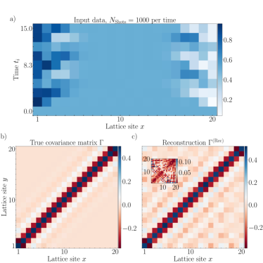
Figure 1: Tomographic reconstruction. a) Input data for the reconstruction based on out-of-equilibrium data of local particle numbers $N_{x}(t_{i})$ measured at $K=10$ equidistant times after the quench to nearest-neighbour hopping in the tilted lattice. We model statistical fluctuations by sampling occupation numbers $\mathcal{N}_{\text{Shots}}=10^{3}$ times for each $t_{i}$ and estimating $N_{x}(t_{i})$ via the empirical mean. b) The input data have been obtained by evolving a thermal covariance of $\hat{H}_{\text{NN}}$ with inverse temperature $\beta=3$ such that there are relatively large currents to be recovered. c) Results of the reconstruction $\Gamma^{(\rm Rec)}$. The extent of deviations shown in the inset is $\max|\Gamma_{x,y}-\Gamma^{(\rm Rec)}_{x,y}|\approx 0.1$ and is explained by the fact that among the data some $N_{x}(t_{i})$ can fluctuate statistical by two or three standard deviations.

The reconstruction is based on an algorithm that in a nut-shell takes a guess for the covariance matrix $\Gamma^{\prime}$, evolves forward to the times $t_{i}$ where the particle number data has been measured and checks whether the extrapolated distribution of the particles $N_{x}(t_{i};\Gamma^{\prime})=\Gamma^{\prime}_{x,x}(t_{i})$ reproduces the data $N_{x}(t_{i};\Gamma^{\prime})\approx N_{x}(t_{i})$. In the next step, an improved guess $\Gamma^{\prime\prime}$ is obtained, such that the new observables $N_{x}(t_{i};\Gamma^{\prime\prime})$ are closer to the data

$$|N_{x}(t_{i};\Gamma^{\prime\prime})-N_{x}(t_{i})|\leq|N_{x}(t_{i};\Gamma^{\prime})-N_{x}(t_{i})|\ .$$ (13)

By iterating this, the algorithm solves the following optimization task. We collect all measured data into a vector $b$, and define a linear map $\mathcal{A}$ which from an input covariance matrix $\Gamma^{\prime}$ produces the respective occupation numbers $N_{x}(t_{i};\Gamma^{\prime})$ in the same ordering as in $b$. The reconstruction $\Gamma^{\text{(Rec)}}$ is the optimal solution to the optimization problem

$$\min_{0\preceq\Gamma^{\prime}\preceq\mathds{1}}\|\mathcal{A}(\Gamma^{\prime})-b\|_{2}\ .$$ (14)

The cost function is the 2-norm so we need to perform a least-square recovery problem with a positivity constraint Diamond and Boyd (2016). Convexity of the problem guarantees an efficient convergence to a globally optimal solution with a polynomial runtime in the system size $L$ and desired accuracy $\epsilon>0$ Diamond and Boyd (2016) and in practice takes a few seconds for $L\approx 40$.

To exemplify the functioning of the method we consider thermal states $\hat{\varrho}_{\beta}=e^{-\beta\hat{H}_{\text{NN}}}/Z_{\beta}$, where $Z_{\beta}$ is the partition function, $\beta>0$ is the inverse temperature and $\Gamma^{(\beta)}$ is the corresponding covariance matrix. The results of the numerical reconstruction Gluza are presented in Fig. 1. The particle number measurement need not be perfect and Fig. 1 discusses reconstructions that include statistical noise from necessarily finite numbers of measurements.

In step (a), additional assumptions can be included such as translation invariance in the initial state or a finite correlation length. The quench is motivated by existing control functionalities, see, e.g., Ref. Preiss et al. (2015) for an experimental study showcasing a superb degree of coherence in the system when tilting the optical lattice. We remark that other quenches that lead to non-trivial dynamics (the covariance matrix is not a steady state of the quench Hamiltonian) can be considered. The reconstruction code Gluza does not depend on the quench Hamiltonian being nearest-neighbour, or whether there is a trap present so other variants are possible, see the appendix. If the couplings $h$ are real, then the tomography reconstructs only the real part of the currents. This is enough for thermal states of quadratic Hamiltonians with no magnetic fields, see the appendix for reconstructions in their presence. Finally, note that similar ideas have successfully been applied in an atom chip experiment for a continuum system Gluza et al. (2020) where some unknown stray interactions have been present Rauer et al. (2018) but have been negligible in short time windows.

Quantum simulation studies of low-temperature systems in presence of Hubbard interactions with strength $U$ are of particular interest. Our method can be used to measure the second moments of interacting states by switching-off $U\mapsto 0$ as fast as possible, e.g., by choosing narrow Feshbach resonances, see the appendix for comparisons of ramps of varying duration compared to the tunnelling time. Crucially though, it follows directly from the Lieb-Robinson bound Lieb and Robinson (1972) that even if the quench has a finite duration then only the local correlations will be affected but, e.g., the presence of long-range order can be reliably inferred. If the quench has a negligible duration compared to the relevant time-scales in the system then even local correlations will be faithfully reconstructed implying the possibility of measuring also the kinetic energy in addition to the Hubbard interaction term that can be measured with the atom microscope. Our method does not assume translation invariance or thermality of the unknown state which are the corner stones but also limitations of existing methods Hartke et al. (2020); Nichols et al. (2019); Brown et al. (2019); Takasu et al. (2020); Nakamura et al. (2019); Cocchi et al. (2017); Chan et al. (2020); Guardado-Sanchez et al. (2020) and hence can pave the way towards reading out the results of variational quantum simulations Kokail et al. (2019) in optical lattices for systems with a complicated connectivity graph.

Quantitatively estimating fermionic mode entanglement. Let us now show how to analyze the second moments $\Gamma$ of a possibly interacting or non-equilibrium state to lower bound the so-called entanglement cost Bennett et al. (1996); Horodecki et al. (2009). This statement is particularly appealing as it goes beyond merely showing that there is entanglement present, but provides an answer to the question of “how much” entanglement is there in the system Eisert et al. (2007); Audenaert and Plenio (2006); Guehne et al. (2007); Cramer et al. (2013). The entanglement cost $E_{C}$ quantifies mixed-state entanglement Bennett et al. (1996); Horodecki et al. (2009) as it is the asymptotic rate at which maximally entangled pairs must be used for the creation of a given state $\hat{\varrho}$ using local operations with classical communication (LOCC). $E_{C}$ is broadly studied in quantum information theory but is not easy to access in practice and therefore, especially in context of experiments, lower bounds by means of practically measurable quantities are needed.

We consider $\hat{\varrho}$ to describe a bipartite system $A\cup B$, e.g., some number of sites in an optical lattice, and will explain how to lower bound $E_{C}(\hat{\varrho})$. Firstly, if the asymptotically optimal creation of the state $\hat{\varrho}$ via LOCC necessitates maximally entangled pairs at rate $E_{C}(\hat{\varrho})$ then it could be that even more entangled pairs are needed for a system consisting of fermionic particles. Indeed, any physical operation in this case is subject to the fermionic parity and total number super-selection rules (SSR) Earman (2008); Wick et al. (1952) which further restrict LOCC. However, in Ref. Schuch et al. (2004a), it has been shown that the asymptotic rates do not change, i.e., $E_{C}^{\rm SSR}(\hat{\varrho})=E_{C}(\hat{\varrho})$ (see the appendix). Secondly, we use that entanglement cost is lower bounded by distillable entanglement $E_{D}$ Bennett et al. (1996); Horodecki et al. (2009)

$$E_{C}(\hat{\varrho})\geq E_{D}(\hat{\varrho})\ .$$ (15)

In fact, in our discussion, we can equally well also refer to the distillable entanglement. Thirdly, the distillable entanglement is lower bounded by virtue of the hashing bound Devetak and Winter (2005)

$$E_{D}(\hat{\varrho})\geq S(\hat{\varrho}_{A})-S(\hat{\varrho}),$$ (16)

where for any state $\hat{\sigma}$ the von Neumann entropy is $S(\hat{\sigma})=-\operatorname{tr}[\hat{\sigma}\log_{2}(\hat{\sigma})]$ and the subscript in $\hat{\varrho}_{A}$ indicates the the reduction to subsystem $A$. Finally, the right hand side can be lower bounded by the same expression but now in terms of Gaussian entropies. Specifically, let us denote by $S^{(\Gamma)}=S(\hat{\varrho}_{\Gamma})$ to be the von Neumann entropy of a fermionic Gaussian state $\hat{\varrho}_{\Gamma}$ with the same second moments $\Gamma$ as $\hat{\varrho}$. As shown in Refs. Pastawski et al. (2017); Eisert and Wolf (2007) we have

$$S(\hat{\varrho}_{A})-S(\hat{\varrho})\geq S^{(\Gamma_{A})}-S^{(\Gamma)}:=E_{G}(\Gamma)\ .$$ (17)

The Gaussian entropy $S^{(\Gamma)}$ can be easily computed from the recovered covariance matrix $\Gamma^{\text{(Rec)}}$, see the appendix for details. Summarizing, for any bipartite state $\hat{\varrho}$ whose second moments $\Gamma$ one can measure using our method we have found a lower bound to the entanglement cost $E_{G}(\Gamma)\leq E_{C}(\hat{\varrho})$.

Entanglement cost at finite temperatures. In what follows we discuss the application of the witness to again assess thermal states of $\hat{H}_{\text{NN}}$. As detailed in the appendix without increasing $E_{C}$ we can perform a local unitary Bogoliubov transformation in subsystems $A$ and $B$ individually. In Fig. 2a) we show the covariance matrix for $\beta=3$ after such a local transformation showing that essentially two modes are non-trivially correlated. In Fig. 2b) we depict the entanglement cost lower bound $E_{G}(\beta){{\color[rgb]{0,0,0}:=}}E_{G}(\Gamma^{(\beta)})$ as a function of inverse temperature. We select either one or two modes in each subsystem and find a non-trivial lower bound $E_{G}(\beta)>0$ for sufficiently low temperatures. Choosing one mode gives a non-trivial lower bound for higher temperatures than for two modes because the total entropy in the latter case tends to be larger at high temperature. In contrast, at extremely low temperatures, the one mode lower bound saturates at its maximum value $E_{G}^{(1+1)}(\beta)\leq 1$ while the two mode witness indicates that the entanglement cost of preparing $\hat{\varrho}_{\beta}$ is asymptotically larger than that of one maximally entangled pair. Going beyond the Gaussian case, note that the second moments of low-temperature states will vary continuously with the strength of the many-body interaction Kraus and Cirac (2010). Thus we can be confident that a non-trivial $E_{C}$ lower bound will be obtained for sufficiently weak interactions and low temperatures. Such states, e.g., in two spacial dimensions become difficult to treat numerically in practice, however, our reconstruction and entanglement quantification methods remain applicable for quantum simulations.

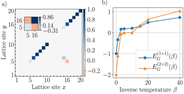
Figure 2: Entanglement cost at finite temperature. a) The covariance matrix $\Gamma^{(D)}=U_{D}\Gamma^{(\beta)}U_{D}^{\dagger}$ for the inverse temperature $\beta=3$ after a suitable local transformation $U_{D}=U_{A}\oplus U_{B}$ preserving the entanglement. The inset shows the sub-matrix of the covariance matrix reflecting one mode in subsystem $A$ and one in $B$. b) This figure shows how the lower bound for the entanglement depends on whether it is applied on one or two modes in systems $A$ and $B$ each. Selecting merely one mode each provides a positive entanglement cost for relatively large temperatures ($E_{G}^{(1+1)}$), while two modes are better suited to detect entanglement at low temperatures ($E_{G}^{(2+2)}(\beta)$).

Outlook. In this work, we have shown how to recover the full covariance matrix of quantum states in optical lattices by unifying atom microscope measurements with suitable quenches and performing efficient reconstructions using semi-definite programming. The method introduced here is reliable and versatile as it does not depend on the geometry of the quench: Other ways of inducing visible particle number dynamics specific to a given setup can also be considered and some other ideas are discussed in the appendix. The prospect of advancing our data analysis by making use of recent theoretical ideas such as shadow estimation Huang et al. (2020) or random operations that can be efficiently classically back-tracked Ohliger et al. (2013); Brydges et al. (2019) should also be noted. Building on the accessibility of full covariance matrices, including coherent currents, we have exploited an entropic witness that allows to lower bound the entanglement cost and the distillable entanglement. This is a quantitative measure of entanglement implying a substantially stronger statement than merely showing its presence. We have shown that our witness can give non-trivial values at finite temperatures. This will remain true also for weak interactions as second moments should vary continuously in the strength of interactions. We hence, have established a method to recover and quantify quantum correlations in optical lattice quantum simulations which is applicable even in regimes where numerical calculations cease being practical.

Acknowledgements. We thank M. Greiner, C. Gross, P. Preiss and R. Sweke for stimulating discussions. This work has been supported by the ERC (TAQ), the DFG (CRC 183, FOR 2724, EI 519/7-1), the BMBF (DAQC), and the Templeton Foundation. This work has also received funding from the European Union’s Horizon2020 research and innovation programme under grant agreement No. 817482 (PASQuanS).

Appendix

This appendix provides substantial detail of the arguments of the main text, and corroborates the conclusions drawn there by further analysis. It is organized as follows. In Section A, we provide additional statistical and systematic analysis if the “tilting” protocol presented in the main text. We also show the results of recoveries based on two other examples of initial conditions, this time non-translation invariant. In Section B, we discuss an additional protocol based on doubling of the optical lattice. In Section C, we provide more simulations testing a line of ideas for other protocols. In Section D, we introduce some ideas for benchmarking in the experiment the doubling protocol, with the aim to experimentally infer how well it works. In Section E, we show additional simulations for the analysis of finite durations of switching off the interactions in a Hubbard chain. Finally, in Section F, we go into great detail presenting further material on the entropic entanglement witness presented in the main text and its numerical evaluation.

Appendix A Additional reconstructions

A.1 Analysis of performance for finite sample sizes and single-shot statistics

In this section, we provide a description of the procedure we have used to simulate the single-shot outcomes, beyond the mere use of expectation values. This is motivated by experiments employing the atom microscope, e.g., the expectation value $\langle\hat{N}_{x}(t)\rangle\approx 0.5$ has to be estimated by averaging a series of individual outcomes which are either $0$ (particle is absent) and $1$ (particle is present). We next describe how to simulate such single-shot measurements.

At a fixed time $t>0$, the occupation number operators commute $[\hat{N}_{x}(t),\hat{N}_{y}(t)]=0$, a feature that implies that the measurement of one does not influence the measurement outcome of the other. For this reason, the single-shot outcomes of the measurement of each $\hat{N}_{x}(t)$ can be “parallelized” and obtained from the reduced density matrix on the mode located at $x$. This is a $2\times 2$ matrix which can be taken to be

$$\hat{\varrho}_{x}(t)=\text{diag}(p,q):=\begin{pmatrix}\langle\hat{N}_{x}(t)\rangle&0\\ 0&1-\langle\hat{N}_{x}(t)\rangle\end{pmatrix}\ .$$ (18)

Thus, to simulate the outcomes of atom number measurements at a position $x$ and time $t_{i}$ in the optical lattice in $\mathcal{N}_{\text{sample}}(t_{i})$ experimental runs we can simply sample $\mathcal{N}_{\text{sample}}(t_{i})$ times from the Bernoulli distribution with

$$p=\langle\hat{N}_{x}(t_{i})\rangle.$$ (19)

Performing this step for all lattice sites, we obtain a simulation of the random outcomes of the measurements in the entire system. Finally, this should be repeated for each measurement time $t_{i}$ to simulate the what would be the outcome of an experiment. In order to assess the performance of the tomographic recovery procedure, we iterate over all times $t_{i}$ and positions $x$ and compute the empirical estimate of the mean particle number

$$\langle\hat{N}_{x}(t_{i})\rangle\approx\frac{1}{\mathcal{N}_{\text{sample}}(t_{i})}\sum_{j=1}^{\mathcal{N}_{\text{sample}}(t_{i})}N_{x}^{(j)}(t_{i})$$ (20)

where $N_{x}^{(j)}(t_{i})\in\{0,1\}$ is the $j$-th outcome of either having or not having the particle at position $x$ and time $t_{i}$. The estimated atom numbers $N_{x}(t_{i})$ are then taken as the input to the reconstruction.

We then repeat this approach a sufficiently large number of times and each time we run the tomography. The finite number of single-shot outcomes leads to statistical errors in the estimation of the genuine expectation values $\langle\hat{N}_{x}(t_{i})\rangle$ which then propagates into the fidelity of the reconstructed matrix. What we find is that generically the noise leads to the introduction of stray off-diagonal correlations as shown in the main text, while the overall correlation pattern for entries of the covariance matrix of substantial magnitude are not overturned by noise. For example, for $\mathcal{N}_{\text{Total}}=10.000$ total state preparations distributed over $\mathcal{N}_{\text{Times}}=10$ measurement times we find that the relevant currents in the thermal covariance matrix of the nearest-neighbour Hamiltonian can be clearly discerned with good signal to noise ratio. These parameters have been used in the reconstruction result shown in the main text based on a random sample of occupation numbers. In Fig. 3, we show the cumulative results after running the tomography 500 times to assess the typical and worst-case results of the procedure. We show that repeating the procedure many times it is possible that a rare event can happen in that a matrix element of the reconstructed covariance matrix will largely deviate from the true value. However, such rare events are just a result of random sampling repeated many times (unlikely but possible events will happen eventually if one tries sufficiently often) and most results concentrate around the median or mean taken over the maximal deviations.

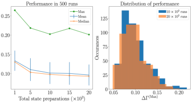
Figure 3: Dependence of the reconstruction fidelity on the sampled atom occupation numbers. For each run $j=1,\ldots,500$ of the tomography we consider the maximal deviation $\Delta\Gamma^{(j)}=\max|\Gamma_{x,y}-\Gamma^{(\rm{Rec},j)}_{x,y}|$ of the reconstructed covariance matrix $\Gamma^{(\rm{Rec},j)}$ from the true covariance matrix $\Gamma$. In panel a), we show the mean ($\mathbb{E}_{j}[\Delta\Gamma^{(j)}]$) and median ($\text{Median}[\Delta\Gamma^{(j)}]$) of the maximal deviation in dependence of the total number of experimental runs. The presence of large maximal deviation ($\max[\Delta\Gamma^{(j)}]$) can be explained by the many repetitions of the reconstruction procedure and as is shown in the histograms in panel b) most results concentrate around the mean and median while the large deviations happen only rarely.

A.2 Dependence on the number of measurement times

Another aspect to consider, one we dedicate this section to, is how to best choose the discrete and equally spaced measurement times. There are two parameters to consider when working with equidistant times. These are on the one hand the total evolution time $T$ and on the other hand the number of measurement times $K$. The quench evolutions that we consider in this work feature an effective causal cone confined by the Lieb-Robinson bound Hastings and Koma (2006), which in turn is implied by the locality of the Hamiltonian

$$|G_{x,y}(t)|\leq C_{\text{LR}}e^{-|x-y|+v_{\text{LR}}t}.$$ (21)

Here, we have denoted by $v_{\text{LR}}>0$ the Lieb-Robinson velocity. For this reason one can develop an intuition that the total evolution time should be sufficiently long such that the particle number dynamics in the relation discussed in the main text

$$N_{x}(t) =\sum_{y,y^{\prime}=1}^{L}G_{x,y}(t)G_{x,y^{\prime}}^{*}(t)\Gamma_{y,y^{\prime}}(0)$$ (22)

$$\approx\sum_{|y-x|\leq 2v_{\text{LR}}t}^{L}\sum_{|y^{\prime}-x|\leq 2v_{\text{LR}}t}^{L}G_{x,y}(t)G_{x,y^{\prime}}^{*}(t)\Gamma_{y,y^{\prime}}(0)\$$ (23)

has a chance to be large. Here, the approximation made has neglected the exponentially suppressed terms in the radius of an enlarged Lieb-Robinson cone $d_{\text{LR cone}}(t)=2v_{\text{LR}}t$. For this reason, it seems that the evolution time $T>0$ should be large enough such that the influence of the relevant currents is not exponentially suppressed. Even for ideal data, in such a case a reconstruction should be possible in principle, but issues of numerical stability can come into play and either way, in the presence of statistical noise one wants to have as visible dynamics as possible. Fig. 4 shows the result for $T=15$ and $L=10$. We have performed a tomographic recovery based on measurements taken at varying interval spacing with the intention to see how the time spacing of the measurements influences the quality of the reconstruction. As we see, quite quickly the reconstruction becomes accurate and the relevant currents narrow down around their true values.

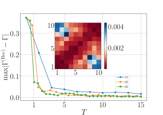
Figure 4: Dependence of the reconstruction fidelity on the number of measurement times. For $L=10$ and $T=15$ we consider the time spacing $\Delta T:=T/K=2/3,1,3/2$ ($K=10,20,30$, respectively). For each $\Delta$ we perform a tomographic recovery without the presence of statistical noise for varying number of consecutive points with the respective bullet corresponding to the end of the interval. We see a rapid decay of the reconstruction residue, reflecting the fact that the bulk features of the correlations can be inferred with relatively little input. The slight non-monotonicity in the $K=30$ curve can be explained that for tomographically incomplete inputs there is a number of covariance matrices consistent with the input data and the slightly increased deviation when providing more input can be an unlucky nudge in the wrong direction in this set of covariance matrices which are equivalent on the level of $N_{x}(t)$. Such behaviour becomes even less pronounced for sufficiently large numbers of inputs. The inset shows the full reconstruction residue matrix with elements $|\Gamma^{(\rm Rec)}_{x,y}-\Gamma_{x,y}|$ for $K=30$ input times and indicates that the source of the deviations is the difficulty in constraining the far-away correlations based on the input dynamics. When appropriate, suppressing such artefacts can be done by making use of prior knowledge and penalizing additionally correlations between far-way points.

A.3 Reconstruction of a disordered initial state

In the example discussed in this section, we consider a thermal state of the Anderson insulator model

$$\hat{H}_{\text{Anderson}}=\hat{H}_{\text{NN}}+\sum_{x=1}^{L}\nu_{x}\hat{N}_{x}$$ (24)

where $\nu_{x}\in[-0.3,0.3]$ has been chosen independently and identically at random for each $x$. Using such a Hamiltonian, we construct a thermal ensemble

$$\hat{\varrho}_{\text{Anderson}}(\beta)=e^{-\beta\hat{H}_{\text{Anderson}}}/Z_{\beta},$$ (25)

where $Z_{\beta}>0$ again denotes the partition function. We take the inverse temperature to be $\beta=3$ and denote by $\Gamma^{(\rm Anderson)}$ the covariance matrix of $\hat{\varrho}_{\text{Anderson}}(\beta)$.

Fig. 5 shows a reconstruction for one realization of such a random initial condition. This is an instructive initial condition because we see that the reconstruction correctly detects the regions where the particles are delocalized within the small regions allowed by the typical Anderson localization length. In those restricted regions, the particles roam freely as evidenced by the off-diagonal correlations in the initial state but also in the reconstructed state, despite the random noise coming from taking into account a finite number of state preparations.

This demonstrates that our tomographic reconstruction method can detect the coherences in random ensembles where there is essentially no prior information to the character of the correlations. To the best of our knowledge, there is no other method delivering these important observables as very many methods make simplifying assumptions such as translation invariance or thermal equilibrium of a known model. It is beyond the scope of this work to illustrate the versatility of the method in all of its ramifications, but it is worth pointing out that one can equally well perform such reconstruction for the second moments of interacting states and thus study many-body localization. In this context, the covariance matrix has been shown to reveal insights about this genuinely non-Gaussian phenomenon Bera et al. (2015).

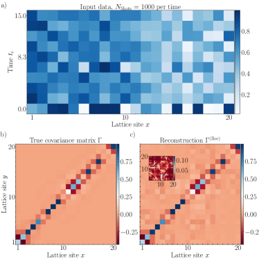
Figure 5: Reconstruction of a disordered initial condition. After sampling the on-site disorder $\nu_{x}$ we have computed the thermal covariance matrix of the Anderson model with $\beta=3$. The reconstructed covariance matrix (panel c) closely matches the true covariance matrix (panel b) with the coherences being accurately reproduced with a clear signal to noise ratio.

A.4 The role of compressibility when reconstructing based on gradients of the chemical potential

In this section, we comment on a curious feature of the particle number dynamics that can be seen in the figure shown in the main text. This is the feature that the bulk of the system is not influenced by the quench adding a gradient of the chemical potential, but rather only the edges are affected by this. One could think that the lack of visible atom number dynamics would hint at an absence of currents. Indeed, if we consider any internal quench in a non-interacting and isolated system, then states entirely lacking currents would feature any visible dynamics. This can be seen by translating the above statement into some Greens function $t\mapsto G_{\text{Quench}}(t)$, the unitary single-particle Greens function. Homogenous states lacking currents feature covariance matrices which are multiples of the identity $\Gamma^{(\rm NoCurrents)}=\alpha\mathds{1}$ and for any $0<\lambda<1$ we have that there will be no dynamics

$$\Gamma^{(\rm NoCurrents)}(t) = G_{\text{Quench}}(t)\Gamma^{(\rm NoCurrents)}(0)G_{\text{Quench}}(t)^{\dagger}$$ (26)

$$= \Gamma^{(\rm NoCurrents)}(0)G_{\text{Quench}}(t)G_{\text{Quench}}(t)^{\dagger}$$

$$=: \Gamma^{(\rm NoCurrents)}(0).$$

We are then lead to the following conclusions: Covariance matrices invariant under all non-interacting quenches in an isolated system are those reflecting product states (or infinite temperature states). In particular, these states are incompressible, and gradients of the chemical potential do not modify their density distribution.

In the main text, we have seen that the bulk of the system remains homogenous, but as it turns out, it reveals the information that the system is homogenous everywhere and has currents in the bulk matching the currents present at the edges. This can be seen in Fig. 6 where we consider a quench into the nearest-neighbour Hamiltonian together with a chemical potential gradient (exactly as in the main text), but now for a fiducial state that can be thought of as a composition of a chain in the superfluid state, then a very hot chunk in the infinite temperature state and then again a superfluid. As shown in the figure, the system responds with markedly different atom number dynamics than a homogeneous state. We conclude from this that the atom number dynamics influenced by the gradients of the chemical potential is sensitive to the presence or absence of initial correlations. The depletions and increases of the density of the gas over time we can interpret as “breathing” of the gas related to spatially varying compressibility. By the equation of state compressibility is related to the temperature.

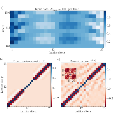
Figure 6: Reconstruction of an inhomogeneous state. We exemplify the reconstruction of an initial condition which includes a block with no correlations. a) The presence of this block visibly modifies the atom number dynamics. b) The initial covariance matrix is faithfully reconstructed (c) even despite the noise (see inset for the difference).

Appendix B Reconstructions using a quench into a sub-lattice

The full recovery of the covariance matrix $\Gamma$ is actually possible by means of suitable choices of the quench involved in the protocol. In this section, we provide some ideas for a more sophisticated protocol which involves a step of quenching into a sub-lattice. To state the protocol, we follow along the lines presented in the main text. The first step is again preparing the state of interest:

$$\text{(a) Prepare a fermionic state }\hat{\varrho}.$$ (27)

We then split the quench into two steps. As the second step, the task is:

$$\text{(b') Double-up the lattice locally }\hat{f}_{x}\mapsto\hat{f}_{2x-1}\ .$$ (28)

In Fig. 7b), we illustrate this by assuming that the system has initially been in a thermal state of Eq. (5) with a translationally invariant covariance matrix and a finite correlation length. We assume the doubling is fast and the in-between sites are still unoccupied while the correlations between the original sites have remained unchanged which gives rise to a distinct checker-board correlation pattern. The fast doubling is in many experimental situations actually a highly plausible assumption and perfectly feasible.

Next, we shall use coherent evolution under Eq. (5) to mix information about the coherent current into the particle number occupation operators:

$$\text{(b'') Quench to a free Hamiltonian }\hat{H}_{\text{NN}}.$$ (29)

In Fig. 7a), we depict the resulting atom number dynamics. In the last step, again the local atom numbers should be measured

$$\text{(c) Measure }N_{x}(t):=\langle\hat{N}_{x}\rangle_{\hat{\varrho}(t)}\ .$$ (30)

As shown in Fig. 7c), an accurate reconstruction can be achieved from this protocol even in the presence of finitely many state preparations.

Figure 7: Tomographic reconstruction. a) Input data for the reconstruction based on out-of-equilibrium data of local particle numbers $N_{x}(t_{i})$ estimated from $\mathcal{N}_{\text{Shots}}=10^{3}$ shots per measurement time $t_{i}$ with in total $K=10$ equidistant times after the quench to nearest-neighbour hopping in the superlattice. b) The input data have been obtained by evolving a thermal covariance with inverse temperature $\beta=3$. We have chosen a temperature so that there are relatively large currents to be recovered. The covariance matrix $\Gamma$ is shown after step (b’) after the sub-lattice has been created. Note that besides the new checker-board pattern, the correlations between sites are assumed to be exactly preserved. c) Results of the reconstruction $\Gamma^{(\rm Rec)}$ and the extent of the deviations shown in the inset is $\max|\Gamma_{x,y}-\Gamma^{(\rm Rec)}_{x,y}|\approx 0.05$.

B.1 Ramping up instead of quenching into doubled lattice

The protocol involving the step (b’) where the lattice is doubled is more complex, in that it involves an additional step. This step is what we assess in this section with respect to its feasibility. From the perspective of current experimental implementations, performing this step seems rather straightforward: The periodicity of the lattice is controlled by the trapping lasers which create the optical lattice and can be tuned rather fast. In what follows, we model the systematic imperfection stemming from such a doubling ramp as follows. For this purpose, we introduce a new fermionic mode in-between each consecutive pair of modes in the initial lattice. We initialize that mode in a vacuum state. This, in particular, implies that there is no correlations to any other site and so for simulating a finite duration of the doubling the initial covariance matrix will be

$$\Gamma^{\rm(b^{\prime})}=\Gamma^{(\text{Ini})}\otimes\begin{pmatrix}0&0\\ 0&1\end{pmatrix}.$$ (31)

Here, we involve a method using the Kronecker product to concisely write the effect of the doubling in (b’) and $\Gamma^{\rm(b^{\prime})}$ if the doubling was perfect this would be the perfect state preparation. We then model the gradual appearance of the in-between sites over time $t$ by performing an interpolation of the Hamiltonians

$$\hat{H}_{\text{Doubling}}(t)=(1-t/T_{\text{Doubling}})\hat{H}_{\text{NNN}}+t/T_{\text{Doubling}})\hat{H}_{\text{NN}}.$$ (32)

Here, $T_{\text{Doubling}}>0$ parametrizes the duration of the doubling and $\hat{H}_{\text{NNN}}$ is the next-next-nearest neighbour hopping Hamiltonian which arises from the fact that the next-nearest neighbour sub-lattices were initially the system of interest and the auxiliary unoccupied sites. We then perform an evolution to time of $\Gamma^{\rm(b^{\prime})}$ under the time-dependent Hamiltonian $\hat{H}_{\text{Doubling}}(t)$ using a standard Trotterization scheme and obtain the covariance matrix $\Gamma^{\rm(b^{\prime})}(T_{\text{Doubling}})$ which encodes the imperfections stemming from the finite duration of the doubling. This systematic deformation $\Gamma^{\rm(b^{\prime})}\mapsto\Gamma^{\rm(b^{\prime})}(T_{\text{Doubling}})$ would not be detected by the tomographic reconstruction as it would assume an instantaneous quench (though if the ramp is known it can be included in the parametrization of the reconstruction).

In Fig. 8, we display the results of an analysis of the fidelity of the state preparation involved in step (b’) by performing an additional numerical analysis. Qualitatively, one observes that the checker-board pattern melts rapidly whenever $T_{\text{Doubling}}\approx 1$ is of the order of the tunnelling time. The dynamics occurs again locally, so most of the dynamics is concentrated around the diagonal. We do not go into the details of this evolution but rather show global figures of merit: We consider the matrix of the absolute values of differences between the entries of the ramped and ideal covariance matrices $|\Gamma^{\rm(b^{\prime})}-\Gamma^{\rm(b^{\prime})}(T_{\text{Doubling}})|$ and convert them into a scalar by taking a maximum, mean or a median over all entries. We find that if the doubling occurs at a small fraction of the tunnelling time $T_{\text{Doubling}}\ll 1$, then the ramp will not make a difference and will not substantially impact the state that will be reconstructed.

This modelling does not account for other possible imperfections involved in the doubling of the lattice. In particular, it seems that ensuring that the atoms remain in the lowest band of the lattice at each time of the state preparation (b’) is the most immediate concern. Not accounting for this (or possibly not mitigating for it by optimal control) would possibly result in an instance of a “heating” in the experiment, at least unless precise band mapping would uncover the band excitations. Having said that, given that the atoms at each lattice site do not have a large extension within the local well the fraction of band excitations should be small. Qualitatively, it should be related to the spatial “squeezing” of the local atom wave-function which is needed to restrain the particles into wells of a reduced size. Further analysis is beyond the scope of this appendix, but in principle one could once more extend our modelling to couple the system of primary interest to auxiliary unoccupied “sites” of the higher excitation bands. The coupling constants for this would however depend on the optimality of the time-dependent ramp involved which would depend on whether there is a global harmonic trap present or it has been flattened in the region of interest by additional light fields using a digital-mirror device.

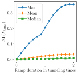
Figure 8: Effect of the final ramp for the doubled lattice on initial correlations. If one assumes a finite time $T_{\text{Ramp}}$ for the duration of the transition between the initial and the doubled-up lattice then the initial correlations will be deformed. The extent of deviations is $\Delta\Gamma=\max|\Gamma_{x,y}-\Gamma^{(\rm Rec)}_{x,y}|$ and is seen to be negligible for small $T_{\text{Ramp}}\ll 1$ (much less than a tunnelling time) and $T_{\text{Ramp}}$ not negligible compared to the tunnelling time.

Appendix C Choosing an appropriate quench Hamiltonian

In this section, we come back to some relevant observations regarding the choice of the quench Hamiltonian $h_{\text{Quench}}$. This material is intended to provide further insights into how one can see that a quench does not provide enough atom number dynamics to facilitate a reconstruction for researchers interested in implementing the reconstruction based on the response of the gas to other protocols than the tilting or doubling of the lattice as presented above. Our first example is motivated by notions of time of flight measurements: What happens, after all, if we just simply let the gas expand? Fig. 9 shows that such an approach is not sufficient because in the optical lattice the gas expands ballistically outwards and the particles moving at the front do not mix with the ones propagating behind them. We see that according with this intuition the reconstruction fails to detect currents for the thermal initial condition shown in the main text. That said, if this approach does not quite work do to a lack of mixing, then how about mixing with an auxiliary system? After all, we are interested in coherent tunnelling events which could in some formalisms be related to non-zero derivatives of an appropriately defined “phase” and hence interference could possibly be used to uncover the currents. Fig. 10 shows that choosing an incoherent charge-density wave as the auxiliary system does not actually lead to a correct reconstruction. A possible explanation is that the tunnelling currents should be seen as “coherences” and the mixing to the incoherent system is insensitive to these correlations. Finally, as we show in Fig. 11, an expansion constrained by a hard-wall implemented by a sudden increase of the chemical potential allows for reconstructions of the coherent tunnelling currents. We have chosen a quench Hamiltonian where the gas can expand through three sites to its left and right via nearest-neighbour hopping but then suddenly the hopping is obstructed by a sudden jump in the chemical potential

$$\mu_{x}=\begin{cases}100,&x<-3\\ 0,&-3\leq x\leq L+3\\ 100,&x>L+3.\end{cases}$$ (33)

Summarizing, caution is necessary when choosing the precise form of the quench Hamiltonian. In particular, quenches inducing “coherent” mixing within the system turn out to be necessary to uncover the “coherences”, i.e., the tunnelling currents. This intuition seems to be well grounded in the examples provided above. Having said that, we would like to point out that a full characterization of the tomographic resourcefulness of a given quench protocol occurs to be an interesting open problem which seems to be challenged by the wealth of possible quench ideas that one can consider as exemplified above.

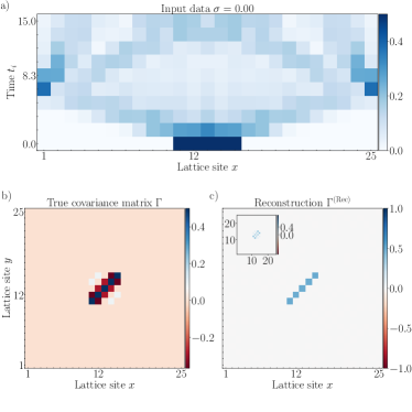
Figure 9: Ballistic expansion. Allowing the gas to suddenly expand is not an appropriate choice for $h_{\text{Quench}}$ because the atoms just move outwards quickly and do not mix together in the process (panel a)). As in the main text, we use the thermal initial condition of the nearest neighbour hopping Hamiltonian (panel b) as the initial condition and the reconstruction does not uncover the currents in the state. This indicates that in the ballistic expansion the atom occupation numbers are not influenced by the presence or absence of tunnelling currents.

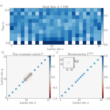
Figure 10: Mixing with a charge-density wave. We consider the possibility of measuring the currents by interfering a system with atoms that were held at fixed positions at its sides. As before, we make use of a thermal initial condition of the nearest neighbour hopping Hamiltonian (panel b) as the initial condition. Once more, for this candidate choice of tomographic quench the reconstruction does not uncover the currents in the state. This indicates that in the mixing with charge-density waves on the sides is incoherent in the sense that the atom number dynamics is insensitive to the “coherence”, i.e., the tunnelling currents.

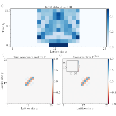
Figure 11: Expansion into a hard-wall trap. We consider once again a ballistic expansion, but now constrained by hard walls on both sides of the system. As in the previous examples we use the thermal initial condition of the nearest neighbour hopping Hamiltonian (panel b) as the initial condition. In this case, we find that the reconstruction has successfully uncovered the currents in the state implying that in the mixing induced by the reflections from the walls is sensitive to the currents. This protocol can be viewed as an abstraction of the quench shown in the main text involving the tilting of the lattice: In both cases the atoms are moving on top of each other with reflections occurring during the dynamics.

C.1 Symmetries of the Hamiltonian

Various symmetries of the Hamiltonian may lead to some aspects of the state to remain hidden in the tomographic recovery procedure, or more precisely some correlation functions may be unconstrained by the observed particle number dynamics. Such symmetries are discussed here. Some simple examples are the following.

(i) Hopping Hamiltonians mix correlations within the tunnelling correlation sector only. Therefore pairing correlations such as $\langle\hat{f}_{x}\hat{f}_{y}\rangle+\text{h.c.}$ can be arbitrary and their presence or absence does not modify the input to the tomographic recovery procedure.

(ii) If both the initial state and the quench Hamiltonian are translation invariant then even if there are non-trivial currents in the covariance matrix, the particle number dynamics remains unchanged. This can be seen by observing that both $h$ and $\Gamma(0)$ can be simultaneously diagonalized by a Fourier transform and so their commutator vanishes at all times. This implies that $N_{x}(t)=\Gamma_{x,x}(t)=\Gamma_{x,x}(0)=N_{x}(0)$ and the currents are unconstrained. We resolved this issue by doubling up the lattice which implies that every other site is unoccupied and necessarily the state is not translation invariant.

The case when the couplings $h$ are real is related to the absence of magnetic fields. We will now show that if one quenches to a Hamiltonian with such couplings, then only the real part of the currents can be reconstructed. That is to say, let the state have some second moments $\Gamma=\Gamma^{(\rm Re)}+i\Gamma^{(\rm Im)}$ with $\Gamma^{(\rm Re)},\Gamma^{(\rm Im)}$ being the real and imaginary parts, respectively. Then the tomography performed using the measurement of particle numbers will not constrain the imaginary part covariance matrix.

Let us now demonstrate that the particle number dynamics does not depend on the initial imaginary part of the currents if the couplings $h$ are real. To see this, we note that $\Gamma^{(\rm Im)}=-{\Gamma^{(\rm Im)}}^{T}$ because $\Gamma=\Gamma^{\dagger}$. Secondly, we will use that $h=h^{T}$ implies $G(t)^{*}=G(-t)$ and $G(t)^{T}=G(t)$. The particle numbers at time $t$ are given by

$$N_{x}(t)=\Gamma_{xx}(t)=G(t)\Gamma^{\rm(Re)}G(t)^{\dagger}+iG(t)\Gamma^{\rm(Im)}G(t)^{\dagger}.$$ (34)

The first term related to the real part of the currents will in general influence the particle number dynamics. For the second term by transposing twice we see that

$$\Gamma^{\rm(Im)}(t): =G(t)\Gamma^{\rm(Im)}G(t)^{\dagger}$$ (35)

$$=\left(G(t)^{*}(\Gamma^{\rm(Im)})^{T}G(t)^{T}\right)^{T}$$

$$=-\left(G(-t)\Gamma^{\rm(Im)}G(-t)^{\dagger}\right)^{T}$$

$$=-\Gamma^{\rm(Im)}(-t)^{T}$$

and

$$\Gamma^{\rm(Im)}(t)^{*} =G(t)^{*}(\Gamma^{\rm(Im)})^{*}(G(t)^{\dagger})^{*}$$ (36)

$$=G(-t)\Gamma^{\rm(Im)}G(-t)^{\dagger}$$

$$=\Gamma^{\rm(Im)}(-t)\ .$$

The only way for the imaginary part of currents $\Gamma^{\rm(Im)}$ to contribute to particle number dynamics is via the diagonal matrix elements of its real part after the time evolution

$$\text{Re}[\Gamma^{\rm(Im)}(t)] =\frac{1}{2}(\Gamma^{\rm(Im)}(t)+\Gamma^{\rm(Im)}(t)^{*})$$ (37)

$$=\frac{1}{2}(\Gamma^{\rm(Im)}(t)-\Gamma^{\rm(Im)}(t)^{T})\ .$$

The last relation proves that the real part of $\Gamma^{\rm(Im)}(t)$ is an antisymmetric matrix. This implies that its diagonal matrix elements are vanishing and hence the imaginary part of the currents cannot be detected by the tomography after a quench to an evolution with real couplings so

$$\langle\hat{N}_{x}(t_{i})\rangle_{\hat{\varrho}_{\Gamma}}=\langle\hat{N}_{x}(t_{i})\rangle_{\hat{\varrho}_{{\rm Re}[\Gamma]}}\ .$$ (38)

The next section discusses this property further in relation to practical examples.

Appendix D Strategies for experimentally benchmarking the systematics of the sub-lattice quench on charge density waves

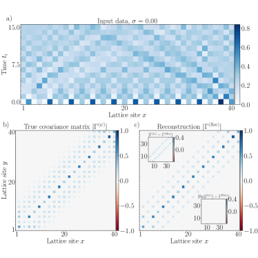
Figure 12: Reconstruction for quenched CDW. a) The particle number dynamics used in the quench. b) The same covariance matrix as above is to be reconstructed. c) The reconstruction has not detected the presence of a complex-valued current. The upper inset shows that certain tunnelling correlation are missing, these precisely the imaginary part of the currents as shown in the bottom inset showing that the real part of the correlations has been correctly recovered.

In Ref. Trotzky et al. (2012), it has been shown how to prepare experimentally a charge density wave (CDW) which is just a Fock state vector with alternating particle occupation numbers $\left.\left|{\phi}\right.\right\rangle=\left.\left|{0,1,0,1\ldots}\right.\right\rangle$ prepared on $L$ sites and quench to free evolution. The covariance matrix of this state is then $\Gamma^{(\phi)}=\text{diag}({0,1,0,1\ldots})$. In what follows, we will discuss that this state can be used to build trust in the reconstruction method.

First of all, we can make sure that the finite duration of the super-lattice creation when preparing the CDW does not induce correlations between sites, i.e., just using measurements using the atom microscope we can make sure that the covariance matrix is $\Gamma^{(\phi)}=\text{diag}({0,1,0,1\ldots})$. This can be argued by a fidelity witnessing argument Gluza et al. (2018); Arute et al. (2020). If we have $L$ sites and $N_{x}$ does not deviate from $0$ or $1$ by more than $\epsilon$, then the fidelity of the unknown state in the laboratory $\hat{\varrho}_{p}$ with respect to the CDW Fock state vector $\left.\left|{\phi}\right.\right\rangle$ is lower bounded by

$$F(\hat{\varrho}_{p})=\left.\left\langle{\phi}\right.\right|\hat{\varrho}_{p}\left.\left|{\phi}\right.\right\rangle\geq 1-\varepsilon=1-\epsilon L\ ,$$ (39)

where $L$ as before is the number of lattice sites. Having said that, to benchmark our method it is not necessary to evaluate the fidelity to the full density matrix of $\left.\left|{\phi}\right.\right\rangle$ but it will suffice to bound the deviation in the experiment from the covariance matrix from $\Gamma^{(\phi)}$ using the Cauchy-Schwarz inequality

$$|\Gamma_{x,y}|\leq\sqrt{N_{x}N_{y}},$$ (40)

which readily implies that $|\Gamma_{x,y}|\leq\sqrt{\epsilon}$ whenever $N_{x}\leq\epsilon$. If at a given site $x$ the particle number is measured to be $N_{x}=1-\epsilon$ then after a Bogoliubov transformation swapping particles and holes we again obtain $|\Gamma_{x,y}|\leq\sqrt{\epsilon}$. We conclude that if the CDW preparation is extremely good and the atom microscope measurement, too, then just from this data one can conclude that there are no currents in the system with the strength of a quantum certification test Flammia and Liu (2011); Eisert et al. (2020). Such a certified Fock state with a precise bound on fidelity can be used as a starting point for benchmarking of the dynamics with or without interactions.

Note that the step of creating a state with no currents can be verified by the static information about particle numbers alone using the atom microscope. Once we know that there is no currents in the initial state, then we can create them by known dynamics. If this is done and the dynamics can be simulated numerically then one obtains an experimental state with well-grounded prior knowledge what currents to expect to be present in the system and one can verify the functioning of the tomographic reconstruction. The next section shows an example where we present results for reconstructions of time-evolved CDW states.

Check #1: Reconstructing a known current assuming $\hat{H}_{\text{NN}}$

Assuming the Hamiltonian is $\hat{H}_{\text{NN}}$ we can consider some fixed time $t_{0}$ and attempt to reconstruct the state vector

$$\left.\left|{\psi}\right.\right\rangle=e^{-it_{0}\hat{H}_{\text{NN}}}\left.\left|{\phi}\right.\right\rangle$$ (41)

which has the covariance matrix $\Gamma^{(\psi)}=G(t_{0})\Gamma^{(\phi)}G(t_{0})^{\dagger}$. If we assume the free nearest-neighbour hopping evolution to be exact, then we can be sure that the covariance matrix in the laboratory is $\epsilon$-close to $\Gamma^{(\psi)}$ if we verified that the experimental preparation of the CDW has been $\epsilon$-close to $\Gamma^{(\phi)}$. But then knowing that, we know precisely which off-diagonal currents should be reconstructed.

The check reads: One prepares a CDW and performs quenches to times $t=t_{0},t_{0}+\Delta t,\ldots,t_{0}+T$ equi-distributed in steps $\Delta t$. From the measured data, one recovers the covariance matrix assuming that the data have been taken at times $t=0,\Delta t,\ldots,T$. The tomography should return a covariance matrix close to $\Gamma^{(\psi)}$. Note that when running the tomography here we are bypassing the step (b) from the main text. We can learn from the atom microscope measurements in step (d) whether the initial state has indeed been prepared with high fidelity. And it is not necessary to double up the lattice anymore as the initial state is not translation invariant by construction. Having said that, the super-lattice creation is going to be important when studying homogeneous thermal states that will be of interest in future quantum simulation experiments and hence it is important to map out the systematic influence of this step on the tomography which we describe next.

Check #2: Assessing the systematic influence of doubling up the lattice

The above check tests the reconstruction of a state with known currents but with the input influenced by statistical errors. In the check the steps (b-d) have been on purpose bypassed as much as possible. The lattice doubling has been employed only in the sense of the state preparation in step (a).

It is possible to check how step (b) influences the reconstruction in the experiment. Again the task is to prepare the CDW with covariance matrix $\Gamma^{(\phi)}$ and evolve it under the nearest-neighbour hopping Hamiltonian of $L$ sites to time $t_{0}$ obtaining the covariance matrix $\Gamma^{(\psi)}$. Then the super-lattice from step (b) should be created resulting in the checker-board covariance matrix $\Gamma^{(\psi,b)}$. In step (c) the system should be evolved under the nearest-neighbour hopping Hamiltonian (now on the doubled lattice) to times $t=0,\Delta t,\ldots,T$. As always in the last step (d) local particle numbers at each of the times are to be estimated to obtain the input to the reconstruction.

The results for the tomographic recovery in this scenario with $t_{0}=1$ are shown in Fig. 12. The input is depicted in Fig. 12a) after being subjected to noise modelling statistical errors. Note that the system considered here is far from being in thermal equilibrium and the particle numbers are changing over time-scales that are longer than those considered in the scenario discussed in the main text where the system was closer to thermal equilibrium. The checker-board covariance matrix $\Gamma^{(\psi,b)}$ is shown in Fig. 12b). In Fig. 12c) we show the results of the reconstruction. Importantly, the reconstruction does not recover the true covariance matrix as shown in the upper inset of Fig. 12c). As explained above, this is because this reflects a non-equilibrium situation with a non-trivial imaginary part of currents $\text{Im}[\Gamma^{(\psi,b)}]\neq 0$. On the other hand, as shown in the lower inset of Fig. 12c) the output of the reconstruction closely matches the real part of currents $\text{Re}[\Gamma^{(\psi,b)}]$. In fact, these are reliably recovered as they influence non-trivially the dynamics of the particle number and the deviations stem from the random noise realization that has been added to the input and is shown in Fig. 12a).

Check #3: Benchmarking the reconstructions in the presence of artificial magnetic fields

In this last section, we show how to check the method experimentally if one wishes to reconstruct also the imaginary part of the currents. For this, it is necessary to have complex tunnelling amplitudes present during the tomographic quench in step (c). There does not seem to be a canonical choice which model to choose as this depends on the way the optical lattice is modulated in order to obtain the artificial magnetic field. We hence show a minimal example where the initial system is a two-site optical lattice with a single particle. Again we perform an evolution with $t_{0}=1$ which leads to a single tunnelling current $\Gamma_{1,2}\neq 0$ which turns out to be purely complex in this case. We then double up the lattice obtaining 4 sites and as above the particle numbers are to be measured after evolutions in the superlattice at equidistant times.

Fig. 13 shows that again simple hopping evolution does not uncover anything about the complex current. In contrast Fig. 14 shows that adding a simple complex hopping amplitude to the quench Hamiltonian in step (c) leads to a full reconstruction of the current. In both examples we did not add noise on the particle numbers so that the difference in the dynamics can be more easily compared between the evolution with and without the magnetic fields.

Summarizing this check, we point out that if it was possible to reconstruct using some Hamiltonian which has real couplings $\hat{H}_{\rm(c),real}$ and additionally using a Hamiltonian that adds imaginary couplings without modifying the previous ones $\hat{H}_{\rm(c),gen}=\hat{H}_{\rm(c),real}+\hat{H}_{\rm(c),imag}$ then one can do two series of data taking and the tomography using $\hat{H}_{\rm(c),gen}$ should give a similar real part of the covariance matrix to that obtained using $\hat{H}_{\rm(c),real}$.

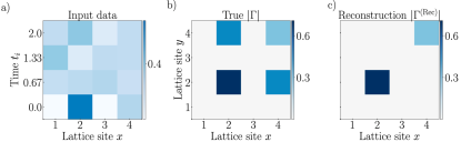
Figure 13: Tomographic recovery of the two site system to a superlattice on four sites. a) The particle number dynamics used as input as shown above does not depend on the complex part of the covariance matrix because we use the nearest-neighbour hopping Hamiltonian $\hat{H}_{\text{NN}}$ with real couplings. b) The absolute value of the covariance matrix. The off-diagonal current is purely imaginary. c) As discussed the imaginary part of the covariance matrix is unconstrained and hence the reconstruction is missing the off-diagonal current. The evolution of the reconstructed covariance matrix yields particle numbers exactly matching the input as proven analytically.

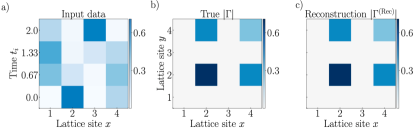
Figure 14: Recovery in the presence of artificial magnetic fields. a) The particle number dynamics is influenced by the complex part of the covariance matrix if we use a Hamiltonian $\hat{H}=\hat{H}_{\text{NN}}+i\sum_{x=1}^{3}\hat{f}^{\dagger}_{x}\hat{f}_{x+1}+\text{h.c}$ with complex couplings. b) The same covariance matrix as above is to be reconstructed. c) The reconstruction now has detected the presence of the complex-valued current.

Appendix E Systematic influence of ramps when quenching many-body interactions

In practice, the switching off of the interactions by means of Feshbach resonances will not be instantaneous. Narrow Feshbach result in relatively fast quenches, and there are no fundamental limits to a fast switching. That said, any switching that is not instantaneous will have some effect. In this section, we discuss the impact of finite ramps, reflecting the process of switching off interactions. Specifically, to provide insight into the resulting effects, we consider the case of fermions with spin and will compute the covariance matrix of thermal states of the Hubbard chain using exact diagonalization. We denote the annihilation operator at $x$ of a spin up fermion by $\hat{f}_{x,\uparrow}$ and for spin down by $\hat{f}_{x,\downarrow}$. In this notation the Hamiltonian of a Hubbard chain on $L$ sites with open boundary conditions reads

$$\hat{H}_{\text{Hubbard}}=-\sum_{\sigma=\uparrow,\downarrow}\sum_{x=1}^{L-1}\hat{f}^{\dagger}_{x,\sigma}\hat{f}_{x+1,\sigma}+\text{h.c.}+U\sum_{x=1}^{L}\hat{N}_{x,\uparrow}\hat{N}_{x,\downarrow}$$ (42)

where $\hat{N}_{x,\sigma}:=\hat{f}^{\dagger}_{x,\sigma}\hat{f}_{x,\sigma}$ for $\sigma=\uparrow,\downarrow$. To ease the notation, we define

$$\hat{a}_{2x-1}:=\hat{f}_{x,\uparrow},\,\,\hat{a}_{2x}:=\hat{f}_{x,\downarrow}$$ (43)

which allows us to concisely write down the Jordan-Wigner transformation

$$\hat{a}_{x}=Z^{\otimes x-1}\otimes S^{-}\otimes\mathds{1}_{2}^{\otimes 2L-x}$$ (44)

with

$$Z=\begin{pmatrix}1&0\\ 0&-1\end{pmatrix}$$ (45)

referring to the Pauli-$z$ matrix and

$$S^{-}=(S^{+})^{\dagger}:=\begin{pmatrix}0&1\\ 0&0\end{pmatrix}.$$ (46)

Using the ordering we have chosen, we find

$$\hat{H}_{\text{Hubbard}}=-\sum_{x=1}^{2L-2}\hat{a}^{\dagger}_{x}\hat{a}_{x+2}+\text{h.c.}+U\sum_{x=1}^{L}\hat{N}_{2x-1}\hat{N}_{2x}$$ (47)

which under the Jordan-Wigner transformation turns into

$$\hat{H}_{\text{Hubbard}}=\sum_{x=1}^{2L-2}S^{+}_{x}Z_{x+1}S^{-}_{x+2}+\text{h.c.}+U\sum_{x=1}^{L}Z_{2x-1}Z_{2x}$$ (48)

where we have used the concise notation

$$\Xi_{x}:=\mathds{1}_{2}^{\otimes x-1}\otimes\Xi\otimes\mathds{1}_{2}^{\otimes 2L-x}$$ (49)

with $\Xi:=Z,S^{+}$ or $S^{-}$. Using exact diagonalization, we compute the thermal density matrix

$$\hat{\varrho}_{\beta}(U)=e^{-\beta\hat{H}_{\text{Hubbard}}}/Z_{\beta}$$ (50)

with $Z_{\beta}:=\operatorname{tr}[e^{-\beta\hat{H}_{\text{Hubbard}}}]$. Using the Jordan-Wigner transformation we then can compute the respective covariance matrix with entries for $x<y$

$$\Gamma^{(\rm Hubbard)}_{x,y} =\operatorname{tr}[\hat{a}_{x}^{\dagger}\hat{a}_{y}\hat{\varrho}_{\beta}(U)]$$ (51)

$$=-\operatorname{tr}[S^{+}_{x}Z_{x+1}\ldots Z_{y-1}S^{-}_{y}\hat{\varrho}_{\beta}(U)].$$

Again using exact diagonalization, we have computed the thermal state for $\beta=3$ and additionally the covariance matrix. The results for the superfluid phase with $U=1$ are shown in Fig. 15 together with a comparison the covariance matrix for just the nearest-neighbour hopping with $U=0$. We find that the difference is very small which means that the Gaussian model is representative for the second moments also of the interacting thermal state if we neglect a small deviation. For this reason the effect of ramping down the interaction in finite time should be less severe because the state will not be strongly affected by it.

For the case of the Mott phase with $U=10$ we find, see Fig. 16, a very substantial difference of the second moments when compared to those obtained from a Gaussian model. To perform a meaningful comparison we consider a heuristic mean-field ansatz for a non-interacting Hamiltonian to yield a Gaussian state to compare to the second moments arising from the interacting Hamiltonian. We chose

$$\hat{H}_{\text{MF},\downarrow}(N^{(\uparrow)})=-\sum_{x=1}^{L}\hat{f}^{\dagger}_{x+1,\downarrow}\hat{f}_{x,\downarrow}+U/8\sum_{x=1}^{L}N^{(\uparrow)}_{x}\hat{N}_{x,\downarrow}$$ (52)

where the spin-up density $UN^{(\uparrow)}/8$ plays the role of a vector of the effective chemical potential for the spin-down band. Qualitatively, the correlations are restricted to nearest neighbour sites while in the non-interacting case they span a larger region. Here a finite duration of ramping down the interaction can sizeably affect the correlations.

The simplest protocol for tomographically reconstructing the second moments $\Gamma^{(U)}$ of an interacting state using our method is to ramp down the interaction in time $T_{\text{Ramp}}$ and at the end of the ramp tilt the optical lattice as explained above. The ramp will have affected the covariance matrix leading to some new second moments $\Gamma^{(U\rightarrow 0)}$ and the tomography will recover these rather than $\Gamma^{(U)}$. The result will hence be accurate if $\Gamma^{(U\rightarrow 0)}\approx\Gamma^{(U)}$. In Fig. 17, we show the effect on the second moments of ramping down the interaction starting from $U=10$ to $U=0$. We depict covariance matrices at the end of ramps of varying length $T_{\text{Ramp}}=0.5,1$ and $2$, so smaller than the tunnelling time, equal, and larger than it. We find that the ramp time does influence the correlations to certain degree but importantly the overall pattern is not overhauled. The changes in the values of the currents increase monotonically with the increase of the duration of the ramp. Due to the limitations of system sizes available in exact diagonalization, we have provided results for only small systems while in the thermodynamical limit one should expect defects appearing due to the Kibble-Zurek mechanism. It seems that it can be avoided, however, by separating a large system into smaller portions such that energy gaps never become smaller than a certain threshold and perform the tomography for each individually. The smaller systems should be larger than the correlation length and such subdivision may be advisable also when dealing with a finite number of total state preparations.

Ramps of this order of duration can be thought of as being implemented by a narrow Feshbach resonance allowing for a relatively fast switching time. With the same approach one could study the case of ramps larger durations but it seems that ramps an order of magnitude longer than the tunnelling time are ill-advised for the sake of correlation read-out using the response to non-interacting dynamics. The reason for this is that for short ramps, as mentioned in the main text, Lieb-Robinson bounds allow to narrow down the influence of the ramp, restricting the action of the its dynamics to the close-by sites and crucially this statement is state independent so can be also employed in cases that are not classically tractable in practice. In contrast, for long ramps, the Lieb-Robinson bounds would not offer a non-trivial estimate of the effect of the ramp.

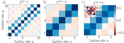
Figure 15: Second moments in the superfluid phase. panel a) shows the covariance matrix of the Hubbard model for $U=1$, panel b) the restriction spin-$\downarrow$ modes. panel c) depicts the covariance matrix of the nearest-neighbour hopping with the same temperature. The inset shows the difference to the covariance matrix of interacting state in absolute values.

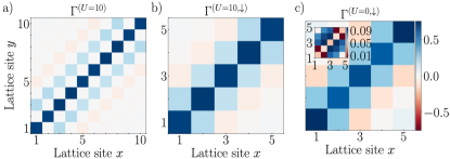
Figure 16: Second moments in the Mott phase. panel a) shows the covariance matrix of the Hubbard model for $U=10$, panel b) the restriction spin-$\downarrow$ modes. panel c) illustrates the covariance matrix of the nearest-neighbour hopping with the same temperature. The inset shows the difference to the covariance matrix of interacting state in absolute values.

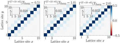
Figure 17: Influence of ramping interactions down in a finite time. We find that the deviation of correlations after the ramp $\Gamma^{(U\rightarrow 0)}$ from the actual second moments $\Gamma^{(U)}$ increase monotonically together with the ramp duration $T_{\text{Ramp}}$ but are small enough such that the correlation patterns are not qualitatively distorted. Hence, we conclude that the tomographic read out would clearly show the effect of the presence of interaction on the second moments and could explore the single-body reduced density matrix for the entire phase diagram of the Hubbard model.

Appendix F Fermionic mode entanglement

In this section, we provide further insights into the operational meaning of the entanglement quantified based on our reconstructions, and what fermionic mode entanglement operationally means. We denote the fermionic Fock state vectors by

$$\left.\left|{\mu}\right.\right\rangle_{\text{F}}:=(\hat{f}^{\dagger}_{1})^{\mu_{1}}\ldots(\hat{f}^{\dagger}_{L})^{\mu_{L}}{\left.\left|{\emptyset}\right.\right\rangle}$$ (53)

with $\mu\in\{0,1\}^{\times L}$ and where ${\left.\left|{\emptyset}\right.\right\rangle}$ denotes the vacuum state vector defined as satisfying $\hat{f}_{x}{\left.\left|{\emptyset}\right.\right\rangle}=0$ for all $x=1,\ldots,L$. For a given order (so basically a symmetric group element $S\in S_{L}$ that captures the order of the fermionic modes when mapping them to spins), we can define a Jordan-Wigner transformation by the relations

$$\hat{f}_{x}=Z^{\otimes x-1}\otimes\begin{pmatrix}0&1\\ 0&0\end{pmatrix}\otimes\mathds{1}_{2}^{\otimes L-x}.$$ (54)

This choice of the Pauli-$z$ matrix fixes its eigenbasis so that we have the convention $Z\left.\left|{\nu}\right.\right\rangle_{\text{S}}=(-1)^{\nu}\left.\left|{\nu}\right.\right\rangle_{\text{S}}$ with $\nu=0,1$ and then Eq. (54) imply directly that

$$\left.\left|{\mu}\right.\right\rangle_{\text{F}}=\otimes_{x=1}^{L}\left.\left|{\mu_{x}}\right.\right\rangle_{\text{S}}.$$ (55)

Note that any ordering of modes can give rise to such a qubit representation where fermionic operators and state vectors can be expressed in an explicit matrix form, but once chosen it should remain fixed throughout calculations. Importantly, occupation states of modes after a non-trivial Bogoliubov transformation will not anymore have such a tensor-product form and one should consider the decomposition into antisymmetric subspaces.

Having fixed the reference ordering of modes, we have a natural notion of fermionic subsystems: A subsystem $A$ consists of a collection of modes, i.e., positions in the lattice, while $B$ is constituted by the complementing modes. In all what follows, we are perfectly free to take the ordering so that modes labeled $1,\dots,|A|$ give rise to subsystem $A$, while $|A|+1,\dots,L$ give rise to $B$.

We now turn to quantum states in such a fermionic setting. Given a quantum state $\hat{\varrho}$ supported on the Hilbert space of the entire system, the reduced state $\hat{\varrho}_{A}$ is defined via functionals of observable algebras: Specifically, it will reflect correlation functions involving operators acting in $A$ equal to those of the global state. That is to say, in what follows, we can treat the system as a system of $|A|$ qubits held by $A$ and $L-|A|$ qubits held by $B$.

Any allowed quantum operation performed within an isolated fermionic system must respect the parity of fermion number super-selection rule Earman (2008); Wick et al. (1952), which implies that at any time, any correlation function involving an odd number of fermionic creation and annihilation operators must vanish. This means that if one performs operations and measurements locally in subsystems $A$ and $B$, then to describe any of such processes it suffices to consider the reduced states $\hat{\varrho}_{A}$ and $\hat{\varrho}_{B}$ to be a direct sum of sectors reflecting even and odd particle numbers in $A$ and $B$, respectively. That is to say, we can first make use of a projection $\pi\otimes\pi$ which projects each of the local subsystems $A$ and $B$ into a direct sum of even and odd particle numbers.

Local operations with classical communication reflecting super-selection rules, referred to as LOCC+SSR, can hence be identified with local operations in the qubit systems reflecting $A$ and $B$ under the Jordan-Wigner transformations, respecting the local direct sum structure of even and odd particle numbers in $A$ and $B$ and the total system. This is a perfectly operational prescription. We call a quantum state mode entangled throughout this article, if it is not a convex combination of uncorrelated quantum states in fermionic modes.

F.1 Single copy fermionic mode entanglement

There is a subtlety arising in the fermionic context, however: This has to do with the presence of super-selection rules. This can be seen as follows. Turning to quantitative prescriptions, one can define single-copy entanglement Nielsen (1999); Eisert and Cramer (2005) as the maximum probability at which one can – at least in principle – extract maximally entangled states of distinguishable quantum systems out of the original system of fermionic modes, making use of any operation in LOCC+SSR that is allowed by quantum mechanics. In this prescription, one may make use of suitable physical interactions or measurements respecting LOCC+SSR. The target distinguishable quantum systems can either be seen as being actually available in the laboratory, e.g., as spin degrees of freedom, or as a conceptual tool to precisely think of mode entanglement in the first place.

Interestingly, in this sense, a state $\hat{\varrho}=\left.\left|{\psi}\right.\right\rangle\left.\left\langle{\psi}\right.\right|$ with $\left.\left|{\psi}\right.\right\rangle=(|0,1\rangle_{\text{F}}+|1,0\rangle_{\text{F}})/\sqrt{2}$ represented as

$$\left.\left|{\Phi}\right.\right\rangle:=\frac{1}{\sqrt{2}}(\left.\left|{0}\right.\right\rangle_{\text{S}}\otimes\left.\left|{1}\right.\right\rangle_{\text{S}}+\left.\left|{1}\right.\right\rangle_{\text{S}}\otimes\left.\left|{0}\right.\right\rangle_{\text{S}})$$ (56)

is not single-copy entangled, as no physically allowed protocol can map this state onto an entangled state of distinguishable quantum systems with any non-zero probability. The projection $\pi$ acting as

$$|\Phi\rangle\langle\Phi|\mapsto(\pi\otimes\pi)|\Phi\rangle\langle\Phi|(\pi\otimes\pi)$$ (57)

will render the state operationally indistinguishable from a quantum state that is merely classically correlated and contains no quantum entanglement. That is to say, for all practical purposes, the state does not contain any entanglement that can be operationally extracted (i.e., with all operations allowed) from a single specimen or copy. It is important to stress that this statement is referring to single-copy entanglement only: It is perfectly an entangled state if asymptotic state transformations are being allowed for, as explained below.

F.2 Distillable fermionic mode entanglement and asymptotic state manipulation

However, the above fermionic two-mode quantum state represented by the state vector $\left.\left|{\psi}\right.\right\rangle=(|0,1\rangle_{\text{F}}+|1,0\rangle_{\text{F}})/\sqrt{2}$ is in fact many-copy entangled, as the SSR is asymptotically not detrimental to the entanglement content of the state vector. Such asymptotic notions involving many copies of identically prepared systems at the same time are the most commonly applied standard notions of entanglement theory, much inspired by notions of classical information theory. Here, one still restricts to quantum operations local to $A$ and $B$, coordinated by classical means by communicating measurement outcomes between $A$ and $B$. But one assumes to have available several copies (or specimens) of the quantum many-body systems available and is allowed to coherently manipulate the quantum state over the copies. Obviously, in practical settings, it is implausible to achieve completely general operations of this kind: It is still a highly convenient abstraction.

The notion of the distillable entanglement Bennett et al. (1996); Horodecki et al. (2009) captures most naturally the resource character of entanglement in quantum information theory. It is in a way the “entanglement content” of a state. It is defined as the optimal rate at which one could extract maximally entangled pairs of distinguishable systems in such a hypothetical optimal state manipulation from many identical copies. This notion not only allows to detect the presence of fermionic entanglement: It also allows to make quantitative estimates, which is precisely what we are interested in here. More precisely and specifically put, the distillable entanglement quantifies the asymptotic rate at which one can extract (“distill”) distinguishable approximately perfect maximally entangled qubit pairs (“Bell pairs”) as in Eq. (56) of distinguishable quantum systems from many identical copies of an input state composed of fermionic modes, using quantum operations from LOCC+SRR Schuch et al. (2004b). For a fermionic initial quantum state $\hat{\varrho}$ on $L$ modes partitioned into $A$ and $B$, the entanglement distillation problem involves as initial state the bona fide quantum state of $n$ copies on $nL$ modes. The final state is asymptotically in $n$ better and better approximating $m$ copies of a maximally entangled pure quantum state associated with the state vector

$$\left.\left|{\psi_{\rm Final}}\right.\right\rangle=\left.\left|{\Phi}\right.\right\rangle^{\otimes m},$$ (58)

in trace-norm $\|.\|_{1}$, so will approximate $m$ Bell pairs. The larger $m$ is, the larger is the yield of this procedure. The distillable entanglement under LOCC+SSR is now

$$E_{D}^{\rm SSR}(\hat{\varrho})=\limsup_{n\rightarrow\infty}\frac{n}{m},$$ (59)

as the supremum over all LOCC+SSR protocols for $n$ input copies and $m$ output copies each. Since the super-selection rule is asymptotically not altering the rate, we have that

$$E_{D}^{\rm SSR}(\hat{\varrho})=E_{D}(\hat{\varrho}),$$ (60)

where the right hand side is the distillable entanglement for the spin equivalent of $\hat{\varrho}$, possibly not respecting super-selection rules Schuch et al. (2004b). The right hand side can be bounded from below by the hashing bound, as stated in the main text. The entanglement cost $E_{C}$ refers to the optimal rate that can be achieved in the converse, starting from $m$ copies of maximally entangled Bell pairs and achieving approximately perfect $n$ copies of the anticipated target state. Again,

$$E_{C}^{\rm SSR}(\hat{\varrho})=E_{C}(\hat{\varrho}),$$ (61)

while in general $E_{C}(\hat{\varrho})\geq E_{D}(\hat{\varrho})$, as the process of distillation can be lossy compared to the process of formation that the entanglement cost captures.

F.3 Evaluation of the witness

We present details on how to evaluate the entanglement witness $E_{G}(\Gamma)$ in this section. We shall make use of the fact that the von Neumann entropy, in general being defined for a quantum state as

$$S(\hat{\varrho})=-\operatorname{tr}[\hat{\varrho}\log(\hat{\varrho})],$$ (62)

is unitarily invariant. For this reason, it can be easily and efficiently be evaluated for a fermionic Gaussian state. In the main text we are using the fact that given the covariance matrix $\Gamma=\Gamma(\hat{\varrho})$ of the state $\hat{\varrho}$, we can associate to the state a unique Gaussian state $\hat{\varrho}^{(\Gamma)}$ with the same second moments. In fact, we have

$$\hat{\varrho}^{(\Gamma)}=\text{argmax}_{\hat{\sigma}}\{S(\hat{\sigma})\text{ s.t. }\Gamma(\hat{\sigma})=\Gamma(\hat{\varrho})\},$$ (63)

which means that Gaussian states give rise to the maximum possible von Neumann entropy, among all quantum states for fixed second moments $\Gamma$ Gluza et al. (2016).

For thermal states of particle number preserving Hamiltonians and for limits of such finite-temperature states, the entropy of a Gaussian state can be computed from the covariance matrix using standard expressions, see, e.g., Refs. Wolf (2006); Peschel (2004), by obtaining the vector $n$ of the eigenvalues of $\Gamma$. We then have

$$S^{(\Gamma)}= S(\hat{\varrho}^{(\Gamma)})=-\sum_{k=1}^{L}f(n_{k}),$$ (64)

where the function $f:[0,1]\rightarrow[0,1]$ is defined as

$$f(x)=\left\{\begin{array}[]{ll}-x\log(x)-(1-x)\log(1-x)\ ,&\text{ if }x>0,\\ 0,&\text{ if }x=0.\\ \end{array}\right.$$ (65)

This formula can be evaluated efficiently in the number of modes. Finally, let us remark that the second moments of a reduced density matrix $\hat{\varrho}_{A}$ describing a subsystem $A$ is obtained by restricting the second moments to $A$ which yields the corresponding covariance matrix $\Gamma_{A}$ and hence for a Gaussian state

$$S(\hat{\varrho}_{A})=S^{(\Gamma_{A})}\ ,$$ (66)

as an expression in terms of the covariance matrix.

F.4 Optimizing the witness value via local Bogoliubov transformations

Our goal is to maximize the witness at hand to achieve the tightest possible lower bound bound. In the main text we gave an example where system $A$ consists of the first 10 modes $A=\{1,2,\ldots,10\}$ and $B=\{11,\ldots,20\}$. If we would apply the witness directly to systems $A$ and $B$ then it will give non-trivial values only for lowest temperatures where the thermal state is very close to the ground state. Indeed, in the case if the global quantum state is pure, then we have $E_{G}(\Gamma)=S^{(\Gamma_{A})}-S^{(\Gamma)}\approx S^{(\Gamma_{A})}$ and whenever the ground state is effectively described by a conformal field theory the subsystem entropy will scale logarithmically in the size of $A$. In the other limit of large temperatures, the entropies of whole system and subsystem $A$ will both scale according to the volume and so the witness will have a negative value. To fix this, one has to make use of the freedom to make local unitary rotations on each subsystem. The goal here is to find some modes that carry only very little entropy such that the witness has a chance to be non-negative.

In general finding the optimal local unitaries that maximize the witness can be complicated but we found that the following heuristic is helpful. Denote by $\Gamma_{A}$ and $\Gamma_{B}$ the principal sub-matrices of $\Gamma$ which are the covariance matrices of subsystems $A$ and $B$ and let $U_{A}$ and $U_{B}$ be the corresponding diagonalization unitaries. Then the Gaussian state $\hat{\varrho}^{\prime}$ with the second moments given by

$$\Gamma^{\prime}=U\Gamma U^{\dagger}=\begin{pmatrix}\Lambda_{A}Q_{A,B}\\ Q_{A,B}^{\dagger}\Lambda_{B}\end{pmatrix}$$ (67)

where $U=U_{A}\oplus U_{B}$, features an identical amount of entanglement because the entanglement cost is invariant under local unitary transformations $E_{C}(\hat{\varrho})=E_{C}(\hat{\varrho}^{\prime})$. We hence can focus on the quantum state $\hat{\varrho}^{\prime}$.

We observe that this is a viable distillation heuristic, as now there can be a mode $a\in A$ and a mode $b\in B$ such that their covariance matrix $\Gamma^{\prime}_{\{a,b\}}$ features a larger purity than before. This is the meaning of the sparse off-diagonal structure seen in the figure presented in the main text. We can restrict to these modes because entanglement cost is monotonous under partial traces

$$E_{C}(\hat{\varrho}^{\prime})\geq E_{C}(\hat{\varrho}^{\prime}_{a,b}),$$ (68)

i.e., discarding some degrees of freedom can only decrease the available entanglement resources. This discarding however is crucial because we get a better chance for the witness value to be non-trivial – for this the discarded modes should take away most of the entropy while the reduced state of the remaining modes should be as pure as possible.

References

- Bloch et al. (2012) I. Bloch, J. Dalibard, and S. Nascimbene, Nature Phys. 8, 267 (2012).
- Greiner et al. (2001) M. Greiner, I. Bloch, O. Mandel, T. W. Hänsch, and T. Esslinger, Phys. Rev. Lett. 87, 160405 (2001).
- Endres et al. (2011) M. Endres, M. Cheneau, T. Fukuhara, C. Weitenberg, P. Schauss, C. Gross, L. Mazza, M. C. Banuls, L. Pollet, I. Bloch, and S. Kuhr, Science 334, 200 (2011).
- Tai et al. (2017) M. E. Tai, A. Lukin, M. Rispoli, R. Schittko, T. Menke, D. Borgnia, P. M. Preiss, F. Grusdt, A. M. Kaufman, and M. Greiner, Nature 546, 519 (2017).
- Trotzky et al. (2010) S. Trotzky, L. Pollet, F. Gerbier, U. Schnorrberger, I. Bloch, N. Prokof’ev, B. Svistunov, and M. Troyer, Nature Phys. 6, 998 (2010).
- Trotzky et al. (2012) S. Trotzky, Y.-A. Chen, A. Flesch, I. P. McCulloch, U. Schollwöck, J. Eisert, and I. Bloch, Nature Phys. 8, 325 (2012).
- Kaufman et al. (2016) A. M. Kaufman, M. E. Tai, A. Lukin, M. Rispoli, R. Schittko, P. M. Preiss, and M. Greiner, Science 353, 794 (2016).
- Braun et al. (2015) S. Braun, M. Friesdorf, S. S. Hodgman, M. Schreiber, J. P. P. Ronzheimer, A. Riera, M. del Rey, I. Bloch, J. Eisert, and U. Schneider, Proc. Natl. Ac. Sc. 112, 3641 (2015).
- Ronzheimer et al. (2013) J. P. Ronzheimer, M. Schreiber, S. Braun, S. S. Hodgman, S. Langer, I. P. McCulloch, F. Heidrich-Meisner, I. Bloch, and U. Schneider, Phys. Rev. Lett. 110, 205301 (2013).
- Hofferberth et al. (2007) S. Hofferberth, I. Lesanovsky, B. Fischer, T. Schumm, and J. Schmiedmayer, Nature 449, 324 (2007).
- Gring et al. (2012) M. Gring, M. Kuhnert, T. Langen, T. Kitagawa, B. Rauer, M. Schreitl, I. Mazets, D. A. Smith, E. Demler, and J. Schmiedmayer, Science 337, 1318 (2012).
- Langen et al. (2015) T. Langen, S. Erne, R. Geiger, B. Rauer, T. Schweigler, M. Kuhnert, W. Rohringer, I. E. Mazets, T. Gasenzer, and J. Schmiedmayer, Science 348, 207 (2015).
- Cheneau et al. (2012) M. Cheneau, P. Barmettler, D. Poletti, M. Endres, P. Schauss, T. Fukuhara, C. Gross, I. Bloch, C. Kollath, and S. Kuhr, Nature 481, 484 (2012).
- Schweigler et al. (2017) T. Schweigler, V. Kasper, S. Erne, I. E. Mazets, B. Rauer, F. Cataldini, T. Langen, T. Gasenzer, J. Berges, and J. Schmiedmayer, Nature 545, 323 (2017).
- Acin et al. (2018) A. Acin, I. Bloch, H. Buhrman, T. Calarco, C. Eichler, J. Eisert, D. Esteve, N. Gisin, S. J. Glaser, F. Jelezko, S. Kuhr, M. Lewenstein, M. F. Riedel, P. O. Schmidt, R. Thew, A. Wallraff, I. Walmsley, and F. K. Wilhelm, New J. Phys. 20, 080201 (2018).
- Mazurenko et al. (2017) A. Mazurenko, C. S. Chiu, G. Ji, M. F. Parsons, M. Kanasz-Nagy, R. Schmidt, F. G. E., Demler, , Greif, and M. Greiner, Nature 545, 462 (2017).
- Köhl et al. (2005) M. Köhl, H. Moritz, T. Stöferle, K. Günter, and T. Esslinger, Phys. Rev. Lett. 94, 080403 (2005).
- Esslinger (2010) T. Esslinger, Ann. Rev. Con and Mat. Phys. 1, 129 (2010).
- Schneider et al. (2012) U. Schneider, L. Hackermüller, J. P. Ronzheimer, S. Will, T. B. S. Braun, I. Bloch, E. Demler, S. Mandt, D. Rasch, and A. Rosch, Nature Phys. 8, 213 (2012).
- Rom et al. (2006) T. Rom, T. Best, D. van Oosten, U. Schneider, S. Foelling, B. Paredes, and I. Bloch, Nature 444, 733 (2006).
- Chiu et al. (2018) C. S. Chiu, G. Ji, A. Mazurenko, D. Greif, and M. Greiner, Phys. Rev. Lett. 120, 243201 (2018).
- Behrle et al. (2018) A. Behrle, T. Harrison, J. Kombe, K. Gao, M. Link, J.-S. Bernier, C. Kollath, and M. Köhl, Nature Phys. 14, 781 (2018).
- Viebahn et al. (2019) K. Viebahn, M. Sbroscia, E. Carter, J.-C. Yu, and U. Schneider, Phys. Rev. Lett. 122, 110404 (2019).
- Chiu et al. (2019) C. S. Chiu, G. Ji, A. Bohrdt, M. Xu, M. Knap, E. Demler, F. Grusdt, M. Greiner, and D. Greif, Science 365, 251 (2019).
- Yang et al. (2020) B. Yang, H. Sun, C.-J. Huang, H.-Y. Wang, Y. Deng, H.-N. Dai, Z.-S. Yuan, and J.-W. Pan, Science 369, 550 (2020).
- Eisert et al. (2020) J. Eisert, D. Hangleiter, N. Walk, I. Roth, D. Markham, R. Parekh, U. Chabaud, and E. Kashefi, Nature Rev. Phys. 2, 382 (2020).
- Sherson et al. (2010) J. F. Sherson, C. Weitenberg, M. Endres, M. Cheneau, I. Bloch, and S. Kuhr, Nature 467, 68 (2010).
- Bakr et al. (2010) W. S. Bakr, A. Peng, M. E. Tai, R. Ma, J. Simon, J. I. Gillen, S. Fölling, L. Pollet, and M. Greiner, Science 329, 547 (2010).
- Weitenberg et al. (2011) C. Weitenberg, M. Endres, J. F. Sherson, M. Cheneau, P. Schauß, T. Fukuhara, I. Bloch, and S. Kuhr, Nature 471, 319 (2011).
- Eisert et al. (2015) J. Eisert, M. Friesdorf, and C. Gogolin, Nature Phys. 11, 124 (2015).
- Schreiber et al. (2015) M. Schreiber, S. S. Hodgman, P. Bordia, H. P. Lüschen, M. H. Fischer, R. Vosk, E. Altman, U. Schneider, and I. Bloch, Science 349, 842 (2015).
- Bergschneider et al. (2019) A. Bergschneider, V. M. Klinkhamer, J. H. Becher, R. Klemt, L. Palm, G. Zürn, S. Jochim, and P. M. Preiss, Nature Physics 15, 640 (2019).
- Gluza et al. (2020) M. Gluza, T. Schweigler, B. Rauer, C. Krumnow, J. Schmiedmayer, and J. Eisert, Comm. Phys. 3, 12 (2020).
- Ohliger et al. (2013) M. Ohliger, V. Nesme, and J. Eisert, New J. Phys. 15, 015024 (2013).
- Merkel et al. (2010) S. T. Merkel, C. A. Riofrío, S. T. Flammia, and I. H. Deutsch, Phys. Rev. A 81, 032126 (2010).
- Elben et al. (2018) A. Elben, B. Vermersch, M. Dalmonte, J. I. Cirac, and P. Zoller, Phys. Rev. Lett. 120, 050406 (2018).
- Hauke et al. (2014) P. Hauke, M. Lewenstein, and A. Eckardt, Phys. Rev. Lett. 113, 045303 (2014).
- Pena Ardila et al. (2018) L. A. Pena Ardila, M. Heyl, and A. Eckardt, Phys. Rev. Lett. 121, 260401 (2018).
- Qin et al. (2018) T. Qin, A. Schnell, K. Sengstock, C. Weitenberg, A. Eckardt, and W. Hofstetter, arXiv preprint arXiv:1804.03200 (2018).
- Tarnowski et al. (2017) M. Tarnowski, F. N. Ünal, N. Fläschner, B. S. Rem, A. Eckardt, K. Sengstock, and C. Weitenberg, arXiv:1709.01046 (2017).
- Keßler and Marquardt (2014) S. Keßler and F. Marquardt, Phys. Rev. A 89, 061601 (2014).
- Loida et al. (2018) K. Loida, J.-S. Bernier, R. Citro, E. Orignac, and C. Kollath, Phys. Rev. A 98, 033605 (2018).
- Atala et al. (2014) M. Atala, M. Aidelsburger, M. Lohse, J. T. Barreiro, B. Paredes, and I. Bloch, Nature Physics 10, 588 (2014).
- Schweizer et al. (2016) C. Schweizer, M. Lohse, R. Citro, and I. Bloch, Phys. Rev. Lett. 117, 170405 (2016).
- Huang et al. (2020) H.-Y. Huang, R. Kueng, and J. Preskill, Nature Phys. (2020).
- Diamond and Boyd (2016) S. Diamond and S. Boyd, J. Mach. Learn. Res. 17, 1 (2016).
- (47) M. Gluza, The numerical code is freely available at https://github.com/marekgluza/hopping_tomography and includes interactive Python notebooks allowing to reproduce the figures.
- Preiss et al. (2015) P. M. Preiss, R. Ma, M. E. Tai, A. Lukin, M. Rispoli, P. Zupancic, Y. Lahini, R. Islam, and M. Greiner, Science 347, 1229 (2015).
- Rauer et al. (2018) B. Rauer, S. Erne, T. Schweigler, F. Cataldini, M. Tajik, and J. Schmiedmayer, Science 360, 307 (2018).
- Lieb and Robinson (1972) E. H. Lieb and D. W. Robinson, Commun. Math. Phys. 28, 251 (1972).
- Hartke et al. (2020) T. Hartke, B. Oreg, N. Jia, and M. Zwierlein, Phys. Rev. Lett. 125, 113601 (2020).
- Nichols et al. (2019) M. A. Nichols, L. W. Cheuk, M. Okan, T. R. Hartke, E. Mendez, T. Senthil, E. Khatami, H. Zhang, and M. W. Zwierlein, Science 363, 383 (2019).
- Brown et al. (2019) P. T. Brown, D. Mitra, E. Guardado-Sanchez, R. Nourafkan, A. Reymbaut, C.-D. Hébert, S. Bergeron, A.-M. S. Tremblay, J. Kokalj, D. A. Huse, P. Schauß, and W. S. Bakr, Science 363, 379 (2019).
- Takasu et al. (2020) Y. Takasu, T. Yagami, H. Asaka, Y. Fukushima, K. Nagao, S. Goto, I. Danshita, and Y. Takahashi, Science Advances 6 (2020), 10.1126/sciadv.aba9255.
- Nakamura et al. (2019) Y. Nakamura, Y. Takasu, J. Kobayashi, H. Asaka, Y. Fukushima, K. Inaba, M. Yamashita, and Y. Takahashi, Phys. Rev. A 99, 033609 (2019).
- Cocchi et al. (2017) E. Cocchi, L. A. Miller, J. H. Drewes, C. F. Chan, D. Pertot, F. Brennecke, and M. Köhl, Phys. Rev. X 7, 031025 (2017).
- Chan et al. (2020) C. F. Chan, M. Gall, N. Wurz, and M. Köhl, Phys. Rev. Research 2, 023210 (2020).
- Guardado-Sanchez et al. (2020) E. Guardado-Sanchez, A. Morningstar, B. M. Spar, P. T. Brown, D. A. Huse, and W. S. Bakr, Phys. Rev. X 10, 011042 (2020).
- Kokail et al. (2019) C. Kokail, C. Maier, R. van Bijnen, T. Brydges, M. K. Joshi, P. Jurcevic, C. A. Muschik, P. Silvi, R. Blatt, C. F. Roos, et al., Nature 569, 355 (2019).
- Bennett et al. (1996) C. H. Bennett, H. J. Bernstein, S. Popescu, and B. Schumacher, Phys. Rev. A 53, 2046 (1996).
- Horodecki et al. (2009) R. Horodecki, P. Horodecki, M. Horodecki, and K. Horodecki, Rev. Mod. Phys. 81, 865 (2009).
- Eisert et al. (2007) J. Eisert, F. G. Brandao, and K. M. Audenaert, New J. Phys. 9 (2007).
- Audenaert and Plenio (2006) K. M. R. Audenaert and M. B. Plenio, New J. Phys. 8, 266 (2006).
- Guehne et al. (2007) O. Guehne, M. Reimpell, and R. F. Werner, Phys. Rev. Lett. 98, 110502 (2007).
- Cramer et al. (2013) M. Cramer, A. Bernard, N. Fabbri, L. Fallani, C. Fort, S. Rosi, F. Caruso, M. Inguscio, and M. Plenio, Nature Comm. 4, 3161 (2013).
- Earman (2008) J. Earman, Erkenntnis 69, 377 (2008).
- Wick et al. (1952) G. C. Wick, A. S. Wightman, and E. P. Wigner, Phys. Rev. 88, 101 (1952).
- Schuch et al. (2004a) N. Schuch, F. Verstraete, and J. I. Cirac, Phys. Rev. A 70, 042310 (2004a).
- Devetak and Winter (2005) I. Devetak and A. Winter, Proc. R. Soc. Lon and A 461, 207 (2005).
- Pastawski et al. (2017) F. Pastawski, J. Eisert, and H. Wilming, Phys. Rev. Lett. 119, 020501 (2017).
- Eisert and Wolf (2007) J. Eisert and M. W. Wolf, “Gaussian quantum channels,” in Quantum Information with Continous Variables of Atoms and Light (Imperial College Press, London, 2007) pp. 23–42, arXiv:quant-ph/0505151.
- Kraus and Cirac (2010) C. V. Kraus and J. I. Cirac, New J. Phys. 12, 113004 (2010).
- Brydges et al. (2019) T. Brydges, A. Elben, P. Jurcevic, B. Vermersch, C. Maier, B. P. Lanyon, P. Zoller, R. Blatt, and C. F. Roos, Science 364, 260 (2019).
- Hastings and Koma (2006) M. B. Hastings and T. Koma, Commun. Math. Phys. 265, 781 (2006).
- Bera et al. (2015) S. Bera, H. Schomerus, F. Heidrich-Meisner, and J. H. Bardarson, Phys. Rev. Lett. 115, 046603 (2015).
- Gluza et al. (2018) M. Gluza, M. Kliesch, J. Eisert, and L. Aolita, Phys. Rev. Lett. 120, 190501 (2018).
- Arute et al. (2020) F. Arute, K. Arya, R. Babbush, D. Bacon, J. C. Bardin, R. Barends, S. Boixo, M. Broughton, B. B. Buckley, D. A. Buell, et al., arXiv:2004.04174 (2020).
- Flammia and Liu (2011) S. T. Flammia and Y.-K. Liu, Phys. Rev. Lett. 106, 230501 (2011).
- Nielsen (1999) M. A. Nielsen, Phys. Rev. Lett. 83, 436 (1999).
- Eisert and Cramer (2005) J. Eisert and M. Cramer, Phys. Rev. A 72, 042112 (2005).
- Schuch et al. (2004b) N. Schuch, F. Verstraete, and J. I. Cirac, Phys. Rev. A 70, 042310 (2004b).
- Gluza et al. (2016) M. Gluza, C. Krumnow, M. Friesdorf, C. Gogolin, and J. Eisert, Phys. Rev. Lett. 117, 190602 (2016).
- Wolf (2006) M. M. Wolf, Phys. Rev. Lett. 96, 010404 (2006).
- Peschel (2004) I. Peschel, J. Stat. Mech. , P12005 (2004).