Topological terms on topological defects: a quantum Monte Carlo study

Abstract

Dirac fermions in $2+1$ dimensions with dynamically generated anticommuting SO(3) antiferromagnetic (AFM) and Z₂ Kekulé valence-bond solid (KVBS) masses map onto a field theory with a topological $\theta$-term. This term provides a mechanism for continuous phase transitions between different symmetry-broken states: topological defects of one phase carry the charge of the other and proliferate at the transition. The $\theta$-term implies that a domain wall of the Z₂ KVBS order parameter harbors a spin-$1/2$ Heisenberg chain, as described by a $1+1$ dimensional SO(3) non-linear sigma model with $\theta$-term at $\theta=\pi$. Using pinning fields to stabilize the domain wall, we show that our auxiliary-field quantum Monte Carlo simulations indeed support the emergence of a spin-$1/2$ chain at the Z₂ topological defect. This concept can be generalized to higher dimensions where $2+1$ dimensional SO(4) or SO(5) theories with topological terms are realized at a domain wall.

Introduction.—Topological terms in field theories play an important role in our understanding of phases and critical phenomena. For instance, the differences between integer and half-integer spin-$S$ chains are a consequence of the $2\pi iS$ pre-factor of the integer-valued $\theta$-term that counts the winding of a unit vector over the sphere. Dirac fermions provide a very appealing route to define models that map onto field theories with topological terms [1; 2; 3; 4; 5; 6; 7; 8; 9]. Consider 8-flavored Dirac fermions in $2+1$ dimensions akin to graphene. In this case, there is a maximum of five anti-commuting mass terms that could, for instance, correspond to an antiferromagnet (AFM) with three mass terms and a Kekulé valence bond solid (KVBS) with two mass terms [10]. The ten commutators of these mass terms correspond to the generators of the SO(5) group so that Dirac fermions Yukawa-coupled to these five mass terms possess an SO(5) symmetry. In the massive phase, one can integrate out the fermions to obtain a Wess-Zumino-Witten (WZW) topological term [1; 2] that is believed to be at the origin of deconfined quantum criticality (DQC) [11; 12]. In particular, it formalizes the Levin-Senthil picture [13] of a vortex of the Kekulé order harboring an emergent spin-$1/2$ degree of freedom.

The aim of this Letter is to demonstrate numerically the consequences of topological terms in the corresponding field theory. We will do so by considering a model of Dirac fermions in 2+1 dimensions with reduced spatial symmetries such that the three AFM and one of the two KVBS mass terms are dynamically generated. Contrary to the generic KVBS state with a spontaneously broken U(1) symmetry in the continuum, our KVBS state spontaneously breaks a Z₂ symmetry. We will refer to this state as Z₂ KVBS. Starting from the WZW topological term, this symmetry reduction amounts to setting one component of the five-dimensional field to zero. This maps the WZW term to a $\theta$-term at $\theta=\pi$ [3]. Let us assume that the phase transition observed numerically between the AFM and the Z₂ KVBS is continuous and captured by the aforementioned field theory. Then, the $\theta$-term leads to the prediction that in the Z₂ KVBS phase close to the transition, a Z₂ KVBS domain wall harbors a spin-$1/2$ chain. In what follows, we will provide a model—amenable to large scale negative-sign-free auxiliary-field quantum Monte Carlo (QMC) calculations—that provides compelling results supporting this field-theory picture.

Field theory.—A theory that accounts for the phase diagram presented in Ref. [6] (see Fig. 1(a)) contains Dirac fermions Yukawa-coupled to the AFM and Z₂ KVBS mass terms, as described by

$${\cal L}_{\text{F}} ={\Psi}^{\dagger}\left[\partial_{\mu}(\boldsymbol{1}_{2}\otimes\gamma_{0}\gamma_{\mu})+\begin{pmatrix}\eta_{\alpha}\\ \chi\end{pmatrix}\cdot\begin{pmatrix}{\sigma}_{\alpha}\otimes\gamma_{0}\\ \boldsymbol{1}_{2}\otimes i\gamma_{0}\gamma_{5}\end{pmatrix}\right]{\Psi}^{\phantom{\dagger}}.$$

Here, the Dirac spinors ${\Psi}^{\dagger}$ carry a sublattice index, a spin index, and a valley index. The $\gamma$-matrices act on the valley and sublattice spaces and satisfy the Clifford algebra $\{\gamma_{a},\gamma_{b}\}=2\delta_{ab}$. ${\sigma}_{\alpha}$ with $\alpha=1,2,3$ denote the Pauli spin-$1/2$ matrices. The fact that the SO(3) AFM mass terms ${\sigma}_{\alpha}\otimes\gamma_{0}$ and Z₂ KVBS mass terms $\boldsymbol{1}_{2}\otimes i\gamma_{0}\gamma_{5}$ anti-commute results in an SO(4) invariance of the fermionic action: a global SO(4) rotation of the four-component field $\boldsymbol{\phi}=(\phi_{1},\phi_{2},\phi_{3},\phi_{4})=(\boldsymbol{\eta},\chi)$ is equivalent to a canonical transformation of the fermion operators. The dynamics of the field is governed by a four-component $\varphi^{4}$ action, ${\cal L}_{\text{B}}$. While ${\cal L}_{\text{F}}$ has SO(4) symmetry, ${\cal L}_{\text{B}}$ inherits the SO(3) $\times$ Z₂ symmetry of the lattice model.

The Lagrangian ${\cal L}={\cal L}_{\text{F}}+{\cal L}_{\text{B}}$ can account for many phase transitions. The Gross-Neveu transitions from semimetal to AFM or from semimetal to Z₂ KVBS involve a closing of the mass gap corresponding to the norm of the field $\boldsymbol{\phi}$. On the other hand, QMC simulations (see Ref. [6] and the Supplemental Material (SM)) point to a continuous transition between the AFM and Z₂ KVBS states with an emergent SO(4) symmetry. Importantly, the numerical results show that the single-particle gap remains finite across the transition. In the field theory, this implies that amplitude fluctuations of $\boldsymbol{\phi}$ are frozen and only phase fluctuations of the field need to be retained. Since the fermions remain massive, they can be integrated out (in the large mass limit) to obtain

$$S=\int dx^{2}d\tau\frac{1}{g}(\partial_{u}\hat{\boldsymbol{\phi}})^{2}+i\theta{\cal Q}~{}~{},~{}~{}\theta=\pi$$ (2)

with

$${\cal Q}=\frac{1}{12\pi^{2}}\int dx^{2}d\tau\epsilon_{i,j,k}\epsilon_{\alpha,\beta,\gamma,\delta}\hat{{\phi}}_{\alpha}\partial_{i}\hat{{\phi}}_{\beta}\partial_{j}\hat{{\phi}}_{\gamma}\partial_{k}\hat{{\phi}}_{\delta}.$$ (3)

Here, $\hat{\boldsymbol{\phi}}(\boldsymbol{x},\tau)=\boldsymbol{\phi}/|\boldsymbol{\phi}|$ defines a mapping from $2+1$ dimensional Euclidean space-time to the three-dimensional sphere $S^{3}$. For smooth field configurations with no singularities at infinity ${\cal Q}$ is quantized to integer values and corresponds to the winding of the unit four-vector $\hat{\boldsymbol{\phi}}$ on the hypersphere in four dimensions, $S^{3}$.

We now consider a smooth domain wall of the Z₂ KVBS order parameter. Such a configuration can be obtained by pinning the field $\hat{\boldsymbol{\phi}}$ at the origin and at infinity: $\hat{\boldsymbol{\phi}}(\boldsymbol{0})=(0,0,0,1)$ and $\hat{\boldsymbol{\phi}}(\boldsymbol{\infty})=(0,0,0,-1)$. Specifically, let us parameterize 2+1 dimensional Euclidean space-time with spherical coordinates, $(\boldsymbol{x},\tau)=r\boldsymbol{n}$ with $\boldsymbol{n}$ a unit vector, and choose

$$\hat{\phi}(r\boldsymbol{n})=\left(\sin(f(r))\boldsymbol{n},\cos(f(r)\right).$$ (4)

Here, $f$ is a one-to-one smooth function with boundary conditions $f(0)=0$ and $f(\infty)=\pi$ and describes the profile of the domain wall. As shown in the SM, the integration over $r$ can now be carried out to obtain the domain-wall action:

$$S_{DW}=\int dxd\tau\frac{1}{g}(\partial_{u}\boldsymbol{n})^{2}+i\pi{\cal Q}_{DW}(\boldsymbol{n})$$ (5)

with

$${\cal Q}_{DW}(\boldsymbol{n})=\frac{1}{4\pi}\int dxd\tau\boldsymbol{n}\cdot\partial_{\tau}\boldsymbol{n}\times\partial_{x}\boldsymbol{n}.$$ (6)

Above we have mapped $S^{2}$ (on which $\boldsymbol{n}$ is defined) to $\mathbb{R}^{2}$. While the topological term is independent of the choice of the profile of the domain wall, $g$ depends on $f$. The action in Eq. (5) corresponds to that of the spin-$1/2$ Heisenberg chain [14; 15]. Thereby, the topological $\theta$-term at $\theta=\pi$ has the important consequence that a domain wall of the Z₂ KVBS order parameter harbors a spin-$1/2$ Heisenberg chain.

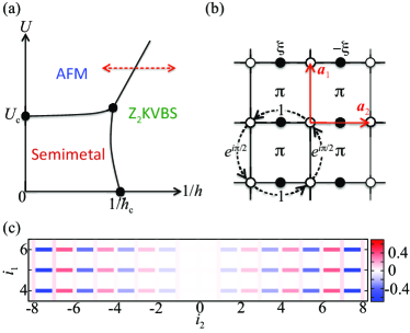
Figure 1: (a) Schematic ground-state phase diagram with semimetallic, AFM, and Z₂ KVBS phases [6]. Results correspond to scans along the dashed line. (b) In our model, fermions acquire a $\pi$-flux when circulating around a plaquette. Bonds labeled by a solid circle accommodate an Ising spin that couples to the fermions with magnitude $\pm\xi$. We consider periodic (open) boundary conditions in the $\boldsymbol{a}_{1}$ ($\boldsymbol{a}_{2}$) directions and freeze the Ising spins on the open boundary to impose a domain wall. (c) Real-space bond energy change $\Delta\hat{B}_{\boldsymbol{i},\boldsymbol{a}_{l}}$ (see text). Here, $L_{1}=30$ and $L_{2}=17$.

Model.—The QMC simulations presented in Ref. [6] for the honeycomb lattice support a direct and continuous transition between the AFM and Z₂ KVBS with an emergent SO(4) symmetry and, in principle, provide a case to test the above predictions. However, irrespective of how one places the pinning fields on the honeycomb lattice, translation symmetry along the domain wall will be broken. Since gaplessness of the spin-$1/2$ chain is protected by a mixed anomaly between translations and time-reversal or spin rotations, dimerization along the domain wall will occur. Hence, even if a spin chain emerges at the domain wall, it will gap out due to the choice of lattice discretization. To avoid this, we have reformulated the model of Ref. [6] on the $\pi$-flux square lattice. This provides a lattice discretization of Dirac fermions with a C₄ symmetry (as opposed to C₃ for the honeycomb lattice). The model Hamiltonian reads $\hat{H}=\hat{H}_{\text{f}}+\hat{H}_{\text{s}}+\hat{H}_{\text{fs}}$ (see Fig. 1(b)) with

$$\hat{H}_{\text{f}} =\sum_{\langle\boldsymbol{ij}\rangle,\sigma}t_{\boldsymbol{ij}}\hat{c}_{\boldsymbol{i}\sigma}^{\dagger}\hat{c}_{\boldsymbol{j}\sigma}+U\sum_{\boldsymbol{i}}(\hat{n}_{\boldsymbol{i}\uparrow}-\mbox{$\frac{1}{2}$})(\hat{n}_{\boldsymbol{i}\downarrow}-\mbox{$\frac{1}{2}$}),$$ (7)

$$\hat{H}_{\text{s}} =J\sum_{\langle\boldsymbol{ij,kl}\rangle}\hat{s}_{\boldsymbol{ij}}^{z}\hat{s}_{\boldsymbol{kl}}^{z}-h\sum_{\langle\boldsymbol{ij}\rangle}\hat{s}_{\boldsymbol{ij}}^{x},\,\,\,\hat{H}_{\text{fs}}=\sum_{\langle\boldsymbol{ij}\rangle,\sigma}t_{\boldsymbol{ij}}\xi_{\boldsymbol{ij}}\hat{s}_{\boldsymbol{ij}}^{z}\hat{c}_{\boldsymbol{i}\sigma}^{\dagger}\hat{c}_{\boldsymbol{j}\sigma}.$$

While $\hat{H}_{\text{f}}$ corresponds to the half-filled Hubbard model on the $\pi$-flux square lattice, $\hat{H}_{\text{s}}$ is a ferromagnetic, transverse-field Ising model defined on the bonds $\langle\boldsymbol{ij}\rangle$ of the square lattice. $\hat{H}_{\text{fs}}$ accounts for the coupling between Dirac fermions and Ising spins. The Hubbard interaction and the fermion-spin coupling can dynamically generate SO(3) AFM order and Z₂ KVBS order (ferromagnetic order of the Ising spins), respectively. For the numerical simulations we used the ALF (Algorithms for Lattice Fermions) implementation [16] of the well-established finite-temperature auxiliary-field QMC method [17; 18]. Our model can be simulated without encountering the negative sign problem. Henceforth, we use $t=1$ as the energy unit, set $J=-1$, $\xi=0.5$, and $U=7$. An inverse temperature $\beta=30$ (with Trotter discretization $\Delta\tau=0.1$) yields results representative of the ground state. QMC results on torus geometries detailed in the SM suggest a continuous AFM–Z₂ KVBS transition with emergent SO(4) symmetry at $1/h_{c}\approx 0.270$.

To pin a domain wall configuration, we consider a cylindrical geometry and freeze the Ising spins at the edges to $\hat{s}_{(i_{1},-n),(i_{1},-n+1)}^{z}=1$ and $\hat{s}_{(i_{1},n-1),(i_{1},n)}^{z}=-1$ where $L_{2}=2n+1$. Importantly, and taking into account the gauge freedom to define the $\pi$-flux model, translation symmetry by $\boldsymbol{a}_{1}$ is present. The model with pinning fields has a mirror symmetry corresponding to the combined transformations $\hat{c}_{(i_{1},i_{2}),\sigma}^{\dagger}\to\hat{c}_{(i_{1},-i_{2}),\sigma}^{\dagger}$ and $\hat{s}_{(i_{1},i_{2}),(i_{1},i_{2}+1)}^{z}\to-\hat{s}_{(i_{1},i_{2}),(i_{1},-i_{2}-1)}^{z}$.

Numerical results.—To detect the profile of the domain wall, we measure the bond kinetic energy $\Delta\hat{B}_{\boldsymbol{i},\boldsymbol{a}_{l}}=\langle\hat{B}_{\boldsymbol{i},\boldsymbol{a}_{l}}\rangle-\langle\bar{B}\rangle$. Here, $\hat{B}_{\boldsymbol{i},\boldsymbol{a}_{l}}=\sum_{\sigma}t_{\boldsymbol{i},\boldsymbol{i}+\boldsymbol{a}_{l}}(\hat{c}_{\boldsymbol{i}\sigma}^{\dagger}\hat{c}_{\boldsymbol{i}+\boldsymbol{a}_{l}\sigma}+\hat{c}_{\boldsymbol{i+\boldsymbol{a}_{l}}\sigma}^{\dagger}\hat{c}_{\boldsymbol{i}\sigma})$ and $\bar{B}=(2L_{1}L_{2})^{-1}\sum_{\boldsymbol{i},l}\hat{B}_{\boldsymbol{i},\boldsymbol{a}_{l}}$ where $l=1,2$. Figure 1(c) shows this quantity. The aforementioned translation and mirror symmetries are readily seen.

As discussed above, the field theory of the domain wall is described by an SO(3) non-linear sigma model with $\theta$-term at $\theta=\pi$ in 1+1 dimensions. We expect this theory to have an emergent SO(4) [19; 20] symmetry reflecting the fact that spin-spin and dimer-dimer correlations decay with the same power law but with different logarithmic corrections: $(-1)^{r}(\ln{r})^{1/2}r^{-1}$ for the spin  [21; 22; 23] and $(-1)^{r}(\ln{r})^{-3/2}r^{-1}$ for the dimer  [23]. In Figs. 2(a-c) we plot the spin [$C^{S}(\boldsymbol{i})=\langle\hat{\boldsymbol{S}}_{\boldsymbol{i}}\cdot\hat{\boldsymbol{S}}_{\boldsymbol{0}}\rangle$], dimer [$C^{D}(\boldsymbol{i})=\langle(\hat{\boldsymbol{D}}_{\boldsymbol{i}}-\langle\hat{\boldsymbol{D}}_{\boldsymbol{i}}\rangle)\cdot(\hat{\boldsymbol{D}}_{\boldsymbol{0}}-\langle\hat{\boldsymbol{D}}_{\boldsymbol{0}}\rangle)\rangle$] and bond [$C^{B}(\boldsymbol{i})=\langle(\hat{B}_{\boldsymbol{i},\boldsymbol{a}_{1}}-\langle\hat{B}_{\boldsymbol{i},\boldsymbol{a}_{1}}\rangle)\cdot(\hat{B}_{\boldsymbol{0},\boldsymbol{a}_{1}}-\langle\hat{B}_{\boldsymbol{0},\boldsymbol{a}_{1}}\rangle)\rangle$] correlators as a function of the conformal distance $x=L_{1}{\rm sin}(\pi i_{1}/L_{1})$ [24]. Here, $\hat{\boldsymbol{S}}_{\boldsymbol{i}}=\sum_{\sigma\sigma^{\prime}}\hat{c}_{\boldsymbol{i}\sigma}^{\dagger}\boldsymbol{\sigma}_{\sigma\sigma^{\prime}}\hat{c}_{\boldsymbol{i}\sigma^{\prime}}$, and $\hat{\boldsymbol{D}}_{\boldsymbol{i}}=\hat{\boldsymbol{S}}_{\boldsymbol{i}}\cdot\hat{\boldsymbol{S}}_{\boldsymbol{i}+\boldsymbol{a}_{1}}$. The bond and dimer correlations share the same symmetries so that we expect them to decay with the same power law. We compare our results with those for the half-filled Hubbard chain at $U/t=4$. While there is remarkable agreement between the spin correlations (see Fig. 2(a)) it appears that we have to reach longer length scales in the domain wall calculation to observe the $1/r$ power law decay for the dimer and bond correlations (see Fig. 2(b),(c)). A possible interpretation of these numerical results is that the Hubbard model is closer to the emergent SO(4) conformal field theory than the domain wall SO(3) theory of Eq. (5).

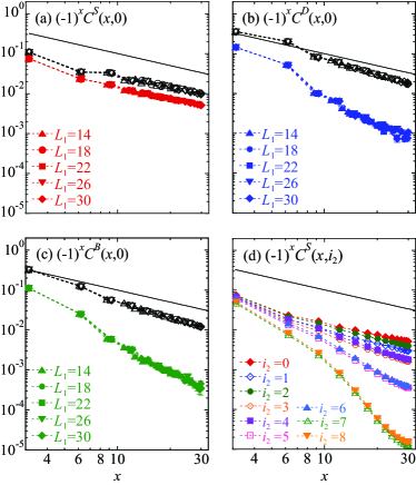
Figure 2: Real-space correlation functions of the model (7) for (a) spin, (b) dimer, and (c) bond at the domain wall of Z₂ KVBS (solid symbols). Here $L_{2}=17$ and $x=L_{1}{\rm sin}(\pi i_{1}/L_{1})$ is the conformal distance [24]. Open symbols indicates QMC results for the one-dimensional Hubbard model with $U/t=4$ and at half filling. (d) Real-space correlation functions of the model (7) for spin along the domain wall. Here, $L_{1}=30$ and $L_{2}=17$. Solid line denotes $(-1)^{x}x^{-1}$.

The field theory interpretation of the domain wall has consequences. It should be independent of the choice of the lattice discretization—provided that it does not break relevant symmetries such as translation along the domain wall—and the lattice constant should correspond to a high-energy scale. In Fig 2(d), we check that the domain wall extends over many lattice sites in the perpendicular direction. In particular, for the value of transverse field $h$ considered, the domain wall extends over several lattice spacings and the data are consistent with $C^{S}(x,i_{2})\sim e^{-|i_{2}|/\xi}x^{-1}$ where $\xi\sim 4$. Varying $1/h$ in the Z₂ KVBS will merely change the profile of the domain wall, thereby changing the length scale $\xi$ but not the properties of the spin-$1/2$ chain along the domain wall (see SM). If $1/h$ drops below $1/h_{c}$ into the AFM phase, spinons will bind and we expect long-range order to develop within the domain wall. Calculations confirming this point of view can be found in the SM.

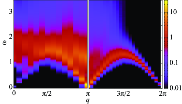
Figure 3: Dynamical spin structure factor $C^{S}(q,\omega)$ at the domain wall of the Z₂ KVBS (left panel). Here, $L_{1}=26$ and $L_{2}=17$. From the calculation of the single-particle gap on torus geometries (see the SM) we estimate the particle-hole continuum to lie above $\omega\simeq 1.5$. Right panel: dynamical spin structure factor for the Hubbard model on a 46-site chain at $U/t=4$ and at half filling.

Further evidence for an emergent spin-$1/2$ Heisenberg chain can be obtained from the dynamical spin structure factor at the domain wall of the Z₂ KVBS shown in the left panel of Fig. 3. The key feature of the spin-$1/2$ chain is that the low-lying excitations are well described by the two-spinon continuum revealed by the dynamical spin structure factor. In the thermodynamic limit, such excitations have a support in the wave vector, $q$, versus frequency, $\omega$, plane with lower and upper bounds given by $\omega_{\text{l}}(q)\sim\pi/2|\sin(q)|$ and $\omega_{\text{u}}(q)\sim\pi|\sin(q/2)|$, respectively. Experimental as well as theoretical calculations of the dynamical spin structure factor can be found in Ref. [25]. Figure 3 shows the results for the dynamical spin structure factor $C^{S}(q,\omega)$ at the domain wall of the Z₂ KVBS. In our QMC simulations, $C^{S}(q,\omega)$ was obtained via the analytic continuation of the imaginary-time-displaced spin correlation functions $C^{S}(q,\tau)=\langle\hat{\boldsymbol{S}}_{q}(\tau)\cdot\hat{\boldsymbol{S}}_{-q}(0)\rangle={L_{1}}^{-1}\sum_{i_{1}}e^{iqi_{1}}\langle\hat{\boldsymbol{S}}_{(i_{1},0)}(\tau)\cdot\hat{\boldsymbol{S}}_{\boldsymbol{0}}(0)\rangle$ at $i_{2}=0$. Below the particle-hole continuum, estimated to start at $\omega>1.5t$, our QMC results reproduce the well-known features of the two-spinon continuum [see the right panel of Fig. 3].

Summary and discussion.—We have shown how to probe topological terms in lattice realizations of field theories by pinning defects. The explicit example provided in this work is based on a model where the effective field theory has a $\theta$-term at $\theta=\pi$ in 2+1 dimensions with emergent SO(4) symmetry. In the lattice realization of this model, the SO(4) symmetry reduces to SO(3)$\times$ Z₂ and we consider a domain wall of the Z₂ field. The emergent SO(4) symmetry then suggests that the domain wall harbors a spin-$1/2$ chain. Our numerical results confirm this point of view.

The above argument holds for continuous transitions with emergent symmetries. There is an ongoing debate on the nature of the generic DQCP between AFM and VBS [26; 27; 28] (or quantum spin Hall (QSH) and s-wave superconducting (SSC) [29]) orders with emergent SO(5) symmetry [30]. Compelling evidence for a continuous transition as well as emergent SO(5) symmetry from finite-size calculations has been put forward. However the critical exponents stand at odds with the bootstrap bounds [31]. To resolve this apparent contradiction, one can conjecture [32; 33; 34] that an SO(5) conformal field theory indeed exists in spatial dimensions slightly greater than two that, however, collides with another fixed point and becomes complex upon tuning the dimension down to two. Proximity to fixed-point collision is at the origin of a very slow renormalization group flow and associated very long correlation lengths [35; 32]. In fact, recent simulations of the SO(5) non-linear sigma model with a WZW topological term support this point of view [36]. Very similar arguments can be applied to the present case where weakly first-order transitions were reported for similar symmetry classes [37; 38; 39]. Hence, a weakly first-order transition does not impair the notion that topological terms can play a dominant role at intermediate length scales.

Our approach can also be applied to other models. For the AFM-VBS transition, pinning a C₄ vortex on a system with open boundary conditions should result in a spinon that can be probed via the spin susceptibility. In the context of the QSH-SSC transition of Ref. [29] it is possible to pin a skyrmion of the O(3) QSH order parameter. Since topology states that the skyrmion carries charge 2e [5] this should result in a doping of the system.

Our observation may have some utility in three dimensions, where there are also pairs of ordered phases for which the disorder operators for one phase are charged under the symmetry broken by the other. A simple example involves a cubic-lattice AFM and a cubic-lattice VBS [40]. As in two dimensions, the skyrmions carry lattice-symmetry quantum numbers, and the defects of the VBS pattern (which are hedgehogs) carry spin. This can be encoded in a sigma model with a WZW term, now with softly-broken $\mathrm{SO}(6)\supset\mathrm{SO(3)}_{\mathrm{AFM}}\times\mathrm{SO(3)}_{\mathrm{VBS}}$ symmetry. However, in addition to the usual possibility of a first-order transition [41], a direct transition between these two phases can also be preempted by an intermediate disordered phase for the following reason: in contrast to two dimensions, compact abelian gauge theory with small amounts of charged matter (QED) has a (familiar) deconfined phase in three dimensions. But, as in the above discussion, the WZW term still has consequences within the ordered phases. For definiteness and similarity with our example above, consider breaking the cubic lattice symmetry down to $\mathrm{Z}_{2}\times\mathrm{Z}_{2}$, where the second $\mathrm{Z}_{2}$ represents reflections in $\hat{z}$, say. The associated sigma model then has $\mathrm{SO}(5)\supset\mathrm{SO}(3)_{\mathrm{AFM}}\times(\mathrm{Z}_{2}\times\mathrm{Z}_{2})_{\mathrm{VBS}}$ symmetry with a $\theta$-term at $\theta=\pi$. In analogy to the case considered here, the domain wall of the Z₂ part of the VBS order parameter transverse to the $\hat{z}$ direction will host an SO(4) non-linear sigma model at $\theta=\pi$, now in $2+1$ dimensions. This is a description of the deconfined critical point between AFM and KVBS orders in two dimensions. Along a domain wall of the VBS pattern, spin and VBS correlations are predicted to be long-ranged, with the same exponents.

Another possibility is to break the cubic lattice symmetry down to $\mathrm{C}_{4}\times\mathrm{Z}_{2}$, where again the $\mathrm{Z}_{2}$ represents reflections in $\hat{z}$. The associated sigma model then has $\mathrm{SO}(6)\supset\mathrm{SO}(3)_{\mathrm{AFM}}\times(\mathrm{SO}(2)\times\mathrm{Z}_{2})_{\mathrm{VBS}}$ symmetry with a WZW term. Now, the domain wall of the $\mathrm{Z}_{2}$ part of the VBS order parameter, transverse to the $\hat{z}$ direction, will host an $\mathrm{SO}(5)$ non-linear sigma model with a WZW term, now in $2+1$ dimensions. This construction could provide an alternative for the Landau-level projection formulation of this theory [42; 36]. This is a description of the DQCP between AFM and VBS.

I Supplemental Material

In this supplemental material we will first derive the domain wall action: a (1+1) dimensional SO(3) non-linear sigma model with $\theta$-term at $\theta=\pi$. Next we will review our auxiliary-field quantum Monte Carlo (AFQMC) simulations on the torus. They support the point of view that—on the accessible lattice sizes–our model indeed shows a continuous transition between an SO(3) antiferromagnet (AFM) and Z₂ KVBS with emergent SO(4) symmetry. We then provide more data on the profile of the domain wall and spin dynamics along the domain wall when tuning through the transition. Finally, we will show that AFQMC simulations of the one-dimensional repulsive Hubbard model at half filing reproduce the expected power-law decay of real-space spin, dimer, and bond correlation functions.

II Spin-1/2 chain pinned at the Z₂ domain wall: a field theoretic approach

In this section, we will detail the calculation that shows that starting from the $\theta$-term at $\theta=\pi$, a domain wall of $\mathrm{Z}_{2}$ KVBS nucleates a spin-$1/2$ chain. Our starting point is the field theory discussed in the main text:

$$S=\int dx^{2}d\tau\frac{1}{g}(\partial_{u}\hat{\boldsymbol{\phi}})^{2}+i\theta{\cal Q}~{}~{},~{}~{}\theta=\pi$$ (8)

with

$${\cal Q}=\frac{1}{12\pi^{2}}\int dx^{2}d\tau\epsilon_{i,j,k}\epsilon_{\alpha,\beta,\gamma,\delta}\hat{{\phi}}_{\alpha}\partial_{i}\hat{{\phi}}_{\beta}\partial_{j}\hat{{\phi}}_{\gamma}\partial_{k}\hat{{\phi}}_{\delta}.$$ (9)

Here, $\hat{\boldsymbol{\phi}}=\hat{\boldsymbol{\phi}}(\boldsymbol{x},\tau)$ defines a mapping between the $2+1$ dimensional Euclidean space-time to the unit sphere in four dimensions: $S^{3}$. For any smooth field configuration, ${\cal Q}$ counts the winding of the unit four-vector $\hat{\boldsymbol{\phi}}=\boldsymbol{\phi}/|\boldsymbol{\phi}|$ on the hypersphere $S^{3}$ and takes an integer value. The value of $\theta$ is thereby of great importance. One can start from the Wess-Zumino-Witten term that appears in a setting where the Dirac fermions couple symmetrically to a quintuplet of anti-commuting mass terms and set one mass to zero. A calculation will then lead to the aforementioned $\theta$-term at $\theta=\pi$ [3]. Here, our aim is to consider a domain-wall configuration. For the calculation to be well defined, we have to make sure that the field configuration $\hat{\boldsymbol{\phi}}(\boldsymbol{x},\tau)$ has no singularities. To achieve this goal, it is useful to include the point at infinity in Euclidean space, so that the base space is topologically a three-sphere. We can specify coordinates by embedding the three-sphere into $\mathbb{R}^{4}$ Euclidean space by

$$x_{1}=\cos(\varphi_{1})$$

$$x_{2}=\sin(\varphi_{1})\cos(\varphi_{2})$$

$$x_{3}=\sin(\varphi_{1})\sin(\varphi_{2})\cos(\varphi_{3})$$

$$x_{4}=\sin(\varphi_{1})\sin(\varphi_{2})\sin(\varphi_{3})$$ (10)

where $\varphi_{1}\in[0,\pi]$, $\varphi_{2}\in[0,\pi]$, and $\varphi_{3}\in[0,2\pi]$. Since the topological term is independent of the choice of the metric we obtain with this parameterization:

$${\cal Q}=\frac{1}{12\pi^{2}} \int_{0}^{\pi}d\varphi_{1}\int_{0}^{\pi}d\varphi_{2}\int_{0}^{2\pi}d\varphi_{3}$$ (11)

$$\epsilon_{i,j,k}\epsilon_{\alpha,\beta,\gamma,\delta}{\hat{\phi}}_{\alpha}\partial_{i}{\hat{\phi}}_{\beta}\partial_{j}{\hat{\phi}}_{\gamma}\partial_{k}{\hat{\phi}}_{\delta}$$

with $\partial_{i}=\frac{\partial}{\partial\varphi_{i}}$. With this compactification of $\mathbb{R}^{3}$ we can define a smooth domain-wall configuration as:

$${\hat{\phi}}_{4}=\cos(f(\varphi_{1}))$$

$${\hat{\phi}}_{3}=\sin(f(\varphi_{1}))n_{3}$$

$${\hat{\phi}}_{2}=\sin(f(\varphi_{1}))n_{2}$$

$${\hat{\phi}}_{1}=\sin(f(\varphi_{1}))n_{1}$$ (12)

Here $\boldsymbol{n}(\varphi_{2},\varphi_{3})=\left(n_{1},n_{2},n_{3}\right)$. From $|\hat{\boldsymbol{\phi}}|=1$ follows that $|\boldsymbol{n}|=1$. $\varphi_{2}$ and $\varphi_{3}$ define a point on the unit sphere in three dimensions, $S^{2}$, that is isomorphic to $\mathbb{R}^{2}$. Hence, $\boldsymbol{n}$ defines a mapping from $\mathbb{R}^{2}$ to the unit sphere in $\mathbb{R}^{3}$.

We can now return to $\hat{\boldsymbol{{\phi}}}$. The function $f(\varphi_{1})$ defines a generic domain wall and is required to satisfy the following properties. $f(0)=0$, $f(\pi)=\pi$ and $f(\varphi_{1})$ is a one-to-one mapping from $\left[0,\pi\right]$ to $\left[0,\pi\right]$. At infinity in $\mathbb{R}^{3}$, corresponding to $\varphi_{1}=0$, $\hat{\boldsymbol{{\phi}}}=(0,0,0,1)$ and at the origin, $\varphi_{1}=\pi$, $\hat{\boldsymbol{{\phi}}}=(0,0,0,-1)$. The pinning of $\hat{\boldsymbol{{\phi}}}$ at the origin and at infinity defines a Z₂ domain wall in the fourth component of the field. This choice of the field $\hat{\boldsymbol{\phi}}$ explicitly breaks SO(4) symmetry down to SO(3) corresponding to rotations of the $\boldsymbol{n}$ vector.

For the domain-wall field configuration of Eq. II, we can evaluate the $\theta$-term by explicitly carrying out the integration over $\varphi_{1}$. Since $f(\varphi_{1})$ is a one-to-one mapping and ${\cal Q}$ is a topological quantity, the value of ${\cal Q}$ for the domain wall field of Eq. II is identical to the deformed domain wall:

$$\hat{\phi}_{4}=\cos(\varphi_{1})$$

$$\hat{\phi}_{3}=\sin(\varphi_{1})n_{3}$$

$$\hat{\phi}_{2}=\sin(\varphi_{1})n_{2}$$

$$\hat{\phi}_{1}=\sin(\varphi_{1})n_{1}.$$ (13)

Inserting this result in ${\cal Q}$ and evaluating the integral over $\varphi_{1}$ gives

$${\cal Q}_{\text{DW}}=\frac{1}{4\pi}\int_{0}^{\pi}d\varphi_{2}\int_{0}^{2\pi}d\,\varphi_{3}\,\boldsymbol{n}\cdot\partial_{\varphi_{2}}\boldsymbol{n}\times\partial_{\varphi_{3}}\boldsymbol{n}.$$ (14)

In summary, the domain-wall action reads

$$S_{DW}=\int dxd\tau\frac{1}{g}(\partial_{u}\hat{\boldsymbol{n}})^{2}+i\pi{\cal Q}_{\text{DW}},$$ (15)

which corresponds to the coherent spin state path integral of the spin-$1/2$ chain [14; 15].

III Continuous AFM-Z₂ KVBS transition with emergent SO(4) symmetry

As mentioned in the main text, our calculations in [6] were carried out on the honeycomb lattice. Here, we map out the bulk phase diagram on a torus geometry for the $\pi$-flux lattice and show that the model has a similar phase diagram.

We consider a model of Dirac fermions in $2+1$ dimensions with Hamiltonian $\hat{H}=\hat{H}_{\text{f}}+\hat{H}_{\text{s}}+\hat{H}_{\text{fs}}$ (see Fig.1(b) of the main text):

$$\hat{H}_{\text{f}} =\sum_{\langle\boldsymbol{i}\boldsymbol{j}\rangle,\sigma}t_{\boldsymbol{i}\boldsymbol{j}}\hat{c}_{\boldsymbol{i}\sigma}^{\dagger}\hat{c}_{\boldsymbol{j}\sigma}+U\sum_{\boldsymbol{i}}(\hat{n}_{\boldsymbol{i}\uparrow}-\mbox{$\frac{1}{2}$})(\hat{n}_{\boldsymbol{i}\downarrow}-\mbox{$\frac{1}{2}$}),$$

$$\hat{H}_{\text{s}} =J\sum_{\langle\boldsymbol{i}\boldsymbol{j},\boldsymbol{k}\boldsymbol{l}\rangle}\hat{s}_{\boldsymbol{i}\boldsymbol{j}}^{z}\hat{s}_{\boldsymbol{k}\boldsymbol{l}}^{z}-h\sum_{\langle\boldsymbol{i}\boldsymbol{j}\rangle}\hat{s}_{\boldsymbol{i}\boldsymbol{j}}^{x},$$

$$\hat{H}_{\text{fs}} =\sum_{\langle\boldsymbol{i}\boldsymbol{j}\rangle,\sigma}t_{\boldsymbol{i}\boldsymbol{j}}\xi_{\boldsymbol{i}\boldsymbol{j}}\hat{s}_{\boldsymbol{i}\boldsymbol{j}}^{z}\hat{c}_{\boldsymbol{i}\sigma}^{\dagger}\hat{c}_{\boldsymbol{j}\sigma}.$$ (16)

Here $\hat{H}_{\text{f}}$ corresponds to the half-filled Hubbard model on the $\pi$-flux square lattice. $\hat{c}_{\boldsymbol{i}\sigma}(\hat{c}_{\boldsymbol{i}\sigma}^{\dagger})$ is the fermionic annihilation (creation) operator at site $\boldsymbol{i}$ with spin $\sigma=\uparrow,\downarrow$, and $\hat{n}_{\boldsymbol{i}\sigma}\equiv\hat{c}_{\boldsymbol{i}\sigma}^{\dagger}\hat{c}_{\boldsymbol{i}\sigma}$. $\hat{H}_{\text{s}}$ is a ferromagnetic, transverse-field Ising model where the Ising spins—described by the Pauli spin operators $\hat{s}_{\boldsymbol{i},\boldsymbol{j}}^{\alpha}(\alpha=x,y,z)$—live on the bonds connecting fermionic sites $\boldsymbol{i}$ and $\boldsymbol{j}$. $J$ is the ferromagnetic nearest-neighbor interaction and $h$ the transverse field. $\hat{H}_{\text{fs}}$ accounts for the coupling ($\xi_{\boldsymbol{i}\boldsymbol{j}}=\pm\xi$) between Dirac fermions and Ising spins. Our model Hamiltonian $\hat{H}$ has an SU(2) spin symmetry as well as a Z₂ symmetry corresponding to invariance under the combined operation of inversion and $\hat{s}_{\boldsymbol{i}\boldsymbol{j}}^{z}\to-\hat{s}_{\boldsymbol{i}\boldsymbol{j}}^{z}$. Under inversion $\hat{H}_{\text{fs}}\to-\hat{H}_{\text{fs}}$, so that the energy does not depend on the sign of $\xi$ and the two possible Kekulé patterns related by $\xi\to-\xi$ are degenerate. The Hubbard interaction and the fermion-spin coupling have the potential to dynamically generate SO(3) AFM order and Z₂ KVBS order (ferromagnetic order of the Ising spins), respectively.

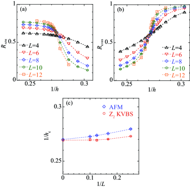
Figure 4: Correlation ratios for (a) AFM and (b) $\mathrm{Z}_{2}$ KVBS states at $U=7$. (c) Extrapolation of crossing points of correlation ratios for $L$ and $L+2$ gives the critical value $\left(h_{c}^{\text{AFM}}\right)^{-1}\approx\left(h_{c}^{\text{KVBS}}\right)^{-1}\approx 0.270$.

We used the ALF (Algorithms for Lattice Fermions) implementation [16] of the well-established finite-temperature auxiliary-field QMC method [17; 18]. Simulations of our model are free of the negative sign problem. To see this, one can first carry out a partial particle-hole canonical transformation: $\hat{c}_{\boldsymbol{i},\uparrow}\rightarrow e^{i\boldsymbol{Q}\cdot\boldsymbol{i}}\hat{c}^{\dagger}_{\boldsymbol{i},\uparrow}$ and $\hat{c}_{\boldsymbol{i},\downarrow}\rightarrow\hat{c}_{\boldsymbol{i},\downarrow}$ with $\boldsymbol{Q}=(\pi,\pi)/a$. This changes the sign of the Hubbard interaction from positive to negative. One can the use time reversal symmetry to show that the eigenvalues of the Fermion determinant come in complex conjugate pairs [43]. We simulated lattices with $L\times L$ unit cells (each containing four Dirac fermions and four Ising spins) and periodic boundary conditions. Henceforth, we use $t=1$ as the energy unit, set $J=-1$, $\xi=0.5$, and $U=7$. All the data are for the Trotter discretization $\Delta\tau=0.1$. In the considered parameter range, an inverse temperature $\beta=30$ was sufficient to obtain results representative of the ground state.

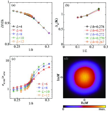
Figure 5: (a) Free-energy derivative and (b) single-particle gap at the Dirac point $\boldsymbol{q}=\boldsymbol{K}$. (c) Ratio of the standard deviations of the AFM and Z₂ KVBS order parameters. (d) Joint probability distribution of the two order parameters at the critical point for $L=8$. Here, $U=7$ and $\beta=30$.

The dashed line in Fig. 1 (a) of the main text indicates the scan of the phase diagram obtained by tuning $h$ at a fixed $U=7$. Along this line we observe two insulating phases corresponding to the SO(3) AFM and the Z₂ KVBS.

To map out the phase diagram we compute equal-time correlation functions of fermion spin $\hat{\boldsymbol{S}}_{\boldsymbol{i}}=\sum_{\sigma\sigma^{\prime}}\hat{c}_{\boldsymbol{i}\sigma}^{\dagger}\boldsymbol{\sigma}_{\sigma\sigma^{\prime}}\hat{c}_{\boldsymbol{i}\sigma^{\prime}}$, fermion bond $\hat{B}_{\boldsymbol{i}\boldsymbol{j}}=\sum_{\sigma}t_{\boldsymbol{i}\boldsymbol{j}}(\hat{c}_{\boldsymbol{i}\sigma}^{\dagger}\hat{c}_{\boldsymbol{j}\sigma}+\hat{c}_{\boldsymbol{j}\sigma}^{\dagger}\hat{c}_{\boldsymbol{i}\sigma})$, and Ising spin $\hat{s}_{\boldsymbol{i}\boldsymbol{j}}^{z}$. Due to the larger unit cell, these correlation functions are $4\times 4$ matrices of the form $C^{O}_{\boldsymbol{R}\gamma,\boldsymbol{R}^{\prime}\delta}=\langle(\hat{{O}}_{\boldsymbol{R}\gamma}-\langle\hat{{O}}_{\boldsymbol{R}\gamma}\rangle)\cdot(\hat{{O}}_{\boldsymbol{R}^{\prime}\delta}-\langle\hat{{O}}_{\boldsymbol{R}^{\prime}\delta}\rangle)\rangle$ ($\hat{O}=\hat{\boldsymbol{S}},\hat{B},\hat{s}$) where $\boldsymbol{R},\boldsymbol{R}^{\prime}$ labels the unit cell and $\gamma,\delta$ the orbitals. After diagonalizing the corresponding structure factors

$$C^{O}_{\gamma\delta}(\boldsymbol{q})=\frac{1}{L^{2}}\sum_{\boldsymbol{R}\boldsymbol{R}^{\prime}}C^{O}_{\boldsymbol{R}\gamma,\boldsymbol{R}^{\prime}\delta}e^{i{\boldsymbol{q}}\cdot(\boldsymbol{R}-\boldsymbol{R}^{\prime})},$$ (17)

we calculated the renormalisation-group invariant correlation ratio [44; 45]

$$R_{O}=1-\frac{\lambda_{1}({\boldsymbol{q}}_{0}+\delta{\boldsymbol{q}})}{\lambda_{1}({\boldsymbol{q}}_{0})}$$ (18)

using the largest eigenvalue $\lambda_{1}({\boldsymbol{q}})$; ${\boldsymbol{q}}_{0}$ is the ordering wave vector, ${\boldsymbol{q}}_{0}+\delta{\boldsymbol{q}}$ a neighboring wave vector. By definition, $R_{O}\to 1$ for $L\to\infty$ in the corresponding ordered state, whereas $R_{O}\to 0$ in the disordered state. At the critical point, $R_{O}$ is scale-invariant for sufficiently large $L$ so that results for different system sizes cross. Figures 4 (a) and (b) show the results. Based on the assumption of a dynamical critical exponent $z=1$ [46] we set $L=\beta$ to carry out the finite-size scaling. The onset of the AFM is detected from the crossing of $R_{\text{AFM}}\equiv R_{S}$ [Fig. 4(a)], whereas the onset of Kekulé order can be detected either from $R_{\text{KVBS}}\equiv R_{s}$ [Fig. 4(b)] or from $R_{B}$. The finite-size scaling of the crossing points yields a single critical point of $h_{c}^{-1}\approx 0.270$ shown in Fig. 4 (c), pointing to a direct phase transition between AFM and Z₂ KVBS.

Figure 5 (a) plots the free-energy derivative

$$\frac{\partial F}{\partial h}=\frac{1}{4L^{2}}\left<\sum_{\langle\boldsymbol{i}\boldsymbol{j}\rangle}\hat{s}_{\boldsymbol{i}\boldsymbol{j}}^{x}\right>.$$ (19)

The absence of a discontinuity in this quantity favors a continuous transition.

For the derivation of a low-energy effective field theory is important to confirm that the single particle gap remains finite across the transition. We measured the imaginary-time displaced Green’s function $G({\boldsymbol{q}},\tau)$ and obtained the single-particle gap $\Delta_{\text{sp}}({\boldsymbol{q}})$ from

$$G({\boldsymbol{q}},\tau)\propto\exp(-\tau\Delta_{\text{sp}}({\boldsymbol{q}}))$$ (20)

at large imaginary time $\tau$. We found that the single-particle gap at the Dirac point, shown in Fig. 5(b), remains clearly nonzero.

To verify whether the critical point has an emergent SO(4) symmetry, we measured the standard deviations $\sigma_{O}=\sqrt{\langle\hat{O}^{2}\rangle-\langle\hat{O}\rangle^{2}}$ of the AFM ($\sigma_{\text{AFM}}\equiv\sigma_{S}$) and Z₂ KVBS ($\sigma_{\text{KVBS}}\equiv\sigma_{s})$ order parameters. These quantities are in general independent but become locked together and can be combined into a four-component order parameter if an SO(4) symmetry—unifying the two order parameters—emerges at the critical point. In this case, the ratio $\sigma_{\rm KVBS}/\sigma_{\rm AFM}$ will become universal at the critical point. This is confirmed by the result in Fig. 5(c). Moreover, the emergent SO(4) symmetry can also be confirmed in the joint probability distribution of the two order parameters determined from QMC snapshots,

$$\boldsymbol{M}=\sigma_{\text{AFM}}e^{i0}+\sigma_{\text{KVBS}}e^{\frac{i\pi}{2}}.$$ (21)

If the SO(4) symmetry emerges at the critical point, the quantity $\boldsymbol{M}$ (after normalization of each order parameter) should reveal a circular distribution, as confirmed at the critical point by Fig. 5(d).

IV Spin dynamics around the Z₂ domain wall with varying $1/h$

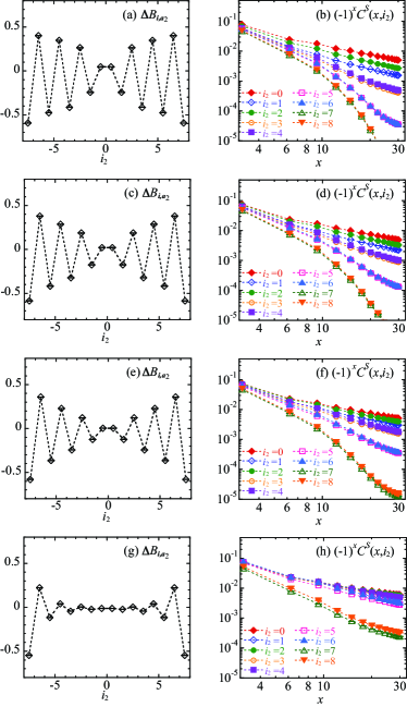
Figure 6: Real-space bond energy change $\Delta\hat{B}_{\boldsymbol{i},\boldsymbol{a}_{2}}$ at $\boldsymbol{i}=(i_{1}=0,i_{2})$ (left panel) and real-space spin-spin correlation functions along the domain wall of $\mathrm{Z}_{2}$ KVBS $C^{S}(x,i_{2})$ (right panel) for $L_{1}=30$ and $L_{2}=17$. Here $x=L_{1}{\rm sin}(\pi i_{1}/L_{1})$ is the conformal distance. Parameters used are $1/h=0.333$ [(a) and (b) in the $\mathrm{Z}_{2}$ KVBS phase], $1/h=0.299$ [(c) and (d) in the $\mathrm{Z}_{2}$ KVBS phase], $1/h=0.275$ [(e) and (f) in the $\mathrm{Z}_{2}$ KVBS phase close to the critical point], and $1/h=0.033$ [(g) and (h) in the AFM phase]. Here, $U=7$ and $\beta=30$.

In the main text we set $1/h=0.275$ that places us in the $\mathrm{Z}_{2}$ KVBS phase close to the critical point. Here we vary $1/h$ across the transition and investigate the fate of the domain wall. In Fig. 6 we map out the profile of the domain wall by considering $\Delta\hat{B}_{\boldsymbol{i},\boldsymbol{a}_{2}}$ across the domain wall (left panels) the spin correlations along the domain wall (right panels). These quantities are defined in the main text.

The profile of the domain wall in the KVBS phase is expected to be inversely proportional to the stiffness. Indeed the QMC results shown in Figs. 6 (a)-(f) support that upon moving away from the critical point deep into the $\mathrm{Z}_{2}$ KVBS phase the domain wall becomes more pronounced. Accordingly the width around the domain wall where one observes $1/r$ decay of the spin-spin correlations reduces.

In the AFM phase there is no scale that confines the width of the domain wall other than the width of the lattice $L_{2}$. We equally expect the spin-spin correlations to show long range order. In Fig. 6 (g)-(h) we consider a very large value of $h=30$. As apparent from Fig. 6 (g) the profile of the domain wall is very flat around the center of the cylinder. The spin correlations show a slight upturn but remarkably do not provide clear evidence of long range order. We can understand this in the following way. The AFM state originates from the binding of spinons and this will occur on a given length scale. If $L_{2}$ is comparable to this length scale, then long range order will be hard to detect. We hence conjecture that as $L_{2}$ grows spin-spin correlations will develop clear signs of ordering.

V One dimensional Hubbard model at half filling

In this section, we present QMC results of the one-dimensional repulsive Hubbard model at half filling. The Hamiltonian is

$$\hat{H}=t\sum_{i,\sigma}\hat{c}_{i\sigma}^{\dagger}\hat{c}_{i+1\sigma}+H.c.+U\sum_{i}(\hat{n}_{i\uparrow}-\mbox{$\frac{1}{2}$})(\hat{n}_{i\downarrow}-\mbox{$\frac{1}{2}$}),$$

(22)

where $t$ is the nearest-neighbor hopping amplitude and $U$ is the Hubbard repulsion. $\hat{c}_{i\sigma}(\hat{c}_{i\sigma}^{\dagger})$ is the fermionic annihilation (creation) operator at site $i$ with spin $\sigma=\uparrow,\downarrow$, and $\hat{n}_{i\sigma}\equiv\hat{c}_{i\sigma}^{\dagger}\hat{c}_{i\sigma}$. For the numerical simulations we used the ALF (Algorithms for Lattice Fermions) implementation [16] of the well-established auxiliary-field quantum Monte Carlo (AFQMC) method [17; 18]. We carried out ground-state simulations with the projective AFQMC algorithm, which is based on the equation

$$\langle\hat{O}\rangle_{\hat{H}}=\lim_{\Theta\to\infty}\frac{\langle\psi_{T}|e^{-\frac{\Theta}{2}\hat{H}}\hat{O}e^{-\frac{\Theta}{2}\hat{H}}|\psi_{T}\rangle}{\langle\psi_{T}|e^{-{\Theta}\hat{H}}|\psi_{T}\rangle},$$ (23)

where $\Theta$ is a projection parameter. The trial wave function $|\psi_{T}\rangle$ is chosen to correspond to the ground state of the noninteracting Hamiltonian. We simulated lattice sizes ranging from $L=14$ to $510$ with periodic boundary conditions. Henceforth, we use $t=1$ as the energy unit and set $U=4$. All the data were obtained for $\Theta=30$ (and Trotter discretization $\Delta\tau=0.1$), sufficient to obtain results representative of the ground state for the parameters considered.

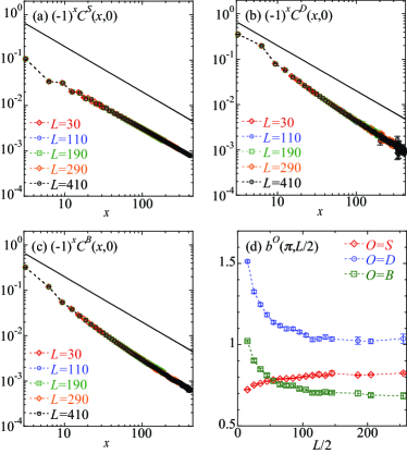
Figure 7: Real-space correlation functions of the one-dimensional repulsive Hubbard model at half filling for (a) spin, (b) dimer, and (c) bond. Here $x=L{\rm sin}(\pi r/L)$ is the conformal distance. Solid line correspond to $(-1)^{x}x^{-1}$. (d) $b^{S}(q,L/2)$, $b^{D}(q,L/2)$, and $b^{B}(q,L/2)$ at $q=\pi$ (see text).

We measured real-space correlation functions of spin $\hat{{\boldsymbol{S}}}_{i}=\sum_{\sigma\sigma^{\prime}}\hat{c}_{i\sigma}^{\dagger}\boldsymbol{\sigma}_{\sigma\sigma^{\prime}}\hat{c}_{i\sigma^{\prime}}$, dimer $\hat{{\boldsymbol{D}}}_{i}=\hat{{\boldsymbol{S}}}_{i}\cdot\hat{{\boldsymbol{S}}}_{i+1}$, and bond $\hat{B}_{i}=\sum_{\sigma}(\hat{c}_{i\sigma}^{\dagger}\hat{c}_{i+1\sigma}+\hat{c}_{i+1\sigma}^{\dagger}\hat{c}_{i\sigma})$,

$$C^{S}(r) =\langle\hat{\boldsymbol{S}}_{r}\cdot\hat{\boldsymbol{S}}_{0}\rangle,$$ (24)

$$C^{D}(r) =\langle(\hat{\boldsymbol{D}}_{r}-\langle\hat{\boldsymbol{D}}_{r}\rangle)\cdot(\hat{\boldsymbol{D}}_{0}-\langle\hat{\boldsymbol{D}}_{0}\rangle)\rangle,$$ (25)

$$C^{B}(r) =\langle(\hat{B}_{r}-\langle\hat{B}_{r}\rangle)\cdot(\hat{B}_{0}-\langle\hat{B}_{0}\rangle)\rangle.$$ (26)

The ground state of the SU(2) symmetric isotropic spin-$1/2$ Heisenberg chain is conformally invariant. Spin correlation functions scale as $\sim(-1)^{r}(\ln{r})^{1/2}r^{-1}$, with multiplicative logarithmic corrections [21; 22; 23]. Owing to emergent SO(4) symmetry [19; 20], dimer correlation functions exhibit the same exponent but different logarithmic corrections; they decay as $\sim(-1)^{r}(\ln{r})^{-3/2}r^{-1}$ [23]. Here we consider the half-filled Hubbard Hamiltonian that maps onto the Heisenberg model.

Figures 7(a) and (b) show QMC results for spin and dimer correlation functions, which indicate that the correlation functions both yield consistent power-law decay at large conformal distances, $x=L{\rm sin}(\pi r/L)$. The bond correlations have the same symmetry properties as the dimer correlations so that we expect the same power-law decay. This can be confirmed by the QMC results shown in Fig. 7 (c). The exponent of the power-law decay can be detected using the quantity [47]

$$b^{O}(q,L/2) \equiv C^{O}(q)$$ (27)

$$-C^{O}(q+2\pi/L)-C^{O}(q-2\pi/L),$$

where $C^{O}(q)$ corresponds to the static structure factor of the local observable $O$. One can show that the real space correlations at distance $C^{O}(L/2)=\frac{1}{4L}\sum_{q}e^{iqL/2}b^{O}(q,L/2)$. This formula singles out the wave numbers where the static structure factor shows non-analytical behavior. In our case, this is the case at $q=\pi$ so that

$$C^{O}(L/2)\propto\frac{1}{L}e^{i\pi L/2}b^{O}(q=\pi,L/2).$$ (28)

Assuming that $C^{O}(L/2)\propto\alpha e^{i\pi L/2}(L/2)^{-K}(\ln(L/2))^{\gamma}$ then

$$\ln(b^{O}(\pi,L/2))\propto\alpha^{\prime}+(-K+1)\ln(L/2)+\gamma\ln(\ln(L/2)).$$ (29)

Figure 7(d) plots this quantity for spin, dimer, and bond correlations as a function of $L/2$. All three quantities are nearly constant for large values of $L/2$, thus confirming $K=1$. Differences in $b^{D}(\pi,L/2)$ and $b^{S}(\pi,L/2)$ arise from the third term on the right-hand side of Eq. (29), reflecting the different logarithmic corrections. Since bond correlations have the same symmetry properties as the dimer correlations, the logarithmic corrections are expected to be consistent.