Non-dispersing wave packets in lattice Floquet systems

Abstract

We show that in a one-dimensional translationally invariant tight binding chain, non-dispersing wave packets can in general be realized as Floquet eigenstates—or linear combinations thereof—using a spatially inhomogeneous drive, which can be as simple as modulation on a single site. The recurrence time of these wave packets (their “round trip” time) locks in at rational ratios $sT/r$ of the driving period $T$, where $s,r$ are co-prime integers. Wave packets of different $s/r$ can co-exist under the same drive, yet travel at different speeds. They retain their spatial compactness either infinitely ($s/r=1$) or over long time ($s/r\neq 1$). Discrete time translation symmetry is manifestly broken for $s\neq 1$, reminiscent of integer and fractional Floquet time crystals. We further demonstrate how to reverse-engineer a drive protocol to reproduce a target Floquet micromotion, such as the free propagation of a wave packet, as if coming from a strictly linear energy spectrum. The variety of control schemes open up a new avenue for Floquet engineering in quantum information sciences.

Introduction

It is well known that under a time-independent Hamiltonian, quantum wave packets typically spread out due to the presence of dispersion Messiah (1964). Since the birth of quantum mechanics, the stark contrast between the elusiveness of localized quantum entities and the stability of their classical counterparts has motivated physicists to explore ways to understand and even this disparity Schrödinger (2003); Nauenberg (2000); Buchleitner et al. (2002); Berry and Balazs (1979). Besides conceptual interest, such dynamically stable compact entities would hold technological utility in quantum information processing and computing platforms, since most control technologies are local in nature.

There are two known strategies for stabilization of non-dispersing wave packets. The first one relies on introducing some form of nonlinearity into the wave equation. For example, non-linear Schrödinger or Gross-Pitaevskii equations are known to host soliton solutions Knight and Miller (1992); Kivshar and Malomed (1989). The second one utilizes time-periodic Hamiltonian in the conventional linear Schrödinger equation, where recurring wave packets have been achieved with the help of Floquet engineering Buchleitner and Delande (1995); Holthaus (1995); Buchleitner et al. (2002); Maeda and Gallagher (2004); Kalinski et al. (2005); Vela-Arevalo and Fox (2005); Sacha (2015); Goussev et al. (2018). There, periodic driving serves to periodically reshape the wavepacket, curbing the irreversible dispersive spread characteristic of undriven systems. For example, this approach was applied in the context of microwave-driven Rydberg atoms Buchleitner et al. (2002); Maeda and Gallagher (2004); Dunning et al. (2009) to show that some Floquet eigenstates correspond to wave packets following classical Kepler orbits. While the shape of these wave packets is time-dependent, they refocus almost perfectly after integer number of drive periods. Intra-period, however, the packets would shrink or expand, in accordance with their (time-dependent) semiclassical velocity.

Floquet engineering is a very effective method to stabilize wave packets by means of a periodic drive, which does not need to be strong. However, up to now it has only been applied to systems that explicitly break spatial translation symmetry, such as electrons in ionic potential, or atomic condensates in gravitational field. Here the translation symmetry can be either continuous (for continuous systems) or discrete (for lattice systems). In this work, we generalize the Floquet engineering approach to create nondispersive wave packets in extended systems that do not break translation symmetry in the bulk when undriven. Examples include photons in extended microwave resonators, or particles (atoms, electrons) confined to a linear or circular resonators or chains of coupled resonators Suleymanzade et al. (2020); Ren et al. (2019); Kuzmin et al. (2019). Surprisingly, we discover that spatially localized driving is sufficient to generate compact dispersionless wave packets that are Floquet eigenstates. A traveling wave packet on such a device could conceivably serve as a “bus”, over which quantum information or a particle can be shuttled across the entire chain.

As a paradigmatic model we study a homogeneous tight binding chain. Depending on the number of sites and energy, it can implement either parabolic dispersion or approximate linear dispersion. The dispersion slope determines the group velocity, $v_{g}$, which, in combination with the system length, determines the wave packet’s recurrence time $T_{\text{rec}}$ (i.e., the time a wave packet takes to traverse one round trip of the system). This recurrence time is in general a function of energy.

A Floquet drive is defined by its period $T$, and its spatial and temporal profiles. We will see that $T$ singles out a series of spectral segments of the undriven system that are most susceptible to the formation of wave packets, as organized by their recurrence time $T_{\text{rec}}=\frac{s}{r}T$, where $s$ and $r$ are co-prime integers. The combination of the drive’s spatial and temporal profiles then imposes selection rules that determine which wave packets actualize, as well as their properties such as spatial compactness. When $s>1$, the Floquet wave packets manifestly break the discrete time-translation symmetry of the drive; we will discuss the connection to time crystal physics Wilczek (2012); Bruno (2013); Watanabe and Oshikawa (2015); Sacha (2015); Else et al. (2016); Khemani et al. (2016); Sacha and Zakrzewski (2017); Zhang et al. (2017). As long as these general rules are satisfied, the formation of wave packets is robust with respect to details such as the overall drive strength, the introduction of spatial or temporal randomness, etc. This flexibility also opens up the ability to fine-tune drive protocols for specific applications. As a proof of principle, we will demonstrate how to design a drive that reproduces a particular target Floquet micromotion.

Floquet wave packets at the primary resonance

To build intuition, we first discuss the emergence of Floquet wave packets at the primary resonance, that is those with a round trip time equal to the drive period, $T_{\text{rec}}=T$. Consider a time-periodic Hamiltonian $\hat{H}(t+T)=\hat{H}(t)$,

$$\hat{H}(t)=\hat{H}_{0}+\hat{V}(t)\ ,\ \hat{V}(t)=\sum_{a}g_{a}\hat{V}^{(a)}e^{ia\Omega t}\ ,$$ (1)

where $\hat{H}_{0}$ is the undriven tight-binding Hamiltonian, assumed to be spatially homogeneous, $\hat{V}^{(a)}$ encodes spatial dependence of the drive at frequency $a\Omega$, with relative strength $g_{a}$, and $\Omega=2\pi/T$ is the fundamental frequency. After one drive period, a Floquet eigenstate $|\psi\rangle$ returns to itself with an additional phase (quasienergy), $\hat{U}_{T}|\psi\rangle=e^{-i\theta}|\psi\rangle$, where $\hat{U}_{t}=\mathcal{T}\exp\left[-i\int_{0}^{t}dt^{\prime}\hat{H}(t^{\prime})\right]$ is the time evolution operator. This state can be lifted to a time-periodic trajectory in Hilbert space, i.e., a Floquet micromotion, $|\psi(t)\rangle=|\psi(t+T)\rangle=e^{+i\frac{\theta}{T}t}\hat{U}_{t}|\psi\rangle$, which satisfies the Floquet-Schrödinger equation,

$$\left[\hat{H}(t)-i\partial_{t}\right]|\psi(t)\rangle=\frac{\theta}{T}|\psi(t)\rangle\ .$$ (2)

Note that shifting $\theta\rightarrow\theta+2\pi a\ (a\in\mathbb{Z})$ leads to gauge equivalent micromotions $|\psi(t)\rangle\rightarrow|\psi(t)\rangle e^{ia\Omega t}$ of the same physical time evolution.

In the undriven limit, Floquet eigenstates are simply the energy eigenstates $|\varepsilon_{k}\rangle$ of $\hat{H}_{0}$ with integer label $k$. At weak drive, thus, most Floquet eigenstates are close to an undriven state and remain spatially extended. However, if the drive frequency $\Omega=2\pi/T$ is close to the level spacing $\Delta$ somewhere in the spectrum of $\hat{H}_{0}$, then the drive can efficiently couple several nearby unperturbed eigenstates. To describe this, one can expand a generic dispersion relation around some $k_{*}$ (not necessarily an integer), such that

$$\varepsilon_{k}=\varepsilon_{{*}}+(k-k_{*})\Omega+\frac{u}{T}(k-k_{*})^{2}+\cdots\ ,\ k\in\mathbb{Z}\ ,$$ (3)

and consider a micromotion ansatz

$$|\psi(t)\rangle=\sum_{k}f_{k}|\varepsilon_{k}\rangle e^{-ik\Omega t}\ .$$ (4)

Note that $|\varepsilon_{k}\rangle e^{-ik\Omega t}$ are Floquet micromotions in the undriven limit, and the gauge ($a=k$) is chosen so that near resonance, the corresponding quasienergies, $\theta_{k}^{(0)}=\varepsilon_{k}T-2\pi k$, are nearly degenerate (in the scale of $\Omega T=2\pi$), hence Eq. 4 is akin to degenerate perturbation solutions. For consistency, the range of the $k$ summation should be constrained such that $\{\theta_{k}^{(0)}\}$ are roughly within a single Floquet zone.

We assume positive $u$ and $\partial_{k}\varepsilon_{k}$ in Eq. 3; the case with one or both of them negative can be similarly handled. The coefficients $\{f_{k}\}$ are determined as the “degenerate perturbation” solutions of the Floquet-Schrödinger operator in the Hilbert space of the ansatz (Eq. 4),

$$\sum_{k^{\prime}}\left[u(k-k_{*})^{2}\delta_{k\,k^{\prime}}+g_{k^{\prime}-k}V_{kk^{\prime}}\right]f_{k^{\prime}}=(\theta-\theta_{*})f_{k}\ ,$$ (5)

where $V_{kk^{\prime}}=\langle\varepsilon_{k}|\hat{V}^{(k^{\prime}-k)}|\varepsilon_{k^{\prime}}\rangle T$ and $\theta_{*}=\varepsilon_{*}T-2\pi k_{*}$. Eq. 5 maps our problem to an effective one-dimensional “lattice” with quadratic “on-site potential” $u(k-k_{*})^{2}$ and “hopping” $g_{k^{\prime}-k}V_{kk^{\prime}}$. One thus expects on general grounds that its eigenstates will mix different $k$ “sites.” Translating back to the original problem, the Floquet micromotion $|\psi(t)\rangle$ is thus a linear superposition of momentum states $|\varepsilon_{k}\rangle$ with time-independent weights $|f_{k}|^{2}$, and is therefore a wave packet in coordinate space.

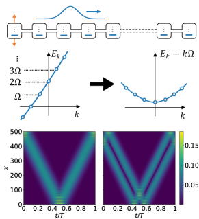
Figure 1: Top: schematic of coupled resonators. Temporal modulation of the first site’s onsite energy induces Floquet wave packets. Such a scenario is modeled by Eq. 6. Middle: At the primary resonance where the drive frequency matches the typical level spacing of the undriven problem (left), the effective model (Eq. 7) is a lattice harmonic oscillator with quadratic on-site energy (right). Bottom: Two (of several) wave packet solutions of Eq. 6 corresponding to the ground (left) and the first excited (right) states of the emergent lattice oscillator. The system size $L=500$, drive strength $g=1$, and drive period $T=1005$. Note that the wave packets maintain their spatial compactness at all time.

As a concrete example, we consider an open boundary chain of length $L$ driven on the first site (Fig. 1),

$$\hat{H}(g)=\sum_{x=1}^{L-1}|x\rangle\langle x+1|+h.c.+2g\cos(\Omega t)|1\rangle\langle 1|\ ,$$ (6)

where the only nonvanishing Fourier components of the drive are $g_{1}=g_{-1}=g$. This limits the effective hopping in Eq. 5 to nearest neighbor in $k$, and for simplicity, we will approximate it as $k$-independent and evaluate it at $k_{*}$, writing $\tau\equiv gV_{k_{*},k_{*}}$. Eq. 5 then becomes

$$u(k-k_{*})^{2}f_{k}+\tau(f_{k-1}+f_{k+1})=(\theta-\theta_{*})f_{k}\ ,$$ (7)

and maps to a lattice version of harmonic oscillator, with stiffness $u$ and hopping $\tau$. For sufficiently large $\tau/u$, a subset of its eigenstates are thus Gaussian-like wave packets with $1,2,\cdots,D$ spatial peaks, where $D$ counts the number of oscillator-like states. In Fig. 1, we plot two of the $D$ wave packet solutions corresponding to the ground and the first excited states of Eq. 7 (and hence with one and two spatial peaks, respectively). To form a wave packet, the “hopping” must be able to efficiently couple several $k$ states, hence $D$ can be estimated as the number of “sites” that are energetically within one hop’s reach from the potential bottom, $u\delta k^{2}\leq\tau\Rightarrow$ $|\delta k|\leq\sqrt{\tau/u}$ $\Rightarrow D\simeq 2\sqrt{\tau/u}$, where $\delta k=k-k^{*}$. The crossover drive strength to induce any wave packet at all is thus $\tau_{c}\simeq u/4$, although a substantially stronger drive is needed to produce better spatial compactness (as $D$ also counts the number of momentum constituents in a wave packet). The emergent oscillator “frequency,” $\varpi=2\sqrt{\tau u}$, is approximately the level spacing of the quasienergies $\{\theta\}$. Physically, thus, if an initial state is a superposition of such wave-packet Floquet eigenstates, it will (approximately) revive after $2\pi/\varpi$ drive periods. A locality-based measure, such as the participation ratio $\sum_{x}|\psi(x,t)|^{4}$, will then exhibit beats at frequency $\sim\varpi\Omega/(2\pi)$.

To evaluate $u$ and $\tau$, we note that the undriven $\hat{H}(0)$ has eigenstates $\langle x|\varepsilon_{k}\rangle=\sqrt{2/\mathcal{L}}\sin(q_{k}x)$ with wave vectors $q_{k}=\pi k/\mathcal{L}$, and eigenvalues $\varepsilon_{k}=2\cos q_{k}$. Here $\mathcal{L}\equiv L+1$ and $x,k=1,2,\cdots,L$. From $\partial_{k}\varepsilon_{k_{*}}=\Omega$ and $\partial_{k}^{2}\varepsilon_{k_{*}}=2u/T$, we get $u=\pi^{2}\sqrt{T^{2}-\mathcal{L}^{2}}/\mathcal{L}^{2}$ and $\tau=2g\mathcal{L}/T$. Parametrizing $\beta=\mathcal{L}/T$ and $\gamma=1/\sqrt{1-\beta^{2}}$, one finds that the emergent “frequency” is $\varpi=2\pi\sqrt{2g/\gamma\mathcal{L}}$, the number of Floquet wave packets is $D\simeq\frac{2\beta}{\pi}\sqrt{2g\gamma\mathcal{L}}$, and the crossover drive strength is $g_{c}=\pi^{2}/8\beta^{2}\gamma\mathcal{L}$.

A related semiclassical analysis was conducted in Ref. Buchleitner et al. (2002). However, we point out that the results here are more general and do not rely on the existence of a semiclassical limit. An example of such (a “cubic oscillator”) is provided in the Supplemental Materials Note (1).

Floquet wave packets at rational resonances

The same setup can more generally host many series of non-dispersing wave packets that have recurrence times not just equal to, but rationally commensurate with the drive period, $T_{\text{rec}}=\frac{s}{r}T$, where $s,r$ are co-prime integers. The group velocity of an $(s,r)$ wave packet is $v_{g}=2L/T_{\text{rec}}$ ($2L$ being the round trip length), hence it consists mostly of states from the segment of the undriven energy spectrum where the typical level spacing is $\Delta=\frac{r}{s}\Omega$. We discuss here the more salient features of such wave packet solutions, and leave mathematical details to the SM Note (1).

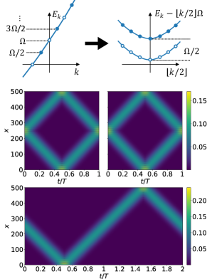
Figure 2: Top left: when the drive frequency matches twice the typical level spacing (i.e. an $s=2,r=1$ resonance), the drive only couples $k$ of the same parity (solid or empty dots). The effective model becomes two independent chains with an overall $\Omega/2$ gap between their “onsite” potentials (top right). Center: A twin pair of $s=2,r=1$ wave packet solutions of Eq. 6 ($L=500,g=1,T=225$), corresponding to the respective ground states of the two effective chains. Their spatial-temporal patterns are almost indistinguishable. Their quasienergies are $\pi+\delta$ apart, where numerically $\delta\sim 2.6\times 10^{-6}\pi$. Bottom: dynamical evolution of a time-crystalline wave packet initialized as the sum of the two solutions, undergoing $r=1$ round trip in $s=2$ drive periods. After an very long tunneling time of $2\pi T/\delta\sim 7.6\times 10^{5}T$, it would evolve into the wave packet configuration of the opposite linear combination (difference instead of sum).

For $s>1,r=1$, we consider $s=2$ as a concrete example. To leading order, the drive only resonantly couples within even $k=2\kappa$ and odd $k=2\kappa+1$, separately. One can thus use an ansatz similar to Eq. 4 but restricted to a given parity, $|\psi^{(\sigma)}(t)\rangle=\sum_{\kappa}f_{\kappa}^{\sigma}|\varepsilon_{2\kappa+\sigma}\rangle e^{-i\kappa\Omega t}$, where $\sigma=0,1$ is the parity of $k$. Invoking Eq. 2 then leads to two effective lattice models similar to Eq. 5, one for each parity, see SM. Similar to the primary resonance case, one then concludes that wave packet solutions generically exist above a crossover drive strength. Crucially, at large $L$, the two effective chains are essentially identical except for an overall $\frac{\Omega}{2}$ shift in the “onsite” energy (Fig. 2 top). This translates to a $\pi$ gap between their quasienergy spectra, and is the origin of time-crystalline nature of individual wave packets, as we will see next.

In Fig. 2 (center), we plot two $(s,r)=(2,1)$ wave packet solutions resulting from Eq. 6, which correspond to the “ground state” of the even- and odd-parity effective models, respectively. As shown, both consist of two counter-propagating wave packets that evolve into each other after one period. Thus, even though the individual wave packet returns only after $2T$, the Floquet eigenstate remains $T$-periodic. Individual wave packet can be obtained by initializing into the sum (or difference) of the two parity ground states. The evolution of one such combination is shown in Fig. 2 (bottom). As mentioned before, the quasienergy gap between the two parity-related states is $\pi+\delta$, where the small deviation $\delta$ is due to higher order effects that mix the two parity sectors. In the limit $\delta\rightarrow 0$, the individual wave packets are perfectly stable, recurring after $2T$ – a manifestation of time-translation symmetry breaking, analogous to discrete time crystals. A nonzero $\delta$ introduces a time scale $2\pi T/\delta$, over which one time translation symmetry-broken state tunnels into the other. We find numerically that this tunnelling time can be indeed very long, reaching thousands of drive periods for reasonable drive strengths and system sizes, and is easily tunable. For Fig. 2, the tunneling time is $\sim 10^{5}T$.

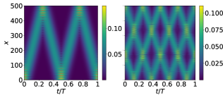
Figure 3: Floquet wave packets at generic $(s,r)$ resonances, coexisting under the same drive Eq. 6 with $L=500,g=1,T=1005$ (same as Fig. 1). Such Floquet states consist of $s$ traveling wave packets, each traversing $r$ round trips in $s$ drive periods. Left: $s=1,r=2$. Right: $s=3,r=4$.

We note that time-crystallinity is typically discussed in the context of interacting many body systems. The Floquet wave packets here are single particle states, and their “time crystallinity” refers only to their time-translation symmetry breaking behavior. Nevertheless, we expect that such behavior would survive also in the many-body setting in the presence of interaction; this will be a subject of future work Note (2).

The analysis with $r>1$ is technically more involved, and we leave mathematical details to the SM, where we discuss a nontrivial generalization of the “degenerate perturbation” ansatz Eq. 4 and the resulting effective lattice model (a more elaborate version of Eq. 7). We find that an $(s,r)$ Floquet eigenstate consists of $s$ wave packets, each completing a fraction $\frac{r}{s}$ of round trip in one drive period, see Fig. 3. Like the $s=2$ case discussed before, a given $(s,r)$ solution is one of $s$ partners with almost identical spatial-temporal patterns, and their quasienergies are equally spaced by $\Delta\theta=2\pi/s$ to leading order. The individual wave packets can be resolved by linear combinations of the $s$ partners, hence their true recurrence time is $2\pi/\Delta\theta=sT$. However, since they completed $r$ round trips in $sT$, their apparent recurrence time is $T_{\text{rec}}=sT/r$. The rational ratio of $T_{\text{rec}}/T$ is suggestive of a fractional time crystalline order, a notion put forward very recently Matus and Sacha (2019); Pizzi et al. (2019).

Floquet drive engineering

Finally, we discuss how to realize a desired target micromotion through drive engineering. Assume the time-dependent Hamiltonian has a form $\hat{H}(t)=\sum_{n}w_{n}Q_{n}(t)+h.c.$ where $Q_{n}=\hat{h}_{n}e^{ia_{n}\Omega t}$ represent experimentally available Hamiltonian controls $\hat{h}_{n}$ at integer harmonics $a_{n}$, and $w_{n}$ are (generally) complex-valued coefficients. Given a target micromotion $|\tilde{\psi}(t)\rangle$ and a prescribed set of $\{Q_{n}\}$, one can ask what is the best choice of $\{w_{n}\}$ to produce a micromotion as close to the target as possible. Writing the Floquet-Schrödinger operator as $K=\hat{H}(t)-Q_{0}$ where $Q_{0}=i\partial_{t}$, the optimal coefficients are those that minimize the variance $\Delta=\langle K^{2}\rangle_{c}$, where $\langle\mathcal{O}\mathcal{O}^{\prime}\rangle_{c}=\langle\mathcal{O}\mathcal{O}^{\prime}\rangle-\langle\mathcal{O}\rangle\langle\mathcal{O}^{\prime}\rangle$ and $\langle\mathcal{O}\rangle=\int_{0}^{T}dt\langle\tilde{\psi}|\mathcal{O}|\tilde{\psi}\rangle$. By construction, $\Delta\geq 0$ and vanishes only if $|\tilde{\psi}\rangle$ is an exact eigenstate of $K$ Qi and Ranard (2019); Chertkov and Clark (2018); Greiter et al. (2018). Demanding $0=\frac{\partial\Delta}{\partial w_{n}}=\frac{\partial\Delta}{\partial w_{n}^{*}}$ then yields the solution $\left(\begin{smallmatrix}{\boldsymbol{w}}\\ {\boldsymbol{w}}^{*}\end{smallmatrix}\right)=\left(\begin{smallmatrix}G&F\\ F^{*}&G^{*}\end{smallmatrix}\right)^{-1}\left(\begin{smallmatrix}{\boldsymbol{J}}\\ {\boldsymbol{J}}^{*}\end{smallmatrix}\right)$, where $G_{mn}=\langle Q_{m}Q_{n}+Q_{n}Q_{m}\rangle_{c}$, $F_{mn}=\langle Q_{m}Q_{n}^{\dagger}+Q_{n}^{\dagger}Q_{m}+h.c.\rangle_{c}$, $J_{n}=\langle Q_{0}Q_{n}+Q_{n}Q_{0}\rangle_{c}$, and $(\cdot)^{-1}$ is the Moore-Penrose pseudo-inverse. As a proof of principle, we target a non-dispersing Gaussian wave packet, $|\tilde{\psi}(t)\rangle=\sum_{k}\tilde{f}_{k}|k\rangle e^{-ik\Omega t}$ where $\tilde{f}_{k}\propto e^{-(k-k_{0})/4\sigma^{2}}$. On a chain of length $L=100$, for example, we can realize this wave packet as a Floquet eigenstate (to a high fidelity of $>0.99$ at all time) using only on-site drives and only two frequencies (i.e. the first and second harmonic); see Fig. 4. In contrast, the static Hamiltonian necessary to sustain such a dynamically non-dispersing wave packet, $\sum_{k}|k\rangle k\Omega\langle k|$, is spatially highly nonlocal. Note that targeting a different micromotion (e.g., one with different $k_{0}$ and $\sigma$) generally results in a different optimal drive. Fidelity with the target state can be further enhanced with more drive terms such as local hops or higher harmonic modulations. Additional requirements such as spatial smoothness of the drive can be implemented by including corresponding penalty terms in $\Delta$.

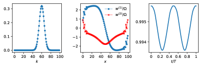
Figure 4: Optimal drive to reproduce a target micromotion $|\tilde{\psi}(t)\rangle=\sum_{k}e^{-(k-k_{0})/4\sigma^{2}-ik\Omega t}|\varepsilon_{k}\rangle$ on a chain of length $L=100$, with $k_{0}=60$ and $\sigma^{2}=15$. We use static, translation-invariant nearest neighbor hopping, and onsite modulation up to the second harmonic, $\hat{H}(t)=\sum_{x}w^{(0)}|x\rangle\langle x+1|+[w_{x}^{(1)}e^{i\Omega t}+w_{x}^{(2)}e^{2i\Omega t}]|x\rangle\langle x|+h.c$. Left: $k$-space Gaussian profile of the target state. Center: optimal drive strengths; the optimal static hopping is $w^{(0)}/\Omega=17.09$. Note that all $w$ numerically turn out to be real-valued even though they are allowed to be complex. Right: Fidelity $|\langle\tilde{\psi}|\psi\rangle|$ between reproduced and target micromotions over one period.

Discussion

We note in closing that effective models like Eq. 5 allow us to efficiently reason about more complicated drives. For example, in Eq. 6, while keeping the temporal profile as $\cos(\Omega t)$, one could replace the single site modulation with $\sum_{x}v(x)|x\rangle\langle x|$ of an arbitrary—potentially fully random—spatial profile $v(x)$, yet the product form $g_{k^{\prime}-k}V_{kk^{\prime}}$ in Eq. 5 automatically filters out all but one Fourier component in $v(x)$, hence its only effect is to renormalize the drive strength. This implies, among other things, that the resulting wave packets do not perceive any spatial randomness in the drive. On the other hand, if one fine-tunes $v(x)$ such that a particular spatial Fourier component vanishes exactly, then the corresponding resonance will be fully suppressed.

The compact wave packets reported here are closely related to spatio-temporal focusing that leads to pulse formation in long parametrically modulated resonators, such as mode-locked lasers. In the case of perfectly linear dispersion (as for electromagnetic waves in vacuum), parametric pumping leads to exponential amplification and spatial compression of any initial field configuration Martin (2019); in the tight binding model discussed here, the exponential explosion is truncated due to the energy dependence of group velocity, leading instead to formation of compact travelling Floquet eigenstates.

Acknowledgment

We are grateful to Ian Mondragon-Shem, D. Schuster, V. Manucharyan, A. V. Balatsky, A. Saxena, and D. P. Arovas for useful discussions and feedbacks. This material is based upon work supported by Laboratory Directed Research and Development (LDRD) funding from Argonne National Laboratory, provided by the Director, Office of Science, of the U.S. Department of Energy under Contract No. DE-AC02-06CH11357

Appendix A Supplemental Materials

In this note, we provide details on the analysis of $r\neq s\neq 1$ Floquet wave packets. We first discuss analytically tractable cases where one of $r$ and $s$ is $1$. When neither of them is $1$, an effective lattice model can still be derived, although it does not yield to analytical solution, and we discuss its qualitative features. We then briefly discuss the special case where the Floquet drive resonates with the undriven energy spectrum close to its inflection point, which leads to an effective lattice model with a cubic “potential”. Finally we estimate the change in the width of the wave packets during one period.

Appendix B Effective model for $s>1,r=1$

In this section, we discuss the effective model for the $s>1,r=1$ resonance, where the drive frequency matches $s$ times the typical level spacing, $\Omega\simeq s\Delta$. A generic undriven energy spectrum can be expanded as ($k_{*}$ not integer in general)

$$\varepsilon_{k}=\varepsilon_{k_{*}}+(k-k_{*})\frac{\Omega}{s}+\frac{u}{T}(k-k_{*})^{2}+\cdots\ .$$ (8)

To leading order, the drive only resonantly couples level $k$ to $k\pm s$. This effectively separates the undriven energy eigenstates into $s$ subspaces according to $\sigma=k\mod s$. For example, when $s=2$, $\sigma=0,1$ is the parity of $k$, and to leading order, the drive does not mix states of different parity. Writing

$$k=\kappa s+\sigma\ ,$$ (9)

then within each subspace $\sigma$, the integer $\kappa$ plays the role of $k$ in primary resonance, hence we can use an ansatz

$$|\psi^{\sigma}(t)\rangle=\sum_{\kappa}f_{\kappa}^{\sigma}|\varepsilon_{\kappa,\sigma}\rangle e^{-i\kappa\Omega t}\ .$$ (10)

Note that when $s=1$, $\sigma$ can only be $0$, and the ansatz above reduces to that of the primary resonance discussed in the text. Recall that the Floquet-Schrodinger equation is

$$\left[\hat{H}(t)-i\partial_{t}\right]|\psi(t)\rangle=\frac{\theta}{T}|\psi(t)\rangle\ ,$$ (11)

where the time-dependent Hamiltonian is

$$\hat{H}(t)=\hat{H}_{0}+\hat{V}(t)\quad,\quad\hat{V}(t)=\sum_{a}g_{a}\hat{V}^{(a)}e^{ia\Omega t}\ .$$ (12)

Solving Eq. 11 with 10 then yields an eigenvalue equation

$$\sum_{\kappa^{\prime}}\left[s^{2}u(\kappa-\kappa_{*}^{\sigma})^{2}\delta_{\kappa\kappa^{\prime}}+g_{\kappa^{\prime}-\kappa}V^{\sigma}_{\kappa\kappa^{\prime}}\right]f_{\kappa^{\prime}}^{\sigma}=(\theta^{\sigma}-\theta^{\sigma}_{*})f_{\kappa}^{\sigma}\ ,$$ (13)

where

$$V_{\kappa\kappa^{\prime}}^{\sigma}=\langle\varepsilon_{\kappa,\sigma}|\hat{V}^{(\kappa^{\prime}-\kappa)}|\varepsilon_{\kappa^{\prime},\sigma}\rangle T\quad,\quad\kappa_{*}^{\sigma}=\frac{k_{*}-\sigma}{s}\quad,\quad\theta^{\sigma}_{*}=\varepsilon_{k_{*}}T-2\pi\kappa_{*}^{\sigma}\ .$$ (14)

The effective model, Eq. 13, thus consists of $s$ independent “chains”, where $\sigma$ labels the chains, and $\kappa$ labels “sites” within each chain. The “onsite potential” is quadratic, $u(\kappa-\kappa_{*}^{\sigma})^{2}$, and each chain has its own quasienergy shift (i.e., a chain-dependent “chemical potential”) $\theta_{*}^{\sigma}$.

In a large system with $L$ physical sites, $V^{\sigma}_{\kappa\kappa^{\prime}}$ becomes $\sigma$-independent (The leading order correction due to finite $L$ is $\sim L^{-1}$. E.g., in an open boundary chain, it comes from $\delta q_{k}\frac{\partial}{\partial q_{k}}|\varepsilon_{k}\rangle$ where $q_{k}=\frac{k\pi}{L+1}$ is the wave vector in an open boundary chain, and $\delta q_{k}=q_{k+1}-q_{k}\propto L^{-1}$). Hence Eq. 13 for different $\sigma$ have the same set of eigenvalues $\{\theta^{\sigma}-\theta^{\sigma}_{*}\}$. The quasienergies $\{\theta^{\sigma}\}$ from different chains $\sigma$ are thus “gapped” from each other by $\theta^{\sigma+1}_{*}-\theta^{\sigma}_{*}=\frac{2\pi}{s}$, but otherwise identical. In other words, the $i^{th}$ quasienergy on “chain” $\sigma$ is $\theta_{i}^{\sigma}=\theta_{i}^{0}+\frac{2\pi\sigma}{s}$, where $\theta_{i}^{0}$ is the $i^{th}$ quasienergy on “chain” $\sigma=0$. Thus with the same index $i$, there are $s$ Floquet eigenstates with different $\sigma$ labels whose quasienergies are equally spaced by $\Delta\theta=2\pi/s$. The time evolution of an arbitrary linear superposition of these Floquet eigenstates thus have a recurrence time of $2\pi T/\Delta\theta=sT$. Such recombined states manifestly break the time translation symmetry of the driving Hamiltonian, which is periodic in $T$, and are thus single particle analogues of discrete time crystals.

Let us now discuss the spatial feature of these Floquet eigenstates and their time-crystalline linear recombinations, assuming the undriven states are momentum eigenstates of an open boundary chain, $\langle x|\varepsilon_{k}\rangle=\sqrt{\frac{2}{L+1}}\sin(q_{k}x)$ where the wave vectors are $q_{k}=k\frac{\pi}{L+1}$. A Floquet eigenstate $|\psi^{\sigma}\rangle$ of a given $\sigma$ (Eq. 10) is a linear combination of momentum states with the same $\sigma$, and are therefore invariant under spatial translation by $2L/s$ (with phase shift $2\pi\sigma/s$), where the system size $L$ is half the round trip length. To conform with this translation symmetry, $|\psi^{\sigma}\rangle$ for any $\sigma$ must consist of $s$ spatial packets equally spaced along the round trip. To resolve these spatial packets, we Fourier transform the set of $\{|\psi^{\sigma}\rangle\}$ states at $t=0$,

$$|\phi^{\lambda}\rangle=\sum_{\sigma=0}^{s-1}e^{-i2\pi\lambda\sigma/s}|\psi^{\sigma}(0)\rangle\quad,\quad\lambda=0,1,\cdots,s-1\ .$$ (15)

As discussed before, in the limit where the level spacing of the quasienergies $\Delta\theta=2\pi/s$ is exact (i.e., when (1) we ignore higher order effect of the drive that mixes different $\sigma$ sectors, and (2) $V^{\sigma}_{\kappa\kappa^{\prime}}$ becomes $\sigma$-independent at large $L$), any linear combination of $\{|\psi^{\sigma}\rangle\}$ breaks the discrete time translation symmetry of the driving Hamiltonian. For $|\phi^{\lambda}\rangle$, we have

$$\hat{U}_{T}|\phi^{\lambda}\rangle=e^{-i\theta^{0}}|\phi^{\lambda+1}\rangle\implies\hat{U}_{sT}|\phi^{\lambda}\rangle=e^{-is\theta^{0}}|\phi^{\lambda}\rangle\ ,$$ (16)

where $\hat{U}_{sT}$ is dynamical time evolution over $s$ drive periods. In other words, the $|\phi^{\lambda}\rangle$ states evolve into each other after one $T$, and recur after $sT$. Physically, each $|\phi^{\lambda}\rangle$ corresponds to a single spatial packet that propagates by $2L/s$ after $T$, and completes a round trip of length $2L$ after $sT$.

Numerically, the quasienergy spacing among the $s$ partners $\{|\psi^{\sigma}\rangle\}$ is $\Delta\theta=2\pi/s+\delta$, where a small $\delta$ originates from higher order effect of the drive that mixes different $\sigma$ sectors, as well as the $\sigma$ dependence in $V^{\sigma}_{\kappa\kappa^{\prime}}$. Consequently, the $|\phi^{\lambda}\rangle$ states will “tunnel” among the $s$ wave packet configurations over a time scale of $2\pi T/\delta$. Numerically, the tunneling time is typically of the order of thousands of drive periods, and may be extended further via parameter fine tuning.

When $\hat{V}(t)=2g\cos\Omega t|1\rangle\langle 1|$, i.e., a modulation on the first site at the fundamental frequency, the effective model Eq. 13 of a given $\sigma$ becomes a lattice version of harmonic oscillator,

$$s^{2}u(\kappa-\kappa_{*}^{\sigma})^{2}f_{\kappa}^{\sigma}+\tau(f_{\kappa-1}^{\sigma}+f_{\kappa+1}^{\sigma})=(\theta^{\sigma}-\theta^{\sigma}_{*})f_{\kappa}^{\sigma}\ ,$$ (17)

where the parameters $u$ and $\tau$ can be estimated using $\partial_{k}\varepsilon_{k_{*}}=\Omega/s$ and $\partial^{2}_{k}\varepsilon_{k_{*}}=2s^{2}u/T$,

$$u=\frac{\pi^{2}}{\mathcal{L}^{2}}\sqrt{T^{2}-\mathcal{L}^{2}/s^{2}}\quad,\quad\tau=\frac{2g}{s^{2}}\frac{\mathcal{L}}{T}\ .$$ (18)

Here $\mathcal{L}=L+1$. Note that the effective stiffness is now $s^{2}u$. Parametrizing

$$\beta_{s}=\frac{\mathcal{L}}{sT}\quad,\quad\gamma_{s}=\frac{1}{\sqrt{1-\beta_{s}^{2}}}\ ,$$ (19)

then similar to the primary resonance case, one can estimate the emergent oscillator “frequency” $\varpi_{s}$ and the number of wave packet solutions (per $\sigma$) $D_{s}$ as

$$\varpi_{s}=2\sqrt{s^{2}u\tau}=2\pi\sqrt{\frac{2g}{\gamma_{s}\mathcal{L}}}\quad,\quad D_{s}\simeq 2\sqrt{\frac{\tau}{s^{2}u}}=\frac{2\beta_{s}}{s\pi}\sqrt{2g\gamma_{s}\mathcal{L}}\ .$$ (20)

These reduce to the primary resonance results of the main text when $s=1$. The crossover drive strength $g_{c}^{(s)}$ to induce any $s>1,r=1$ wave packet solution at all is

$$D_{s}(g_{c}^{(s)})=1\implies g_{c}^{(s)}=\frac{s^{2}\pi^{2}}{8\beta_{s}^{2}\gamma_{s}\mathcal{L}}\ .$$ (21)

Thus one generally needs a stronger drive to induce wave packets of larger $s$.

Appendix C Effective model for $r>1,s=1$

The situation with $r>1$ is more involved. Consider first $s=1$, then it takes $r$ drive quanta at frequency $\Omega$ to resonantly connect two adjacent energy levels, as they have a spacing $\sim r\Omega$. As a result, a “degenerate perturbation” ansatz similar to Eq. 4 in the main text would not work: the Floquet-Schrödinger operator simply does not have matrix element between $|\varepsilon_{k}\rangle e^{-irk\Omega t}$ and $|\varepsilon_{k+1}\rangle e^{-ir(k+1)\Omega t}$. In principle, one could attempt to derive an effective coupling between these levels via an $r^{th}$ order perturbation theory; this is however technically unwieldy.

We instead take an alternate route. We are interested in wave packets which traverse $r$ round trips of an $L$-site system in a single drive period. Heuristically, this can be “unfolded” into one round trip in a system of length $rL$—much like how the trajectory of a billiard ball bouncing off the pool table can be “unfolded” into a straight line across a repetitive tile of tables. This suggests that a proper ansatz should additionally include eigenstates of the unfolded system, truncated to a segment of length $L$. These correspond to fractional momentum states $|k+\frac{\rho}{r}\rangle$ in the original system ($\rho=0,1,\cdots,r-1$); for the open chain considered before, $\langle x|k+\frac{\rho}{r}\rangle\propto\sin(q_{k+\frac{\rho}{r}}x+\varphi)$, where $\varphi$ is a phase shift depending on how the shorter system is embedded into the longer one. For drives localized on $x=1$, as we will show, $\varphi$ is such that $\langle L+1|k+\frac{\rho}{r}\rangle=0$.

In the remainder of this section, we first justify the use of fractional momentum states from perturbation theory, and then analyze a generalized ansatz that additionally includes these states.

C.1 The origin of fractional momentum states

We argued that when the drive frequency matches $1/r$ of typical level spacing of a tight binding chain of length $L$, the ansatz for Floquet eigenstates should additionally include fractional momentum states, which are energy eigenstates not of a system of length $L$, but rather of length $rL$. We now show that such fractional momentum states do emerge as the leading order correction to undriven Floquet eigenstates (the integer momentum states) when the Floquet drive is treated as a perturbation. From the perspective of variational solutions, thus, the purpose of including fractional momentum states in the generalized ansatz is so that the variational subspace remains invariant (to leading order) upon the action of the drive.

We first note that the Floquet-Schrodinger operator,

$$K=K_{0}+\hat{V}(t)\quad,\quad K_{0}=\hat{H}_{0}-i\partial_{t}\ ,$$ (22)

acts on the tensor product space of the physical Hilbert space and the space of periodic functions. The eigenvectors of $K_{0}$ (which are space-time modes) form a complete basis in this space,

$$|k,a\rangle\equiv|\varepsilon_{k}\rangle e^{-ia\Omega t}\quad,\quad K_{0}|k,a\rangle=\varepsilon_{k}-a\Omega\ ,$$ (23)

where $|\varepsilon_{k}\rangle$ are eigenstates of the undriven Hamiltonian, $\hat{H}_{0}=\sum_{x=1}^{L-1}|x\rangle\langle x+1|+h.c.$,

$$\hat{H}_{0}|\varepsilon_{k}\rangle=\varepsilon_{k}|\varepsilon_{k}\rangle\quad,\quad\varepsilon_{k}=2\cos q_{k}\ ,$$ (24)

$$\langle x|\varepsilon_{k}\rangle=\sqrt{\frac{2}{\mathcal{L}}}\sin(q_{k}x)\quad,\quad q_{k}=k\frac{\pi}{\mathcal{L}}\quad,\quad k,x=1,2,\cdots,L\quad,\quad\mathcal{L}=L+1\ .$$ (25)

Note that the frequency index $a$ in $|k,a\rangle$ is independent of the momentum index $k$. This is unlike the ansatz we used in the main text, which associates to each momentum index a specific frequency index (e.g., $a=k$ for primary resonance) — that is, the ansatz amounts to a variational solution in a subspace (of the full tensor product space) in which frequency and momentum are correlated.

Given an operator $Q=Q_{0}+Q_{1}$, and unperturbed basis $|n\rangle$ with $Q_{0}|n\rangle=\lambda_{n}|n\rangle$, the first order correction to the eigenvectors $|n\rangle$ are

$$|n^{(1)}\rangle=\sum_{m\neq n}\frac{\langle m|Q_{1}|n\rangle}{\lambda_{n}-\lambda_{m}}|m\rangle\ .$$ (26)

Now consider a Floquet drive

$$\hat{V}(t)=2g\cos(\Omega t)\hat{v}\ ,$$ (27)

Treating $\hat{V}(t)$ as a perturbation to $K_{0}$, we obtain the first order correction to the undriven modes as

$$|k,a^{(1)}\rangle=g\sum_{\begin{subarray}{c}(k^{\prime},a^{\prime})\\ \neq(k,a)\end{subarray}}\frac{\langle\varepsilon_{k^{\prime}}|\hat{v}|\varepsilon_{k}\rangle\langle a^{\prime}|2\cos(\Omega t)|a\rangle}{\varepsilon_{k}-\varepsilon_{k^{\prime}}+(a-a^{\prime})\Omega}|k^{\prime},a^{\prime}\rangle=\check{g}\sum_{\rho=\pm 1}|\chi_{k,\rho}\rangle e^{-i(a+\rho)\Omega t}\ ,$$

$$|\chi_{k,\rho}\rangle=\sum_{k^{\prime}}\frac{\langle\varepsilon_{k^{\prime}}|\hat{v}|\varepsilon_{k}\rangle}{(\varepsilon_{k}-\rho\Omega)-\varepsilon_{k^{\prime}}}|k^{\prime}\rangle\ ,$$ (28)

where $\langle a^{\prime}|f(t)|a\rangle=\int_{0}^{T}\frac{dt}{T}\,e^{i(a^{\prime}-a)\Omega t}f(t)$. Since we are considering a near resonance where the drive frequency $\Omega$ matches $1/r$ of typical level spacing, $\varepsilon_{k}-\rho\Omega$ is roughly the interpolation of the dispersion relation $\varepsilon_{k}=2\cos q_{k}$ at a fractional momentum $\kappa_{k,\rho}$,

$$\varepsilon_{k}-\rho\Omega\simeq\varepsilon_{\kappa_{k,\rho}}\quad,\quad\kappa_{k,\rho}=k+\frac{\rho}{r}$$ (29)

Let us specialize to $\hat{v}=|L\rangle\langle L|$, i.e., a drive on the last site on the chain, instead of the first site (as used in the main text). This choice is for notational convenience only, and we will comment on what changes if the drive is placed on the first site later. Using $\langle\varepsilon_{k^{\prime}}|\hat{v}|\varepsilon_{k}\rangle=\frac{2}{\mathcal{L}}(-1)^{k+k^{\prime}}\sin q_{k}\sin q_{k^{\prime}}$, we have

$$|\chi_{k,\rho}\rangle=(-1)^{k+1}\sin q_{k}\left[\frac{2}{\mathcal{L}}(-1)^{k^{\prime}}\sum_{k^{\prime}}\frac{\sin q_{k^{\prime}}}{\varepsilon_{k^{\prime}}-\varepsilon_{\kappa_{\rho}}}|k^{\prime}\rangle\right]\ .$$ (30)

We now show that $|\chi_{k,\rho}\rangle$ are indeed proportional to fractional momentum states $|\kappa\rangle$, which are defined as the interpolation of the integer momentum states (Eq. 25) to non-integer momentum “index” $\kappa$,

$$\langle x|\kappa\rangle=\sqrt{\frac{2}{\mathcal{L}}}\sin(q_{\kappa}x)\quad,\quad q_{\kappa}=\kappa\frac{\pi}{\mathcal{L}}\ \forall\kappa\ .$$ (31)

The overlap of two such states is

$$\langle\kappa^{\prime}|\kappa\rangle=I(\kappa-\kappa^{\prime})-I(\kappa+\kappa^{\prime})\ ,$$ (32)

$$I(\eta)\equiv\frac{1}{\mathcal{L}}\sum_{x=1}^{L}\cos\frac{\eta\pi x}{\mathcal{L}}=\frac{1}{2\mathcal{L}}\left[\sin(\eta\pi)\cot\frac{\eta\pi}{2\mathcal{L}}-\cos(\eta\pi)-1\right]\ .$$ (33)

Setting $\kappa^{\prime}$ to integer yields the expansion of $|\kappa\rangle$ in the integer momentum basis,

$$\langle\varepsilon_{k}|\kappa\rangle=\frac{(-1)^{k}}{\mathcal{L}}\frac{\sin(\kappa\pi)\sin q_{k}}{\cos q_{k}-\cos q_{\kappa}}\ .$$ (34)

Comparing with Eq. 30 and noting that $\cos q_{\kappa}=\frac{1}{2}\varepsilon_{\kappa}$, we find that indeed $|\chi_{\kappa,\rho}\rangle$ are fractional momentum states,

$$|\chi_{k,\rho}\rangle=(-1)^{k+1}\frac{\sin q_{k}}{\sin(\kappa_{k,\rho}\pi)}|\kappa_{k,\rho}\rangle\ .$$ (35)

The effect of the Floquet drive on the undriven modes $|k,a\rangle=|\varepsilon_{k}\rangle e^{-ia\Omega t}$ is thus to bring an integer momentum state $|k\rangle$ at frequency $a$ to fractional momenta $|k\pm\frac{1}{r}\rangle$ at neighboring frequencies $a\pm 1$.

Note that in the case of primary resonance, viz., $r=\rho=1$, the drive brings $|k,a\rangle$ to $|k\pm 1,a\pm 1\rangle$. In other words, the $k=a$ subspace remains invariant under the drive, which justifies the ansatz used in the text, $|\psi(t)\rangle=\sum_{k}f_{k}|\varepsilon_{k}\rangle e^{-ik\Omega t}$.

What if we place the drive on the first site instead of the last one? This is equivalent to relabeling site $x$ to $L+1-x$, hence the appropriate fractional momentum states $|\widetilde{\kappa}\rangle$ are related to $|\kappa\rangle$ (the ones arising from a last site drive) by $\langle x|\widetilde{\kappa}\rangle=\langle L+1-x|\kappa\rangle$. This effectively shifts $|\widetilde{\kappa}\rangle$ to a different boundary condition, $\langle x|\widetilde{\kappa}\rangle\propto\sin(q_{\kappa}x+\varphi)$ where $\varphi$ is such that $\langle L+1|\widetilde{\kappa}\rangle=0$.

C.2 Generalized ansatz and effective model

We now discuss the effective model for the $r>1,s=1$ resonance, where the drive frequency matches a fraction of the typical level spacing, $\Omega\simeq\frac{\Delta}{r}$. From a group velocity consideration, in one drive period, a wave packet consisting of states from this part of the undriven spectrum (assuming it can be stabilized) will undergo $r$ round trips (i.e., $2rL$ for an open chain of length $L$). Earlier in this section, we argued that the $r$ round trips can be “unfolded” into one round trip in a system of size $rL$, hence a proper Floquet ansatz should additionally include fractional momentum states. We also showed that such fractional momentum states naturally emerge as leading order corrections to the integer momentum states for the $r>1$ resonances. Taking these into consideration, the proper ansatz is

$$|\psi(t)\rangle=\sum_{k}\sum_{\rho=0}^{r-1}f_{k,\rho}|k+\frac{\rho}{r}\rangle e^{-i(rk+\rho)\Omega t}\ ,$$ (36)

where $|k+\frac{\rho}{r}\rangle$ are the fractional momentum states Eq. 31. Note that their average energies do not fall on the dispersion curve of the integer momentum states. Instead, one has ($\kappa=k+\frac{\rho}{r}$)

$$\langle\kappa|\hat{H}_{0}|\kappa\rangle=2\sum_{x=1}^{L-1}\langle\kappa|x\rangle\langle x+1|\kappa\rangle=2\cos q_{\kappa}\left\{1+\frac{1}{\mathcal{L}}\left[\frac{\sin(2q_{\kappa}-2\kappa\pi)}{\sin(2q_{\kappa})}-1\right]\right\}\ ,$$ (37)

$$\langle\kappa|\kappa\rangle=1-\frac{\sin\kappa\pi}{\mathcal{L}\sin q_{\kappa}}\cos(\kappa\pi-q_{\kappa})\ ,$$ (38)

hence the energy of $|\kappa\rangle$ is

$$\langle E\rangle_{\kappa}=\frac{\langle\kappa|\hat{H}_{0}|\kappa\rangle}{\langle\kappa|\kappa\rangle}=E_{\kappa}+\mu_{\kappa}\ ,$$ (40)

$$\mu_{\kappa}=\frac{1}{\mathcal{L}}\left[\cos(q_{\kappa}-2\kappa\pi)-\cos q_{\kappa})\right]+\mathcal{O}(\mathcal{L}^{-2})\ ,$$ (41)

where $E_{\kappa}=2\cos q_{\kappa}$ is the the dispersion relation of the integer momentum states, and $\mu_{\kappa}$ is the deviation $\langle E\rangle_{\kappa}-E_{\kappa}$.

Close to resonance, one can expand the (integer-$k$) dispersion relation as

$$\varepsilon_{k}=\varepsilon_{*}+r(k-k_{*})\Omega+\frac{u}{T}(k-k_{*})^{2}+\cdots\ .$$ (42)

It is useful to simplify $\mu_{\kappa}$ by replacing, in Eq. 41, $q_{\kappa}\rightarrow q_{*}$ (where $q_{*}=q_{k_{*}}=k_{*}\pi/\mathcal{L}$ is the interpolated wave vector at the resonance center $k_{*}$), and $2\kappa\pi\rightarrow 2\pi\frac{\rho}{r}$, yielding

$$\mu_{\rho}=\frac{1}{\mathcal{L}}\left[\cos(q_{*}-2\pi\frac{\rho}{r})-\cos q_{*}\right]\ ,$$ (43)

i.e., the deviation $\mu_{\rho}$ depends only on the fractional part $\rho$. Introduce a composite index

$$j=rk+\rho\ ,$$ (44)

$j$ labels the integer momentum states in the unfolded system (length $rL$). Then invoking Eq. 11 on Eq. 36 leads to the following eigenvalue problem,

$$\sum_{j^{\prime}}\left[\vartheta_{j}\delta_{jj^{\prime}}+g_{j-j^{\prime}}V_{jj^{\prime}}\right]f_{j^{\prime}}=(\theta-\theta_{*})f_{j}\ ,$$ (45)

where

$$\vartheta_{j}=\mu_{\rho}+u(\frac{j}{r}-k_{*})^{2}\quad,\quad V_{jj^{\prime}}=\langle k+\frac{\rho}{r}|\hat{V}^{(j^{\prime}-j)}|k^{\prime}+\frac{\rho^{\prime}}{r}\rangle T\quad,\quad\theta_{*}=\varepsilon_{*}T-2\pi rk_{*}$$ (46)

The effective model is thus a 1D “lattice” with “unit cell” label $k$ and “sublattice” label $\rho$. The “onsite potential” $\vartheta$ remains quadratic, but has an additional sublattice-dependent “chemical potential” $\mu_{\rho}$.

Before analyzing the effective model, we first discuss why the apparent recurrence time of the wave packet solutions for $r>1$ is $T/r$. This behavior can be understood from the form of the ansatz. Note that $|\psi(t)\rangle$ in Eq. 36 can be separated into “sublattice” contributions, $|\psi(t)\rangle=\sum_{\rho}|\psi_{\rho}(t)\rangle$, where $|\psi_{\rho}(t)\rangle=\sum_{k}f_{k,\rho}|k+\frac{\rho}{r}\rangle e^{-ij(k,\rho)\Omega t}$. Since by construction, $|\psi_{\rho}(T/r)\rangle=e^{-i2\pi\rho/r}|\psi_{\rho}(0)\rangle$, each “sublattice” recur after a fraction of drive period $\frac{T}{r}$, but with different phase shift. Thus even though rigorously speaking the full state $|\psi(t)\rangle$ does not recur after $T/r$ due to the phase shifts (the exact recurrence time is $T$), its spatial pattern does approximately return after $T/r$.

We now analyze the effective model assuming the drive has the form $\hat{V}(t)=2g\cos(\Omega t)|L\rangle\langle L|$, that is, a modulation on the last site at the fundamental frequency. The reason to modulate the last (instead of the first) site is to simplify the expression for the fractional momentum states, see discussion at the end of the last section. Then the drive only couples $j$ to $j\pm 1$. The effective model becomes

$$\left[\mu_{\rho}+\frac{u}{r^{2}}\right](j-j_{*})^{2}f_{j}^{(\rho)}+\tau(f_{j+1}^{(\rho+1)}+f_{j-1}^{(\rho-1)})=\lambda f_{j}\quad,\quad$$ (47)

where $j_{*}=k_{*}/r$, $\lambda=(\theta-\theta_{*})$, and we have used the approximation that the “hopping” $\tau$ is “site”-independent. Note that we have placed a superscript $\rho$ to the coefficients $f_{j}$, where $\rho=j\mod r$ (Eq. 44), and the superscripts are understood as carrying an implicit $\mod r$ (i.e., $\rho\pm 1$ should be understood as $(\rho\pm 1)\mod r$, etc.). Let us now Fourier transform the index $j$ into a continuous conjugate variable $y$,

$$f_{j}^{(\rho)}\equiv\int dy\check{f}^{(\rho)}(y)e^{-i(j-j_{*})y}\ .$$ (48)

Note that the transformation is performed as if $\rho$ is independent of $j$. What this means is that if one were given $r$ continuous functions $\check{f}^{(\rho)}(y)$, $\rho=0,1,\cdots,r-1$, then only Fourier components with $j\equiv\rho\mod k$ are relevant as solution to Eq. 47. In terms of $\check{f}^{(\rho)}$, Eq. 47 becomes a coupled Mathieu’s equation,

$$\left[\hat{M}-\frac{u}{r^{2}}\partial_{y}^{2}\right]{\boldsymbol{\check{f}}}=\lambda{\boldsymbol{\check{f}}}\ ,$$ (49)

where

$$\hat{M}=\begin{pmatrix}\mu_{0}&\tau e^{-iy}&&&&\tau e^{iy}\\ \tau e^{iy}&\mu_{1}&\tau e^{-iy}\\ &\tau e^{iy}&\mu_{2}&\ddots\\ &&\ddots&\ddots&\ddots\\ &&&\ddots&\mu_{r-2}&\tau e^{-iy}\\ \tau e^{-iy}&&&&\tau e^{iy}&\mu_{r-1}\end{pmatrix}\quad,\quad{\boldsymbol{\check{f}}}=\begin{pmatrix}\check{f}^{(0)}\\ \check{f}^{(1)}\\ \vdots\\ \vdots\\ \vdots\\ \check{f}^{(r-1)}\end{pmatrix}$$ (50)

The general strategy is then to solve Eq. 49 in the diagonal basis of the matrix $\hat{M}$.

Since a generic $\hat{M}$ cannot be diagonalized analytically, we will specialize to $r=2$. In this case, one has

$$r=2\implies\hat{M}=\begin{pmatrix}\mu_{0}&2\tau\cos(y)\\ 2\tau\cos(y)&\mu_{1}\end{pmatrix}\ .$$ (51)

Denoting the diagonal bases of $\hat{M}$ as $\check{f}^{\pm}(y)$, then Eq. 49 becomes

$$\left[-\frac{u}{r^{2}}\partial_{y}^{2}\pm\sqrt{\frac{\Delta\mu^{2}}{4}+4\tau^{2}\cos^{2}y}\right]\check{f}^{\pm}(y)=(\lambda^{\pm}-\bar{\mu})f^{\pm}(y)\quad,\quad\Delta\mu=\mu_{1}-\mu_{0}\quad,\quad\bar{\mu}=\frac{\mu_{0}+\mu_{1}}{2}\ .$$ (52)

The problem is equivalent to a particle moving in a periodic potential $U^{\pm}(y)=\pm\sqrt{\frac{\Delta\mu^{2}}{4}+4\tau^{2}\cos^{2}y}$. The Floquet wave packets correspond to bound states in one of the two potentials. Near the bottom of either potential, one may Taylor expand in $y$ and obtain

$$U^{+}(y)\simeq\frac{\Delta\mu}{2}+\frac{4\tau^{2}}{\Delta\mu}\delta y^{2}+\cdots\quad,\quad U^{-}(y)\simeq-\sqrt{\frac{\Delta\mu^{2}}{4}+4\tau^{2}}+\frac{2\tau^{2}}{\sqrt{\frac{\Delta\mu^{2}}{4}+4\tau^{2}}}\delta y^{2}+\cdots\ .$$ (53)

We expect Floquet wave packet solutions to be low-lying states of the effective lattice model Eq. 47 (this is because at higher quasienergies, the “hopping” cannot efficiently mix neighboring “sites”, hence the solutions there are closer to single-momentum states, which are spatially extended). This means at a weak drive strength (and hence small $\tau$), we should choose $U^{-}$ of the two potential branches, as it has a negative overall shift. The effective model is thus a continuum harmonic oscillator of “Hamiltonian”

$$\widetilde{H}=-m^{-1}\partial_{y}^{2}+q\delta y^{2}-C\ ,$$ (54)

where the “mass” $m$, the “stiffness” $q$, and the constant shift $C$ are

$$m^{-1}=\frac{u}{r^{2}}\quad,\quad q=\frac{2\tau^{2}}{C}\quad,\quad C=\sqrt{\frac{\Delta\mu^{2}}{4}+4\tau^{2}}\ .$$ (55)

The parameters $u,\tau$, and $\Delta\mu$ can be estimated as follows. Parametrizing

$$\beta_{r}=\frac{r\mathcal{L}}{T}\quad,\quad\gamma_{r}=\frac{1}{\sqrt{1-\beta_{r}^{2}}}\ ,$$ (56)

then from $\partial_{k}\varepsilon_{k}|_{k=k_{*}}=r\Omega$ and $\frac{u}{T}=\frac{1}{2}\partial_{k}^{2}\varepsilon_{k}|_{k=k_{*}}$, we have

$$u=\frac{r^{2}\pi^{2}}{\beta_{r}^{2}\gamma_{r}T}\ .$$ (57)

For $r=2$, from Eq. 46, we can estimate $\tau$ as

$$\tau=V_{j_{*},j_{*}+1}=gT\langle k_{*}|L\rangle\langle L|k_{*}+\frac{1}{2}\rangle=\frac{4g}{\gamma_{r}}\ .$$ (58)

Finally, using Eq. 43, we have

$$\Delta\mu=\mu_{1}-\mu_{0}=\frac{2T}{\mathcal{L}}\cos q_{*}=\frac{4}{\beta_{r}\gamma_{r}}\ .$$ (59)

The “frequency” of the emergent harmonic oscillator, Eq. 54, is then

$$\varpi=2\sqrt{m^{-1}q}=\frac{8\pi g}{\gamma_{r}\sqrt{r\mathcal{L}\sqrt{1+16g^{2}\beta_{r}^{2}}}}\ .$$ (60)

Note that at weak drive, $\varpi\propto g$. As the drive becomes stronger, $\varpi\propto\sqrt{g}$. This is different from the $r=1$ cases (with arbitrary $s$), where $\varpi\propto\sqrt{g}$ even at weak drive, see Eq. 20.

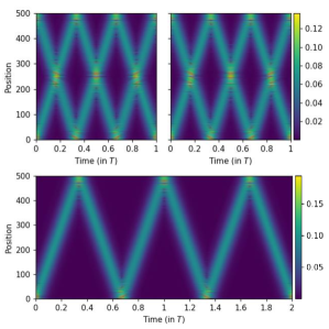
Figure 5: Non-dispersing wave packets with $s=2,r=3$ from Hamiltonian $\hat{H}(t)=\sum_{x=1}^{L-1}|x\rangle\langle x+1|+h.c.+2g\cos(\Omega t)|1\rangle\langle 1|$, with system size $L=500$, drive strength $g=1$, and drive period $T=1005$ ($\Omega=2\pi/T$). Top: “ground states” of the two parity effective chains ($\sigma=0,1$). Their Floquet phases are $\pi+\delta$ apart, and numerically $\delta\simeq 1.62\times 10^{-5}\pi$. Bottom: Dynamical evolution of the time-crystalline recombination $|\phi^{0}\rangle=|\psi^{0}(0)\rangle+|\psi^{1}(0)\rangle$. After a tunneling time of $2\pi T/\delta\simeq 1.23\times 10^{5}T$, it would evolve into the wave packet configuration of the opposite recombination $|\psi^{(0)}\rangle-|\psi^{(1)}\rangle$.

Appendix D General $r\neq s\neq 1$ wave packets

We briefly discuss the more general case of $r\neq s\neq 1$. In this case, we can combine the two ansatze above and write

$$|\psi^{\sigma}(t)\rangle=\sum_{\kappa,\rho}|k(\kappa,\rho,\sigma)\rangle e^{-i(r\kappa+\rho)\Omega t}\ ,$$ (61)

where $k(\kappa,\rho,\sigma)$ is a potentially fractional momentum,

$$k(\kappa,\rho,\sigma)=s(\kappa+\frac{\rho}{r})+\sigma\ ,$$ (62)

and $\kappa,\rho,\sigma$ are integers, with $\rho=0,1,\cdots,r$ and $\sigma=0,1,\cdots,\sigma$. Thus invoking Eq. 11 on this ansatz will yield an effective lattice model of $s$ decoupled chains (labeled by $\sigma$), each with $r$ sublattices (labeled by $\rho$). Note that each chain (i.e., a specific $\sigma$) can be analyzed in the same way as the $s=1,r>1$ case, except the index $j$ in Eq. 44 is now $j=r\kappa+\rho$ (i.e., replace $k$ there by $\kappa$). Similar to the $r=1$ case, the “onsite” energies of the $s$ chains have an equal spacing of $2\pi/s$ to leading order (with higher order corrections arising from the coupling between different $\sigma$ sectors), but otherwise essentially identical, hence a given $(s,r)$ solution is necessarily one of $s$ partners with almost identical spatial-temporal patterns, and their quasienergies are equally spaced by $\Delta\theta=2\pi/s$ to leading order. Combining the results of $s=1$ and $r=1$, one can see that at $s\neq r\neq 1$, an $(s,r)$ Floquet eigenstate consists of $s$ wave packets, each completing a fraction $\frac{r}{s}$ of round trip in one drive period. The individual wave packets can be resolved by linear recombinations of the $s$ partners, similar to Eq. 15, hence their true recurrence time is $2\pi/\Delta\theta=sT$. However, since they completed $r$ round trips in $sT$, their apparent recurrence time is $T_{\text{rec}}=sT/r$. In Fig. 5, we plot the “ground states” of the two independent effective chains for $s=2,r=3$, and their time-crystalline recombination. The latter completes $r=3$ round trips in $s=2$ drive periods.

D.1 Emergent lattice model with cubic potential

Emergence of non-dispersing Floquet wave packets does not rely on the “on-site potential” in the effective lattice model being quadratic. In this section, we discuss the case where the effective potential becomes cubic. Such a scenario would arise, for example, by fine-tuning the drive frequency to match the level spacing at the inflection point of the undriven spectrum, $T\simeq\widetilde{L}\Rightarrow q_{*}\simeq\pi$. See Fig. 6. By definition, the quadratic term in the Taylor expansion of $\varepsilon_{k}$ vanishes, and one instead has $\varepsilon_{k}=\varepsilon_{*}+\Omega(k-k_{*})+\frac{u}{T}(k-k_{*})^{3}+\cdots$. The effective lattice model is now $u(k-k_{*})^{3}f_{k}+\tau(f_{k-1}+f_{k+1})=(\theta-\theta_{*})f_{k}$, where $u=\frac{1}{6}T\frac{\partial^{3}\varepsilon_{k}}{\partial k^{3}}|_{k_{*}}=\pi^{3}/3\tilde{L}^{2}$, while $\tau$ has the same expression as in quadratic case and is $\tau=2g$. Such an arrangement can host wave packet solutions, because as long as $\tau$ is not too small, it can still efficiently couple several nearby $k$ “sites” together. The potential profile only matters in determining how many $k$ points can be coupled, and the weight distribution among them. Note that while the quantum mechanical problem of a particle in continuous space, with a purely cubic potential, has no real eigenvalues Ferreira and Sesma (2014), the discrete nature of our effective model here places a natural cutoff on the cubic potential (a “site” with too high a potential cannot couple to neighboring sites via hopping)—in other words, the potential is cubic near the center, but has effective infinite walls on both sides, hence there is no subtlety in obtaining wave packet solutions with real eigenvalues. Indeed, similar to the quadratic case, the number of wave packet states $D$ can be estimated as $u|\delta k|^{3}\leq\tau\Rightarrow|\delta k|\leq(\tau/u)^{1/3}\Rightarrow D\simeq 2(\tau/u)^{1/3}\propto(g\tilde{L}^{2})^{1/3}$. Compared with the quadratic case, these wave packets have a broader weight distribution in $k$ due to the flatter cubic potential, leading to more compact coordinate space Floquet wave packets. The crossover drive strength is obtained by having $D=2$ (instead of $1$, because the cubic model has a particle-hole symmetry), and is thus $\tau_{c}\simeq u$, or $g_{c}\propto\tilde{L}^{-2}$. To estimate the Floquet level spacing near $\theta_{*}$ (the analogue of $\varpi$ in the quadratic case), we use the effective Hamiltonian of a generic power law potential to write $\Delta\theta^{(\nu)}=u\Delta X^{\nu}+\tau\Delta K^{2}$, where $X$ and $K$ are the “position” and “translation generator” of the emergent lattice, and $\Delta X,\Delta K$ their variances. Minimizing $\Delta\theta^{(\nu)}$ under the constraint of minimal uncertainty $\Delta X\Delta K=1$ ($\hbar=1$) then leads to the level spacing

$$\varpi^{(\nu)}=\frac{\nu+2}{\nu}\tau\left[\frac{2\tau}{\nu u}\right]^{-\frac{2}{\nu+2}}\ .$$ (63)

One can verify that $\varpi^{(2)}$ recovers the quadratic emergent “frequency” $\varpi$. For the cubic case, we have $\varpi^{(3)}=\frac{5}{3}\left[\frac{3}{2}\right]^{2/5}u^{2/5}\tau^{3/5}\propto\left(g^{3}/\tilde{L}^{4}\right)^{1/5}$. Since a tight binding model with cubic potential has particle hole symmetry, its eigenvalues come in $\pm$ pairs, and the analogue of “low lying” state are those with eigenvalues close to zero (i.e., potential center). The bottom two panels in Fig. 6 plots the two lowest lying Floquet eigenstates (in the positive eigenvalue branch of the effective model).

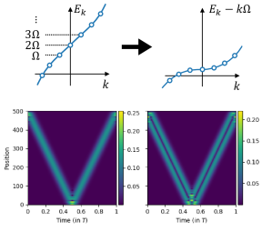
Figure 6: Non-dispersing wave packets from an effective “cubic” oscillator. When the drive frequency resonates at the inflection point of a spectrum (top left), the effective model becomes a tight binding chain with a cubic onsite potential (top right). Bottom panels: Floquet wave packet solutions corresponding to eigenstates of the effective model closest to “zero” energy (i.e., center of the cubic potential). System size $L=500$, drive strength $g=1$, drive period $T=501$ (Setting $T=L+1$ matches the drive frequency exactly at the spectral inflection point).

D.2 Change of the width of a Floquet wave packet in one drive period

In this section, we estimate how much the width of the (“ground state”) Floquet wave packet (i.e., the one with a single spatial peak) changes within one drive period. As shown in the main text, the Floquet wave packets remain spatially compact at all time. Its typical width can be estimated as

$$W\simeq\frac{L}{D}\ ,$$ (64)

where $L$ is chain length, and $D$ is the number of wave packet states, which we have estimated in the main text. This is because crudely speaking, one can think of all Floquet wave packet states as spanning the same spatial extent, hence on average, each wave packet has a spatial extent of $W$, which for the “ground state” is its width.

To estimate how much the width changes, recall that $D$ was estimated by finding how many momentum states can be efficiently coupled by the Floquet drive — the Floquet wave packets can be viewed as resulting from a “degenerate perturbation” theory in the Hilbert space spanned by these momentum states. Since we only apply drive on a single site, the wave packet propagates mostly freely when away from the drive site, hence its spread is due to the difference in velocity between the fastest and slowest momentum component. To make the discussion more general, we consider the following expansion of the (undriven) energy spectrum,

$$\varepsilon_{k}=\varepsilon_{*}+\Omega(k-k_{*})+\frac{u_{n}}{T}(k-k_{*})^{n}+\cdots\ ,$$ (65)

where $n=2,3$ give the quadratic and cubic cases discussed before. The effective lattice model is (see discussion in the main text and the previous section on the cubic case)

$$u_{n}(k-k_{*})^{n}f_{k}+\tau(f_{k-1}+f_{k+1})=(\theta-\theta_{*})f_{k}\ .$$ (66)

The number of wave packet states $D$ is estimated as the number of (integer) $k$ “sites” that can be reached from $k_{*}$ by one “hop” $\tau$,

$$u_{n}(\Delta k)^{n}=\tau\implies\Delta k=\left[\frac{\tau}{u_{n}}\right]^{1/n}\quad,\quad D=2\Delta k\ .$$ (67)

This yields

$$W\simeq\frac{L}{D}\simeq L\left[\frac{u_{n}}{\tau}\right]^{1/n}.$$ (68)

The wave packet width is inversely proportional to the drive strength $\tau$, as expected. For the simple tight binding model we consider in the main text, $u_{n}$ scales as $1/L^{n-1}$, and hence $W\sim(L/\tau)^{1/n}$. This translates into tighter wave packets for larger $n$.

The velocity of momentum component $k$ is

$$v_{k}=\frac{L}{\pi}\frac{\partial\varepsilon_{k}}{\partial k}=\frac{2L}{T}+\frac{nu_{n}L}{\pi T}(k-k_{*})^{n-1}\ .$$ (69)

The velocity difference between the fastest and slowest momentum component is then

$$\Delta v=\frac{2nu_{n}L}{\pi T}(\Delta k)^{n-1}\ .$$ (70)

It takes the wave packet $T/2$ to traverse the chain from end to end (assume $r=s=1$ for this estimate), during which the slowest component will lag the fastest one by a distance of

$$\Delta W=\Delta v\,T/2=\frac{nu_{n}L}{\pi}(\Delta k)^{n-1}\ ,$$ (71)

which can be used to approximate the amount of change in the wave packet width during one drive period. Physically, the wave packet expands “freely” by $\Delta W$ when moving toward the drive site (at one end of the chain), and contracts when reflecting off the driven site. Without the drive, the wave packet would continue to expand after the reflection; the effect of the drive is to manipulate the phase shifts in such a way as to reverse the interference effect of reflection at the boundary.

It is interesting to note that the relative change in the wave packet width, $\Delta W/W$, does not depend on $u_{n}$, i.e., the nonlinearity in the dispersion $\varepsilon_{k}$,

$$\frac{\Delta W}{W}=\Delta W\frac{D}{L}=\frac{2n\tau}{\pi}\ .$$ (72)

Recall that for $n=2,3$, the effective “hop” $\tau$ can be estimated as $\tau=2g(L+1)/T$ (and for $n=3$, i.e., for the quadratic subleading term to vanish, one needs $L+1=T$), thus the relative spread scales as $\Delta W/W\propto gv_{g}$, where $v_{g}=2(L+1)/T$ is the group velocity of the wave packet.

Note that in the undriven Hamiltonian $\hat{H}_{0}=h\sum_{x}|x\rangle\langle x+1|+h.c.$, we have assumed the hopping $h=1$ when deriving the above results. If a generic, dimensionful $h$ is reinstated, then in the expression for the dimensionless $\tau$, one would find $g$ and $T$ to be replaced by their dimensionless versions, $\widetilde{g}=g/h$ and $\widetilde{T}=hT$. The width ratio becomes $\Delta W/W=\frac{4n}{\pi}\frac{\widetilde{g}(L+1)}{\widetilde{T}}\propto gv_{g}/h^{2}$, which is dimensionless ($g,h$, and $v_{g}$ all having the dimension of inverse time, $L$ is a dimensionless integer).

References

- Messiah (1964) A. Messiah, Quantum Mechanics: Volume I (1964).
- Schrödinger (2003) E. Schrödinger, Collected papers on wave mechanics, Vol. 302 (American Mathematical Soc., 2003).
- Nauenberg (2000) M. Nauenberg, Wave packets: Past and present, in The Physics and Chemistry of Wave Packets (Wiley New York, 2000) pp. 1–30.
- Buchleitner et al. (2002) A. Buchleitner, D. Delande, and J. Zakrzewski, Physics reports 368, 409 (2002).
- Berry and Balazs (1979) M. V. Berry and N. L. Balazs, American Journal of Physics 47, 264 (1979).
- Knight and Miller (1992) P. Knight and A. Miller, Optical solitons: theory and experiment, Vol. 10 (Cambridge University Press, 1992).
- Kivshar and Malomed (1989) Y. S. Kivshar and B. A. Malomed, Rev. Mod. Phys. 61, 763 (1989).
- Buchleitner and Delande (1995) A. Buchleitner and D. Delande, Physical review letters 75, 1487 (1995).
- Holthaus (1995) M. Holthaus, Chaos, Solitons & Fractals 5, 1143 (1995).
- Maeda and Gallagher (2004) H. Maeda and T. F. Gallagher, Physical review letters 92, 133004 (2004).
- Kalinski et al. (2005) M. Kalinski, L. Hansen, and D. Farrelly, Physical review letters 95, 103001 (2005).
- Vela-Arevalo and Fox (2005) L. V. Vela-Arevalo and R. F. Fox, Physical Review A 71, 063403 (2005).
- Sacha (2015) K. Sacha, Physical Review A 91, 033617 (2015).
- Goussev et al. (2018) A. Goussev, P. Reck, F. Moser, A. Moro, C. Gorini, and K. Richter, Physical Review A 98, 013620 (2018).
- Dunning et al. (2009) F. Dunning, J. Mestayer, C. O. Reinhold, S. Yoshida, and J. Burgdörfer, Journal of Physics B: Atomic, Molecular and Optical Physics 42, 022001 (2009).
- Suleymanzade et al. (2020) A. Suleymanzade, A. Anferov, M. Stone, R. K. Naik, A. Oriani, J. Simon, and D. Schuster, Applied Physics Letters 116, 104001 (2020).
- Ren et al. (2019) H. Ren, M. H. Matheny, G. S. MacCabe, J. Luo, H. Pfeifer, M. Mirhosseini, and O. Painter, (2019), arXiv:1910.02873 [quant-ph] .
- Kuzmin et al. (2019) R. Kuzmin, N. Mehta, N. Grabon, R. Mencia, and V. E. Manucharyan, npj Quantum Information 5, 1 (2019).
- Wilczek (2012) F. Wilczek, Phys. Rev. Lett. 109, 160401 (2012).
- Bruno (2013) P. Bruno, Phys. Rev. Lett. 111, 070402 (2013).
- Watanabe and Oshikawa (2015) H. Watanabe and M. Oshikawa, Phys. Rev. Lett. 114, 251603 (2015).
- Else et al. (2016) D. V. Else, B. Bauer, and C. Nayak, Physical Review Letters 117 (2016), 10.1103/physrevlett.117.090402.
- Khemani et al. (2016) V. Khemani, A. Lazarides, R. Moessner, and S. L. Sondhi, Physical review letters 116, 250401 (2016).
- Sacha and Zakrzewski (2017) K. Sacha and J. Zakrzewski, Reports on Progress in Physics 81, 016401 (2017).
- Zhang et al. (2017) Y. Zhang, J. Gosner, S. M. Girvin, J. Ankerhold, and M. I. Dykman, Physical Review A 96 (2017), 10.1103/physreva.96.052124.
- Note (1) In Supplemental Materials, we discuss mathematical details of wave packets; we also provide an example of an effective “cubic oscillator” that does not yield to semiclassical analysis, where wave packets are induced by driving frequencies resonating near the inflection point of the energy spectrum. The SM includes Ref. Ferreira and Sesma (2014).
- Note (2) In Ref. Sacha (2015) treating periodically driven BECs, interaction effect was incorporated through the framework of the Gross-Pitaevskii Equation; they indeed observed many-body time translation symmetry breaking.
- Matus and Sacha (2019) P. Matus and K. Sacha, Physical Review A 99 (2019), 10.1103/physreva.99.033626.
- Pizzi et al. (2019) A. Pizzi, J. Knolle, and A. Nunnenkamp, (2019), arXiv:1910.07539 [cond-mat.other] .
- Qi and Ranard (2019) X.-L. Qi and D. Ranard, Quantum 3, 159 (2019).
- Chertkov and Clark (2018) E. Chertkov and B. K. Clark, Physical Review X 8 (2018), 10.1103/physrevx.8.031029.
- Greiter et al. (2018) M. Greiter, V. Schnells, and R. Thomale, Phys. Rev. B 98, 081113 (2018).
- Martin (2019) I. Martin, Annals of Physics 405, 101 (2019).
- Ferreira and Sesma (2014) E. Ferreira and J. Sesma, Journal of Physics A: Mathematical and Theoretical 47, 415306 (2014).