Polarization in low energy kaon-hyperon interaction

Abstract

In this paper, we study the low energy kaon-hyperon interaction considering effective chiral Lagrangians that include kaons, $\sigma$ mesons, hyperons and the corresponding resonances. The scattering amplitudes are calculated and then we determine the angular distributions and polarizations.

I Introduction

The study of the polarization of particles in hadronic interactions has always been a challenging subject to be understood. Since the discovery of the $\Lambda$ polarization in high energy inclusive processes by Bunce bu , that was a completely unexpected result as far as at the time the polarization effects were expected to decrease with the energy and disapear at high energies, many experiments have been performed that confirmed these results and determined the polarizations for other hyperons and anti-hyperons produced in proton-nucleus hel -mor and also in heavy ion collisions RH1 ,plhc1 . Many models based in different physical theories lund -trosh have been proposed in order to explain these results, always presenting some difficulties in this task. Recent data and models keep this subject even more interesting star2 -mart . This fact shows that the polarization, due to its difficulty to be explained, is an observable that selects the theories that may be used, and then, is of great importance in order to improve the knowledge about the physical process that is being studied.

Hyperon interactions is another subject of great importance in many physical systems. When studying the hypernuclei structure for example hnuc1 -hnuc4 , probably the main problem is the determination of the nucleon-hyperon and hyperon-hyperon potentials with enough accuracy, what has not been done yet. Fundamental results for this determination are the meson-nucleon and meson-hyperon interactions.

In the study of the hyperon stars structure hipstar1 -hipstar4 , the same problem occurs, and an accurate knowledge of the hyperon interactions is needed in order to determine a suitable equation of state, and then the mass-radius relation for this kind of star.

In order to study the hyperon and antihyperon polarizations that are observed in high energy proton-nucleus and in heavy ion collisions, a model based in the hydrodynamical aspects of the system has been proposed cy -ccb2 . In this model, after the collision, a hot expanding medium is produced, and inside of it, as it is currently considered, the hyperons (and antihyperons) are produced. These particles interact with the surrounding ones and then become polarized. Despite the fact that these particles are observed with high energies, the relative energy between the particles inside the fluid is small, and then, the most important process to be considered is the low energy meson-hyperon (and meson-antihyperon) interaction that determines the cross-sections and polarizations for the particles that interact inside this fluid. This model was able to describe the hyperon and antihyperon polarizations in many reactions cy -ccb2 by considering the final state pion-hyperon interactions. A further improvement that must be done in the model is the inclusion of the kaon-hyperon and kaon-antihyperon interactions and verify this effect in the final results. This kind of calculation is a way to investigate if the results of low energy collisions are in accord with the experimental data obtained in high energy collisions. For this reason a detailed study of the polarization that occurs in the low energy kaon-hyperon interactions is a fundamental aspect.

So, the main objective of this paper is to calculate the low energy kaon-hyperon polarization. This calculation will be based in a recently proposed model sant , where the interaction is described with effective lagrangians that include baryons, resonances and mesons as degrees of freedom.

This paper will present the following content: in Sec. II the basic formalism will be revised, in Sec. III the amplitudes of scattering will be calculated and in Sec. IV the results will be shown. In Sec. V the discussions and conclusions will be presented and some expressions of interest will be shown in the Appendix.

II Polarization and Angular distribution formalism

As it has been said before, in this paper we are interested in calculating the polarization that results from kaon-hyperon interactions at low energies. So, in this section we will present the basic formalism that may be used to calculate the observables of interest in terms of partial wave decompositions of the scattering amplitudes manc , BH , sant .

The polarization and angular distribution are defined in terms of the $f$ and $g$ amplitudes as

$$\vec{P}=-2\frac{Im(f^{*}g)}{|f|^{2}+|g|^{2}}\hat{n}$$ (1)

and

$$\frac{d\sigma}{d\Omega}=|f|^{2}+|g|^{2}\ ,$$ (2)

where $\hat{n}$ is a vector normal to the scattering plane, that is determined by the momenta of the interacting particles. $f(k,\theta)$ and $g(k,\theta)$ are the spin-non-flip and spin-flip amplitudes that may be written as functions of the incident momentum $k$ and the scattering angle $\theta$ in the center-of-mass frame.

For the kaon-hyperon ($KY$) scattering $KY\rightarrow KY$ we define the amplitude $T_{KY}$

$$T_{KY}=\sum_{I}T^{I}P_{I}\ ,$$ (3)

that is a sum over all the isospin $(I)$ states where $P_{I}$ are the projector operators relative to these states. The $T^{I}$ amplitudes may be parametrized as

$$T^{I}=\overline{u}(\vec{p^{\prime}})\Big{[}A^{I}+\frac{1}{2}(\not{k}+\not{k}^{\prime})B^{I}\Big{]}u(\vec{p})\ ,$$ (4)

where $u(\vec{p})$ is a spinor that represents the initial baryon incoming with four-momentum $p_{\mu}$, $p^{\prime}_{\mu}$ is the outgoing baryon four-momentum and $k_{\mu}$ and $k_{\mu}^{\prime}$ are the incoming and outgoing meson four-momenta. In this work the $A^{I}$ and $B^{I}$ amplitudes will be calculated from the Feynman diagrams.

For each isospin state the $f^{I}(k,\theta)$ and $g^{I}(k,\theta)$ amplitudes are given by the relation

$$\frac{T^{I}}{8\pi\sqrt{s}}=f^{I}(k,\theta)+g^{I}(k,\theta)i\vec{\sigma}.\hat{n}\ ,$$ (5)

where $\sqrt{s}$ is the total energy in the center-of-mass frame defined in the Appendix and may be expanded in terms of unitarized partial-wave amplitudes $a_{l\pm}^{U}$

$$f^{I}(k,\theta)=\sum_{l=0}^{\infty}{\Big{[}(l+1)a_{l+}^{UI}(k)+la_{l-}^{UI}(k)\Big{]}P_{l}(\theta)}\ ,$$ (6)

$$g^{I}(k,\theta)=i\sum_{l=1}^{\infty}{\Big{[}a_{l-}^{UI}(k)-a_{l+}^{UI}(k)\Big{]}P_{l}^{(1)}(\theta)}\ .$$ (7)

The unitarization is necessary at the tree-level, these contributions are real and consequently violate the unitarity of the $S$ matrix. So, as it is usually done,we may reinterpret these results as elements of the $K$ reaction matrix BH , cm , ccb and then obtain unitarized amplitudes

$$a_{l\pm}^{U}=\frac{a_{\pm}}{1-i|\vec{k}|a_{\pm}}\ .$$ (8)

The partial-wave amplitudes $a_{l\pm}^{I}(k)$ are calculated using the Legendre polynomials ($P_{l}(\theta)$) orthogonality relations

$$a_{l\pm}^{I}(k)=\frac{1}{2}\int_{-1}^{1}\Big{[}P_{l}(\theta)f^{I}_{1}(k,\theta)+P_{l\pm 1}(\theta)f^{I}_{2}(k,\theta)\Big{]}d\theta\ ,$$ (9)

with

$$f_{1}^{I}(k,\theta) = \frac{(E+m)}{8\pi\sqrt{s}}[A^{I}+(\sqrt{s}-m)B^{I}]\ ,$$ (10)

$$f_{2}^{I}(k,\theta) = \frac{(E-m)}{8\pi\sqrt{s}}[-A^{I}+(\sqrt{s}+m)B^{I}]\ ,$$ (11)

where $E$ is the baryon energy, $m$ is its mass (see the Appendix).

At low energies the $S$ ($l=$0) and $P$ ($l=$1) waves dominate the scattering amplitudes. For higher values of $l$ they are much smaller (almost negligible) and may be considered as small corrections.

In the next section we will calculate the amplitudes $A$ and $B$ using a model based in the chiral Lagrangian formalism for many $KY$ reactions. These amplitudes determined, the $T^{I}$ amplitudes will be determined and then we will be able to compute the polarization and the angular distribution.

III Scattering amplitudes

In this section we will calculate the scattering amplitudes $A^{I}$ and $B^{I}$ by considering the effective nonlinear chiral Lagrangians from manc , BH , sant in the study of the $K\Lambda$, $\overline{K}\Lambda$, $K\Sigma$ and $\overline{K}\Sigma$ interactions.

Observing the fact that the $\Lambda$ hyperon has isospin 0, there is just one isospin channel to be considered in the $K\Lambda$ interaction and then the scattering amplitude will have the form

$$T_{K\Lambda}=\bar{u}(\vec{p^{\prime}})\Big{[}A+\Big{(}\frac{\not{k}+\not{k}^{\prime}}{2}\Big{)}B\Big{]}u(\vec{p})\ .$$ (12)

Comparing with (3), we observe that in this interaction we have a trivial formulation with $P_{1/2}=1$, as the kaon has isospin $1/2$.

Figure 1: Diagrams for the $K\Lambda$ interation

In Figure 1 the diagrams considered to describe the $K\Lambda$ interaction are shown. The particles that will be considered in our calculations are listed in Tab.1 pdg .

	$J^{\pi}$	$I$	$Mass$ ($MeV$)
$N$	$1/2^{+}$	1/2	938
$N(1650)$	$1/2^{-}$	1/2	1650
$N(1710)$	$1/2^{+}$	1/2	1710
$N^{*}(1875)$	$3/2^{-}$	1/2	1875
$N^{*}(1900)$	$3/2^{+}$	1/2	1900
$\Xi$	$1/2^{+}$	1/2	1320
$\Xi^{*}(1820)$	$3/2^{-}$	1/2	1820

Table 1: Particles considered in the $K\Lambda$ interaction

For the calculation of the contribution of particles with spin-1/2 ($N$ and $\Xi$) in the intermediate state (Figure $\ref{fig1}a$ and $\ref{fig1}c$), the Lagrangian of interaction is BH , sant

$$\mathcal{L}_{\Lambda KB}=\frac{g_{\Lambda KB}}{2m_{\Lambda}}\big{(}\overline{B}\gamma_{\mu}\gamma_{5}\Lambda\big{)}\partial^{\mu}\phi\ ,$$ (13)

where $\phi$ represents the kaon field, $B$ the baryon field, and $\Lambda$, the hyperon field, with mass $m_{\Lambda}$.

Calculating the Feynman diagrams and comparing with (12) we find the amplitudes for the $N$ spin-1/2 exchange

$$A_{N} = \frac{g^{2}_{\Lambda KN}}{4m_{\Lambda}^{2}}(m_{N}+m_{\Lambda})\bigg{(}\frac{s-m_{\Lambda}^{2}}{s-m_{N}^{2}}\bigg{)}\ ,$$ (14)

$$B_{N} = -\frac{g^{2}_{\Lambda KN}}{4m_{\Lambda}^{2}}\bigg{[}\frac{2m_{\Lambda}(m_{\Lambda}+m_{N})+s-m_{\Lambda}^{2}}{s-m_{N}^{2}}\bigg{]}\ .$$ (15)

For the contribution of the $\Xi$(1320) in the diagram of Fig.1$c$ we can calculate $A_{\Xi}$ and $B_{\Xi}$ by means of the following replacements in eq. (14) and (15): $N\rightarrow\Xi$, $g^{2}_{\Lambda KN}\rightarrow-g^{2}_{\Lambda K\Xi}$ and $s\rightarrow u$, where $s$ and $u$ are the Mandelstam variables (defined in the appendix) and $g_{\Lambda KN(\Xi)}$ are the coupling constants obtained in sant .

In a similar way, we adapted the Lagrangian for the interaction with spin-3/2 resonances (Figure 1$b$ and 1$d$)

$$\mathcal{L}_{\Lambda KB^{*}}=g_{\Lambda KB^{*}}\Big{\{}\overline{B}^{*\mu}\big{[}g_{\mu\nu}-(Z+1/2)\gamma_{\mu}\gamma_{\nu}\big{]}\Lambda\Big{\}}\partial^{\nu}\phi\ .$$ (16)

where, $B^{*}$ represents the spin-3/2 baryon field, and $Z$ is a free parameter.

Calculating, the amplitudes representing the $N^{*}$ spin-3/2 (Fig. 1$b$) pole are

$$A_{N^{*}} = \frac{g_{\Lambda KN^{*}}^{2}}{6}\bigg{[}\frac{2\hat{A}+3(m_{\Lambda}+m_{N^{*}})t}{m_{N^{*}}^{2}-s}+a_{0}\bigg{]}\ ,$$ (17)

$$B_{N^{*}} = \frac{g_{\Lambda KN^{*}}^{2}}{6}\bigg{[}\frac{2\hat{B}+3t}{m_{N^{*}}^{2}-s}-b_{0}\bigg{]}\ ,$$ (18)

where

$$\hat{A} = 3(m_{\Lambda}+m_{N^{*}})(\vec{q}_{N^{*}})^{2}$$ (19)

$$+(m_{N^{*}}-m_{\Lambda})(E_{N^{*}}+m_{\Lambda})^{2}\ ,$$

$$\hat{B} = 3(\vec{q}_{N^{*}})^{2}-(E_{N^{*}}+m_{\Lambda})^{2}\ ,$$ (20)

$$a_{0} = -\frac{(m_{\Lambda}+m_{N^{*}})}{m_{N^{*}}^{2}}\Big{(}2m_{N^{*}}^{2}+m_{\Lambda}m_{N^{*}}$$ (21)

$$-m_{\Lambda}^{2}+2m_{K}^{2}\Big{)}+\frac{4}{m_{N^{*}}^{2}}\Big{[}(m_{N^{*}}+m_{\Lambda})Z$$

$$+(2m_{N^{*}}+m_{\Lambda})Z^{2}\Big{]}\Big{[}s-m_{\Lambda}^{2}\Big{]}\ ,$$

$$b_{0} = \frac{8}{m_{N^{*}}^{2}}\Big{[}(m_{\Lambda}^{2}+m_{\Lambda}m_{N^{*}}-m_{K}^{2})Z$$ (22)

$$+(2m_{\Lambda}m_{N^{*}}+m_{\Lambda}^{2})Z\Big{]}+\frac{(m_{\Lambda}+m_{N^{*}})^{2}}{m_{N^{*}}^{2}}$$

$$+\frac{4Z^{2}}{m_{N^{*}}^{2}}\Big{[}s-m_{\Lambda}^{2}\Big{]}\ ,$$

where $t$, $\vec{q}_{N^{*}}$, $E_{N^{*}}$ are kinematical variables defined in the appendix and $m_{K}$, $m_{N^{*}}$ are the kaon and the spin-3/2 resonance masses, respectively.

For the $\Xi^{*}$ spin-3/2 resonance contribution (Fig. 1$d$), $A_{\Xi^{*}}$ and $B_{\Xi^{*}}$ are calculated making the substitutions $N^{*}\rightarrow\Xi^{*}$, $g^{2}_{\Lambda KN^{*}}\rightarrow g^{2}_{\Lambda K\Xi^{*}}$ and $s\rightarrow u$ in eqs. (17)-(22).

For the last diagram, Fig. 1$e$, that represents the scalar $\sigma$ meson exchange, a parametrization of the amplitude has been considered BH -ccb

$$A_{\sigma} = a+bt\ ,$$ (23)

$$B_{\sigma} = 0\ ,$$ (24)

with $a=1.05m_{\pi}^{-1}$, $b=-0.8m_{\pi}^{-3}$ and where $m_{\pi}$ is the pion mass pdg . Some discussions about this term may be found in cm , leut1 -r1 .

The $\overline{K}\Lambda$ interaction may be studied exactly in same way that it has been done in the study of the $K\Lambda$ interactions. Now we have the contributions presented in Figure 2, where the Lagrangians take into account the $N$, $\Xi$, $\Lambda$ and $\phi^{\prime}$ (representing the antikaon) fields.

Figure 2: Diagrams for the $\overline{K}\Lambda$ interaction

In this case the expressions (14), (15) and (17)-(22) may be used with the substitutions $N\rightarrow\Xi$, ${N^{*}}\rightarrow{\Xi^{*}}$, $m_{\overline{K}}=m_{K}$. For the diagrams shown in Fig. 2$c$ and 2$d$ we make $\Xi\rightarrow N$, ${\Xi^{*}}\rightarrow{N^{*}}$ and $s\rightarrow u$ and take into account the dominant resonances $N$(938), $N$(1650) and $N^{*}$(1900).

The parameters used in the formulation of the $K\Lambda$ and $\overline{K}\Lambda$ interaction are shown in Tab. 2 sant , pdg .

$m_{\pi}$	140 $MeV$
$m_{K}$	496 $MeV$
$m_{\Lambda}$	1116 $MeV$
$Z$	$-0.5$
$g_{\Lambda KN}$	11.50
$g_{\Lambda KN(1650)}$	9.90 $GeV^{-1}$
$g_{\Lambda KN(1710)}$	5.20 $GeV^{-1}$
$g_{\Lambda KN^{*}(1875)}$	0.53 $GeV^{-1}$
$g_{\Lambda KN^{*}(1900)}$	2.60 $GeV^{-1}$
$g_{\Lambda K\Xi}$	0.24
$g_{\Lambda K\Xi^{*}(1820)}$	1.80 $GeV^{-1}$

Table 2: Parameters for the $K\Lambda$ interaction

The coupling constants shown in Tab. 2 have been determined in sant . The $g_{\Lambda KN}$ and $g_{\Lambda K\Xi}$ couplings have been determined using $SU(3)$ swart -stri and the resonance couplings by comparing our results with the Breit-Wigner expression.

In the $K\Sigma$ scattering the interacting particles have isospin 1/2 and 1, so, we have two possible total isospin states, 1/2 and 3/2, which allow the exchange of $\Delta$ particles too.

Figure 3: Diagrams for the $K\Sigma$ interaction

The scattering amplitude has the general form

$$T_{K\Sigma}^{\beta\alpha} = \bar{u}(\vec{p^{\prime}})\bigg{\{}\Big{[}A^{+}+\Big{(}\frac{\not{k}+\not{k}^{\prime}}{2}\Big{)}B^{+}\Big{]}\delta^{\alpha\beta}$$ (25)

$$+\Big{[}A^{-}+\Big{(}\frac{\not{k}+\not{k}^{\prime}}{2}\Big{)}B^{-}\Big{]}i\epsilon^{\beta\alpha c}\tau_{c}\bigg{\}}u(\vec{p})\ ,$$

where we use the projection operators

$$P^{\beta\alpha}_{\frac{1}{2}}=\frac{1}{3}\delta^{\beta\alpha}+\frac{i}{3}\epsilon^{\beta\alpha c}\tau_{c}\ ,$$ (26)

$$P^{\beta\alpha}_{\frac{3}{2}}=\frac{2}{3}\delta^{\beta\alpha}-\frac{i}{3}\epsilon^{\beta\alpha c}\tau_{c}\ ,$$ (27)

and the indices $\alpha$ and $\beta$ are relative to the initial and final isospin states of the $\Sigma$.

	$J^{\pi}$	$I$	$Mass$ ($MeV$)
$N$	$1/2^{+}$	1/2	938
$N(1710)$	$1/2^{+}$	1/2	1710
$N^{*}(1875)$	$3/2^{-}$	1/2	1875
$N^{*}(1900)$	$3/2^{+}$	1/2	1900
$\Delta(1920)$	$3/2^{+}$	3/2	1920
$\Xi$	$1/2^{+}$	1/2	1320
$\Xi^{*}(1820)$	$3/2^{-}$	1/2	1820

Table 3: Resonances of the $K\Sigma$ interaction

The contributing diagrams are shown in Fig. 3 and the particles to be considered in Tab. 3. The Lagrangian for the exchange of spin-1/2 particles now become,

$$\mathcal{L}_{\Sigma KB}=\frac{g_{\Sigma KB}}{2m_{\Sigma}}\big{(}\overline{B}\gamma_{\mu}\gamma_{5}\vec{\tau}.\vec{\Sigma}\big{)}\partial^{\mu}\phi\ ,$$ (28)

and for spin-3/2 particles

$$\mathcal{L}_{\Sigma KB^{*}}=g_{\Sigma KB^{*}}\Big{\{}\overline{B}^{*\mu}\big{[}g_{\mu\nu}-(Z+1/2)\gamma_{\mu}\gamma_{\nu}\big{]}\vec{Q}.\vec{\Sigma}\Big{\}}\partial^{\nu}\phi\ ,$$ (29)

where $\vec{Q}$ is the $\vec{M}$ matrix, that combines a isospin 1/2 baryon and a $\Delta$ ($I=3/2$) into a isospin 1 state, or the $\vec{\tau}$ matrix, that combines two isospin 1/2 particles, $N^{*}$ and $\Xi^{*}$, into a isospin 1 state.

The resulting amplitudes for spin-1/2 $N$ particles in the intermediate state are (Fig. 3$a$)

$$A_{N}^{+} = \frac{g^{2}_{\Sigma KN}}{4m_{\Sigma}^{2}}(m_{N}+m_{\Sigma})\bigg{(}\frac{s-m_{\Sigma}^{2}}{s-m_{N}^{2}}\bigg{)}\ ,$$ (30)

$$B_{N}^{+} = -\frac{g^{2}_{\Sigma KN}}{4m_{\Sigma}^{2}}\bigg{[}\frac{2m_{\Sigma}(m_{\Sigma}+m_{N})+s-m_{\Sigma}^{2}}{s-m_{N}^{2}}\bigg{]}\ ,$$ (31)

$$A_{N}^{-} = \frac{g^{2}_{\Sigma KN}}{4m_{\Sigma}^{2}}(m_{N}+m_{\Sigma})\bigg{(}\frac{s-m_{\Sigma}^{2}}{s-m_{N}^{2}}\bigg{)}\ ,$$ (32)

$$B_{N}^{-} = -\frac{g^{2}_{\Sigma KN}}{4m_{\Sigma}^{2}}\bigg{[}\frac{2m_{\Sigma}(m_{\Sigma}+m_{N})+s-m_{\Sigma}^{2}}{s-m_{N}^{2}}\bigg{]}\ ,$$ (33)

and to determine the amplitudes of the diagram 3$d$, that represents a spin-1/2 $\Xi$ in the intermediate state, we proceed in the same way that it has been done in the study of the $K\Lambda$ interaction.

For the spin-3/2 $N^{*}$ particles (Fig. 3$b$) we have

$$A_{N^{*}}^{+} = \frac{g_{\Sigma KN^{*}}^{2}}{6}\bigg{[}\frac{2\hat{A}+3(m_{\Sigma}+m_{N^{*}})t}{m_{N^{*}}^{2}-s}+a_{0}\bigg{]}\ ,$$ (34)

$$B_{N^{*}}^{+} = \frac{g_{\Sigma KN^{*}}^{2}}{6}\bigg{[}\frac{2\hat{B}+3t}{m_{N^{*}}^{2}-s}-b_{0}\bigg{]}\ ,$$ (35)

$$A_{N^{*}}^{-} = \frac{g_{\Sigma KN^{*}}^{2}}{6}\bigg{[}\frac{2\hat{A}+3(m_{\Sigma}+m_{N^{*}})t}{m_{N^{*}}^{2}-s}+a_{0}\bigg{]}\ ,$$ (36)

$$B_{N^{*}}^{-} = \frac{g_{\Sigma KN^{*}}^{2}}{6}\bigg{[}\frac{2\hat{B}+3t}{m_{N^{*}}^{2}-s}-b_{0}\bigg{]}\ ,$$ (37)

where we use the precedent results (19)-(22) replacing the $\Lambda$ hyperon for the $\Sigma$ hyperon. In order to study the spin-isospin-3/2 $\Delta$ resonance exchange in Fig. 3$c$, we make $N^{*}\rightarrow\Delta$ and $g^{2}_{\Sigma KN^{*}}/6\rightarrow g^{2}_{\Sigma K\Delta}/9$ to the $(+)$ amplitudes and $g^{2}_{\Sigma KN^{*}}/6\rightarrow g^{2}_{\Sigma K\Delta}/18$ to the $(-)$ amplitudes.

Finally for the interaction shown in Fig. 3$e$, that considers a spin-3/2 $\Xi^{*}$, the results of the $K\Lambda$ interaction may be used with the correct adaptations and for Fig. 3$f$ we use the (23) and (24).

Thus, to calculate the observables for each reaction we use (26) and (27), resulting in the amplitudes

$$A^{\frac{1}{2}} = A^{+}+2A^{-}\ ,$$ (38)

$$B^{\frac{1}{2}} = B^{+}+2B^{-}\ ,$$ (39)

$$A^{\frac{3}{2}} = A^{+}-A^{-}\ ,$$ (40)

$$B^{\frac{3}{2}} = B^{+}-B^{-}\ .$$ (41)

Using the isospin formalism for the elastic and charge exchange scattering, we can determine the amplitudes for the reactions (that we name $C_{i}$, for simplicity)

$$\left\langle\Sigma^{+}K^{+}|T|\Sigma^{+}K^{+}\right\rangle = \left\langle\Sigma^{-}K^{0}|T|\Sigma^{-}K^{0}\right\rangle$$ (42)

$$= T_{\frac{3}{2}}\equiv C_{1}\ ,$$

$$\left\langle\Sigma^{+}K^{0}|T|\Sigma^{+}K^{0}\right\rangle = \left\langle\Sigma^{-}K^{+}|T|\Sigma^{-}K^{+}\right\rangle$$ (43)

$$= \frac{1}{3}T_{\frac{3}{2}}+\frac{2}{3}T_{\frac{1}{2}}\equiv C_{2}\ ,$$

$$\left\langle\Sigma^{0}K^{0}|T|\Sigma^{0}K^{0}\right\rangle = \left\langle\Sigma^{0}K^{+}|T|\Sigma^{0}K^{+}\right\rangle$$ (44)

$$= \frac{2}{3}T_{\frac{3}{2}}+\frac{1}{3}T_{\frac{1}{2}}\equiv C_{3}\ ,$$

$$\left\langle\Sigma^{0}K^{0}|T|\Sigma^{-}K^{+}\right\rangle = \left\langle\Sigma^{+}K^{0}|T|\Sigma^{0}K^{+}\right\rangle$$ (45)

$$= \left\langle\Sigma^{-}K^{+}|T|\Sigma^{0}K^{0}\right\rangle$$

$$= \left\langle\Sigma^{0}K^{+}|T|\Sigma^{+}K^{0}\right\rangle$$

$$= \frac{\sqrt{2}}{3}\Big{(}T_{\frac{3}{2}}-T_{\frac{1}{2}}\Big{)}\equiv C_{4}\ ,$$

and with these amplitudes we can calculate the angular distribution and the polarization to each isospin channel.

The last case to be studied is the $\overline{K}\Sigma$ interaction and we will we proceed in the same way as we have done for the $K\Sigma$ interaction. The diagrams to be considered are shown in Fig.4.

Figure 4: Diagrams for the $\overline{K}\Sigma$ interaction

The Lagrangians $(\ref{eq39})$ and $(\ref{eq40})$ may be used with $\phi\rightarrow\phi^{\prime}$, $N\rightarrow\Xi$ and $N^{*}\rightarrow\Xi^{*}$, resulting in the same structure of the amplitudes given in eqs. $(\ref{eq31})-(\ref{eq38})$.

The reactions to be studied (elastic and charge exchange) are

$$\left\langle\overline{K}^{0}\Sigma^{+}|T|\overline{K}^{0}\Sigma^{+}\right\rangle = \left\langle K^{-}\Sigma^{-}|T|K^{-}\Sigma^{-}\right\rangle$$ (46)

$$= T_{\frac{3}{2}}\equiv D_{1}\ ,$$

$$\left\langle\Sigma^{+}K^{-}|T|\Sigma^{+}K^{-}\right\rangle = \left\langle\Sigma^{-}\overline{K}^{0}|T|\Sigma^{-}\overline{K}^{0}\right\rangle$$ (47)

$$= \frac{1}{3}T_{\frac{3}{2}}+\frac{2}{3}T_{\frac{1}{2}}\equiv D_{2}\ ,$$

$$\left\langle\Sigma^{0}\overline{K}^{0}|T|\Sigma^{0}\overline{K}^{0}\right\rangle = \left\langle\Sigma^{0}K^{-}|T|\Sigma^{0}K^{-}\right\rangle$$ (48)

$$= \frac{2}{3}T_{\frac{3}{2}}+\frac{1}{3}T_{\frac{1}{2}}\equiv D_{3}\ ,$$

$$\left\langle\Sigma^{0}K^{-}|T|\Sigma^{-}\overline{K}^{0}\right\rangle = \left\langle\Sigma^{+}K^{-}|T|\Sigma^{0}\overline{K}^{0}\right\rangle$$ (49)

$$= \left\langle\Sigma^{-}\overline{K}^{0}|T|\Sigma^{0}K^{-}\right\rangle$$

$$= \left\langle\Sigma^{0}\overline{K}^{0}|T|\Sigma^{+}K^{-}\right\rangle$$

$$= \frac{\sqrt{2}}{3}\Big{(}T_{\frac{3}{2}}-T_{\frac{1}{2}}\Big{)}\equiv D_{4}\ .$$

In the diagrams of Fig. 4$c$ and 4$d$ we have considered $N(938)$, $N(1710)$ and $N^{*}(1900)$.

The parameters for the $K\Sigma$ and $\overline{K}\Sigma$ interactions are given in Tabs. 2 and 4 sant .

$m_{\Sigma}$	1190 $MeV$
$g_{\Sigma KN}$	6.90
$g_{\Sigma KN(1710)}$	6.85 $GeV^{-1}$
$g_{\Sigma KN^{*}(1875)}$	0.70 $GeV^{-1}$
$g_{\Sigma KN^{*}(1900)}$	1.30 $GeV^{-1}$
$g_{\Sigma K\Delta(1920)}$	1.70 $GeV^{-1}$
$g_{\Sigma K\Xi}$	13.40
$g_{\Sigma K\Xi^{*}(1820)}$	1.80 $GeV^{-1}$

Table 4: Parameters for the $K\Sigma$ interaction

IV Results

In this section we present all the results for the $K\Lambda$, $\overline{K}\Lambda$, $K\Sigma$ and $\overline{K}\Sigma$ scattering. In the polarization graphics we use a gap of 10 $MeV$ between the lines and in the angular distribution ones we plot continuous surfaces. These observables have been calculated as functions of $k$, the incident momentum absolute value and $x=\cos\theta$, where $\theta$ is the scattering angle, in the center-of-mass frame as defined in the previous sections.

In Fig.5 the resulting angular distribution and the polarization in the $K\Lambda$ and $\overline{K}\Lambda$ scattering are presented.

The angular distributions in the $K\Sigma$ interactions for all possible channels are shown in Fig.6 and the polarizations in Fig.7. Finally, the angular distributions and polarizations for the $\overline{K}\Sigma$ interactions are shown in Fig.8 and 9 respectively.

As we can see in the figures, a basic feature is the dominance of the resonances in the cross sections at low energies, fact that is similar to the observed behavior in the very well known pion-nucleon interactions, where the $\Delta$ dominates the cross sections, specially in the spin-3/2 and isospin-3/2 channel. When observing the polarizations, we see that the reactions labeled by $C_{1}$ and $D_{1}$, relative to isospin 3/2 channels that are $K^{+}\Sigma^{+}\rightarrow K^{+}\Sigma^{+}$, $K^{-}\Sigma^{-}\rightarrow K^{-}\Sigma^{-}$ (and others, see eq. (42) and (46)), it may be very small. In the other channels, large values of the polarization may be observed, it may be positive or negative, and in general, oscillates.

Figure 5: Angular Distribution and Polarization in the $K\Lambda$ and $\overline{K}\Lambda$ scattering

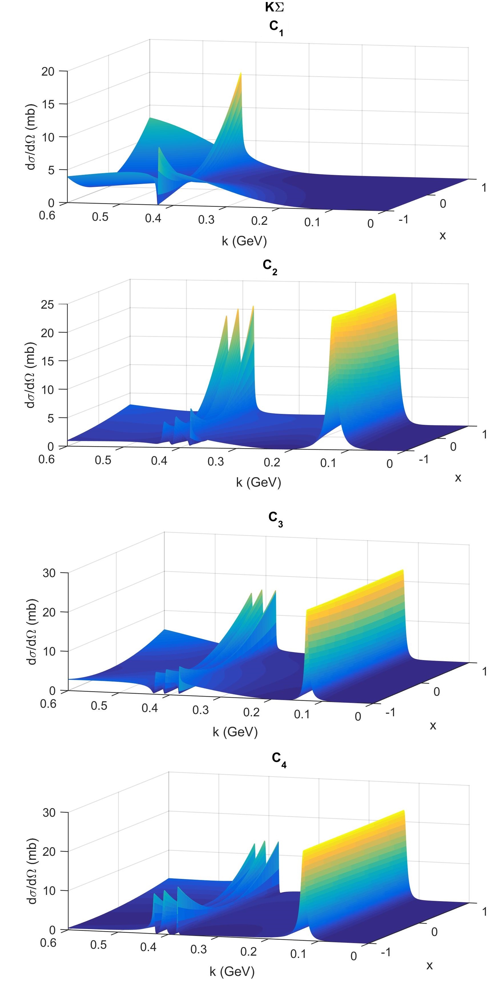
Figure 6: Angular Distribution in the $K\Sigma$ scattering

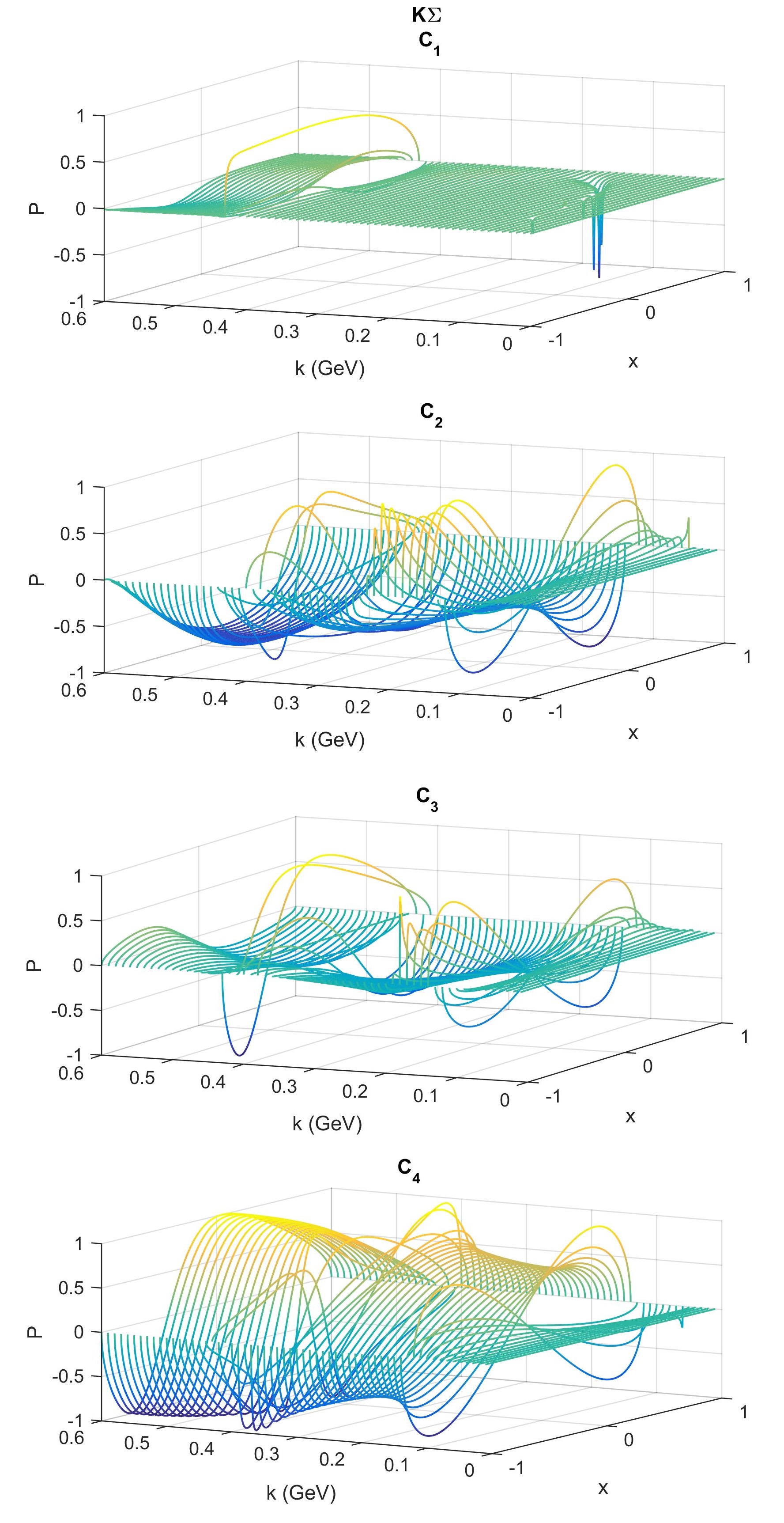
Figure 7: Polarization in the $K\Sigma$ scattering

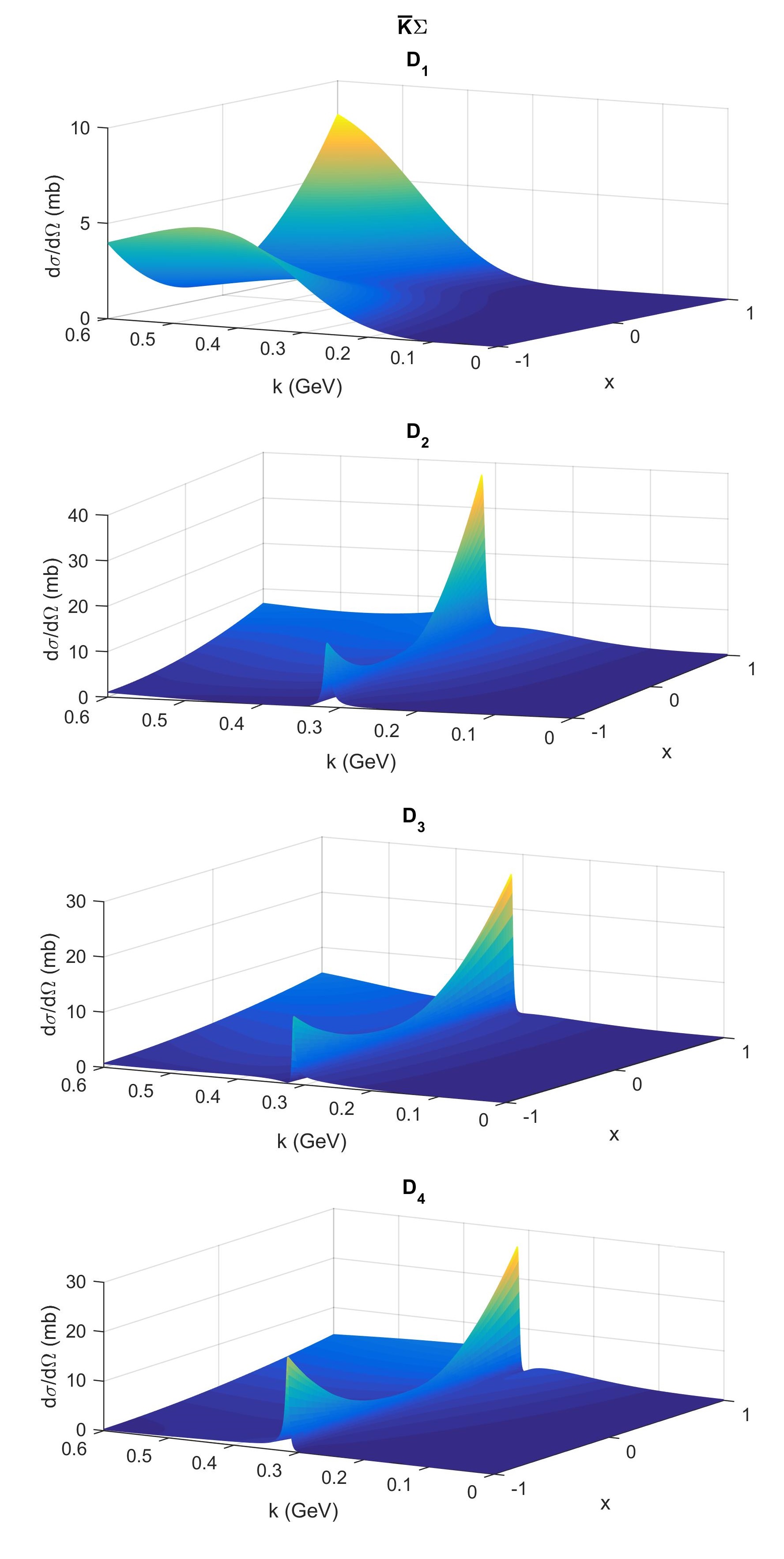
Figure 8: Angular Distribution in the $\overline{K}\Sigma$ scattering

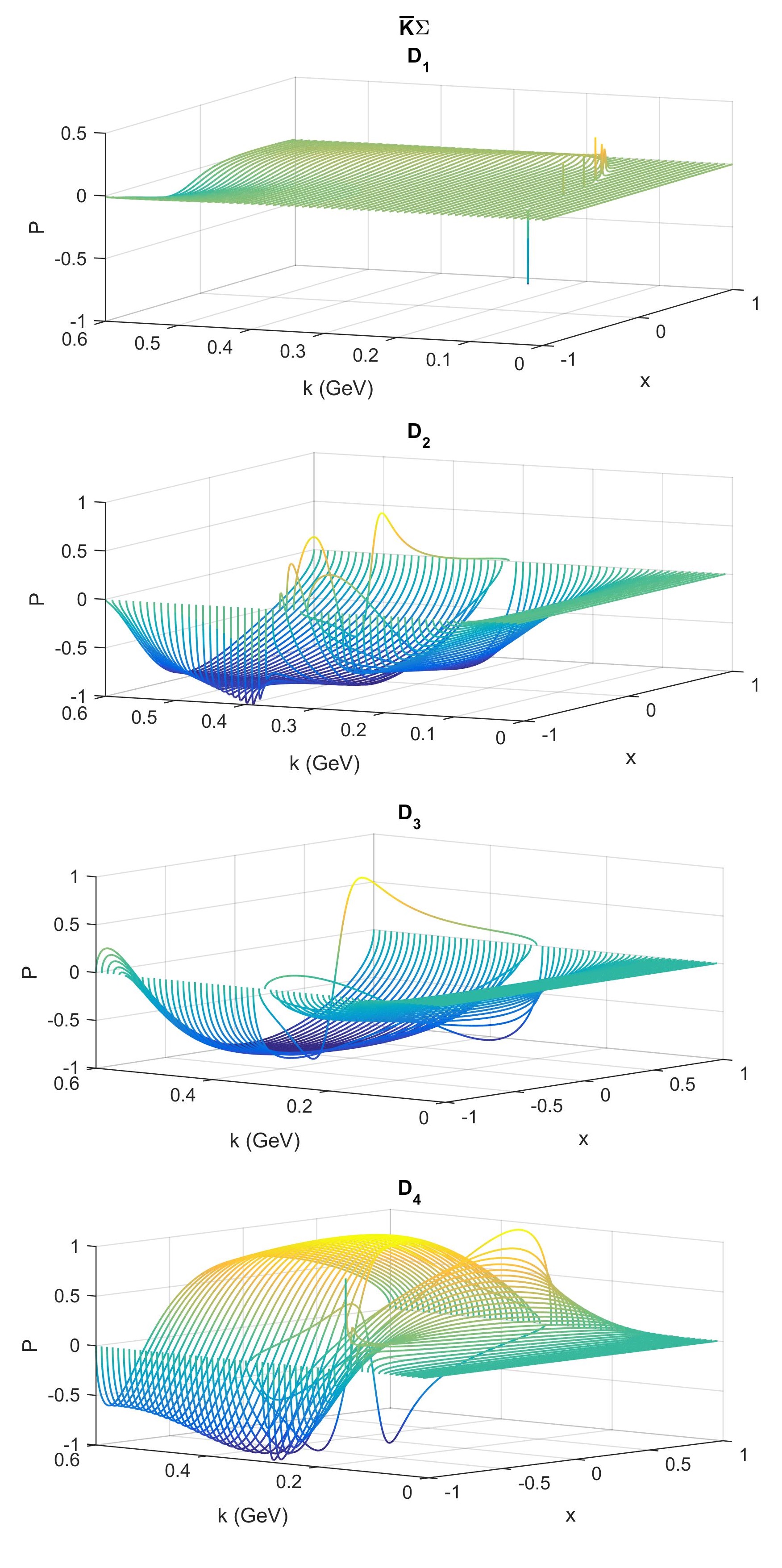
Figure 9: Polarization in the $\overline{K}\Sigma$ scattering

V Discussion

In this paper we have calculated the angular distributions and polarizations for many reactions considering kaon-hyperon and antikaon hyperon interactions. We have considered a model based in effective nonlinear chiral lagrangians, previously used to describe the pion-hyperon BH and pion-nucleon manc interactions.

As we pointed before, an important aspect is that at low energies the resonances play an important role in the cross sections. The polarizations in general are oscillating functions, that may be small, as it can be seen in the reactions labeled by $C_{1}$ and $D_{1}$ (Fig. 7 and Fig. 9), but also may be consistenly large, as for example in the reactions represented by $D_{4}$ shown in Fig. 9.

Despite the fact that this kind of reactions are very important in order to understand the basic proprieties of the hyperon physics, we imagine that, maybe due to technical difficulties, in a near fucture this kind of observable will not be measured experimentally. A possible way to determine some phase-shifts is a procedure similar to the one used in the HyperCP experiment hyper1 , hyper2 , where $\delta_{S}-\delta_{P}$ has been determined for the $\pi\Lambda$ interaction observing the production and decay of the $\Xi$ hyperon in high energy experiments. The results presented in BH are in good accord with these data, and then validate the model proposed in the study of the meson-hyperon interactions. We expect that this kind of question motivates future experiments.

Although, as it has been said before, the main motivation for this work is the polarization of hyperon produced in high energy collisions. As it has been shown in cy -ccb2 , the low energy meson-hyperon interactions are key elements, as far as the produced hyperons interact with the surrounding medium before the detection, and these interactions may affect the final hyperon polarization. In cy -ccb2 , only the pion-hyperon interactions have been considered and this fact motivated this work. So, a natural improvement of the model is the inclusion of the kaon-hyperon interactions. Observing the polarization results in Fig.5-9 we may conclude that they can have some effect in high energy processes if the final-state interactions are considered, and these corrections may be interpreted as experimental verifications of the results presented in this work. These calculations will be shown in future works.

VI Acknowledgments

This study has been partially supported by the Coordenação de Aperfeiçoamento de Pessoal de Nível Superior (CAPES) – Finance Code 001.

VII Appendix

Considering a process where $p$ and $p^{\prime}$ are the initial and final hyperon four-momenta, $k$ and $k^{\prime}$ are the initial and final meson four-momenta, the Mandelstam variables are given by

$$s = (p+k)^{2}=(p^{\prime}+k^{\prime})^{2}=m^{2}+m_{K}^{2}+2Ek_{0}-2\vec{k}.\vec{p}\ ,$$

$$u = (p^{\prime}-k)^{2}=(p-k^{\prime})^{2}=m^{2}+m_{K}^{2}-2Ek_{0}-2\vec{k}^{\prime}.\vec{p}\ ,$$

$$t = (p-p^{\prime})^{2}=(k-k^{\prime})^{2}=2(\vec{k})^{2}x-2(\vec{k})^{2}\ .$$

In the center-of-mass frame, the energies will be defined as

$$k_{0}=k^{\prime}_{0}=\sqrt{|\vec{k}|^{2}+m_{K}^{2}}$$

$$E=E^{\prime}=\sqrt{|\vec{k}|^{2}+m^{2}}$$

where $m$ and $m_{K}$ are the hyperon mass and the kaon mass, respectively.

We also define the variable

$$x=\cos\theta$$

where $\theta$ is the scattering angle. For the energy and for the 3-momentum of the intermediary particles we have the relations

$$(E_{B^{*}}\pm m_{\Lambda})=\frac{(m_{B^{*}}\pm m_{\Lambda})^{2}-m_{K}^{2}}{2m_{B^{*}}}\ ,$$

$$(\vec{q}_{B^{*}})^{2}=E_{B^{*}}^{2}-m_{\Lambda}^{2}=(E_{B^{*}}+m_{\Lambda})(E_{B^{*}}-m_{\Lambda})\ .$$

where $E_{B^{*}}$ and $\vec{q}_{B^{*}}$ are the energy and the momentum of the intermediary baryon $B^{*}$ in the center-of-mass frame, respectively.

References

• (1) G. Bunce et al., Phys. Rev. Lett. 36, 1113 (1976).
• (2) K. Heller et al., Phys. Lett. 68B 480 (1977); K. Heller et al., Phys. Rev. Lett. 41 607 (1978); S. Erhan et al., Phys. Lett. 82B 301 (1979).
• (3) B. Lundberg et al., Phys.Rev. D 40, 3557 (1989).
• (4) C. Wilkinson et al., Phys. Rev. Lett. 46 803 (1981).
• (5) L. Deck et al., Phys. Rev. D 28, 1 (1983).
• (6) R. Ramerika et al., Phys. Rev. D 33, 3172 (1986).
• (7) M. I. Adamovich et al., Z. Phys. A 350, 379 (1995).
• (8) P. M. Ho et al., Phys. Rev. Lett. 65, 1713 (1990); P. M. Ho et al., Phys. Rev. D 44, 3402 (1991).
• (9) A. Morelos et al., Phys. Rev. Lett. 71, 2172 (1993); A. Morelos et al., Phys. Rev. D 52, 3777 (1995).
• (10) STAR Collab., B. I. Abelev et al., Phys. Rev. C, 76, (2007) 024915.
• (11) STAR Collab, L. Adamczyk et al., Nature 548, 62 (2017).
• (12) B. Andersson, G. Gustafson and G. Ingelman, Phys. Lett. 85B, 417 (1979).
• (13) T.A. DeGrand and H.I. Miettinen, Phys. Rev. D 24, 2419 (1981).
• (14) J. Soffer and N.A. Törnqvist, Phys. Rev. Lett. 68, 907 (1992).
• (15) S.M. Troshin and N.E. Tyurin, Phys. Rev. D 55, 1265 (1997).
• (16) STAR Collab, L. Adam et al., arXiv: 1905.11917 (2019).
• (17) STAR Collab, I. Upsal et al., J. Phys. Conf. Ser. 736 (2016), no.1, 012016.
• (18) I. Karpenko and F. Becattini, Eur. Phys. J. C77 (2017), no.4 2013.
• (19) F. Becattini, I. Karpenko, M. Lisa, I. Upsal and S. Voloshin, Phys. Rev. C95 (2017), no.5, 054902.
• (20) V. P. Ladygin, A. P. Jerusalimov and N. B. Ladygina, Phys. Part. Nucl. Lett. 7 (2010), 349.
• (21) Y. Xie, D. Wang, L. P. Csernai, Phys. Rev. C95 (2017), no.3, 031901.
• (22) D. Montenegro, L. Tinti and G. Torrieri, Phys. Rev. D96 (2017), no.5, 056012.
• (23) B. Betz, M. Gyulassi and G. Torrieri, Phys. Rev. C76 (2007), 044901.
• (24) L. M. G. Martin et al. Eur. Phys. J. C (2019) 79:634.
• (25) R. S. Hayano et al. Phys. Lett. B 231, 355 (1989).
• (26) T. Nagae et al. Phys. Rev. Lett. 80, 1605 (1998).
• (27) S. Bart et al. Phys. Rev. Lett. 83, 5238 (1999).
• (28) A. Armat and H. Hassanabadi, Can. J. Phys. 94 (2016), no.4, 365.
• (29) J. Schaffner, C. Greiner and H. Stöcker, Phys. Rev. C 46, 322 (1992).
• (30) N. K. Glendenning, Astrophys. J. 293, 470 (1985).
• (31) J. Schaffner-Bielich, Nucl. Phys. A 804, 309 (2008).
• (32) M. Baldo, G. F. Burgio and H. J. Schulze, Phys. Rev. C 61 055801 (2000).
• (33) I. Vidana, A. Polls, A. Ramos, L. Engvik and M. Hjorth-Jensen, Phys. Rev. C 62, 035801 (2000).
• (34) C. C. Barros Jr. and Y. Hama, Int. J. Mod. Phys. E 17 371 (2008).
• (35) C. C. Barros Jr. and Y. Hama, Phys. Lett. B 699, 74 (2011).
• (36) C. C. Barros Jr., J. Phys. Conf. Ser. 509, 012056 (2014).
• (37) M. G. L. N. Santos, C. C. Barros Jr., Phys. Rev. C 99, 025206 (2019).
• (38) H. T. Coelho, T. K. Das and M. R. Robilotta, Phys. Rev. C 28, 1812 (1983).
• (39) C. C. Barros and Y. Hama, Phys. Rev. C 63, 065203 (2001).
• (40) C. C. Barros Jr. and M. R. Robilotta, Eur. Phys. J. C 45, 445 (2006).
• (41) C. C. Barros Jr., Phys. Rev. D 68, 034006 (2003).
• (42) C. Patrignani, et al., Chin. Phys. C 40, 100001 (2016).
• (43) H. Pilkuhn, The Interaction of Hadrons, (North-Holland, Amsterdam, 1967).
• (44) E. T. Osypowski, Nucl. Phys. B 21, 615 (1970).
• (45) M. G. Olsson and E. T. Osypowski, Nucl. Phys. B 101, 136 (1975).
• (46) J. Gasser, M. E. Sainio and A. Švarc, Nucl. Phys. B 307, 779 (1988); T. Becher and H. Leutwyler, Eur. Phys. Journal C 9, 643 (1999); JHEP 106, 17 (2001).
• (47) J. Gasser, H. Leutwyler and M. E. Sainio, Phys. Lett. B 253, 252 (1991); 253, 260 (1991).
• (48) A. I. L’vov, S. Scherer, B. Pasquini, C. Unkmeir and D. Drechsel, Phys. Rev. C 64, 015203 (2001).
• (49) M. R. Robilotta, Phys. Rev. C 63, 044004 (2001).
• (50) V. Stoks, T. A. Rijken, Nuclear Physics A, Elsevier, v. 613, n. 4, p. 311–341, (1997).
• (51) J. D. Swart, Reviews of Modern Physics, APS, v. 35, n. 4, p. 916, (1963).
• (52) A. Chakravorty et al., Phys. Rev. Lett. 91, 031601 (2003).
• (53) M. Huang et al., Phys. Rev. Lett. 93, 011802 (2004).