Disaster Resilience and Asset Prices††thanks: Marco Pagano gratefully acknowledges financial support from the Italian Ministry for Education, University and Research (MIUR) and the Einaudi Institute for Economics and Finance (EIEF). Christian Wagner is an associate member of the Center for Financial Frictions (FRIC) and acknowledges support from grant no. DNRF102. Pagano: pagano56@gmail.com. Wagner: christian.wagner@wu.ac.at. Zechner: josef.zechner@wu.ac.at
Abstract
This paper investigates whether security markets price the effect of social distancing on firms’ operations. We document that firms that are more resilient to social distancing significantly outperformed those with lower resilience during the COVID-19 outbreak, even after controlling for the standard risk factors. Similar cross-sectional return differentials already emerged before the COVID-19 crisis: the 2014-19 cumulative return differential between more and less resilient firms is of similar size as during the outbreak, suggesting growing awareness of pandemic risk well in advance of its materialization. Finally, we use stock option prices to infer the market’s return expectations after the onset of the pandemic: even at a two-year horizon, stocks of more pandemic-resilient firms are expected to yield significantly lower returns than less resilient ones, reflecting their lower exposure to disaster risk. Hence, going forward, markets appear to price exposure to a new risk factor, namely, pandemic risk.
JEL classification: G01, G11, G12, G13, G14, Q51, Q54.
Keywords: asset pricing, rare disasters, social distance, resilience, pandemics.
1 Introduction
The COVID-19 pandemic and the resulting lockdown are currently inflicting massive harm on the economy, in the form of unprecedented output losses, massive redundancies and countless bankruptcies. The effects of the pandemic are widely perceived not to be purely transient, as witnessed by current changes in expectations (Coibion et al., 2020b; Hanspal et al., 2020; Coibion et al., 2020a) and in asset prices (Gormsen and Koijen, 2020). But its effects are also proving to be quite heterogeneous: some firms, especially in high-tech industries, appear to have adapted quite well to social distancing requirements, for instance by resorting extensively to teleworking, while others, such as food catering, travel and tourism, could not do so, as the nature of their business requires close contact with customers and/or among employees. This heterogeneity is also visible in the diverging stock price performance of companies: in the first quarter of 2020, stocks such as Apple, Microsoft and Google outperformed the market, yielding market-adjusted returns of 19%, 12% and 33% respectively, while others such as Marriott, United Airlines and Royal Caribbean massively underperformed, with market-adjusted returns of , and .
Hence, the COVID-19 shock has unearthed a hitherto hidden economic watershed, namely, that between disaster-resilient activities and non-resilient ones. Insofar as the COVID-19 pandemic persists or revives in the near future, or similar disasters may occur further in the future, resilience may become a key firm attribute, one which will be relevant to investors’ portfolio choices, banks’ lending policies, and managers’ investment decisions.
In this paper, we investigate whether asset prices reveal growing investors’ awareness that pandemic resilience, defined as reliance on technologies and/or organizational structures that are robust to social distancing, is priced by security markets. To measure firms’ resilience to pandemics, we rely on measures recently introduced in labor economics by Dingel and Neiman (2020), Hensvik et al. (2020) and Koren and Pető (2020), intended to capture the extent to which firms’ operations are compatible with social distancing. These measures quantify the degree to which jobs can be done from home and do not rely on human interaction in physical proximity.
We then test whether the stocks of more resilient companies have generated excess returns, after controlling for market risk and other established risk factors, before and/or during the COVID-19 shock. We find this to be the case: pandemic-resilient stocks outperformed less resilient ones not only between late February and March 2020, i.e. during the outbreak of the pandemic, but also in the previous six years, in which their cumulative excess return was of similar magnitude as during the crisis.
Furthermore, we investigate the returns that investors expect the two stock classes to generate after the COVID-19 shock, by extracting the expected stock returns implied by option prices. We find that, going forward, pandemic-resilient stocks are expected to generate lower excess returns, indicating that, since the COVID-19 pandemic materialized, the market has priced a disaster premium.
Thus, our research question is not only whether, but also when financial markets started pricing disaster risk and resilience to it. Interestingly, our evidence indicates that investors became gradually aware of such risk even before the COVID-19 shock, and they consider such risk to be still price-relevant, even after it has materialized.
Given the largely unanticipated nature of the current pandemic, it may appear unrealistic that investors became cognizant to its threat in advance. But it should be recalled that as early as five years before the COVID-19 outbreak, high-profile business and political leaders already issued public warnings of the risk of devastating epidemics. For instance, in a speech delivered on 2 December 2014 at the NIH about the response to the Ebola epidemic, U.S. President Barack Obama stated:
“There may and likely will come a time in which we have both an airborne disease that is deadly. And in order for us to deal with that effectively, we have to put in place an infrastructure – not just here at home, but globally – that allows us to see it quickly, isolate it quickly, respond to it quickly. […] So that if and when a new strain of flu, like the Spanish flu, crops up five years from now or a decade from now, we’ve made the investment and we’re further along to be able to catch it. It is a smart investment for us to make. It’s not just insurance; it is knowing that down the road we’re going to continue to have problems like this – particularly in a globalized world where you move from one side of the world to the other in a day.”
Similarly, in 2015, Microsoft co-founder Bill Gates gave a TED Talk about pandemics that attracted widespread attention. In this talk he warned that in 2014 the world had barely avoided a global outbreak of Ebola, largely because of pure luck, and, just like Obama, alerted the audience to the need to prepare for future pandemics, from scenario planning to vaccine research and health worker training. Hence, it cannot be ruled out that the most alert investors may have started taking into account such concerns in their portfolio choices well in advance of the current pandemic, shying away from the stocks of companies that would be less resilient to it and starting to overweight those likely to be more resilient.
One may also wonder why even after the occurrence of COVID-19 the market still prices pandemic risk to some extent, being willing to accept lower expected returns on more resilient stocks, as revealed by option prices according to our estimates. However, currently there is still high uncertainty regarding the duration of the COVID-19 pandemic. Medical experts have repeatedly warned about the risk of a second wave of contagion as the lockdown measures are gradually relaxed (see Xu and Li, 2020, among others). Indeed, top health officials do not rule out that the disease may become endemic. On 13 May 2020, Dr. Mike Ryan, executive director of emergencies at the World Health Organization (WHO) stated:
“I think it’s important to put this on the table. This virus may become just another endemic virus in our communities. And this virus may never go away. HIV has not gone away, we’ve come to terms with the virus […] I think it is important that we’re realistic and I don’t think anyone can predict when or if this disease will disappear.”
Such uncertainty, possibly coupled with heightened awareness that similar disasters may occur again in the future, could explain why, since COVID-19, pandemic risk is priced in the cross-section of returns, as shown by our evidence based on option prices. Hence, going forward, asset pricing models will have to include exposures to this additional risk factor among those used to explain the cross-section of returns, and asset managers will have to take such exposures into account in portfolio selection.
Our analysis is related to the asset pricing literature on rare disasters, starting with Rietz (1988), who extends the Lucas (1978) model to include a rare disaster state and shows that this leads to high equity risk premia and low risk-free returns, even with reasonable time discounting and risk preferences. Barro (2006) and Barro (2009) extend this model and show that empirically calibrated disaster probabilities may suffice to explain the observed high equity premium, low risk-free rate and stock return volatility. The theoretical literature on disaster risk has also been extended to allow for learning (see, e.g.,Veronesi (2004), Wachter and Zhu (2019), Gillman et al. (2014), Lu and Siemer (2016)), and/or for stochastic disaster risk (see, e.g., Wachter (2013) and Gabaix (2012)).
One common feature of these models is that risk premia that would appear abnormally high conditioning on no disaster occurring, are in fact justified, being merely an equilibrium compensation for the expected loss in a disaster plus a risk premium as this loss occurs when the marginal utility of consumption is high. In particular, the model by Gabaix (2012) implies that, in the cross-section of stocks, those that are expected to be less resilient to disasters, should carry a higher risk premium, conditioning on no disaster occurring, but also unconditionally. Our empirical analysis speaks to these predictions.
Our work is also related to a fast growing literature on the stock market response to the COVID-19 pandemic in the first quarter of 2020. The early comprehensive study by Ramelli and Wagner (2020) documents that during the ‘outbreak’ period (which they define as 20 January to 21 February 2020), U.S. firms with high exposure to China and, more generally, to international trade, as well as firms with high leverage and low cash holdings experienced the sharpest stock price declines. The leverage- and cash holding effects also persist through the ‘fever’ period (from 24 February to 20 March 2020). Bretscher et al. (2020) provide evidence for supply chain effects in the cross-section of stocks during COVID-19. Moreover, Albuquerque et al. (2020) find that firms with high environmental and social (ES) ratings offered comparably higher returns and lower return volatility in the first quarter of 2020.
Some studies relate the price response of different stocks to the pandemic to the corresponding firms’ exposure to the disease. Ramelli and Wagner (2020) and Hassan et al. (2020) analyze conference call data, which the latter use to construct text-based, firm-level measures for exposures to epidemic diseases, and find that stock returns are significantly and negatively related to disease exposures, with demand- and supply-chain related concerns being primary drivers. Alfaro et al. (2020) analyse the effect of unanticipated changes in infections during the SARS and the COVID-19 epidemics on stock returns, and show that stock prices drop in response to high unexpected infections. In the cross-section, exposure to pandemic risk turns out to be greater for larger and more capital intensive firms, and, consistently with Ramelli and Wagner (2020), more levered and less profitable ones.
Some of the results obtained for the response of U.S. stock returns to the pandemic appear to extend to non-U.S. stock returns. Ding et al. (2020) show for a sample of over 50 countries that firms with better financials, less supply chain exposures and more corporate social responsibility (CSR) activities experienced milder stock price reactions in the first quarter of 2020. Other studies focus on the response of country-level stock market indices to COVID-19: Ru et al. (2020) find that stock markets in countries with 2003 SARS experience reacted more quickly to the outbreak than countries without prior experience, while Gerding et al. (2020) document that market declines were more severe in countries with lower fiscal capacity, defined as higher debt/GDP ratio. Finally, Croce et al. (2020) use Twitter news to study the (real-time) COVID-19 caused contagion in global equity markets.
Our analysis differs from that in all these papers since it focuses on the asset pricing implications of companies’ exposure to social distancing, which is the main economic consequence of the epidemic, and studies such implications not only for the period of the COVID-19 outbreak, but also prior and after its occurrence. This enables us to investigate whether learning about pandemic risk occurred in advance of the outbreak, and whether investors kept pricing it since the outbreak.
The rest of the paper is structured as follows. Section 2 provides a framework to interpret the relationship between disaster risk and the stock returns of firms featuring different disaster resilience. Section 3 provides a brief discussion of alternative measures of firms’ disaster resilience. The data and results are presented in Section 4. Section 5 concludes.
2 Disaster Awareness and Risk Premia
In this section we sketch three distinct and mutually exclusive models of how financial markets may respond to disaster risk and to its materialization. As we shall see, each model has different predictions about the stock return differential of resilient vs. non-resilient firms prior, during and after the occurrence of a disaster, as shown in Table 1. Our empirical analysis in Section 4 will investigate which of the three sets of predictions is most consistent with the data.
| Theory | Before COVID-19 | During COVID-19 | After COVID-19 |
|---|---|---|---|
| Unpriced disaster risk | Zero | Positive | Zero |
| Priced disaster risk | Negative | Positive | Negative |
| Pre-disaster learning | Positive | Positive | Negative |
Unpriced disaster risk. We start with a model where disaster is completely unexpected. In the case of COVID-19, this amounts to assuming that before the first quarter of 2020 financial market participants were unaware of the danger posed by the virus and of its consequences in terms of social distancing. Going forward, a new disaster is again regarded as a zero-probability event, or anyway as being price irrelevant (for instance, in the case of COVID-19, due to development of vaccines and/or effective drugs). In this model, disaster risk would not be priced before COVID-19 nor after it. Such market expectations could result either from bounded rationality, i.e. investors assigning a zero probability weight to a positive probability event, or from a disaster truly having a negligible probability both before and after its occurrence. In the latter case, unpriced disaster risk would be consistent with rational expectations.
If this is the correct model in the case of the COVID-19 pandemic, one should observe (i) no return pattern related to firm pandemic resilience prior to 2020; (ii) a sharper price drop for less resilient firms than for more resilient ones at the time of the outbreak, as investors take into account that the cash flows of the former will be hurt more than those of the latter; (iii) no differential response of the expected returns of the two classes of firms after the crisis, since COVID-19 does not lead to any updating of the return-generating process, i.e. disaster risk remains unpriced. As disaster is considered as a one-time event, its occurrence leaves the stochastic discount factors of all stocks unchanged.
Priced disaster risk. The second model is one where disasters, however rare, are rationally anticipated, so that more resilient firms are priced at a premium relative to less resilient ones, i.e. offer a lower expected return in no-disaster periods, as predicted by Barro (2006), Barro (2009) and Gabaix (2012). Such models predict that, in equilibrium, securities more exposed to a disaster, i.e. those issued by less resilient firms, pay a risk premium to compensate investors for this risk. Hence, they predict that (i) prior to the disaster, stocks’ excess returns are related to firms’ disaster resilience; (ii) during the disaster, investors take into account that the cash flows of less resilient firms drop by more than those of the more resilient ones, so that their disaster-time stock performance is worse; (iii) after the disaster, the pre-disaster excess return pattern re-emerges, i.e. disaster risk remains priced. In principle, this hypothesis does not preclude that investors may update the probability of disasters upon the occurrence of one: if they have increased this probability as a result of COVID-19, the expected return differential between non-resilient and resilient firms should become more pronounced after the pandemics than it was before it.
Prior learning about disaster risk. Finally, we consider a model where investors learn about the probability of a disaster occurring or about its implications before its occurrence. In the case of COVID-19, as mentioned in the introduction, they may have revised upwards the probability of a pandemic occurring or become more keenly aware of its social distancing implications, for instance as a result of SARS, Ebola, and/or the statements by Bill Gates, Barack Obama and other opinion leaders. By the same token, investors may have become more aware of the characteristics that make firms more resilient to pandemics. Any of these forms of learning implies a demand shift by investors from less to more resilient stocks before the pandemic, leading the latter to outperform the former, once their respective exposures to “traditional” risk factors are controlled for. Once disaster strikes, one would again observe the stocks of more resilient firms outperforming less resilient ones. But this pattern should reverse in the post-disaster phase: as at that stage learning would be complete, the stocks of more resilient firms will be priced at a premium relative to less resilient ones, i.e. should offer a lower expected return. This scenario has parallels with learning about the “importance” of Environmental, Social and Governance (ESG) scores by investors. In a rational expectations equilibrium without learning, portfolios with strict ESG rules should underperform, but in the presence of gradual learning about the importance of ESG ratings for investors, the stocks of firms with high ESG ratings appreciate, and ESG mutual funds outperform (see Pastor et al., 2020).
Hence, this model predicts that (i) excess returns of resilient relative to non-resilient firms should be observed prior to the disaster; (ii) when disaster strikes, investors take into account that the cash flows of less resilient firms drop by more than those of more resilient ones; (iii) after the disaster, resilient firms offer lower expected returns that non-resilient ones, as learning about disaster risk has taken place.
3 Measuring Firm Resilience to Pandemics
This section describes social distancing measures that may be relevant for the pricing of stocks, as firms with operations requiring less direct physical interaction and more easily performed from home should be more resilient to social distancing rules than other firms. To gauge the effect of social distancing on firms, recent research in labor economics has developed measures of the extent to which jobs can be done from home and rely on human interaction in physical proximity. Some studies have developed such measures starting from worker-level survey responses, while others have done so by characterizing the tasks required by each occupation based on the Occupational Information Network (O*Net) and on the authors’ own judgement.
Hensvik et al. (2020, HLR) use the first approach: they rely on the ‘American Time Use Survey’ (2011-2018) to estimate the prevalence of working at ‘home’ and at the ‘workplace’ and, starting from worker-level survey responses, estimate the fraction of employees that work at home and at the workplace, as well as the hours worked at home and at the workplace at the industry-level.111As the authors mention, their measures for working at home should provide a lower bound for the current situation, as the COVID-19 crisis is likely to have prompted additional substitution of work at the workplace with work at home. Instead, both Dingel and Neiman (2020, DN) and Koren and Pető (2020, KP) use data from O*Net surveys. DN use this data, and their own judgement, to assess the teleworkability of occupations and provide industry-level estimates for the percentage of jobs that can be done at home as well as for the percentage of wages associated with teleworkable occupations. KP construct three types of industry-level measures of face-to-face interactions, depending on whether these are due to internal communication (‘teamwork’), external communication (‘customers’), or physical proximity to others (‘presence’). They also aggregate ‘teamwork’ and ‘customers’ to a measure of ‘communication’ intensity and construct an industry-level measure of the percentage of employees ‘affected’ by social distancing regulations due to their occupations being communication-intensive and/or requiring close physical proximity to others.222The estimates of these studies are available for NAICS industry classifications, at the 2- and 3-digit level for DN, at the 4-digit level for HLR, and at the 3-digit-level for KP. For details on the data, see Table A.1 in the Appendix.
In our estimates, we rely primarily on the measures proposed by KP, but also check whether our results are robust to the use of those produced by HLR and DN. The results presented in the next section focus mostly on KP’s ‘affected_share’ variable. We choose this as our main variable because, beside teleworkability, it also explicitly accounts for physical proximity to others, i.e. exactly what social distancing rules aim to avoid. Additionally, we consider DN’s measure of the fraction of wages accounted for by jobs that can be performed at home (‘teleworkable_manual_wage’) and HLR’s measure of daily work hours at the workplace (‘dur_workplace’). However, we also discuss results obtained using all other variables suggested by KP, DN, and HLR. Table A.1 in the Appendix lists all the measures and presents their definitions.
4 Empirical Results
We use the NAICS industry classification of stocks to assign the DN, HLR, and KP metrics to firms, and code each firm as a ‘High’ or ‘Low’ resilience one, depending on how its industry scores relative to the median value of the relevant metric. Then, we analyze whether and how the resulting variation in U.S. firms’ pandemic resilience affects the cross-section of their stock returns at the time of the COVID-19 shock (Subsection 4.2), before the shock (Subsection 4.3) and after its occurrence (Subsection 4.4).
4.1 Data and Methodology
We obtain prices for all common stocks listed at the NYSE, AMEX and NASDAQ from the Compustat Capital IQ North America Daily database and compute daily returns, accounting for price-adjustments and dividends. We also retrieve data on daily risk-free, market and standard factor returns from Kenneth French’s website. Our estimates in Subsection 4.2 require daily data from January 2019 to March 2020: after estimating firms’ exposures to common factors from 2019 data, we use these exposures to compute factor model-adjusted stock returns in the first quarter of 2020.333This approach follows Ramelli and Wagner (2020) and other related papers.
For the regressions of daily stock returns on factor returns, we require a minimum of 127 daily observations, and estimate the following specifications: we alternatively regress stock returns on market excess returns (CAPM), on the returns of the three Fama and French (1993) factors (FF3, i.e. market, size, and value) and the five Fama and French (2015) factors (FF5, i.e. market, size, value, investment, and profitability). In addition, we augment the FF3 and FF5 specifications by the momentum factor (Carhart, 1997) so as to obtain FF4 and FF6 exposures. The 2019 exposures are then used to measure factor model-adjusted stock returns in the first quarter of 2020 as the difference between a stock’s daily excess return and its CAPM beta multiplied by the daily market excess return; we proceed analogously for the FF specifications.
Next, stock return data are matched with the resilience proxies based on KP, DN, and HLR metrics by industry, based on firms’ 2-, 3-, or 4-digit NAICS codes. Only industries for which resilience measures are available are retained in the data set. Moreover, firms with equity market capitalization below USD 10 million are dropped from the sample. For the first quarter of 2020, this results in a sample with a total of 227,812 observations for 3,614 firms in 75 industries at the NAICS 3-digit level for KP and DN, and 222 industries at the NAICS 4-digit level for HLR.
For the analysis in Subsection 4.4, we additionally obtain S&P 500 index option and individual stock options data from OptionMetrics for the first quarter of 2020. We use the volatility surface data to compute -measures of the risk-neutral variance, keeping data for firms for which we can compute -measures for horizons of 30, 91, 182, 365, and 730 days, and match this with the stock data. This results in a sample of 160,951 observations for 2,721 firms in 74 industries at the NAICS 3-digit level for KP and DN and 212 industries at the NAICS 4-digit level for HLR.
4.2 Returns and Firm Resilience during the Disaster
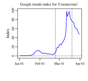
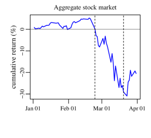
We study stock returns in the first quarter of 2020, and specifically from February 24, the day after Italy introduced its lockdown, to March 20, the last trading day before the Fed announced aggressive action intended to soften the blow of the pandemic.444This period corresponds to the ‘fever’-period in Ramelli and Wagner (2020); see their paper for a detailed account of the sequence of events. On Monday March 23, the Fed unveiled its plan to buy an unlimited amount of bonds with government guarantees, including some commercial mortgage debt. It also established the Secondary Market Corporate Credit Facility (SMCCF), in order to purchase existing investment-grade corporate debt, including exchange-traded funds, as well as the Primary Market Corporate Credit Facility (PMCCF), to purchase newly issued corporate bonds, so as to prevent companies facing pandemic fallout from dismissing employees and terminating business relationships. As shown by Panel A of Figure 1, in this time window there was a surge in the public’s attention to the COVID-19 epidemic (as measured by Google trends), while the prices of U.S. stocks (as measured by the Fama-French market factor) fell sharply.
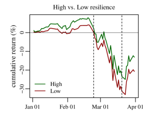
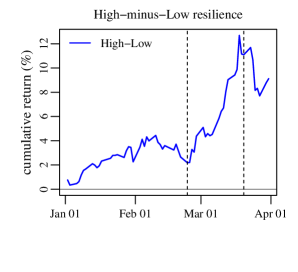
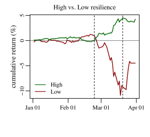
A first look at the data suggests that the stocks of more pandemic-resilient firms, i.e. those included in the ‘High’ resilience portfolio (based on the ‘affected_share’ metric by KP) performed better in this time window than those in the ‘Low’ resilience portfolio. Panel B in Figure 1, which plots cumulative excess returns for the value-weighted portfolios of firms with high and low resilience, shows that both portfolios dropped sharply in price, but that of high-resilience firms depreciated far less: from February 24 to March 20, their shares outperformed those of the other group by approximately 10%.
[Insert Figure 1]
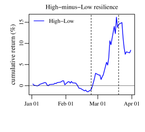
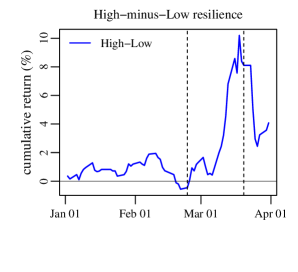
Since the different performances of the two portfolios shown in Figure 1 may stem from their different exposure to standard risk factors, we estimate CAPM- and FF-exposures from daily data in 2019. We then use these exposures to compute daily CAPM-adjusted and FF-adjusted returns, i.e., excess returns net of such exposures multiplied by the respective factor returns (see Subsection 4.1 for details). Figure 2 presents the results: controlling for market factor risk (CAPM-adjusted returns in Panel A), the cumulative return of the High- and Low-resilience portfolio are about +10% and 15%, respectively, from February 24 to March 20, i.e. the cumulative CAPM-adjusted High-minus-Low return is approximately 25%. Panels B and C show that accounting for the FF-factors does not change the results qualitatively: the resulting risk-adjusted return differentials are in the range between 15% and 20%. The plots suggest that the differential return between the two portfolios has been negligible from early January until late February, and that the results in the COVID-19 time window are mostly driven by the sharp decline of the Low-resilience portfolio. Once the Fed announced its intervention (on March 23) the High-resilience portfolio recovered slightly and, as a result, the Low-minus-High differential dropped. Interestingly, the time-series of the cumulative Low-minus-High returns resembles that of the Google trends index. Indeed, regressing daily returns on changes in the Google index confirms a statistically significant relation, with between 0.19 and 0.22, depending on which factor-model adjustment is used.
[Insert Figure 2]
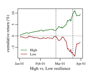
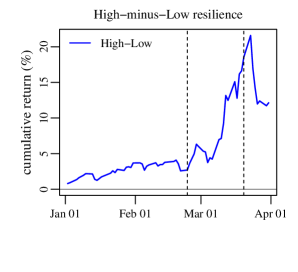
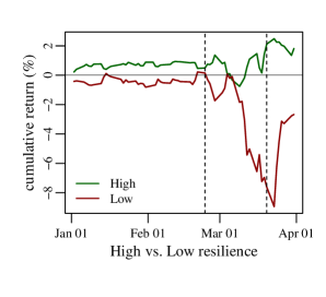
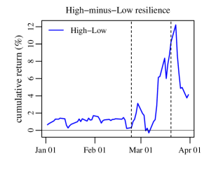
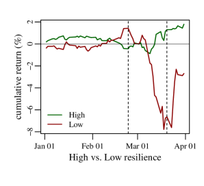
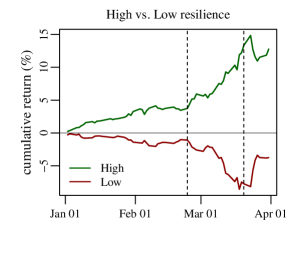
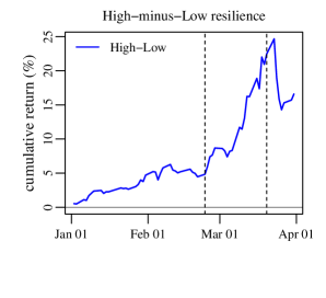
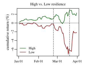
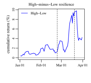
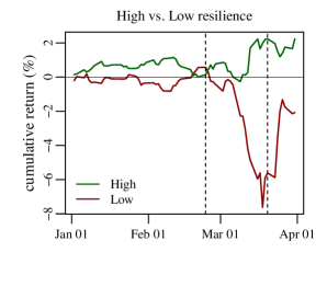
Figures A.1 and A.2 in the Appendix provide evidence on the robustness of the results shown in Figure 2 with respect to other resilience measures. They plot the risk-adjusted returns and the differentials of the High- and Low-resilience portfolios based on DN’s ‘teleworkable_manual_wage’ and HLR’s ‘dur_workplace’. The results are qualitatively similar to those in Figure 2.
To analyze the statistical significance of these findings, Table 2 reports the averages of daily excess returns (in Column 1) and risk-adjusted returns (in Columns 2 to 6) for High-resilience and Low-resilience stocks from February 24 to March 20, as well as the difference between the two, using the resilience measures based on KP, DN and HLR. Panel A shows that the differential return based on SKP’s ‘affected_share’ metric is statistically significant, whether it is based on raw excess returns or adjusted for market exposure (CAPM), for the classic Fama-French factors (FF3 and FF5) or for those that also control for momentum (FF4 and FF6). For resilience measures based on DN (Panel B) and HLR (Panel C), the average CAPM-adjusted differential returns are statistically significant as well, but there is some variation in the significance of the FF-adjusted returns. A common feature across all resilience measures is that Low-resilience stocks generate (at least marginally) significant negative excess returns in all return specifications. For KP, we additionally find that all risk-adjusted returns of the High-resilience portfolio are significantly positive in all specifications.
[Insert Table 2]
Tables A.2 to A.4 in the Appendix present results for the other metrics proposed by KP, DN, and HLR, respectively. For KP (Table A.2), most return differentials are significantly different from zero when controlling for CAPM- and FF-exposures. For ‘presence_share’, the measure that aims to capture the necessity of working in close proximity to others, the results are even stronger than those based on ‘affected_share’. For DN and HLR, relying on the other proxies generally reduces the significance of the results, but CAPM-adjusted return differentials remain statistically significant (see Tables A.3 and A.4, respectively).
To better understand the source of the High-minus-Low differential returns, we study the cumulative risk-adjusted returns in the cross-section of (value-weighted) industry portfolios and present results for the 25 industries with the highest number of firms, in total 2,974 firms. Table 3 presents summary statistics.
[Insert Table 3]
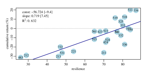
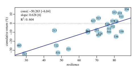
Figure 3 plots the cumulative risk-adjusted returns of value-weighted industry portfolios, ranked by their resilience to pandemics, based on KP’s ‘affected_share’ variable. The figure shows that less resilient industries feature substantially lower cumulative risk-adjusted returns during the COVID-19 crisis: the stocks of the least resilient industries (such as those in NAICS-industry 212: Mining, except oil and gas; 483: Water transportation) generated returns 40% to 50% lower than the most resilient ones (224: Computer and electronic products; 511: Publishing industries, except Internet), depending on the risk adjustment. The cross-sectional relationship between pandemic resilience and cumulative returns is not only highly statistically significant in all three panels of the figure, but also economically significant: for instance, a decrease of 10 percentage points in the resilience metric is associated with a drop of 7.2% in the CAPM-adjusted cumulative return. In the Appendix, Figure A.3 shows qualitatively similar results when resilience is measured on the basis of DN’s ‘teleworkable_manual_wage’ variable.
[Insert Figure 3]
4.3 Returns and Firm Resilience before the Disaster
The evidence in the previous section indicates that when the public became aware of the COVID-19 outbreak, stock returns reacted differently depending on companies’ resilience to the social distancing rules triggered by the pandemic. However, in principle investors may have been aware of pandemic risk even before the COVID-19 shock, so that this risk may have to some extent been priced by the stock market in advance. As explained in Section 2, if investors were fully aware of such risk in advance, they should have required lower expected returns on the stocks of pandemic-resilient companies than on those of non-resilient ones, controlling for their respective exposures to other risks. If instead investors had become gradually aware of such risk, one should observe the opposite pattern, namely, the stocks of pandemic-resilient companies outperforming non-resilient ones. Finally, if investors were completely unaware of such risk, one should not detect any difference in the stock market performance of the two types of companies, prior to the pandemic.
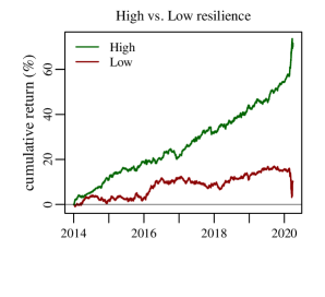
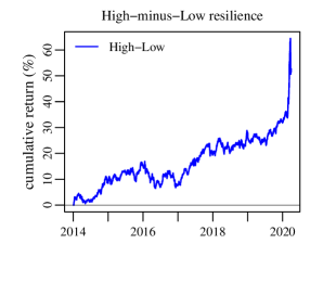
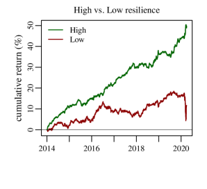
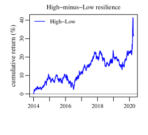
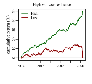
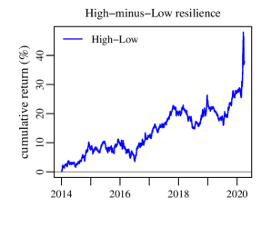
Figure 4 provides evidence on this point, by displaying the time series pattern of risk-adjusted cumulative returns for High- and Low-resilience stocks for six years before the COVID-19 crisis, as well as for a High-minus-Low-resilience portfolio.555The empirical approach is the same as before, i.e. we estimate exposure from daily excess returns over a calendar year and use these exposures to compute risk-adjusted returns in the next year. Irrespective of the risk adjustment considered (CAPM, FF3 or FF5), the figure shows that High-resilience stocks vastly outperformed Low-resilience ones, with most of the differential return stemming from the outperformance of the former rather than the underperformance of the latter. Moreover, about half of the cumulative risk-adjusted return differential between the two portfolios over the whole interval from 2014 to early 2020 materialized before the COVID-19 crisis, the spike occurring during the crisis accounting for the other half.
[Insert Figure 4]
Hence, this evidence appears consistent with the third hypothesis outlined in Section 2, namely, that investors have become gradually aware of disaster risk before the current pandemics, and therefore have sought to acquire the stocks of pandemic-resilient stocks at increasingly high prices, to insulate their portfolios against this previously unknown type of risk.
4.4 Option-Implied Expected Returns after the Disaster
To study how the market prices resilience to disaster risk going forward, we rely on equity options data. Options prices are observable in real time and inherently forward-looking. These features are especially useful in the current crisis, in which – due to its unprecedented nature – relying on historical data appears particularly questionable.
Recent research shows how prices of index options and stock options can be used to compute measures of expected market returns and expected stock returns. In our analysis, we follow the approaches suggested by Martin (2017) and Martin and Wagner (2019). Martin (2017) argues that the risk-neutral variance of the market provides a lower bound on the equity premium. He also argues that, empirically, the lower bound is approximately tight, so that the risk-neutral variance of the market directly measures the equity premium. Martin and Wagner (2019) derive a formula for the expected return on a stock in terms of the risk-neutral variance of the market and the stock’s excess risk-neutral variance relative to that of the average stock.
The three measures of risk-neutral variance – for the market, a particular stock and the average stock – can be computed from option prices using the approach of Breeden and Litzenberger (1978). The market risk-neutral variance, , is determined by the prices of index options:
where is the gross riskfree rate, and denote the spot and forward (to time ) prices of the market, and and denote the time prices of European puts and calls on the market that expire at time with strike . The length of the time interval from to corresponds to the maturity of the options used in the computation.
The risk-neutral variance at the individual stock level, , is defined in terms of individual stock option prices:
where the subscripts indicate the underlying stock .
Finally, using for all firms available at time , we calculate the risk-neutral average stock variance index as .
Using these three risk-neutral variances, one can compute the expected return on a stock using the formula derived by Martin and Wagner (2019):
where denotes the one period gross return on stock . Hence, in the cross-section, differences in expected returns reflect variation in .
In our analysis of expected returns, we use the measures proposed by KP, DN, and HLR to construct risk-neutral variance indices for firms with high resilience to disaster risk, , and for firms with low resilience . For every day in our sample, we compute these indices for each resilience measure as the value-weighted sum of the underlying firms’ , for maturities ranging from 30 to 730 days. We present results for all stocks for which options are available in OptionMetrics, but to face possible concerns about limited trading in options on small stocks we also present results for the subset of S&P 500 firms in the Appendix.
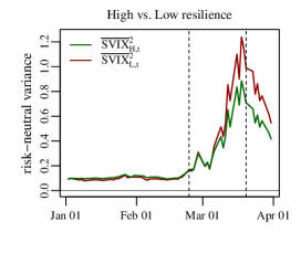
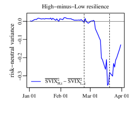
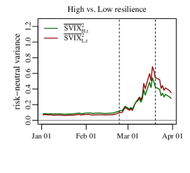
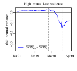
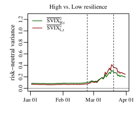
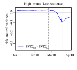
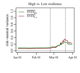
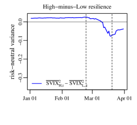
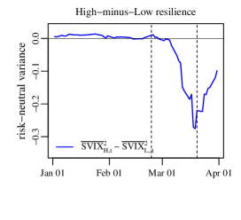
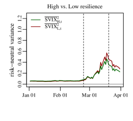
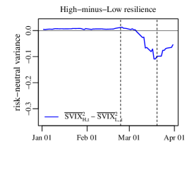
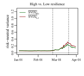
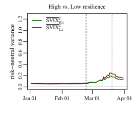
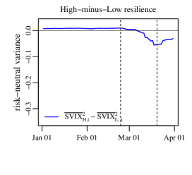
Figure 5 plots the time series of and , measuring resilience on the basis of KP’s ‘affected_share’ measure, as well as their difference for maturities of 30, 91, 365 and 730 days. The results show that, until early March, the options-implied variance of High-resilience stocks slightly exceeded that for Low-resilience stocks. At the time of the Italian lockdown (February 24), the approximate 2% (p.a.) difference implies that High-resilience firms had higher expected returns than Low-resilience ones. During the Covid-19 crisis, the sign of this premium reverses and its magnitude surges to more than 30% (p.a.) at the peak, as implied by one-month options decreasing with longer maturities to approximately 8% (p.a.) for a forecast horizon of two years. Until the end of March these premia gradually declined to half (interestingly, starting shortly before the reversal in stock prices) and imply, as of March 31, that the stocks of Low-resilience firms are expected to carry a premium of about 5.5% (p.a.) over the next year and about 4% (p.a.) over the next two years. The results are qualitatively very similar when only large firms (i.e., constituents of the S&P 500) are retained in the sample, although these firms feature lower -levels, as shown in Figure A.4 of the Appendix.
[Insert Figure 5]
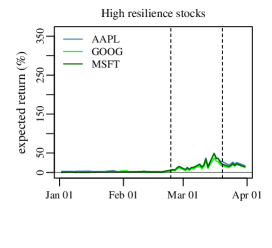
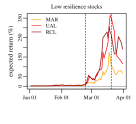
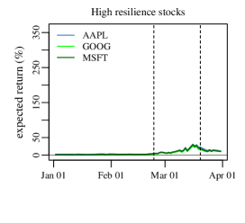
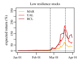
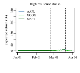
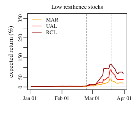
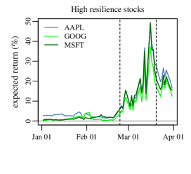
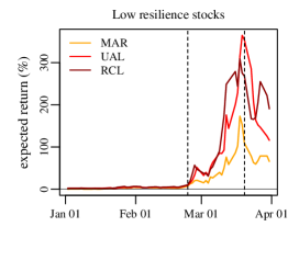
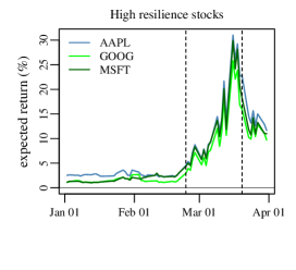
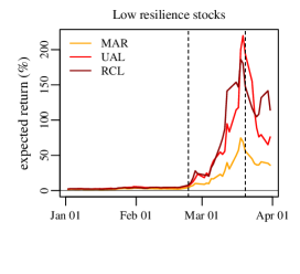
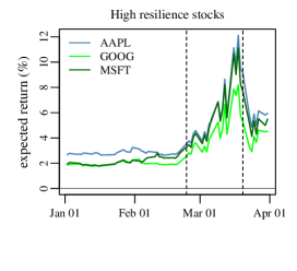
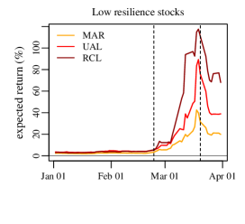
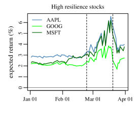
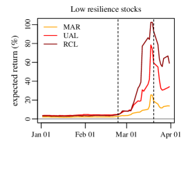
To illustrate these results with reference to some well-known stocks, Figure 6 presents the expected returns of a selected group of S&P firms, respectively featuring high and low resilience to the pandemic, plotting all of them on the same scale, for all stocks and maturities. As examples of very high-resilience firms, the figure plots the option-implied expected returns of Apple, Google, and Microsoft. At the opposite end of the resilience range, as examples of very low-resilience stocks, the figure plots the expected returns of Marriott, United Airlines and Royal Caribbean: travel and tourism have been among the industries hardest hit by the stay-at-home orders and social distancing rules.
[Insert Figure 6]
Two results emerge strikingly from Figure 6. First, at the outbreak of the COVID-19 crisis, all the option-implied expected returns rose, but those of low-resilience stocks (right-side charts) increased by an order of magnitude more than those of low-resilience ones (left-side charts). At the peak of the crisis, the expected return implied by short-term options became an enormous 300% (p.a.) for United Airlines and Royal Caribbean, reflecting unprecedented uncertainty about the immediate future of their businesses. Second, this increase is much more persistent for low-resilience stocks: at the end of our sample, on March 31, their expected returns are still elevated, while for high-resilience stocks they revert back to pre-COVID-19 levels, especially for the two-year horizon. Third, for all stocks expected returns decrease in levels as maturities increase, indicating that there is a term structure to pandemic risk: it is perceived to decrease substantially as the horizon lengthens, though it far from vanishes for low-resilience stocks.
Figure 7 provides a clearer view of the time-series patterns of the expected returns of the six stocks, as it adapts the vertical scale of the plot to their range of variation. The figure allows in particular to appreciate that, even at the end of our sample, almost two months after the outbreak, investors still require much higher expected returns from Marriott, United Airlines and Royal Caribbean than from Apple, Google and Microsoft, and that even at the two-year horizon the expected return is a multiple of what it was at the beginning of the year before the COVID-19 crisis. The most extreme case is Royal Caribbean, whose two-year options imply, as of March 31, an expected return of 60% (p.a.) for a two-year horizon.
[Insert Figure 7]
Taken together, these results indicate that disaster resilience is priced in equity options and that the COVID-19 crisis has greatly affected how financial markets price resilience to disaster risk: While the two-year expected returns have reverted to their pre-crisis levels for the firms least affected by social distancing requirements, the expected returns for the firms most severely affected by the pandemic are much higher than before the crisis. Hence, it appears that, going forward, markets consider disaster risk, and specifically the resilience against a pandemic, to be much more important than they did before COVID-19.
5 Conclusions
The contribution of this paper is threefold. First, it investigates whether the COVID-19 outbreak triggered a different stock return response depending on companies’ resilience to social distancing, which is the most severe constraint that the pandemic has imposed on firms’ operations. On this score, we find that more resilient companies greatly outperformed less resilient ones, even after controlling for all conventional measures of risk premia.
Second, the paper explores whether similar cross-sectional return differentials already emerged before the COVID-19 outbreak. Indeed this is the case: in the 2014-19 interval, the cumulative return differential between more and less pandemic-resilient firms is of about the same magnitude as during the outbreak, i.e. between late February and early April 2020. We interpret this as evidence of learning by investors, i.e., of their growing awareness of the potential threat posed by pandemics well in advance of its materialization.
Finally, we exploit option price data to infer whether, after the COVID-19 outbreak, investors price pandemic risk over different horizons, and find that they do: even on a 2-year horizon, stocks of more pandemic-resilient firms are expected to yield significantly lower returns than less resilient ones, reflecting lower exposure to disaster risk. Such differences are massive in the case of some stocks: for example, as late as early April 2020, the expected return on low-resilience stocks such as Royal Caribbean and United Airlines is around 60% and 40% respectively, while those of high-resilience stocks such as Apple and Microsoft are between 3% and 4%.
Hence, going forward, markets appear to price exposure to a new risk factor, namely, pandemic risk. In future development of this work, we plan to investigate whether such risk is part of a wider sustainability risk factor, or at least whether the two types of risk are correlated. We also plan to investigate whether resilience to social distancing has not only direct effects on stock prices, but also indirect effects via demand and supply linkages, i.e. whether for instance the stocks of firms that depend heavily on low-resilience firms are themselves more exposed to pandemic risk, other things equal.
References
- Albuquerque et al. (2020) Albuquerque, R. A., Y. Koskinen, S. Yang, and C. Zhang. 2020. Resiliency of environmental and social stocks: an analysis of the exogenous COVID-19 market crash. Available at SSRN 3583611 .
- Alfaro et al. (2020) Alfaro, L., A. Chari, A. Greenland, and P. Schott. 2020. Aggregate and firm-level stock returns during pandemics. Available at SSRN 3562034 .
- Andrews (1991) Andrews, D. W. K. 1991. Heteroskedasticity and Autocorrelation Consistent Covariance Matrix Estimation. Econometrica 59:817–858.
- Barro (2006) Barro, R. J. 2006. Rare Disasters and Asset Markets in the Twentieth Century. The Quarter Journal of Economics 121:823–866.
- Barro (2009) Barro, R. J. 2009. Rare Disasters, Asset Prices, and Welfare Costs. American Economic Review 99:243–64.
- Breeden and Litzenberger (1978) Breeden, D. T., and R. H. Litzenberger. 1978. Prices of state-contingent claims implicit in option prices. Journal of Business pp. 621–651.
- Bretscher et al. (2020) Bretscher, L., A. Hsu, and A. Tamoni. 2020. The Supply Channel of Uncertainty Shocks and the Cross-Section of Returns: Evidence From the COVID-19 Crisis. Available at SSRN 3588418 .
- Carhart (1997) Carhart, M. M. 1997. On persistence in mutual fund performance. The Journal of finance 52:57–82.
- Coibion et al. (2020a) Coibion, O., Y. Gorodnichenko, and M. Weber. 2020a. The Cost of the COVID-19 Crisis: Lockdowns, Macroeconomic Expectations, and Consumer Spending. Chicago Booth Research Paper .
- Coibion et al. (2020b) Coibion, O., Y. Gorodnichenko, and M. Weber. 2020b. Labor Markets During the COVID-19 Crisis: A Preliminary View. Tech. rep., National Bureau of Economic Research.
- Croce et al. (2020) Croce, M. M. M., P. Farroni, and I. Wolfskeil. 2020. When the markets get covid: Contagion, viruses, and information diffusion. Available at SSRN 3560347 .
- Ding et al. (2020) Ding, W., R. Levine, C. Lin, and W. Xie. 2020. Corporate Immunity to the COVID-19 Pandemic. NBER Working Paper 27055 .
- Dingel and Neiman (2020) Dingel, J., and B. Neiman. 2020. How many jobs can be done at home? NBER Working Paper 26948 .
- Fama and French (1993) Fama, E. F., and K. R. French. 1993. Common Risk Factors in the Returns on Stocks and Bonds. Journal of Financial Economics 33:3–56.
- Fama and French (2015) Fama, E. F., and K. R. French. 2015. A Five-Factor Asset Pricing Model. Journal of Financial Economics 116:1–22.
- Gabaix (2012) Gabaix, X. 2012. Variable Rare Disasters: An Exactly Solved Framework for Ten Puzzles in Macro-Finance. The Quarterly Journal of Economics 127:645–700.
- Gerding et al. (2020) Gerding, F., T. Martin, and F. Nagler. 2020. The value of fiscal capacity in the face of a rare disaster. Available at SSRN 3572839 .
- Gillman et al. (2014) Gillman, M., M. Kejak, and M. Pakoš. 2014. Learning about Rare Disasters: Implications For Consumption and Asset Prices. Review of Finance 19:1053–1104.
- Gormsen and Koijen (2020) Gormsen, N. J., and R. S. Koijen. 2020. Coronavirus: Impact on stock prices and growth expectations. University of Chicago, Becker Friedman Institute for Economics Working Paper .
- Hanspal et al. (2020) Hanspal, T., A. Weber, and J. Wohlfart. 2020. Income and Wealth Shocks and Expectations during the COVID-19 Pandemic. CEBI Working Paper Series .
- Hassan et al. (2020) Hassan, T. A., S. Hollander, L. van Lent, and A. Tahoun. 2020. Firm-level Exposure to Epidemic Diseases: Covid-19, SARS, and H1N1. NBER Working Paper 26971 .
- Hensvik et al. (2020) Hensvik, L., T. Le Barbanchon, and R. Rathelot. 2020. Which jobs are done from home? Evidence from the American Time Use Survey. CEPR Discussion Paper14611 .
- Koren and Pető (2020) Koren, M., and R. Pető. 2020. Business disruptions from social distancing. Covid Economics 2 pp. 13–31.
- Lu and Siemer (2016) Lu, Y. K., and M. Siemer. 2016. Learning, Rare Disasters, and Asset Prices. Tech. Rep. 1977867, SSRN.
- Lucas (1978) Lucas, R. E. 1978. Asset prices in an exchange economy. Econometrica: Journal of the Econometric Society pp. 1429–1445.
- Martin (2017) Martin, I. 2017. What is the Expected Return on the Market? The Quarterly Journal of Economics 132:367–433.
- Martin and Wagner (2019) Martin, I. W., and C. Wagner. 2019. What is the Expected Return on a Stock? The Journal of Finance 74:1887–1929.
- Newey and West (1987) Newey, W. K., and K. D. West. 1987. A Simple, Positive Semi-Definite, Heteroskedasticity and Autocorrelation Consistent Covariance Matrix. Econometrica 55:703–708.
- Pastor et al. (2020) Pastor, L., R. F. Stambaugh, and L. A. Taylor. 2020. Sustainable Investing in Equilibrium. Working Paper .
- Ramelli and Wagner (2020) Ramelli, S., and A. F. Wagner. 2020. Feverish stock price reactions to Covid-19 .
- Rietz (1988) Rietz, T. A. 1988. The equity risk premium a solution. Journal of monetary Economics 22:117–131.
- Ru et al. (2020) Ru, H., E. Yang, and K. Zou. 2020. What Do We Learn from SARS-CoV-1 to SARS-CoV-2: Evidence from Global Stock Markets. Available at SSRN 3569330 .
- Veronesi (2004) Veronesi, P. 2004. The peso problem hypothesis and stock market returns. Journal of Economic Dynamics and Control 28:707–725.
- Wachter (2013) Wachter, J. A. 2013. Can time-varying risk of rare disasters explain aggregate stock market volatility? The Journal of Finance 68:987–1035.
- Wachter and Zhu (2019) Wachter, J. A., and Y. Zhu. 2019. Learning with Rare Disasters. Tech. Rep. 3407397, SSRN.
- White (1980) White, H. 1980. A Heteroskedasticity-Consistent Covariance Matrix Estimator and a Direct Test for Heteroscedasticity. Econometrica 48:817–838.
- Xu and Li (2020) Xu, S., and Y. Li. 2020. Beware of the Second Wave of COVID-19. The Lancet 395:1321–1322.
Panel A illustrates the attention to Covid19 in the United States, as measured by the Google trends index for the term “Coronavirus” in the US, and the cumulative returns of the US stock market, as measured by the Fama-French market factor, during the first quarter of 2020. Panel B plots the cumulative returns of portfolios sorted by firms’ resilience to disaster risk. On any given day, we assign a firm to the ‘High’ portfolio if its ‘affected_share’ (as defined by Koren and Pető, 2020) is below the median value and to the ‘Low’ portfolio if it is above. We plot the cumulative value-weighted portfolio returns for the ‘High’ portfolio (in green) and the Low portfolio (in red) as well as the High-Low differential return (in blue). The dashed vertical lines mark February 24, the day after Italy introduced its lockdown, and March 20, the last trading day before the Fed announced its intervention.
Panel A. Google trends index and aggregate US stock market
Panel B. Excess returns of firms with high and low resilience to social distancing
This figure plots the cumulative risk-adjusted returns of portfolios sorted by firms’ resilience to disaster risk during the first quarter of 2020. On any given day, we assign a firm to the ‘High’ portfolio if its ‘affected_share’ (as defined by Koren and Pető, 2020) is below the median value and to the ‘Low’ portfolio if it is above. In Panel A, we present CAPM-adjusted returns, i.e. controlling for exposure to market risk. Panels B and C present results controlling for the Fama-French three factor model exposures (i.e. market, size, value) and five factor model exposures (i.e. market, size, value, investments, profitability), respectively. We plot the cumulative value-weighted portfolio returns for the ‘High’ portfolio (in green) and the Low portfolio (in red) as well as the High-Low differential return (in blue). The dashed vertical lines mark February 24, the day after Italy introduced its lockdown, and March 20, the last trading day before the Fed announced its intervention.
Panel A. CAPM-adjusted returns
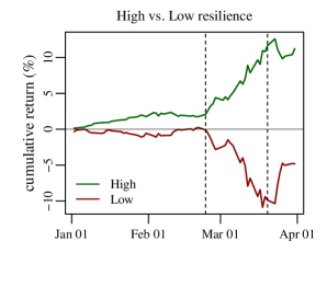
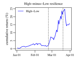
Panel B. FF3-adjusted returns
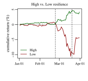
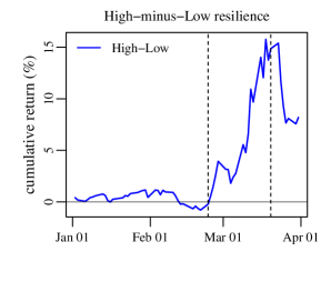
Panel C. FF5-adjusted returns
This figure plots the cumulative risk-adjusted returns of value-weighted industry portfolios against the industries’ resilience to disaster risk. The sample period is from February 24 to March 20, 2020, i.e. from the day after Italy introduced its lockdown to the last trading day before the Fed announced its intervention. We define resilience as 100 (%) minus the ‘affected_share’ defined by Koren and Pető (2020) and present results for the 25 industries with the highest number of firms (in total 2,974). In Panel A, we present CAPM-adjusted returns, i.e. controlling for exposure to market risk. Panels B and C present results controlling for the Fama-French three factor model exposures (i.e. market, size, value) and five factor model exposures (i.e. market, size, value, investments, profitability), respectively. The plot labels indicate the industries’ 3-digit NAICS codes. The plot legends report results for cross-sectional regressions with -statistics based on White (1980) standard errors in square brackets.
Panel A. CAPM-ajdusted returns
Panel B. FF3-ajdusted returns
Panel C. FF5-ajdusted returns

This figure plots the cumulative risk-adjusted returns of portfolios sorted by firms’ resilience to disaster risk during from January 2014 through March 2020. On any given day, we assign a firm to the ‘High’ portfolio if its ‘affected_share’ (as defined by Koren and Pető, 2020) is below the median value and to the ‘Low’ portfolio if it is above. In Panel A, we present CAPM-adjusted returns, i.e. controlling for exposure to market risk. Panels B and C present results controlling for the Fama-French three factor model exposures (i.e. market, size, value) and five factor model exposures (i.e. market, size, value, investments, profitability), respectively. We plot the cumulative value-weighted portfolio returns for the ‘High’ portfolio (in green) and the Low portfolio (in red) as well as the High-Low differential return (in blue).
Panel A. CAPM-adjusted returns
Panel B. FF3-adjusted returns
Panel C. FF5-adjusted returns
This figure plots stock options-implied risk-neutral variance indices for firms with high and low resilience to social distancing during the first quarter of 2020. On any given day, we assign a firm to the high resilience index, , if its ‘affected_share’ (as defined by Koren and Pető, 2020) is below the median value and to the low resilience index, , if it is above. The indices are computed as the value-weighted sums of individual firms’ risk-neutral variances, . The difference measures the expected return of low resilience in excess of high resilience stocks. Panels A to D present results using options maturities of 30, 91, 365 and 730 days, respectively. The dashed vertical lines mark February 24 and March 20.
Panel A. 30-day horizon
Panel B. 91-day horizon
Panel C. 365-day horizon
Panel D. 730-day horizon
This figure plots stock options-implied expected returns for selected S&P 500 firms during the first quarter of 2020. The high resilience stocks we consider are Apple (AAPL), Google (GOOG), and Microsoft (MSFT), the low resilience stocks are Marriott (MAR), United Airlines (UAL) and Royal Caribbean (RCL). We compute the expected return on a stock in from the risk-neutral variance of the market and the stock’s excess risk-neutral variance relative to that of the average stock following the approach of Martin and Wagner (2019). Panels A to D present results for forecast horizons of 30, 91, 365 and 730 days, respectively. The dashed vertical lines mark February 24 and March 20.
Panel A. 30-day horizon
Panel B. 91-day horizon
Panel C. 365-day horizon
Panel D. 730-day horizon

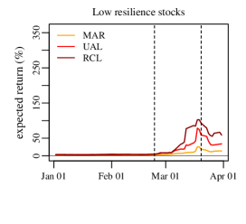
This figure plots stock options-implied expected returns for selected S&P 500 firms during the first quarter of 2020. The high resilience stocks we consider are Apple (AAPL), Google (GOOG), and Microsoft (MSFT), the low resilience stocks are Marriott (MAR), United Airlines (UAL) and Royal Caribbean (RCL). We compute the expected return on a stock in from the risk-neutral variance of the market and the stock’s excess risk-neutral variance relative to that of the average stock following the approach of Martin and Wagner (2019). Panels A to D present results for forecast horizons of 30, 91, 365 and 730 days, respectively. The dashed vertical lines mark February 24 and March 20.
Panel A. 30-day horizon
Panel B. 91-day horizon
Panel C. 365-day horizon
Panel D. 730-day horizon
This table reports averages of daily returns for value-weighted portfolios of low and high resilience stocks from February 24 to March 20, 2020, i.e. from the day after Italy introduced its lockdown to the last trading day before the Fed announced its intervention. On any given day, we assign a firm to the ‘High’ (‘Low’) portfolio, in Panel A, if its ‘affected_share’ (as defined by Koren and Pető, 2020) is below (above) the median value; in Panel B, if its ‘teleworkable_manual_wage’ (as defined by Dingel and Neiman, 2020) is above (below) the median value; in Panel C, if its ‘dur_workplace’ (as defined by Hensvik et al., 2020) is below (above) the median value. and to the ‘Low’ portfolio if it is above. In addition to rae excess returns (ret), we report CAPM-adjusted returns, i.e. controlling for exposure to market risk, returns adjusted for the Fama-French three factor model exposures (ff3, i.e. market, size, value) and five factor model exposures (ff5, i.e. market, size, value, investments, profitability), and the Fama-French models augmented by the momentum factor (ff4 and ff6). Values in square brackets are -statistics based on standard errors following Newey and West (1987), where we choose the optimal truncation lag as suggested by Andrews (1991). ∗, ∗∗ and ∗∗∗ denote statistical significance at the 10%, 5%, and 1% level, respectively.
Panel A. Resilience based on ‘affected_share’ as in Koren and Pető (2020)
| ret | capm | ff3 | ff4 | ff5 | ff6 | |
| High resilience | ||||||
| [-3.02] | [6.65] | [2.69] | [2.06] | [3.04] | [2.29] | |
| Low resilience | ||||||
| [-3.84] | [-3.00] | [-2.89] | [-2.65] | [-2.90] | [-2.70] | |
| High-minus-Low | ||||||
| [3.22] | [4.26] | [2.94] | [2.65] | [3.12] | [2.85] |
Panel B. Resilience based on ‘teleworkable_manual_wage’ as in Dingel and Neiman (2020)
| ret | capm | ff3 | ff4 | ff5 | ff6 | |
| High resilience | ||||||
| [-3.65] | [3.36] | [0.59] | [0.32] | [1.24] | [1.06] | |
| Low resilience | ||||||
| [-3.43] | [-2.03] | [-2.11] | [-1.86] | [-2.36] | [-2.27] | |
| High-minus-Low | ||||||
| [1.16] | [2.69] | [1.66] | [1.28] | [2.22] | [2.09] |
Panel C. Resilience based on ‘dur_workplace’ as in Hensvik et al. (2020)
| ret | capm | ff3 | ff4 | ff5 | ff6 | |
| High resilience | ||||||
| [-3.34] | [4.64] | [0.77] | [0.63] | [1.11] | [1.12] | |
| Low resilience | ||||||
| [-3.73] | [-2.53] | [-2.10] | [-2.09] | [-2.01] | [-2.11] | |
| High-minus-Low | ||||||
| [3.40] | [3.90] | [1.67] | [1.61] | [1.92] | [1.99] |
This table presents summary statistics for the returns of value-weighted industry portfolios from February 24 to March 20, 2020, i.e. from the day after Italy introduced its lockdown to the last trading day before the Fed announced its intervention. We define resilience as 100 (%) minus the ‘affected_share’ defined by Koren and Pető (2020) and present results for the 25 industries with the highest number of firms (in total 2,974). We report the industries’ 3-digit NAICS code, their description, the number of firms in the respective industries and their cumulative return. Specifically, we present CAPM-adjusted returns, i.e. controlling for exposure to market risk as well as results controlling for the Fama-French three factor model exposures (ff3, i.e. market, size, value) and five factor model exposures (ff5, i.e. market, size, value, investments, profitability).
| NAICS | description | firms | resilience | capm | ff3 | ff5 |
|---|---|---|---|---|---|---|
| 211 | Oil and gas extraction | 88 | 70 | |||
| 212 | Mining, except oil and gas | 87 | 29 | |||
| 213 | Support activities for mining | 37 | 46 | |||
| 221 | Utilities | 94 | 54 | |||
| 311 | Food manufacturing | 53 | 77 | |||
| 325 | Chemicals | 639 | 79 | |||
| 332 | Fabricated metal products | 54 | 79 | |||
| 333 | Machinery | 118 | 80 | |||
| 334 | Computer and electronic products | 327 | 87 | |||
| 335 | Electrical equipment and appliances | 44 | 83 | |||
| 336 | Transportation equipment | 97 | 81 | |||
| 339 | Miscellaneous durable goods manufacturing | 89 | 84 | |||
| 423 | Wholesale trade: Durable goods | 58 | 68 | |||
| 424 | Wholesale trade: Nondurable goods | 49 | 71 | |||
| 483 | Water transportation | 52 | 26 | |||
| 511 | Publishing industries, except Internet | 92 | 84 | |||
| 515 | Broadcasting, except Internet | 71 | 65 | |||
| 518 | Data processing, hosting and related services | 71 | 81 | |||
| 519 | Other information services | 161 | 76 | |||
| 523 | Securities, commodity contracts, investments, and funds and trusts | 136 | 71 | |||
| 524 | Insurance carriers and related activities | 127 | 72 | |||
| 531 | Real estate | 222 | 48 | |||
| 541 | Professional and technical services | 104 | 77 | |||
| 561 | Administrative and support services | 57 | 65 | |||
| 722 | Food services and drinking places | 47 | 47 |
Appendix for
“Disaster Resilience and Stock Returns”
Marco Pagano Christian Wagner Josef Zechner
This Appendix provides additional results referred to in the paper.
This figure plots the cumulative risk-adjusted returns of portfolios sorted by firms’ resilience to disaster risk during the first quarter of 2020. On any given day, we assign a firm to the ‘High’ portfolio if its ‘teleworkable_manual_wage’ (as defined by Dingel and Neiman, 2020) is above the median value and to the ‘Low’ portfolio if it is below. In Panel A, we present CAPM-adjusted returns, i.e. controlling for exposure to market risk. Panels B and C present results controlling for the Fama-French three factor model exposures (i.e. market, size, value) and five factor model exposures (i.e. market, size, value, investments, profitability), respectively. We plot the cumulative value-weighted portfolio returns for the ‘High’ portfolio (in green) and the Low portfolio (in red) as well as the High-Low differential return (in blue). The dashed vertical lines mark February 24, the day after Italy introduced its lockdown, and March 20, the last trading day before the Fed announced its intervention.
Panel A. CAPM-adjusted returns
Panel B. FF3-adjusted returns
Panel C. FF5-adjusted returns
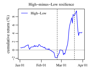
This figure plots the cumulative risk-adjusted returns of portfolios sorted by firms’ resilience to disaster risk during the first quarter of 2020. On any given day, we assign a firm to the ‘High’ portfolio if its ‘dur_workplace’ (as defined by Hensvik et al., 2020) is below the median value and to the ‘Low’ portfolio if it is above. In Panel A, we present CAPM-adjusted returns, i.e. controlling for exposure to market risk. Panels B and C present results controlling for the Fama-French three factor model exposures (i.e. market, size, value) and five factor model exposures (i.e. market, size, value, investments, profitability), respectively. We plot the cumulative value-weighted portfolio returns for the ‘High’ portfolio (in green) and the Low portfolio (in red) as well as the High-Low differential return (in blue). The dashed vertical lines mark February 24, the day after Italy introduced its lockdown, and March 20, the last trading day before the Fed announced its intervention.
Panel A. CAPM-adjusted returns
Panel B. FF3-adjusted returns
Panel C. FF5-adjusted returns
This figure plots the cumulative risk-adjusted returns of value-weighted industry portfolios against the industries’ resilience to disaster risk. The sample period is from February 24 to March 20, 2020, i.e. from the day after Italy introduced its lockdown to the last trading day before the Fed announced its intervention. We define resilience as 100 (%) minus the ‘teleworkable_manual_wage’ defined by Dingel and Neiman (2020) and present results for the 25 industries with the highest number of firms (in total 2,974). In Panel A, we present CAPM-adjusted returns, i.e. controlling for exposure to market risk. Panels B and C present results controlling for the Fama-French three factor model exposures (i.e. market, size, value) and five factor model exposures (i.e. market, size, value, investments, profitability), respectively. The plot labels indicate the industries’ 3-digit NAICS codes. The plot legends report results for cross-sectional regressions with -statistics based on White (1980) standard errors in square brackets.
Panel A. CAPM-ajdusted returns
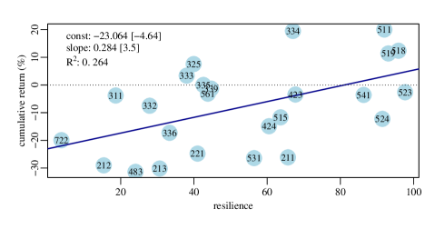
Panel B. FF3-ajdusted returns
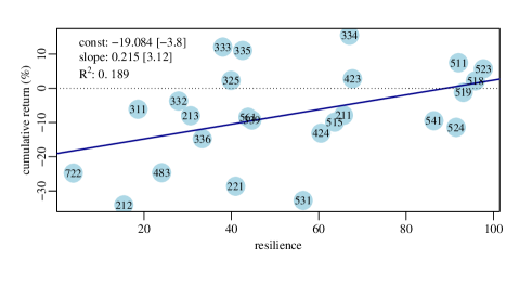
Panel C. FF5-ajdusted returns

This figure plots stock options-implied risk-neutral variance indices for S&P 500 firms with high and low resilience to social distancing during the first quarter of 2020. On any given day, we assign a firm to the high resilience index, , if its ‘affected_share’ (as defined by Koren and Pető, 2020) is below the median value and to the low resilience index, , if it is above. The indices are computed as the value-weighted sums of individual firms’ risk-neutral variances, . The difference measures the expected return of low resilience in excess of high resilience stocks. Panels A to D present results using options maturities of 30, 91, 365 and 730 days, respectively. The dashed vertical lines mark February 24 and March 20.
Panel A. 30-day horizon
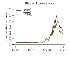
Panel B. 91-day horizon
Panel C. 365-day horizon

Panel D. 730-day horizon
This Table provides an overview of the empirical measures on which we base our analysis of stocks’ disaster resilience. Panel A lists the teleworkability measures provided by Dingel and Neiman (2020) for 24 industries at the NAICS 2-digit level and for 88 industries at the NAICS 3-digit level. Panel B lists the work at home and work at the workplace measures provided by Hensvik et al. (2020) for 310 industries at the NAICS 4-digit level. Panel C lists the communication-intensity and physical proximity measures suggested by Koren and Pető (2020) for 84 industries at the NAICS 3-digit level.
Panel A. Dingel and Neiman (2020):
| ‘teleworkable_emp’ | fraction of jobs that can be done from home estimated from O*Net data |
| ‘teleworkable_wage’ | fraction of wages to jobs that can be done from home estimated from O*Net data |
| ‘teleworkable_manual_emp’ | fraction of jobs that can be done from home based on manual classification by the authors |
| ‘teleworkable_manual_wage’ | fraction of wages to jobs that can be done from home based on manual classification by the authors |
Panel B. Hensvik et al. (2020)
| ‘home’ | fraction of respondents that work at home |
| ‘workplace’ | fraction of respondents that work at workplace |
| ‘dur_home’ | hours worked at home per day |
| ‘dur_workplace’ | hours worked at workplace per day |
| ‘share_home’ | hours worked at home divided by hours worked at home and at workplace |
Panel C. Koren and Pető (2020)
| ‘teamwork_share’ | percentage of workers in teamwork-intensive occupations, i.e. internal communication |
| ‘customer_share’ | percentage of workers in customer-facing occupations, i.e. external communication |
| ‘communication_share’ | percentage of workers in teamwork-intensive and/or customer-facing occupations |
| ‘presence_share’ | percentage of workers whose jobs require physical presence in close proximity to others |
| ‘affected_share’ | percentage of workers in occupations that are communication-intensive and/or require physical presence in close proximity to others |
This table presents results analogous to Panel A in Table 2 but using the other measures constructed by Koren and Pető (2020) instead of their ‘affected_share’ variable.
Panel A. Portfolios sorted by ‘teamwork_share’
| ret | capm | ff3 | ff4 | ff5 | ff6 | |
| High resilience | ||||||
| [-3.79] | [2.72] | [0.75] | [0.44] | [1.48] | [1.58] | |
| Low resilience | ||||||
| [-3.38] | [-2.00] | [-2.42] | [-2.35] | [-2.37] | [-2.33] | |
| High-minus-Low | ||||||
| [1.01] | [2.58] | [2.21] | [2.06] | [2.35] | [2.27] |
Panel B. Portfolios sorted by ‘customer_share’
| ret | capm | ff3 | ff4 | ff5 | ff6 | |
| High resilience | ||||||
| [-3.33] | [4.51] | [4.10] | [0.26] | [3.24] | [-0.14] | |
| Low resilience | ||||||
| [-3.36] | [-0.74] | [-3.49] | [-2.87] | [-4.14] | [-3.94] | |
| High-minus-Low | ||||||
| [0.96] | [15.17] | [6.51] | [2.69] | [9.94] | [5.07] |
Panel C. Portfolios sorted by ‘communication_share’
| ret | capm | ff3 | ff4 | ff5 | ff6 | |
| High resilience | ||||||
| [-3.39] | [5.46] | [15.28] | [0.89] | [3.61] | [0.19] | |
| Low resilience | ||||||
| [-3.63] | [-2.06] | [-3.74] | [-3.67] | [-3.85] | [-3.96] | |
| High-minus-Low | ||||||
| [2.02] | [5.62] | [5.61] | [6.72] | [6.14] | [12.44] |
Panel D. Portfolios sorted by ‘presence_share’
| ret | capm | ff3 | ff4 | ff5 | ff6 | |
| High resilience | ||||||
| [-3.63] | [3.09] | [1.07] | [0.85] | [2.49] | [2.80] | |
| Low resilience | ||||||
| [-3.78] | [-3.31] | [-3.05] | [-2.98] | [-3.16] | [-3.14] | |
| High-minus-Low | ||||||
| [2.90] | [3.57] | [2.68] | [2.50] | [3.27] | [3.23] |
This table presents results analogous to Panel B in Table 2 but using the other measures constructed by Dingel and Neiman (2020) instead of their ‘teleworkable_manual_wage’ variable.
Panel A. Portfolios sorted by “teleworkable_wage”
| ret | capm | ff3 | ff4 | ff5 | ff6 | |
| High resilience | ||||||
| [-3.67] | [2.80] | [0.40] | [-0.12] | [1.46] | [0.65] | |
| Low resilience | ||||||
| [-3.24] | [-1.59] | [-1.77] | [-1.39] | [-2.08] | [-1.89] | |
| High-minus-Low | ||||||
| [0.06] | [2.20] | [1.36] | [0.81] | [1.99] | [1.67] |
Panel B. Portfolios sorted by “teleworkable_manual_emp”
| ret | capm | ff3 | ff4 | ff5 | ff6 | |
| High resilience | ||||||
| [-3.34] | [3.74] | [-0.23] | [-0.32] | [-0.37] | [-0.14] | |
| Low resilience | ||||||
| [-3.60] | [-1.80] | [-1.74] | [-1.70] | [-1.60] | [-1.78] | |
| High-minus-Low | ||||||
| [1.56] | [2.93] | [1.02] | [0.96] | [1.21] | [1.41] |
Panel C. Portfolios sorted by “teleworkable_emp”
| ret | capm | ff3 | ff4 | ff5 | ff6 | |
| High resilience | ||||||
| [-3.25] | [3.14] | [-0.51] | [-0.81] | [-0.94] | [-1.00] | |
| Low resilience | ||||||
| [-3.53] | [-1.44] | [-1.66] | [-1.41] | [-1.65] | [-1.67] | |
| High-minus-Low | ||||||
| [0.54] | [2.56] | [0.85] | [0.50] | [1.24] | [1.21] |
This table presents results analogous to Panel C in Table 2 but using the other measures constructed by Hensvik et al. (2020) instead of their ‘dur_workplace’ variable.
Panel A. Portfolios sorted by ‘workplace’
| ret | capm | ff3 | ff4 | ff5 | ff6 | |
| High resilience | ||||||
| [-3.45] | [5.16] | [0.92] | [0.47] | [1.40] | [0.86] | |
| Low resilience | ||||||
| [-3.68] | [-2.40] | [-2.22] | [-1.91] | [-2.22] | [-1.99] | |
| High-minus-Low | ||||||
| [3.17] | [3.77] | [1.87] | [1.28] | [2.11] | [1.75] |
Panel B. Portfolios sorted by ‘dur_home’
| ret | capm | ff3 | ff4 | ff5 | ff6 | |
| High resilience | ||||||
| [-3.46] | [2.53] | [-0.93] | [-0.43] | [-1.54] | [-0.40] | |
| Low resilience | ||||||
| [-3.66] | [-1.58] | [-1.32] | [-1.76] | [-1.12] | [-1.56] | |
| High-minus-Low | ||||||
| [1.88] | [2.71] | [0.33] | [0.89] | [0.40] | [1.16] |
Panel C. Portfolios sorted by ‘home’
| ret | capm | ff3 | ff4 | ff5 | ff6 | |
| High resilience | ||||||
| [-3.49] | [5.89] | [-0.11] | [0.13] | [-0.20] | [0.37] | |
| Low resilience | ||||||
| [-3.77] | [-2.12] | [-1.80] | [-1.98] | [-1.64] | [-1.84] | |
| High-minus-Low | ||||||
| [2.01] | [3.31] | [1.23] | [1.52] | [1.22] | [1.56] |
Panel D. Portfolios sorted by ‘share_home’
| ret | capm | ff3 | ff4 | ff5 | ff6 | |
| High resilience | ||||||
| [-3.73] | [3.69] | [-0.08] | [-0.28] | [-0.14] | [-0.08] | |
| Low resilience | ||||||
| [-3.64] | [-1.88] | [-1.79] | [-1.67] | [-1.66] | [-1.63] | |
| High-minus-Low | ||||||
| [1.63] | [2.85] | [1.09] | [0.90] | [1.23] | [1.19] |