Exceptional Point of Degeneracy in Linear-Beam Tubes for High Power Backward-Wave Oscillators

Abstract

An exceptional point of degeneracy (EPD) is induced in a system made of an electron beam interacting with an electromagnetic (EM) guided mode. This enables a degenerate synchronous regime in backward wave oscillators (BWOs) where the electron beams provides distributed gain to the EM mode with distributed power extraction. Current particle-in-cell simulation results demonstrate that BWOs operating at an EPD have a starting-oscillation current that scales quadratically to a non-vanishing value for long interaction lengths and therefore have higher power conversion efficiency at arbitrarily higher level of power generation compared to standard BWOs.

I Introduction

The characterizing feature of an exceptional point is the singularity resulting from the degenracy of at least two eigenstates. We stress the importance to refer to it as “degeneracy” as implied in [1]. Here an exceptional point of degeneracy (EPD) is demonstrated in a system made of an electron beam interacting with an electromagnetic (EM) guided mode. Despite most of the published work on EPDs are related to parity time (PT) symmetry [2, 3], the occurrence of EPDs does not necessarily require a system to exactly satisfy the PT symmetry condition, however, it generally requires a system to simultaneously have gain and loss [4]. The system we consider in this paper involves two complete different media that support waves: an electron beam (e-beam) for charge waves and a waveguide for EM waves. Exchange of energy occurs when an EM waves in a slow wave structure (SWS) interacts with the e-beam. In this paper the degeneracy condition is enabled by the distributed power extraction (DPE) from the SWS waveguide as shown in Fig. 1. The energy that is extracted from the e-beam and delivered to the guided EM mode is considered as a distributed gain from the SWS prescriptive, whereas the DPE represents extraction “losses” and not mere dissipation [5, 6].

Backward-wave oscillators (BWOs) are high power sources where the power is transferred from a very energetic e-beam to a synchronized EM mode [7]. The extracted power in a conventional BWO is usually taken at one end of the SWS [8, 9] as shown in Fig. 1(a). One challenging issue in BWOs is the limitation in power generation level. Indeed conventional BWOs exhibit small starting beam current (to induce sustained oscillations) and limited power efficiency without reaching very high output power levels [10]. Several techniques were proposed in literature to enhance the power conversion efficiency of BWOs by optimizing the SWS and its termination. For example, non-uniform SWSs were proposed to enhance efficiency of BWOs in [11], in [12] a resonant reflector was used to enhance efficiency to about 30%, and a two-sectional SWS was also proposed to enhance the power efficiency in [13]. Here we propose a regime of operation of BWO based on an EPD that to occurs need a DPE as in Fig. 1(b). In this paper we show the physical mechanism of an EPD arising from the interaction of an e-beam and and EM wave in a SWS and we show how this finding can be used as a regime of operation in what we call an EPD-BWO to produce very high power with high efficiency.

II Theoretical model based on an extension of the Pierce model

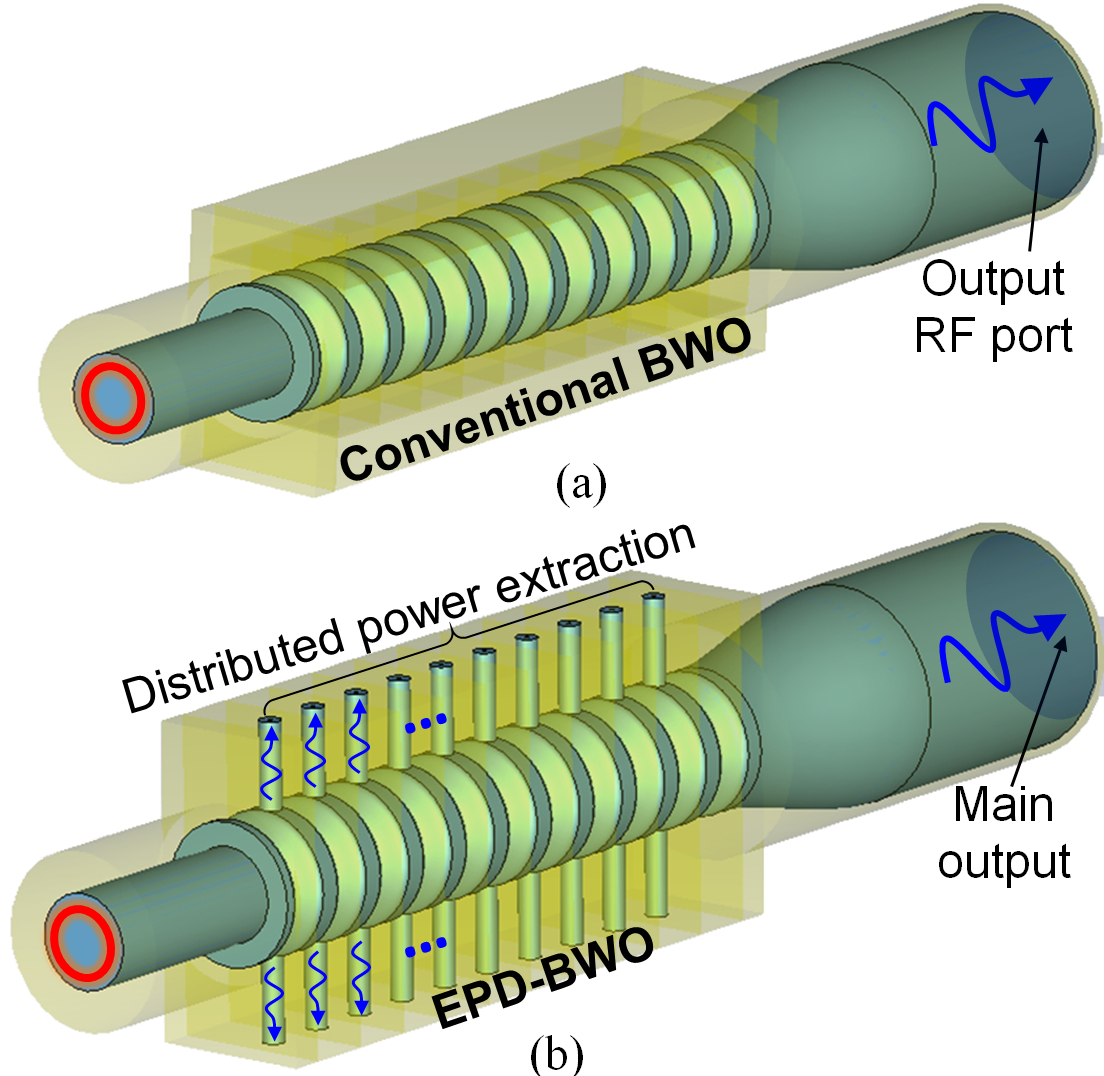
Figure 1: (a) Conventional BWO where the power is extracted from the waveguide end; (b) EPD-BWO where the power is extracted in a distributed fashion to satisfy the EPD condition. The power is extracted using distributed wire loops (as an example) that are connected to coaxial waveguides.

The interaction between the e-beam charge wave and the EM wave in the SWS occurs when they are synchronized, i.e., when the EM wave phase velocity $v_{ph}=\omega/\beta_{p}$ is matched to the average velocity of the electrons $u_{0}$, where $\beta_{p}$ is the phase propagation constants of the “cold” EM wave, i.e., when it is not interacting with the e-beam. The synchronization condition provides an estimate of the oscillation frequency of BWO ( $\omega\approx u_{0}\beta_{p}$ ) and is considered as an initial criterion, because the phase velocity of the “hot” modes, i.e., in the interactive system, are different from $v_{ph}$ and $u_{0}$ due to the interaction [14, 15].

The interaction between the e-beam and the EM wave in vacuum tube devices was theoretically studied by Pierce in [14]. Assuming a wave eigenfunctions of the interactive system of infinite length in the form of $\phi(z,t)\propto e^{i\omega t-ikz}$, Pierce showed that the solutions of the linearized differential equations that govern the electron beam charges’ motion and continuity in presence of the SWS EM field yield four eigenmodes whose dispersion relation is given by the following characteristic equation [14, 15]

$$\begin{array}[]{c}D(\omega,k)=k^{4}-2\beta_{0}k^{3}+\left(\beta_{0}^{2}-\beta_{p}^{2}+\dfrac{I_{0}Z_{c}\beta_{p}\beta_{0}}{2V_{0}}\right)k^{2}\\ \ \ \ \ \ \ \ \ \ \ \ \ \ \ \ \ \ \ \ \ \ \ \ \ \ \ \ \ \ \ \ \ +2\beta_{0}\beta_{p}^{2}k-\beta_{0}^{2}\beta_{p}^{2}=0,\end{array}$$ (1)

where $\beta_{0}=\omega/u_{0}$ is the unmodulated beam wavenumber, $V_{0}$ and $I_{0}$ are the e-beam equivalent dc voltage and dc current, respectively, and $Z_{c}$ is characteristic impedance of the cold EM mode. The Pierce model has been extended in Ref.[5, 6] to the case of a SWS with DPE, where the propagation constant and characteristic impedance of the cold EM mode are complex: $\beta_{p}=\beta_{pr}+i\beta_{pi}$ and $Z_{c}=Z_{cr}+iZ_{ci}$.

A second order EPD occurs in the interctive system when two solutions of (1) are identical, $k_{1}=k_{2}=k_{e}$, where $k_{e}$ is the degenerate wavenumber, at a given angular frequency $\omega_{e}$. This yields that two hot modes have exactly the same phase velocity $\omega/\mathrm{Re}(k_{e})$ which means that synchronization is achieved in the interactive system and not in the cold system. The conditions that lead to having two degenerate wavenumbers of hot modes are $D(\omega_{e},k_{e})=0$ and $\partial_{k}D(\omega_{e},k)\big{|}_{k_{e}}=0$ [16], which yet is simplified by getting rid of $k_{e}$ to (a detailed formulation of the derivation of the following EPD condition is presented in Appendix A)

$$\left(\dfrac{\beta_{p}}{\beta_{0}}\right)^{2}=\left(\sqrt[3]{\dfrac{I_{0}Z_{c}\beta_{p}}{2V_{0}\beta_{0}}}+1\right)^{3}.$$ (2)

Note that an EPD requires the coealscence of the two eigenvectors associated to the two degenerate eigenvelaues as well. This has been proven in Ref. [5] by analytically determining the two eigenvectors and by showing their analytical convergence. Here we want to add another perspective to ensure the system has an EPD, by showing that this strong degenerate condition is related to the description of the two degenerate eigenvelues’ perturbation in terms of the Puiseux fractional power expansion [17] that, truncated to its first term, implies $(k_{n}-k_{e})\approx\left(-1\right)^{n}\alpha_{1}\sqrt{\omega-\omega_{e}}$ where $k_{n}$, with $n=1,2$, are the two perturbed wavenumbers in the neighborhoos of $(\omega_{e},k_{e})$. The enabling factor for this characterizing fractional power expansion is the fact that at the point $(\omega_{e},k_{e})$ we have $\partial_{\omega}D(\omega,k_{e})\big{|}_{\omega_{e}}\neq 0$ and therefore (2) will yield a branch point $(k-k_{e})\approx\alpha_{1}\sqrt{\omega-\omega_{e}}$ in the dispersion diagram, where $\alpha_{1}=\sqrt{-2\partial_{\omega}D/\partial_{k}^{2}D}\big{|}_{(\omega_{e},k_{e})}$ as shown in Ref. [17]. We have verified that this derivatives is indeed non vanishing in the presented cases. The existance of the Puiseux series results in having a Jordan block in the system matrix which is one of the characterizing features of EPDs, as it was shown in [5] in details, in terms of the two coalescing eigenvectors.

The cold propagation constant imaginary part $\beta_{pi}$ accounts for power attenuation along the SWS due to the leakage of power out of the SWS as shown in Fig. 1(b). Under the assumption that $|\beta_{pi}|\ll|\beta_{pr}|$ the complex EPD condition in (2) is simplified to

$$\begin{array}[]{c}I_{0}=I_{0e}\approx\dfrac{128}{81\sqrt{3}}\dfrac{V_{0}}{-Z_{cr}}\dfrac{\beta_{pi}^{3}}{\beta_{0}^{3}}\bigg{|}_{\beta_{pr}=\beta_{0}}.\end{array}$$ (3)

A detailed formulation of the derivation and the assumptions used to derive (3) is presented in Appendix B. From a theoretical perspective, the EPD condition is satisfied just by tuning the e-beam dc current $I_{0}$ to a specific value which we call EPD current $I_{0e}$ [18]. The EPD condition in (3) shows that the required e-beam dc current $I_{0e}$ increases cubically when increasing the amount of distributed extracted power, which is represented in terms of the imaginary part $\beta_{pi}$ of the cold SWS’s EM mode. The fact that an EPD e-beam current $I_{0e}$ is found for any amount of distributed power extraction, implies a tight (degenerate) synchronization regime is guaranteed for any high power generation. Therefore, in principle the synchronism is maintained for any desired distributed power output, according to the Pierce-based model. Note that this trend is definitely not observed in standard BWOs where interactive modes are non-degenerate and the load is at one end of the SWS (i.e., $\beta_{pi}\approx 0$ in SWSs made of copper without DPE).

The starting current for oscillation in a conventional BWO, where the supported modes are non-degenerate, was theoretically studied in [9]. The starting oscillation condition is determined by imposing infinite gain $A_{v}\to\infty$ , where the gain $A_{v}$ is defined as the field amplitude ratio at the begin and end of the SWS [9]. Accordingly , the starting current of oscillation in a conventional BWO scales with the SWS length $\ell$ as $I_{st}=\zeta/\ell^{3}$ [19, 9] , where $\zeta$ is a constant.

When a BWO with DPE operates in close proximity of the EPD, i.e., when the beam dc current $I_{0}$ is close to the EPD current $I_{0e}$, there are two coalescing modes out of the three interacting modes with positive $\mathrm{Re}(k)$ and they are denoted by $k_{1}=k_{e}+\alpha\sqrt{I_{0}-I_{0e}}$ and $k_{2}=k_{e}-\alpha\sqrt{I_{0}-I_{0e}}$ [17], where $\alpha=\sqrt{-2\partial_{I}D/\partial_{k}^{2}D}\big{|}_{(\omega_{e},k_{e})}$ is constant, whereas, the third mode is has $k_{3}=\left(\beta_{p}\beta_{0}^{2}\right)/\left(k_{1}k_{2}\right)$. The gain expression for this case becomes [5]

$$\begin{array}[]{c}A_{ve}^{-1}e^{i\beta_{0}\ell}\approx\dfrac{e^{-i\left(k_{e}-\beta_{0}\right)\ell}\left(k_{e}-\beta_{0}\right)^{2}}{\left(k_{e}-k_{3}\right)}\dfrac{\sin\left(\alpha\sqrt{I_{0}-I_{0e}}\ell\right)}{\alpha\sqrt{I_{0}-I_{0e}}}\end{array}.$$ (4)

From (4) we found that the oscillation condition $A_{v}\to\infty$ , is verified when the beam dc current satisfies $\alpha\sqrt{I_{0}-I_{0e}}=\pi/\ell$. Therfore the startig current of oscillation is determined in term of the EPD current and the SWS length as [5]

$$\begin{array}[]{c}I_{st}|_{EDP-BWO}=I_{0e}+\left(\dfrac{\pi}{\alpha\ell}\right)^{2}.\end{array}$$ (5)

III Application to overmoded SWS

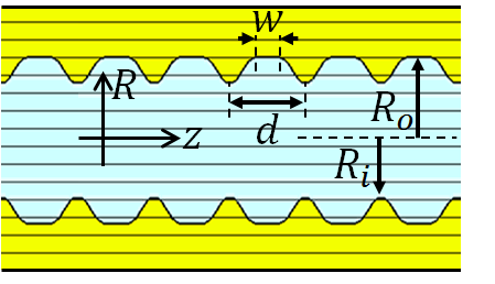
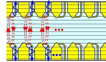
Figure 2: Longitudinal cross-sections of a SWS without (a) and with DPE (b).

As a proof of concept, we demonstrate the EPD-BWO regime by considering a conventional BWO operating at X-band whose SWS is shown in Fig. 2(a). The DPE is introduced by adding two wire loops in each unit cell, above and below as shown in Fig. 2, that couple to the azimuthal magnetic field and by Farady’s Law an electromotive force is generated that excites each coaxial waveguide, similarly to the way power is extracted from magnetrons (Ch. 10 in Ref. [7]). Simulations based on the particle in cell solver (PIC), implemented in CST Studio Suite, use a relativistic annular e-beam with dc voltage $V_{0}=600$ kV. The output signals and their corresponding spectra for both BWOs, with and without DPE, are shown in Fig. 3 where a self-standing oscillation frequency of 9.7 GHz is observed when the used beam dc current is $I_{0}=1740$ A for both cases. Details about the structure geometry and simulation settings are presented in Appendix C.

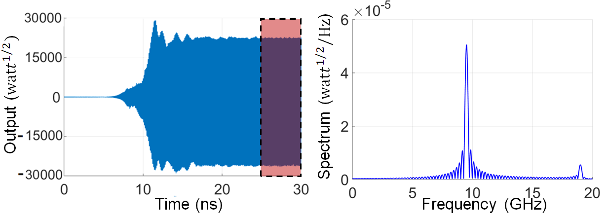
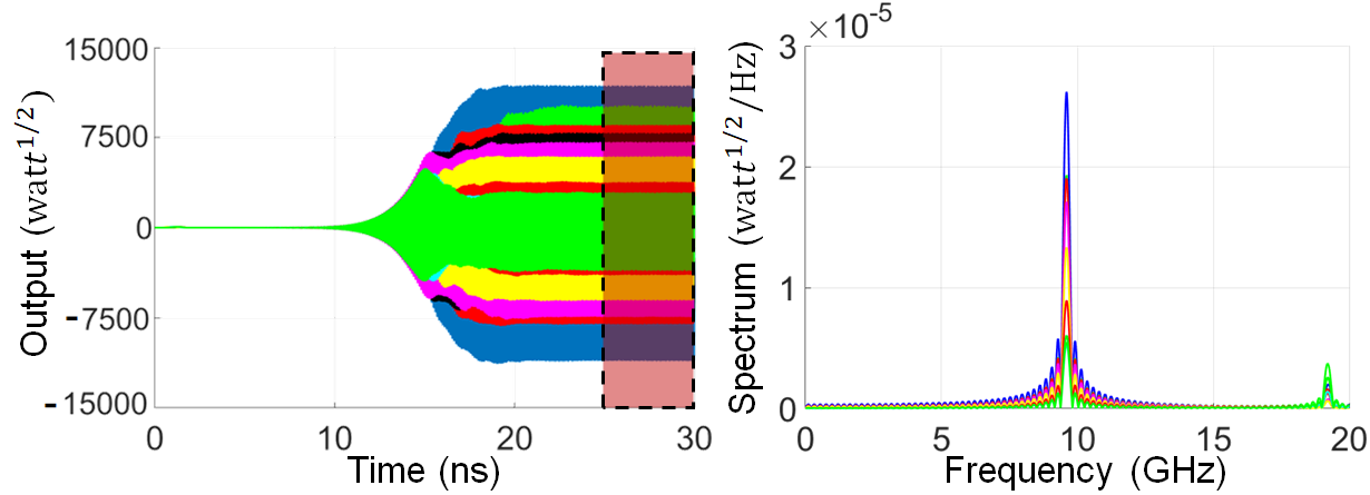
Figure 3: Output signals and their corresponding spectra for: (a) Conventional BWO where the output power is only extracted from one port as shown in Fig. 1(a). (b) EPD-BWO where power is extracted from multiple ports as shown in Fig. 1(b).

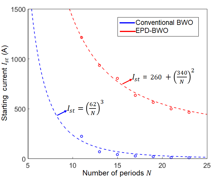
Figure 4: Scaling of starting e-beam current for oscillation in conventional BWO and EPD-BWO. Dashed lines represent fitting curves. The EPD-BWO shows a starting current trend that does not vanish for long SWS.

To assess the occurrence of an EPD we verify the unique scaling trend of the starting current in (5). Fig. 4 shows the starting current scaling trends for both conventional BWO and EPD-BWO based on PIC simulation results. The dashed lines represent fitting curves and the case of EPD-BWO shows very good fitting with 99% R-square. In comparison to a conventional BWO, the EPD-BWO is characterized by a starting current (threshold) that does not tend to zero as the SWS length increases, and a scaling that is a quadratic function of the inverse of the SWS length. The procedure to determine the starting current of oscillation using PIC simulations is presented in Appendix C.

We compare the RF conversion power efficiency (RF output power over dc e-beam power) of the conventional BWO with that of the EPD-BWO in Fig. 5 for e-beam dc currents that exceed the starting current, assuming the SWS has 11 unit-cells. The figure shows that the EPD-BWO has higher efficiency at higher level of output power compared to a conventional BWO with same dimensions. The results show that the EPD-BWO has a maximum efficiency of about 47% at about 0.5 GW output power (the sum of the power from each output in Fig. 1(b)). Instead, the conventional BWO has a maximum efficiency of about 33% at an output power level of about 0.27 GW. It is important to point out that the EPD-BWO has a higher threshold beam current to start oscillations compared to the conventional one which is in consistent with the theoretical results in [5] and with the requirement of generating higher power levels.

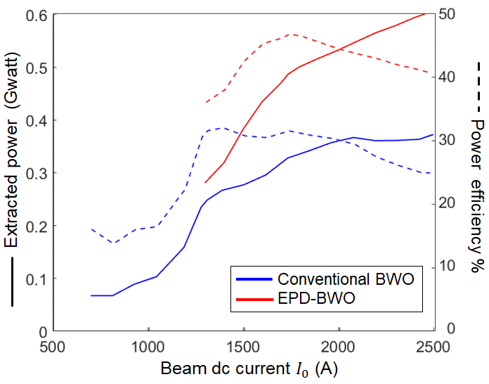
Figure 5: Comparison between the efficiency of a conventional BWO and an EPD-BWO. The EPD-BWO shows improved efficiency at higher level of power generation compared to the conventional BWO.

IV Conclusion

In summary, the physical mechanism of an EPD in a hybrid system where a linear electron beam interacts with an electromagnetic mode has been demonstrated. The manifestation of such EPD is useful to conceive a new degenerate synchronous regime for BWOs that have a starting-oscillation current law that decreases quadratically to a given fixed value for long waveguide interaction lengths; as a consequence PIC simulations show higher efficiency and much higher output power than a standard BWO. The unique quadratic threshold scaling law demonstrates the EPD-based synchronization phenomenon compared to that in a standard BWO that has a starting-oscillation current law that vanishes cubically for long waveguide interaction lengths.

V Acknowledgment

This material is based upon work supported by the Air Force Office of Scientific Research award number FA9550-18-1-0355. The authors are thankful to DS SIMULIA for providing CST Studio Suite that was instrumental in this study.

Appendix A Second order EPD in a system made of an electromagnetic wave interacting with an electron beam’s charge wave

The interaction between an electron (e)-beam and an electromagnetic (EM) wave in a linear vacuum tube was theoretically studied by Pierce in [14]. Assuming wave eigenfunctions of the interactive system of infinite length in the form of $\phi(z,t)\propto e^{i\omega t-ikz}$, Pierce showed that the solutions of the linearized differential equations that govern the electron beam charges’ motion and continuity in presence of the slow wave structure (SWS) EM field yield four eigenmodes whose wavenumber dispersion is given by the characteristic equation [14, 15]

$$\begin{array}[]{c}D(\omega,k)=k^{4}-2\beta_{0}k^{3}+\left(\beta_{0}^{2}-\beta_{p}^{2}+\dfrac{I_{0}Z_{c}\beta_{p}\beta_{0}}{2V_{0}}\right)k^{2}\\ \ \ \ \ \ \ \ \ \ \ \ \ \ \ \ \ \ \ \ \ \ \ \ \ \ \ \ \ \ \ \ \ +2\beta_{0}\beta_{p}^{2}k-\beta_{0}^{2}\beta_{p}^{2}=0,\end{array}$$ (A.1)

Here $\beta_{0}=\omega/u_{0}$ is the unmodulated e-beam wavenumber, $u_{0}$ is the average velocity of the electrons, $V_{0}$ and $I_{0}$ are the e-beam equivalent dc voltage and dc current, respectively, and $\beta_{p}$ and $Z_{c}$ are the wavenumber and characteristic impedance, respectively, of the EM mode in the “cold” (i.e., without interacting with the e-beam) SWS. The dispersion equation in (A.1) has four root solutions. The four complex wavenumbers are the eigenvalues of the interactive (also called “hot”) system. A necessary condition to have a second order exceptional point of degeneracy (EPD) is to have two repeated eigenvalues, which means that at the EPD frequency $\omega=\omega_{e}$ the characteristic equation should have two repeated roots as

$$\begin{array}[]{c}D(\omega_{e},k)\propto(k-k_{e})^{2}\end{array}$$ (A.2)

where $k_{e}$ is the degenerate wavenumber. The relation in (A.2) is satisfied when [16]

$$\begin{array}[]{c}D(\omega_{e},k_{e})=0,\\ \partial_{k}D(\omega_{e},k)\Big{|}_{k=k_{e}}=0.\end{array}$$ (A.3)

Using the expression for $D(\omega,k)$ in (A.1), the two necessary EPD conditions in (A.3) are explicitly written as

$$\begin{array}[]{c}k_{e}^{4}-2\beta_{0}k_{e}^{3}+\left(\beta_{0}^{2}-\beta_{p}^{2}+\dfrac{I_{0}Z_{c}\beta_{p}\beta_{0}}{2V_{0}}\right)k_{e}^{2}\\ \ \ \ \ \ \ \ \ \ \ \ \ \ \ \ \ \ \ \ \ \ \ \ \ \ \ \ \ \ \ \ \ +2\beta_{0}\beta_{p}^{2}k_{e}-\beta_{0}^{2}\beta_{p}^{2}=0,\end{array}$$ (A.4)

$$4k_{e}^{3}-6\beta_{0}k_{e}^{2}+2\left(\beta_{0}^{2}-\beta_{p}^{2}+\dfrac{I_{0}Z_{c}\beta_{p}\beta_{0}}{2V_{0}}\right)k_{e}+2\beta_{0}\beta_{p}^{2}=0.$$ (A.5)

Note that the frequency dependency is in the terms $\beta_{0}=\omega/u_{0}$, $\beta_{p}$ and $Z_{c}$. The frequency dependency in the cold SWS terms $\beta_{p}$ and $Z_{c}$ depends on the waveguide geometry and they can be approximated using simple distributed circuit models in the neighborhood of the operative frequency. Using a simple transmission line circuit model that supports backward propagation, the distributed per-unit-length series impedance $Z$ and shunt admittance $Y$ are $\beta_{p}=\sqrt{-ZY}$ and $Z_{c}=\sqrt{Z/Y}$, respectively, as also discussed in Ref. [5]. The two square roots values of each physical parameter represent waves that propagate in opposite directions in the cold SWS, i.e., both $\beta_{p}$ and $-\beta_{p}$ are valid solutions because of reciprocity, where the root $\beta_{p}=\sqrt{-ZY}$ is taken as the principle square root (resulting in a positive real part) while the root of $Z_{c}=\sqrt{Z/Y}$ is taken as the secondary square root (resulting in a negative real part) as discussed in [20, 5].

We simplify the above two equations by first getting $Z_{c}\beta_{p}$ from (A.5) as

$$Z_{c}\beta_{p}=\dfrac{2V_{0}\left(k_{e}-\beta_{0}\right)\left(\beta_{p}^{2}+k_{e}\left(\beta_{0}-2k_{e}\right)\right)}{I_{0}\beta_{0}k_{e}},$$ (A.6)

which is then used in (A.4) to get $\beta_{p}^{2}$ as

$$\beta_{p}^{2}=\dfrac{k_{e}^{3}}{\beta_{0}}.$$ (A.7)

We then simplify (A.6) by inserting (A.7) in its right hand side to get

$$Z_{c}\beta_{p}=\dfrac{2V_{0}\left(k_{e}-\beta_{0}\right)^{3}}{I_{0}\beta_{0}^{2}}.$$ (A.8)

The conditions in (A.7) and (A.8) are constraints on the cold SWS’s circuit parameters $\beta_{p}$ and $Z_{c}$ to enable the an EPD, and are important to select what kind of SWS shall be chosen to ensure an EPD occurs at a given $(\omega_{e},k_{e})$.

The above equations can also be used to determine the EPD wavenumber of the hot SWS, i.e., the wavenumber of the degenerate mode in the interactive e-beam-EM system; from (A.7) one obtains

$$k_{e}=\sqrt[3]{\beta_{p}^{2}\beta_{0}}.$$ (A.9)

Then, using this $k_{e}$ expression in (A.8), we obtain

$$\left(\dfrac{\beta_{p}}{\beta_{0}}\right)^{2}=\left(\sqrt[3]{\dfrac{I_{0}Z_{c}\beta_{p}}{2V_{0}\beta_{0}}}+1\right)^{3}.$$ (A.10)

The above condition represents a constraint involving the operational frequency $\omega$, electron beam dc voltage$V_{0}$ and current $I_{0}$, and cold SWS circuit wavenumber $\beta_{p}$ and characteristic impedance $Z_{c}$ to have an EPD.

When distributed power extraction (DPE) occurs in the SWS, the propagation constant and characteristic impedance of the “cold” EM mode (i.e., without coupling to the electron beam) are complex: $\beta_{p}=\beta_{pr}+i\beta_{pi}$ and $Z_{c}=Z_{cr}+iZ_{ci}$. The cold propagation constant imaginary part $\beta_{pi}$ accounts for power attenuation along the SWS due to the leakage of power out of the SWS. Note that $\beta_{pr}\beta_{pi}>0$ for a “backward” EM wave that is traveling in the cold SWS (we are using the $\exp(i\omega t)$ time dependency which implies that the EM modes propagates as $\exp(-i\beta_{p}z)$). Since the phase propagation constant $\beta_{pr}$ is positive, because it has to matche the electron beam effective wavenumber $\beta_{0}=\omega/u_{0}$, one has $\beta_{pi}>0$. Furthermore, for a backward wave with $\beta_{pr}>0$, one has $Z_{cr}<0$ since power travels along the $-z$ direction in the cold SWS. Therefore in the above formulas we have that $Z_{c}\beta_{p}=\left(Z_{cr}\beta_{pr}-Z_{ci}\beta_{pi}\right)+i\left(Z_{ci}\beta_{pr}+Z_{cr}\beta_{pi}\right)$ is complex.

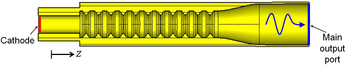
Figure 6: Longitudinal cross-sections of (a) the conventional BWO considered in this paper where the output power is extracted from the waveguide right end; (b) the EPD-BWO where the power is extracted in a distributed fashion to satisfy the EPD condition. The power is extracted using distributed wire loops (as an example) that are connected to coaxial waveguides on the top and bottom sides of the waveguide. This is just an example of DPE to provide the proof of concept of an EPD in a BWO; many other geometries are possible and the physical mechanism would be analogous to the one demosntrated in this paper.

Appendix B Electron beam dc current that satisfies the EPD condition

The electron beam current that satisfies the EPD condition is determined by rearranging (A.10) as

$$I_{0}=I_{0e}\equiv\dfrac{2V_{0}\beta_{0}}{Z_{c}\beta_{p}}\left(\left(\dfrac{\beta_{p}}{\beta_{0}}\right)^{2/3}-1\right)^{3}.$$ (B.1)

To satisfy the above condition, since the e-beam dc current $I_{0}$ is real valued, the imaginary part of the right hand side should vanish, i.e.,

$$\begin{array}[]{c}\mathrm{arg}\left(\dfrac{2V_{0}\beta_{0}}{Z_{c}\beta_{p}}\left(\left(\dfrac{\beta_{p}}{\beta_{0}}\right)^{2/3}-1\right)^{3}\right)=2n\pi,\end{array}n=\{0,\pm 1,..\}.$$ (B.2)

The propagation constant and characteristic impedance of the backward EM mode are complex, and the imaginary part $\beta_{pi}>0$ of the cold propagation constant accounts for distributed power extraction. Under the assumption that $0<\beta_{pi}\ll\beta_{pr}$ and $|Z_{ci}|\ll|Z_{cr}|$ and considering a backward propagating mode so that $\mathrm{Re}\left(Z_{c}\beta_{p}\right)<0$, it can be easily shown that $\left|\mathrm{Re}\left(Z_{c}\beta_{p}\right)\right|>\left|\mathrm{Im}\left(Z_{c}\beta_{p}\right)\right|$.

By assuming that the EPD point at $(\omega,k)=(\omega_{e},k_{e})$ is close to the synchronization point of the non interactive diagrams (that is $(\omega,\beta_{p})\approx(\omega,\beta_{0})$) , i.e., we impose that at $\omega=\omega_{e}$one has $\beta_{p}=\beta_{0}(1+\delta)$, where $\delta=\delta_{r}+i\delta_{i}$, and $\delta_{i}>0$ (because of losses and (DPE) in the cold SWS supporting the backward mode). Because we assume that both $|\delta_{r}|\ll 1$ and $\delta_{i}\ll 1$, the argument of the complex value in (B.2) is dominated by the latter term, i.e.,

$$\begin{array}[]{c}\mathrm{arg}\left(\dfrac{2V_{0}\beta_{0}}{Z_{c}\beta_{p}}\left(\left(\dfrac{\beta_{p}}{\beta_{0}}\right)^{2/3}-1\right)^{3}\right)\\ \ \ \ \ \ \ \ \ \ \ \ \ \ \ \ \ \ \ \ \ \ \ \ \ \ \ \ \ \ \ \ \ \approx\mathrm{\pi+3arg}\left(\left(\dfrac{\beta_{p}}{\beta_{0}}\right)^{2/3}-1\right).\end{array}$$ (B.3)

The cubic root in (B.3) has three solutions:

$$\begin{array}[]{cc}\left(\dfrac{\beta_{p}}{\beta_{0}}\right)^{2/3}\approx\left(1+\dfrac{2}{3}\delta\right)e^{i2m\pi/3},&m=\{0,1,2\}.\end{array}$$ (B.4)

Considering the cubic root solution with $m=0$, the argument in (B.3) is simplified to

$$\begin{array}[]{c}\mathrm{arg}\left(\dfrac{2V_{0}\beta_{0}}{Z_{c}\beta_{p}}\left(\left(\dfrac{\beta_{p}}{\beta_{0}}\right)^{2/3}-1\right)^{3}\right)\\ \ \ \ \ \ \ \ \ \ \ \ \ \ \ \ \ \ \ \ \ \ \ \ \ \ \ \ \ \ \ \ \ \approx\mathrm{\pi+3arg}\left(\dfrac{2}{3}\delta\right)\\ \ \ \ \ \ \ \ \ \ \ \ \ \ \ \ \ \ \ \ \ \ \ \ \ \ \ \ \ \ \ \ \ =\pi+3\tan^{-1}\left(\dfrac{\delta_{i}}{\delta_{r}}\right).\end{array}$$ (B.5)

By enforcing angle condition in (B.2) to (B.5) we obtain

$$\begin{array}[]{cc}\pi+3\tan^{-1}\left(\dfrac{\delta_{i}}{\delta_{r}}\right)=2n\pi,&n=0,\pm 1,...\end{array}$$ (B.6)

A relation between $\delta_{r}$ and $\delta_{i}$ is determined by solving (B.6) which finally yields three possible solutions

$$\delta_{i}=\begin{cases}\begin{array}[]{c}0\\ \sqrt{3}\delta_{r}\\ -\sqrt{3}\delta_{r}\end{array}\end{cases}.$$ (B.7)

We neglect the solution $\delta_{i}=0$ in (B.7) because the regime we are considering has DPE which implies that $\delta_{i}>0.$ Using the solution $\delta_{i}=\pm\sqrt{3}\delta_{r}$ in (B.1) will finally find the EPD current to be

$$I_{0e}\approx\dfrac{2V_{0}}{Z_{cr}}\left(\dfrac{2}{3}\left(\delta_{r}\pm i\sqrt{3}\delta_{r}\right)\right)^{3}=\dfrac{128}{81\sqrt{3}}\dfrac{V_{0}\delta_{i}^{3}}{(-Z_{cr})}$$ (B.8)

Therefore, the EPD condition is met by just tuning the e-beam dc current $I_{0}$ to a specific value which we call EPD e-beam current $I_{0e}$:

$$I_{0}=I_{0e}\approx\dfrac{128}{81\sqrt{3}}\dfrac{V_{0}}{\left(-Z_{cr}\right)}\dfrac{\beta_{pi}^{3}}{\beta_{0}^{3}}\bigg{|}_{\beta_{pr}=\beta_{0}}.$$ (B.9)

The other two solutions of the cubic root in (B.4) with $m=1$ and $m=2$ are discarded because they provide solutions for a purely real right hand side of Eq. (B.1) for $|\delta_{i}|>1$ and $\left|\delta_{r}\right|>1$, that contradict the initial assumption of $|\delta_{r}|\ll 1$ and $\delta_{i}\ll 1$. In summary, the EPD occurs when the e-beam current $I_{0}$ takes the value in (B.9).

Appendix C Full-wave simulations’ details

We demonstrate the EPD-BWO regime by taking a conventional BWO design operating at X-band shown in Fig. 6(a). The proposed EPD-BWO is shown is Fig. 6(b) where DPE is introduced using distributed wire loops that are connected to coaxial waveguides. The original SWS geometry shown in Fig. 7, is a circular copper waveguide with azimuthal symmetry and with inner and outer radii of $R_{i}$ = 11.5 mm and $R_{o}=16.5$ mm, respectively, and period $d=15$ mm. The surface corrugation of SWS in one period is described by a flat surface $R(z)=R_{o}$ for $0\leq z<w$, where $w=5$ mm, and a sinusoidal corrugated surfaces for the rest of the period described as $R(z)=(R_{o}+R_{i})/2+((R_{o}-R_{i})/2)\cos(2\pi(z-w)/(d-w))$ for $w\leq z<d$. The whole body of the BWO is made of copper with vacuum inside.

C-A Cold simulations - EM modes in the cold SWS

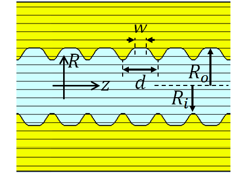
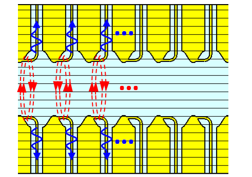
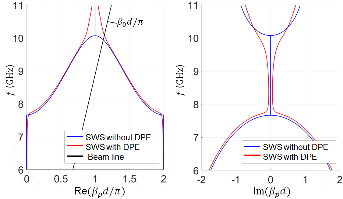
Figure 7: Details of the longitudinal cross-sections of a SWS without (a) and with DPE (b). (c) Dispersion of EM guided modes in the “cold” SWSs in (a) and (b), without (blue curve) and with (red curve) distributed power extraction (DPE), respectively. The dispersion shows the real and imaginary parts of the complex wavenumber. The non-zero imaginary part of wavenumber (red line) shows that the SWS in (b) exhibits distributed power extraction. The black line is the “beam line” described by $\beta_{0}=\omega/u_{0}$ , and the intersection point with the curve of $\beta_{pr}=\mathrm{Re}(\beta_{pr})$ represents the approximative syncronization point.

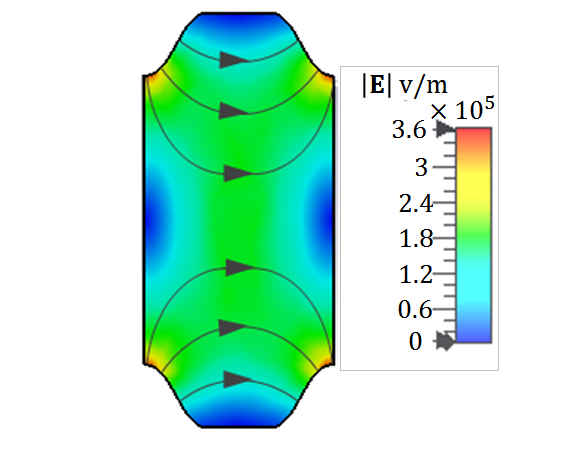
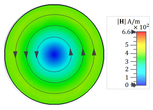
Figure 8: Field distribution for the TM-like mode supported by the SWS in Fig. 7: (a) electric field on the longitudinal cross-section, and (b) magnetic field on the transverse cross-section. Fields are found with the mode solver of CST Studio Suite.

The DPE is introduced by adding two wire loops in each unit cell, above and below as shown in Fig. 7, that couple to the azimuthal magnetic field (shown in Fig. 8), and by Farady’s Law an electromotive force is generated that excites each coaxial waveguide, similarly to the way power is extracted from magnetrons (Ch. 10 in Ref. [7]). The coaxial cables have outer and inner radii equal to $2.57$ mm and $0.5$ mm, respectively, leading to a 98 ohm characteristic impedance. Figure 7 shows a comparison between the dispersion relation of the EMmodes in the two “cold” SWSs: one used in the conventional BWO in Fig. 7, and the other one used in the BWO with DPE in Fig. 7. The dispersion curves show only the EM mode that is TM-like, i.e., the one with an axial (longitudinal) electric field component, with electric and magnetic field distributions shown in 8. The dispersion curves in Fig 7 show that the EM mode in the cold SWS with DPE is a backward wave that has a propagation constant with non-zero imaginary part $\beta_{pi}$ at the frequency where the interaction with the e-beam occurs, i.e., at the point where the EM wave phase velocity $\omega/\beta_{pr}$ is synchronized to the velocity of electrons $u_{0}=0.88c$, where $c$ is the speed of light in vacuum. This means that the cold SWS in Fig. 7 is suitable for our design of a BWO with an EPD [6, 5]. An example of the dispersion of the complex-wavenumber modes in the interactive (“hot”) EM e-beam system with DPE has been shown in [6, 5] using the Pierce-based model revealing the occurrence of an EPD. The complex wavenumber dispersion relation in presence of DPE, shown in Fig 7, is obtained by using two multi-mode ports at the begin and end of a SWS unit-cell where each port has 30 modes (almost all evanescent) that sufficiently represent the first TM-like Floquet mode in the periodic SWS, while all the coaxial waveguides are matched to their characteristic impedance to absorb all the outgoing power. This is done using the Finite Element Frequency Domain solver implemented in CST Studio Suite by DS SIMULIA that calculates the scattering parameters of the unit cell, that have then been converted to a transfer matrix to get the SWS complex Floquet-Bloch modes following the same method in [21].

C-B Hot simulations - oscillation frequency and fields

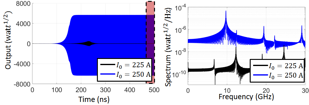
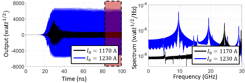
Figure 9: Output signal at the right-end waveguide port and its corresponding spectrum when the SWS has 11 unit-cells, at (blue) and below (black) the e-beam starting current for: (a) Conventional BWO and (b) EPD-BWO. The frequency spectrum shows that there is not self-standing oscillation at 9.7 GHz when the e-beam dc current is below the oscillation threshold, i.e., when the current is below $250$A for theconventional BWO, and below $1230$A for the EPD-BWO, but there is at these two e-beam current values, hence they are the starting currents for the two types of BWOs. It is important to stress that the figure shows only the ouput power at the right-end port of the EPD-BWO, and indeed the output value of the EPD-BWO is comparable to the one coming out of the conventional BWO. The total amount of power coming out of the EPD-BWO is much higher than the one of the conventional BWO when we consider all the other distributed ports, as shown in Fig. 5 of the main body of the paper.

Simulations based on the particle-in-cell (PIC) solver, implemented in CST Studio Suite, based on a relativistic annular e-beam with dc voltage of $V_{0}=600$ kV, inner and outer radii of $R_{ib}=9$ mm and $R_{ob}=10.3$ mm, respectively, and with dc axial magnetic field of 2.6 T to confine the electron beam. The cathode is modeled using the dc emission model with 528 uniform emission points. The full-wave simulation uses around 1.3M Hexahedral mesh cells to model the SWS.

We study the starting e-beam current for oscillation in both types of BWO (the conventional one, and the EPD-BWO in Fig. 6 by sweeping the e-beam current $I_{0}$ and monitoring the RF power and its spectrum of the waveguide output signal at the right end of the cylindrical waveguide. Using a SWS with 11 unit-cells we show in Fig. 9 the output power at the main port at the right end of the SWS when the e-beam current is just below and just above the threshold current. A self-standing oscillation frequency of 9.7 GHz is observed when the e-beam dc current $I_{0}$ for the conventional BWO is at or larger than than $250$A, while for the EPD-BWO, self-standing oscillations is observed for an e-beam current $I_{0}$ equal or greater than $1230$A. Such oscillations are not observed for smaller e-beam current, as for example $225$A for the conventional BWO and $1170$A for the EPD-BWO. Therefore we conclude that the the starting current of oscillation is approximately $250$A for the conventional BWO, and $1230$A for the EPD-BWO, when the SWS length is 11 periods.

Figure 10 shows the electric field distribution for the conventional BWO and the EPD-BWO when the e-beam dc current $I_{0}$ is $1750$ A, in both cases, for a SWS of 11 unit cells. The figure shows that ffor the conventional BWO the power is extracted only from the main port at the right end, whereas for EPD-BWO most of the power is extracted in a distributed fashion from the top and bottom coaxial waveguides, resulting in much high power and high efficiency as demonstrated in the main body of this paper.

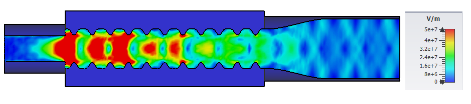
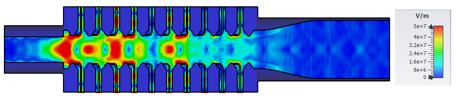
Figure 10: Electric field distribution in the SWS for: (a) conventional BWO and (b) EPD-BWO. The figure in (b) shows power extraction in distributed fashion from the coaxial waveguides.

References

- [1] M. V. Berry, “Physics of nonhermitian degeneracies,” Czechoslovak Journal of Physics, vol. 54, no. 10, pp. 1039–1047, 2004.
- [2] C. M. Bender and S. Boettcher, “Real spectra in non-Hermitian Hamiltonians having PT symmetry,” Physical Review Letters, vol. 80, no. 24, p. 5243, 1998.
- [3] S. Klaiman, U. Günther, and N. Moiseyev, “Visualization of branch points in p t-symmetric waveguides,” Physical review letters, vol. 101, no. 8, p. 080402, 2008.
- [4] M. Liertzer, L. Ge, A. Cerjan, A. Stone, H. E. Türeci, and S. Rotter, “Pump-induced exceptional points in lasers,” Physical Review Letters, vol. 108, no. 17, p. 173901, 2012.
- [5] T. Mealy, A. F. Abdelshafy, and F. Capolino, “Exceptional point of degeneracy in backward-wave oscillator with distributed power extraction,” arXiv preprint arXiv:1904.12946, 2019.
- [6] T. Mealy, A. F. Abdelshafy, and F. Capolino, “Backward-wave oscillator with distributed power extraction based on exceptional point of degeneracy and gain and radiation-loss balance,” in 2019 International Vacuum Electronics Conference (IVEC), pp. 1–2, IEEE, 2019.
- [7] A. Gilmour, Principles of traveling wave tubes. Norwood, MA, USA: Artech House, 1994.
- [8] B. Levush, T. M. Antonsen, A. Bromborsky, W.-R. Lou, and Y. Carmel, “Theory of relativistic backward-wave oscillators with end reflectors,” IEEE transactions on plasma science, vol. 20, no. 3, pp. 263–280, 1992.
- [9] H. R. Johnson, “Backward-wave oscillators,” Proceedings of the IRE, vol. 43, no. 6, pp. 684–697, 1955.
- [10] S. Chen, K. Chu, and T. Chang, “Saturated behavior of the gyrotron backward-wave oscillator,” Physical review letters, vol. 85, no. 12, p. 2633, 2000.
- [11] L. D. Moreland, E. Schamiloglu, W. Lemke, S. Korovin, V. Rostov, A. Roitman, K. J. Hendricks, and T. Spencer, “Efficiency enhancement of high power vacuum bwo’s using nonuniform slow wave structures,” IEEE Transactions on Plasma Science, vol. 22, no. 5, pp. 554–565, 1994.
- [12] Z.-H. Li, “Investigation of an oversized backward wave oscillator as a high power microwave generator,” Applied Physics Letters, vol. 92, no. 5, p. 054102, 2008.
- [13] J. Zhang, H.-H. Zhong, Z. Jin, T. Shu, S. Cao, and S. Zhou, “Studies on efficient operation of an x-band oversized slow-wave HPM generator in low magnetic field,” IEEE Transactions on Plasma Science, vol. 37, no. 8, pp. 1552–1557, 2009.
- [14] J. Pierce, “Waves in electron streams and circuits,” Bell System Technical Journal, vol. 30, no. 3, pp. 626–651, 1951.
- [15] P. A. Sturrock, “Kinematics of growing waves,” Physical Review, vol. 112, no. 5, p. 1488, 1958.
- [16] G. W. Hanson, A. B. Yakovlev, M. A. Othman, and F. Capolino, “Exceptional points of degeneracy and branch points for coupled transmission lines—Linear-algebra and bifurcation theory perspectives,” IEEE Transactions on Antennas and Propagation, vol. 67, no. 2, pp. 1025–1034, 2019.
- [17] A. Welters, “On explicit recursive formulas in the spectral perturbation analysis of a jordan block,” SIAM Journal on Matrix Analysis and Applications, vol. 32, no. 1, pp. 1–22, 2011.
- [18] A. Seyranian, O. Kirillov, and A. Mailybaev, “Coupling of eigenvalues of complex matrices at diabolic and exceptional points,” Journal of Physics A: Mathematical and General, vol. 38, no. 8, pp. 1723–1740, 2005.
- [19] L. Walker, “Starting currents in the backward-wave oscillator,” Journal of Applied Physics, vol. 24, no. 7, pp. 854–859, 1953.
- [20] R. W. Ziolkowski and E. Heyman, “Wave propagation in media having negative permittivity and permeability,” Physical review E, vol. 64, no. 5, p. 056625, 2001.
- [21] M. A. Othman, V. A. Tamma, and F. Capolino, “Theory and new amplification regime in periodic multimodal slow wave structures with degeneracy interacting with an electron beam,” IEEE Transactions on Plasma Science, vol. 44, no. 4, pp. 594–611, 2016.