Investigating the physical conditions in extended system hosting mid-infrared bubble N14

Abstract

To observationally explore physical processes, we present a multi-wavelength study of a wide-scale environment toward l = 13$\arcdeg$.7–14$\arcdeg$.9 containing a mid-infrared bubble N14. The analysis of ¹²CO, ¹³CO, and C¹⁸O gas at [31.6, 46] km s^-1 reveals an extended physical system (extension $\sim$59 pc $\times$ 29 pc), which hosts at least five groups of the ATLASGAL 870 $\mu$m dust clumps at d $\sim$3.1 kpc. These spatially-distinct groups/sub-regions contain unstable molecular clumps, and are associated with several Class I young stellar objects (mean age $\sim$0.44 Myr). At least three groups of ATLASGAL clumps associated with the expanding H ii regions (including the bubble N14) and embedded infrared dark clouds, devoid of the ionized gas, are found in the system. The observed spectral indices derived using the GMRT and THOR radio continuum data suggest the presence of non-thermal emission with the H ii regions. High resolution GMRT radio continuum map at 1280 MHz traces several ionized clumps powered by massive B-type stars toward N14, which are considerably young (age $\sim$10³–10⁴ years). Locally, early stage of star formation is evident toward all the groups of clumps. The position-velocity maps of ¹²CO, ¹³CO, and C¹⁸O exhibit an oscillatory-like velocity pattern toward the selected longitude range. Considering the presence of different groups/sub-regions in the system, the oscillatory pattern in velocity is indicative of the fragmentation process. All these observed findings favour the applicability of the global collapse scenario in the extended physical system, which also seems to explain the observed hierarchy.

1. Introduction

It has been well accepted that molecular gas converts into young stellar objects (YSOs) of different masses (including massive OB stars ($\gtrsim$ 8 M_⊙)) and their clusters in a giant molecular cloud (GMC), where several complex physical processes may operate. However, the mechanisms responsible for the birth of young stellar clusters and massive stars are still incompletely understood (Zinnecker & Yorke, 2007; Tan et al., 2014). The study of a GMC allows to explore the ongoing star-formation mechanisms, such as global gravitational contraction (Hartmann et al., 2012, and references therein), triggered star formation scenarios (i.e., “globule squeezing”, “collect and collapse”, and “cloud-cloud collision (CCC)”; Elmegreen, 1998). Such study requires the knowledge of the physical conditions in promising massive star-forming sites (e.g., H ii regions) associated with a GMC, which can be inferred through the analysis of the multi-wavelength data. In this context, the present paper deals with an extended and a single physical system hosting several massive star-forming regions, which are situated toward l = 13$\arcdeg$.7–14$\arcdeg$.9 and b = $-$0$\arcdeg$.5–+0$\arcdeg$.1. This extended physical system located in the Galactic arm(s) is identified via the reliable information of distance and radial velocity ($V_{\mathrm{lsr}}$) of its different sub-regions, which helps to disentangle the target system against its background and foreground clouds.

Figure 1a shows the APEX Telescope Large Area Survey of the Galaxy (ATLASGAL; beam size $\sim$19$\farcs$2; Schuller et al., 2009) 870 $\mu$m dust continuum map covering the wide-scale area ($\sim$1$\arcdeg$.2 $\times$ 0$\arcdeg$.6) around the mid-infrared (MIR) bubble N14. The ATLASGAL map is also overlaid with 53 ATLASGAL clumps (taken from Urquhart et al., 2018). All these clumps are traced in a velocity range of [34.5, 43] km s^-1, and are located at a single distance of $\sim$3.1 kpc (Urquhart et al., 2018). The spatial distribution of these clumps has enabled us to find out an extended physical system. Based on the visual inspection, one can also arbitrarily depict at least five groups of clumps (i.e., group1, group2, group3, group4, and group5) in Figure 1a, which are indicated by broken curves. The MIR bubble N14 has been characterized as a complete or closed ring with an average radius and thickness of 1^′.22 and 0^′.38, respectively (Churchwell et al., 2006; Dewangan and Ojha, 2013; Yan et al., 2016). The bubble N14 also contains the ionized emission at its center (e.g., Dewangan and Ojha, 2013). Using the Multi-Array Galactic Plane Imaging Survey (MAGPIS; beam size $\sim$6^′′; Helfand et al., 2006) radio continuum flux at 20 cm of the bubble N14, Beaumont and Williams (2010) computed the Lyman continuum photons ($\log{N_{\mathrm{uv}}}$) to be 48.36 (see also Dewangan and Ojha, 2013), which is explained by a single O9V–O8.5V star (Panagia, 1973) or a single O7.5V–O8V star (Martins et al., 2005) or at least six O9.5V stars (Beaumont and Williams, 2010). In addition to the bubble N14, some other previously known sources (such as, G014.194$-$00.194, G14.427$-$00.075HII, G14.47$-$0.20, IRAS 18141$-$1615, and G14.71$-$0.19) are also labeled in Figure 1a. Figure 1b displays the overlay of the MAGPIS 20 cm continuum emission contours on the ATLASGAL map at 870 $\mu$m. In the direction of at least three groups of clumps (i.e., group2, group3, and group4 in Figure 1a), the MAGPIS 20 cm contours reveal the presence of H ii regions powered by massive OB stars.

However, the formation processes of the selected different groups of clumps as well as massive OB stars are yet to be investigated in the extended physical system (see Figure 1a). No attempt is made to examine the velocity structure of molecular gas and the identification of YSOs toward the entire selected longitude range. Such analysis is required for exploring the ongoing star formation mechanisms in the extended physical system containing several embedded clumps and H ii regions. It also helps us to observationally understand the origin of the large-scale configuration/system toward l = 13$\arcdeg$.7–14$\arcdeg$.9. In this context, a multi-wavelength approach is adopted in this paper, which is a very useful and effective utility to gain the quantitative and qualitative physical information in the target site. The present work is benefited with the existing large-scale FOREST Unbiased Galactic plane Imaging survey with the Nobeyama 45-m telescope (FUGIN; Umemoto et al., 2017) molecular line data (i.e., ¹²CO, ¹³CO, and C¹⁸O) along with the Spitzer and Herschel infrared maps. New radio continuum maps observed by Giant Metrewave Radio Telescope (GMRT) facility are also presented toward the MIR bubble N14.

This paper is arranged as follows. Section 2 presents the details of the adopted data sets in this paper. Section 3 provides new outcomes derived using a multi-wavelength approach in the selected longitude range. The discussion of the observational outcomes is presented in Section 4. Finally, Section 5 gives the summary of the major findings obtained in this work.

2. Data and analysis

The present paper utilizes the existing multi-wavelength data sets obtained from various large-scale surveys (see Table 1). The selected target area ($\sim$1$\arcdeg$.2 $\times$ 0$\arcdeg$.6 (or $\sim$65 pc $\times$ 32.5 pc); centered at $l$ = 14$\arcdeg$.3; $b$ = $-$0$\arcdeg$.2) in this paper is presented in Figure 1a. The ¹²CO(J =1$-$0), ¹³CO(J =1$-$0), and C¹⁸O(J =1$-$0) line data were obtained from the FUGIN survey, and are calibrated in main beam temperature ($T_{\mathrm{mb}}$) (Umemoto et al., 2017). The typical rms noise level ($T_{\mathrm{mb}}$) is $\sim$1.5 K, $\sim$0.7 K, and $\sim$0.7 K for ¹²CO, ¹³CO, and C¹⁸O lines, respectively (Umemoto et al., 2017). To improve sensitivities, each FUGIN molecular line data cube is smoothened with a Gaussian function having half power beam width of 35^′′. Additionally, in the direction of the bubble N14, our unpublished GMRT radio continuum maps are also examined in this work.

Radio continuum observations at 610 and 1280 MHz were performed with the GMRT facility on 2012 December 28 (Proposal Code: 23$\_$054; PI: L. K. Dewangan). The GMRT data were reduced using the Astronomical Image Processing System (AIPS) package, and the detailed reduction procedures can be found in Mallick et al. (2012, 2013). We flagged out bad data from the UV data by multiple rounds of flagging using the tvflg task of the AIPS. After several rounds of ‘self-calibration’, the final maps at 610 and 1280 MHz were produced with the synthesized beams of 5^′′.6 $\times$ 5^′′.2 and 6^′′ $\times$ 6^′′, respectively. In general, due to the Galactic background emission, the antenna temperature of the sources located toward the Galactic plane is expected to be increased. It is found more severe in the GMRT low frequency bands (i.e., 610 MHz), where the contribution from the background emission is generally much higher compared to the 1280 MHz band. More detailed description concerning the system temperature correction can be found in Baug et al. (2015, and references therein). Such correction is also applied to the GMRT 610 MHz data, before performing any scientific analysis. The final rms sensitivities of both the maps at 610 and 1280 MHz are $\sim$1 mJy beam^-1. The unit of brightness in Jy beam^-1 is adopted in this paper. However, the conversion from Jy beam^-1 to Jy sr^-1 is Jy beam${}^{-1}\times(\frac{\theta}{206265})^{2}\times\frac{\pi}{4\ln{2}}$= Jy sr^-1, where $\theta$ is the beam size in arcseconds.

Table 1Table provides the list of different surveys adopted in this paper.

Survey	band/line(s)	Resolution ($\arcsec$)	Reference
Multi-Array Galactic Plane Imaging Survey (MAGPIS)	20 cm	$\sim$6	Helfand et al. (2006)
The HI/OH/Recombination line survey of the inner Milky Way (THOR)	1–2 GHz	$\sim$25	Beuther et al. (2016)
GMRT observations (Proposal Code: 23$\_$054)	610 MHz, 1280 MHz	$\sim$5–6	PI: L. K. Dewangan
FUGIN survey	12CO, 13CO, C18O (J = 1–0)	$\sim$20	Umemoto et al. (2017)
APEX Telescope Large Area Survey of the Galaxy (ATLASGAL)	870 $\mu$m	$\sim$19.2	Schuller et al. (2009)
Herschel Infrared Galactic Plane Survey (Hi-GAL)	70–500 $\mu$m	$\sim$5.8–37	Molinari et al. (2010a)
Spitzer MIPS Inner Galactic Plane Survey (MIPSGAL)	24 $\mu$m	$\sim$6	Carey et al. (2005)
Spitzer Galactic Legacy Infrared Mid-Plane Survey Extraordinaire (GLIMPSE)	3.6–8.0 $\mu$m	$\sim$2	Benjamin et al. (2003)

3. Results

In the selected target area, the multi-wavelength data sets are analyzed to study the distribution of molecular gas, YSOs, embedded clumps, H ii regions, dust temperature as well as velocity structure.

3.1. Extended physical system hosting H ii regions

In the target longitude range (i.e., l = 13$\arcdeg$.7–14$\arcdeg$.9), different groups of the ATLASGAL 870 $\mu$m dust continuum clumps (at $V_{\mathrm{lsr}}$ range $\sim$[34.5, 43] km s^-1) are presented in Section 1, and are labeled in Figure 1a. In the direction of some of these ATLASGAL groups, the radio continuum emission is observed (see Figure 1b). The dust continuum emission at 870 $\mu$m may depict cold dust, while the ionized gas is traced by the radio continuum emission. As highlighted earlier, the extended physical system hosts several embedded clumps and H ii regions powered by massive OB stars. Hence, Figure 1b helps us to examine the spatial association between the dust clumps and the ionized gas in the system.

In Figure 1b, we have marked the positions of the radio continuum sources (for l $>$ 14$\arcdeg$.3) from the THOR survey (Bihr et al., 2016; Wang et al., 2018), which are shown by hexagons and pentagons. The THOR radio sources are detected toward the ATLASGAL clumps and the MAGPIS radio continuum emission. Each THOR radio source has spectral index ($\alpha$) value, which is defined as $F_{\nu}$ $\propto$ $\nu^{\alpha}$. Here, $\nu$ is the frequency of observation, and $F_{\nu}$ is the corresponding observed flux density. The spectral indices of THOR radio sources are derived using the radio peak fluxes at 1.06, 1.31, 1.44, 1.69, 1.82, and 1.95 GHz (e.g., Bihr et al., 2016). Note that the areas around the bubble N14 are not observed in the THOR survey. THOR sources with $\alpha$ $<$ 0 are shown by hexagons, while pentagons indicate THOR sources with $\alpha$ $>$ 0. These sources are G14.779$-$0.333 ($\alpha$ $\sim$2.25), G14.457$-$0.185 ($\alpha$ $\sim$0.58), G14.477$-$0.005 ($\alpha$ $\sim-0$.097), G14.490+0.021 ($\alpha$ $\sim-0$.026), G14.598+0.019 ($\alpha$ $\sim-$0.042), G14.668+0.013 ($\alpha$ $\sim-$0.599), G14.390$-$0.021 ($\alpha$ $\sim-$0.074), and G14.440$-$0.056 ($\alpha$ $\sim-$0.344). In general, the positive and negative values of $\alpha$ allow us to distinguish the thermal and non-thermal radio continuum emission in a given massive star-forming region, respectively. A positive or near zero spectral index refers to thermally emitting sources (Bihr et al., 2016). For example, supernova remnants (SNR) display non-thermal emission with $\alpha$ $\approx$ $-$0.5, while a steeper $\alpha$ $\approx$ $-$1 is expected in extragalactic objects (e.g., Rybicki & Lightman, 1979; Longair, 1992; Bihr et al., 2016). Based on the radio morphology, all the selected 8 THOR radio sources appear to be Galactic H ii regions. Six out of 8 THOR radio sources show $\alpha$ $<$ 0, suggesting the non-thermal radio continuum emission, and the remaining 2 THOR sources exhibit thermal radio continuum emission (or free-free emission).

In the catalog of ATLASGAL clumps (e.g., Urquhart et al., 2018), one can obtain the integrated flux and effective radius ($R_{\mathrm{c}}$) of each ATLASGAL clump as well as other parameters, such as distance, $V_{\mathrm{lsr}}$, dust temperature ($T_{\mathrm{d}}$), bolometric luminosity ($L_{\rm bol}$), clump mass ($M_{\mathrm{clump}}$), and H₂ column density ($N(\mathrm{H}_{2})$). Table 2 lists the positions and physical parameters of all these clumps. Additionally, we have also included the average volume density ($n_{\mathrm{H}_{2}}$ = 3$M_{\mathrm{clump}}$/(4$\pi$$R_{\mathrm{clump}}^{3}$$\mu_{\rm H_{2}}m_{\rm H}$)) of each clump in the table. In the calculation, we assume that each clump has a spherical geometry. The mean molecular weight $\mu_{\rm H_{2}}$ is adopted to be 2.8, and $m_{\rm H}$ is the mass of an hydrogen atom.

Figure 1c presents a plot of $V_{\mathrm{lsr}}$ of 53 ATLASGAL clumps vs. Galactic longitude range of l = 0$\arcdeg$ – 35$\arcdeg$. The locations of various spiral arms (i.e., near and far sides of the Sagittarius, Scutum, and Norma arms) of the Milky Way (from Reid et al., 2016) are also marked in Figure 1c. This analysis suggests that the cloud associated with the extended physical system is located toward the near sides of the Scutum and Norma arms. In Figure 2, we present the observed ¹²CO, ¹³CO, and C¹⁸O spectra toward the selected target area. These profiles are obtained by averaging the selected target area as presented in Figure 1a. In Figure 2, we find three velocity peaks around 23, 40, and 60 km s^-1. The extended physical system, containing H ii regions (including the bubble N14), is associated with the velocity component around 40 km s^-1, and is well depicted in a velocity range of [31.6, 46] km s^-1. Note that the observed velocities of all the selected ATLASGAL clumps are well fallen within this velocity range. This exercise also indicates that the extended physical system is not physically associated with other two velocity components around 23 and 60 km s^-1, which are not examined in this paper.

To display five groups of clumps, Figure 3a shows the positions of 53 ATLASGAL clumps at 870 $\mu$m using different symbols (i.e., up down triangles (group1), circles (group2), squares (group3), triangles (group4), and stars (group5)). The sites N14, G014.194$-$00.194, G14.427$-$00.075HII (and G14.47$-$0.20), G14.71$-$0.19 are seen toward group2, group3, group4, and group5, respectively. Figure 3b shows the distribution of $V_{\mathrm{lsr}}$ of 53 clumps against Galactic longitude. We find a noticeable velocity spread toward all the ATLASGAL groups (except group1), which is further explored using the molecular line data in Section 3.2. In Figure 3c, we display the distribution of the dust temperatures of clumps against the Galactic longitude, showing a dust temperature range of $\sim$8–34 K. In the group3 and group5, the clumps are found with $T_{\mathrm{d}}$ $<$ 15 K. In the direction of the bubble N14, the clumps associated with the group2 have $T_{\mathrm{d}}$ $>$ 25 K. One can find the masses and bolometric luminosities of the clumps associated with different ATLASGAL groups in Figures 3d and 3e, respectively. All the ATLASGAL groups (except group1 and group5) have clumps with $L_{\rm bol}$ $>$ 10³ L_⊙. In each group, at least two dense clumps (with $n_{\mathrm{H}_{2}}$ $>$10⁵ cm^-3) are found (see Table 2).

3.2. Kinematics of molecular gas

To study the distribution of molecular gas, the integrated FUGIN ¹²CO, ¹³CO, and C¹⁸O intensity maps are presented in Figures 4a, 4b, and 4c, respectively. In each intensity map, the molecular gas is integrated over a velocity range of [31.6, 46] km s^-1 (see also Figure 2). In the direction of the extended physical system, the distribution of molecular gas allows us to infer the existence of a GMC (extension $\sim$59 pc $\times$ 29 pc), which contains several dense regions traced using the C¹⁸O gas. In Figure 4b, a shell-like feature is highlighted by a broken ellipse, and is prominently seen in the ¹³CO map. Using the C¹⁸O line data, we have selected 11 molecular clumps in the direction of the bubble N14 (see three clumps in ATLASGAL group2), G014.194$-$00.194 (see seven clumps in ATLASGAL group3), and G14.427$-$00.075 (see one clump in ATLASGAL group4) (see squares in Figure 4c). Using the zoomed-in maps of C¹⁸O, Figures 5a, 5b, and 5c show the position(s) of the selected molecular clump(s) in the direction of group2, group3, and group4, respectively (see also Table 3). In Figure 6, we display the integrated ¹³CO velocity channel maps (at intervals of 1 km s^-1), revealing several clumpy regions in the GMC. In each velocity panel, the location of the bubble N14 is highlighted by a radio continuum contour. The shell-like feature is also marked in two velocity channel panels by a broken ellipse.

Using the optically thin C¹⁸O line data, the total molecular masses ($M_{\mathrm{mc}}({\mathrm{H}_{2}})$) and the virial masses ($M_{\mathrm{vir}}$) for the molecular clumps highlighted in Figures 4c and 5 are estimated. For the calculations, we have used the procedures and equations given in Dewangan et al. (2019) (see also Mangum & Shirley, 2016; Frerking et al., 1982; MacLaren et al., 1988, for equations). Adopting the values of mass and clump diameter for each molecular clump, the mean number density ($\bar{n}$) is also estimated. The derived physical parameters are tabulated in Table 3, which shows that all of these molecular clumps are massive ($>$10³ M_⊙) and dense ($>$10⁴ cm^-3). One can notice that the value of $M_{\mathrm{vir}}$ is calculated for the case of a spherically symmetric clump with a constant density, no external pressure, and no magnetic field. Our calculations enable us to determine the ratio of $M_{\mathrm{mc}}$ and $M_{\mathrm{vir}}$ for all the selected molecular clumps (see Table 3). Note that the uncertainties of both mass estimates are the combinations of several factors (e.g., Dewangan et al., 2019), some of which are unknown (such as, clump density profiles, the C¹⁸O excitation temperature etc.). We can consider an uncertainty in the mass calculation to be typically $\sim$20% and at largest $\sim$50%. Taking into account a value of $\sim$50% for both mass uncertainties, one could conclude that at least five of the eleven C¹⁸O clumps (two in the group2, two in the group3 and one in the group4) with $M_{\mathrm{mc}}$/$M_{\mathrm{vir}}$ $\geq$ 2 should be unstable. It implies that these molecular clumps are unstable against gravitational collapse.

Figures 7a, 7b, and 7c display the longitude-velocity maps of ¹²CO, ¹³CO, and C¹⁸O, respectively. These molecular emissions exhibit a large spread in velocities over a range of $\sim$10–12 km s^-1 over the entire physical system. In the direction of the extended physical system, continuous velocity structures are seen, where velocity gradients are also evident. The velocity appears to be oscillating along the longitude in all the position-velocity maps. Overall, the analysis of molecular gas confirms the spatial and velocity connections of all the selected groups. It indicates that due to some physical processes, the extended physical system breaks into smaller groups in a hierarchical manner (see Section 4 for more details).

In the integrated molecular map of ¹³CO, we have highlighted a shell-like feature toward l = 14$\arcdeg$.3–14$\arcdeg$.5 or the site G14.427$-$00.075HII. In this selected longitude direction or the site G14.427$-$00.075HII, an arc-like feature is seen in velocity (see a dashed box in Figures 7a, 7b, and 7c). In Figure 7d, we display a zoomed-in view of the cloud associated with the site G14.427$-$00.075HII. To further examine the velocity structure toward the site G14.427$-$00.075, Figures 7e and 7f present the latitude-velocity and longitude-velocity maps of ¹³CO, respectively. The latitude-velocity map clearly reveals the arc-like feature in the velocity space, which is also seen in Figure 7f (see a broken curve in Figures 7e and 7f). Hence, both the position-velocity maps favour the presence of an expanding H ii region toward the site G14.427$-$00.075. Earlier, the semi-ring-like or C-like or arc-like structure in velocity has been observed in massive star-forming regions (such as, Orion nebula (Wilson et al., 2005), Perseus molecular cloud (Arce et al., 2011), W42 (Dewangan et al., 2015), S235 (Dewangan et al., 2016a)). Using a modeling of expanding bubbles in a turbulent medium, Arce et al. (2011) proposed that an expanding shell associated with the cloud should be responsible for the semi-ring-like or C-like structure in velocity. Considering the signature of the expanding H ii region, the observed radio continuum emission as well as the extended temperature structures, we suggest the impact of massive star(s) associated with the site G14.427$-$00.075HII to its vicinity.

The noticeable velocity gradient (i.e., $\sim$1 km s^-1 pc^-1) is also clearly seen toward the bubble N14 (see a solid white line in Figure 7c), where the extended and spherical-like temperature feature is evident (see Figure 9a). Earlier, Yan et al. (2016) reported the molecular maps toward the bubble N14 using different molecular lines (see Figure 5 in their paper). Sherman (2012) published the observational data at 3.3 mm continuum and several molecular lines toward the bubble N14. Based on the N₂H⁺ line data, they pointed out that the bubble N14 is expanding into a very inhomogeneous cloud. Our findings favour this interpretation.

In order to highlight the oscillatory-like velocity pattern, in Figures 8a and 8b, an arbitrarily chosen curve is drawn in the longitude-velocity maps of ¹³CO. Figure 8a is the same as in Figure 7b, but the ¹³CO emission is shown for higher contour levels. In Figure 8b, the molecular emission is integrated over a small range of latitude (i.e., $-$0$\arcdeg$.228 to $-$0$\arcdeg$.065). In this selected latitude range, most of the molecular emission is observed toward the extended physical system (see broken lines in Figure 8c). In addition to the oscillatory-like velocity pattern, in Figure 8b, velocity gradients are also evident toward the selected groups/sub-regions, as discussed above. In Figure 8c, we display the first moment map of C¹⁸O, showing the intensity-weighted mean velocity of the emitting gas. In the first moment map, one can clearly find noticeable velocity spread in the direction of the selected groups/sub-regions. We have also shown the distribution of the $V_{\mathrm{lsr}}$ of the ATLASGAL clumps and the locations of Galactic arms in Figure 8a. We also find the information of the NH₃ line-widths toward at least 10 ATLASGAL clumps (see red diamonds in Figure 8a and also Table 2) from Urquhart et al. (2018), which are used to compute the virial masses of the clumps. Based on the ratio of $M_{\mathrm{clump}}$ and $M_{\mathrm{vir}}$, we find that these clumps (with $M_{\mathrm{clump}}$ $>$ $M_{\mathrm{vir}}$) are unstable against gravitational collapse.

3.3. Temperature map, column density map, and embedded protostars

In Figures 9a and 9b, we have presented the Herschel temperature and column density ($N(\mathrm{H}_{2})$) maps (resolution $\sim$12^′′) of our selected target area, respectively. These maps were generated for the EU-funded ViaLactea project (Molinari et al., 2010b) using the Bayesian PPMAP method (Marsh et al., 2015, 2017), which was applied on the Herschel images at wavelengths of 70, 160, 250, 350 and 500 $\mu$m. In Figure 9a, the Herschel temperature map is also superimposed with the MAGPIS 20 cm continuum contour. Radio continuum emission or H ii regions are found toward the areas with a relatively warm dust emission ($T_{\mathrm{d}}$ $>$21 K). In the extended physical system, at least three highlighted sites (i.e., G14.71$-$0.19, G14.47$-$0.20, and G014.194$-$00.194) are associated with the areas of cold dust emission (i.e., $T_{\mathrm{d}}$ $\sim$16.5–18 K; see also Figure 1a). The most prominent feature in the Herschel temperature map is seen toward the bubble N14. The temperature structure of the bubble N14 is almost spherical, which is in agreement with the radio morphology. It seems that the feedback from massive stars (such as, stellar wind, ionized emission, and radiation pressure) might have heated the surroundings and is responsible for the extended temperature structure.

The column density map shows the distribution of materials with high column densities ($>$ 2.4 $\times$ 10²² cm^-2) toward the highlighted sites (e.g., N14, G014.194$-$00.194, G14.427$-$00.075HII (and G14.47$-$0.20), G14.71$-$0.19) in the extended physical system. Using the Spitzer 8.0 $\mu$m image, Herschel column density map, and Herschel temperature map, Figures 10a, 10b, and 10c display a zoomed-in view of the area hosting some highlighted sources (e.g., IRAS 18141$-$1615, G14.427$-$00.075HII, and G14.47$-$0.20), respectively. The positions of the THOR radio sources are marked in Figures 10a, 10b, and 10c. The MAGPIS 20 cm continuum contours are also overplotted on the Spitzer 8.0 $\mu$m image. The Spitzer image reveals extended bright emission as well as infrared dark clouds (IRDCs). The IRDCs are depicted as the absorption features against the Galactic background in the 8.0 $\mu$m image. The IRDCs are found with cold dust emission as well as high column density materials (see Figures 10a, 10b, and 10c). Previously, the extended emission at Spitzer 8.0 $\mu$m has been observed toward the bubble N14 (Churchwell et al., 2006; Dewangan and Ojha, 2013; Yan et al., 2016). In general, it is known that the Spitzer 8.0 $\mu$m band contains polycyclic aromatic hydrocarbon (PAH) features at 7.7 and 8.6 $\mu$m. Considering the extended warm dust emission, PAH features and molecular gas surrounding the ionized emission, one can infer the existence of photon dominant regions (PDRs) in the extended physical system. The PDRs are traced by the PAH emission, and indicate the molecular/ionized gas interface where one can expect the influence of UV radiation liberated by a nearby massive star.

To infer different sub-regions in the extended physical system, the clumpfind algorithm is adopted with the $N(\mathrm{H}_{2})$ of 2.4 $\times$ 10²² cm^-2 as an input parameter. At least 21 sub-regions are identified, which are also marked and labeled in Figure 11a. The total mass of each sub-region is estimated using an equation, $M_{area}=\mu_{\rm H_{2}}m_{\rm H}Area_{pix}\Sigma N(\mathrm{H}_{2})$, where $\mu_{\rm H_{2}}$ (= 2.8) is defined earlier, $Area_{pix}$ is the area subtended by one pixel (i.e., 6^′′/pixel), and $\Sigma N(\mathrm{H}_{2})$ is the total column density (see also Dewangan et al., 2017). In Table 4, the mass and the radius of each Herschel sub-region are listed. The masses of the Herschel sub-regions vary between 335 and 42975 M_⊙.

Figure 11b shows the distribution of the selected Class I YSOs (mean age $\sim$0.44 Myr; Evans et al., 2009) toward the Herschel sub-regions, tracing the early phases of star formation activities in the extended physical system (see white circles). In other words, star formation activities are traced toward all the groups of the ATLASGAL clumps. Previously, using the Spitzer 3.6–5.8 $\mu$m photometric data, Hartmann et al. (2005) and Getman et al. (2007) applied the infrared color conditions (i.e., [4.5]$-$[5.8] $\geq$ 0.7 mag and [3.6]$-$[4.5] $\geq$ 0.7 mag) to identify Class I YSOs in a given star-forming region. We have used this selection scheme to select Class I YSOs in the extended physical system. In this context, photometric magnitudes of point-like objects at 3.6–5.8 $\mu$m were obtained from the Spitzer GLIMPSE-I Spring’ 07 highly reliable catalog. In this work, we considered only objects with a photometric error of less than 0.2 mag in the selected Spitzer bands.

In Figure 11c, one can examine the distribution of ATLASGAL clumps at 870 $\mu$m toward the Herschel sub-regions. A majority of ATLASGAL clumps at 870 $\mu$m (see Table 2) are mainly found in the direction of four Herschel sub-regions (see IDs # h4, h5, h8, and h14 in Table 4; mass range: 5400–42975 M_⊙), where signposts of active star formation are investigated (see Figure 11c). Using the C¹⁸O line data, dense molecular clumps (see Table 3) are also identified toward the Herschel sub-regions (see IDs # h4, h5, and h8 in Table 4).

3.4. GMRT radio continuum maps

We find that the MAGPIS 20 cm continuum map reveals the compact radio continuum emission toward the bubble N14, while the diffuse radio emission is seen away from the bubble (see white contour in Figure 9a). To further explore the ionized emission, low-frequency radio continuum maps of the bubble N14 are examined in this paper. In Figures 12a and 12b, we display high-resolution GMRT radio continuum maps at 610 MHz (beam size $\sim$5^′′.56 $\times$ 5^′′.22) and 1280 MHz (beam size $\sim$6^′′), respectively. The GMRT 610 MHz continuum map is also superimposed with the 610 MHz continuum contour (see Figure 12a). In Figure 12b, the GMRT 1280 MHz continuum map is also overlaid with the 1280 MHz continuum contour. Figure 12c displays the overlay of the GMRT 1280 MHz continuum emission contours on the Spitzer 8.0 $\mu$m image. The spherical-like radio morphology observed in the GMRT maps is found well within the bubble boundary. In Figures 12a, 12b, and 12c, different color contours are used to show the inner radio morphology within the bubble N14.

Using the GMRT 1280 MHz continuum map, at least 17 radio clumps are identified toward the bubble N14, which are shown in Figure 12d (see a broken box in Figure 12b). In this analysis, the clumpfind algorithm (Williams et al., 1994) was employed. Adopting the similar procedures given in Dewangan et al. (2017), the Lyman continuum photons (see also Matsakis et al., 1976, for equation) and spectral type of each radio source are computed. In the calculation, we used a distance of $\sim$3.1 kpc, an electron temperature of 10⁴ K, and the models of Panagia (1973, see his Table 2). The analysis suggests that all the ionized clumps are powered by massive B-type stars. We have tabulated the derived physical properties of the ionized clumps (i.e., deconvolved effective radius of the ionized clump ($R_{\mathrm{HII}}$), total flux ($S{{}_{\nu}}$), Lyman continuum photons ($\log{N_{\mathrm{uv}}}$), dynamical age ($t_{\mathrm{dyn}}$), and radio spectral type) in Table 5. Using the equation given in Dyson & Williams (1980), we have computed the values of $t_{\mathrm{dyn}}$ for each radio clump (see Dewangan et al., 2017, for more details). The ages of all these radio clumps are found between $\sim$10³–10⁴ yr for an initial particle number density (n_i) of 10³ cm^-3, indicating that they are very young. Furthermore, the values of $S{{}_{\nu}}$ and $N_{\mathrm{uv}}$ are also computed for the entire extended spherical emission using the GMRT 1280 MHz continuum map. The integrated flux is estimated to be $S{{}_{\nu}}$ $\sim$3.54 Jy at 1280 MHz, which yields $\log{N_{\mathrm{uv}}}$ to be $\sim$ 48.42. It implies that the observed extended radio emission can be explained by a single ionizing star of spectral type O8.5V (e.g., Panagia, 1973). It is also in agreement with the analysis of the GMRT 610 MHz data (not presented here) as well as the previously reported value of $\log{N_{\mathrm{uv}}}$ (= 48.36; Beaumont and Williams, 2010).

In general, radio continuum data at low frequencies are very useful to trace the non-thermal emission in a given astrophysical object (e.g., De Becker, 2018). In order to infer the spectral indices of the radio clumps toward the bubble N14, the GMRT radio continuum maps at 610 and 1280 MHz are convolved to the same (lowest) resolution, and at least two radio clumps (i.e., clump A and clump B) are identified. Figures 13a and 13b show the radio spectral index plots of clump A and clump B, respectively. The spectral indices of the radio clumps are also labeled in Figures 13a and 13b. The positions of these clumps are also highlighted in Figure 12a (see clump A ($\alpha$ $\sim$$-$0.73) and clump B ($\alpha$ $\sim$$-$0.14)). This exercise indicates the presence of non-thermal emission in the bubble N14. Additionally, in the direction of l $>$ 13$\arcdeg$.4, we also find that several H ii regions or THOR radio sources show non-thermal emission. It has been reported that H ii regions powered by massive OB stars are normally associated with thermal emission (e.g., Wood & Churchwell, 1989; Kurtz, 2005; Sánchez-Monge et al., 2008, 2011; Hoare et al., 2012; Purcell et al., 2013; Wang et al., 2018; Yang et al., 2019). In the literature, we also find some examples of H ii regions (i.e., IRAS 17160$-$3707 (Nandakumar et al., 2016) and IRAS 17256$-$3631 (Veena et al., 2016)), which emit both thermal and non-thermal radiation. The observed non-thermal emission in H ii regions indicates the presence of relativistic electrons. More recently, it has been suggested that the non-thermal emission in H ii regions might be referred to synchrotron radiation from locally accelerated electrons restrained in a magnetic field (see Padovani et al., 2019, for more details).

4. Discussion

Based on the analysis of the molecular gas and the distribution of the ATLASGAL clumps, an extended physical system ($\sim$59 pc $\times$ 29 pc) is identified toward l = 13$\arcdeg$.7–14$\arcdeg$.9 containing the bubble N14. The system is found to host at least five groups or sub-regions. The spatial and velocity connections of these sub-regions are also found in the analysis of the molecular line data (see Section 3.2). Hence, the present work focuses to explore the physical processes responsible for the observed hierarchy in the extended physical system. These groups host unstable clumps (see Tables 2 and 3), and are associated with the C¹⁸O emission. These dense clumps are associated with Class I YSOs, which trace the early phase of star formation (see Section 3.3). Furthermore, some of the sub-regions (e.g., group2 and group4) harbor massive OB stars, and their associated H ii regions are found to be expanding in their surroundings (see Section 3.2). In the direction of the H ii regions, the extended structures in the Herschel temperature map are also found, illustrating the signatures of the impact of massive stars via their energetics (i.e., stellar wind, ionized emission, and radiation pressure). Hence, to explain the observed hierarchy, the application of “globule squeezing” and “collect and collapse” processes can be examined. These two processes are explained by the expanding H ii regions powered by massive stars (e.g., Elmegreen & Lada, 1977; Whitworth et al., 1994; Elmegreen, 1998; Deharveng et al., 2005; Dale et al., 2007; Bisbas et al., 2015; Walch et al., 2015; Kim et al., 2018; Haid et al., 2019, and references therein).

In general, the impact of a massive star can be studied with the knowledge of the pressure of an H ii region ($P_{HII}$), the radiation pressure ($P_{rad}$), and the stellar wind ram pressure ($P_{wind}$) (e.g., Dewangan et al., 2015, 2017). Based on the values of different pressure components, the influence of massive stars to their surroundings is found to be more significant upto a projected distance of a few parsecs (e.g., Dewangan et al., 2015, 2016b, 2017; Baug et al., 2019). Our observational results indicate that these processes might have influenced star formation activities locally in the extended physical system. However, these two processes may not explain the hierarchy extended upto about 59 pc in the selected target area.

In one of the theoretical models, the observed star formation can be explained by convergent gas flows (Ballesteros-Paredes et al., 1999; Heitsch et al., 2008; Vázquez-Semadeni et al., 2007) or the CCC process (e.g., Habe & Ohta, 1992). The model predicts that the convergence of streams of neutral gas can produce molecular clouds (e.g., Ballesteros-Paredes et al., 1999; Heitsch et al., 2008; Vázquez-Semadeni et al., 2007). With time, one also expects the merging/converging/collision of the molecular clouds. However, we do not find distinct multiple velocity components associated with the extended physical system. In Figure 8c, noticeable velocity spreads toward all the selected groups (except group5) are evident in the first moment map of C¹⁸O. In Sections 3.1 and 3.2, our observational results also show that the extended physical system is situated toward the near sides of the Scutum and Norma arms. Hence, locally, one cannot completely discard a triggered star formation scenario by convergent gas flows or the CCC process (e.g., Habe & Ohta, 1992).

In recent years, it has been suggested that star-forming clouds seem to be in a state of global gravitational contraction (e.g., Hartmann et al., 2012; Vázquez-Semadeni et al., 2019). It is also reported that the global collapse leads in a chaotic and hierarchical manner, yielding gravitationally driven fragmentation in star-forming molecular clouds (e.g., Burkert & Hartmann, 2004; Heitsch & Hartmann, 2008; Heitsch et al., 2009; Galván-Madrid et al., 2009; Peretto et al., 2013; Beuther et al., 2015; Liu et al., 2015, 2016b; Friesen et al., 2016; Jin et al., 2016; Hacar et al., 2017; Csengeri et al., 2017; Yuan et al., 2018; Jackson et al., 2019; Barnes et al., 2019; Vázquez-Semadeni et al., 2019). The modeling results based on the global hierarchical gravitational collapse in molecular clouds by Vázquez-Semadeni et al. (2019) indicate late birth of massive OB-stars and later loss of molecular gas feeding by feedback of massive stars. It also suggests that after the onset of global collapse, one can expect local collapse events in molecular clouds. Therefore, in the extended physical system, one can examine the observed hierarchy as the outcome of gravitational fragmentation (see the review article by Hennebelle & Falgarone, 2012).

In three-dimensional-models of molecular cloud formation in large-scale colliding flows including self-gravity, Heitsch et al. (2008) reported the formation of large-scale filaments due to global collapse of a molecular cloud. In the favour of this physical process, we find the important observational evidence in the velocity space of the molecular gas. The position-velocity maps of ¹²CO, ¹³CO, and C¹⁸O show the oscillatory-like velocity pattern (with a period of $\sim$8–13.5 pc and an amplitude of $\sim$2 km s^-1) in the direction of the entire longitude range (see Section 3.2). The position-velocity maps have been produced for different ranges of latitude (i.e., b = [$-0\arcdeg$.5, 0$\arcdeg$.1], and b = [$-$0$\arcdeg$.228, $-$0$\arcdeg$.065]; see Figures 8a and 8b). In the direction of the entire longitude range and b = [$-$0$\arcdeg$.228, $-$0$\arcdeg$.065], most of the molecular emission and IRDCs are observed (see broken lines in Figure 8c). In the direction such selected area, the oscillatory-like velocity pattern is still evident (see Figure 8b). It implies that the extended physical system shows a sinusoidal-like (i.e. oscillatory) velocity structure with a significant fragmentation. In the direction of l = 14$\arcdeg$.4–14$\arcdeg$.5 or the G14.427$-$00.075HII region, an arc-like configuration is found in the velocity space, which shows signatures of an expansion (see Section 3.2).

Previously, in the case of the filament L1571 (length $\sim$0.35–0.70 pc at a distance of 144 pc), Hacar & Tafalla (2011) performed a modeling of velocity oscillations as sinusoidal perturbations. Based on their analysis, the observed velocity oscillations along the filament (with a period of $\sim$0.19–0.24 pc and an amplitude of $\sim$0.04 km s^-1) were explained by the filament fragmentation process via accretion along the filament. L1517 is known as the site of low-mass star formation. Recently, Dewangan et al. (2019) also found an oscillatory pattern (with a period of $\sim$6–10 pc and an amplitude of $\sim$0.5 km s^-1) in velocity toward the S242 filamentary structure (length $\sim$30 pc at a distance of 2.1 kpc) hosting an H ii region excited by a B-type star, and suggested the fragmentation of the filament. Figure 8b in this paper looks similar to the published plot (i.e., Figure 7b in Dewangan et al., 2019) of S242, implying the onset of a similar fragmentation process. One can keep in mind that the extended physical system (at a distance of $\sim$3.1 kpc; size in longitude direction $\sim$59 pc) is not an extended filament, but it contains several IRDCs associated with the cold dust emission and high column density materials (see Section 3.3). It is also possible that the expansion of an H ii region (i.e., local event) may diminish the collapse signature. However, taking into account the existence of different groups/sub-regions in the extended physical system, the oscillatory pattern in velocity is suggestive of fragmentation process. It may also favour the multi-scale collapse, resulting a hierarchical configuration. We find the higher values of velocity amplitude and period of oscillations in the extended physical system compared to the filaments L1517 and S242, which could be explained by the existence of more massive and larger clumps associated with massive star formation at different stages of evolution.

Taken together all these observed results, the concept of the global collapse seems to be applicable in the extended physical system, and can explain the presence of all spatially-distinct groups/sub-regions in the extended physical system.

5. Summary and Conclusions

The paper deals with a multi-wavelength study of a wide-scale environment toward l = 13$\arcdeg$.7–14$\arcdeg$.9 containing the bubble N14, allowing to examine the ongoing physical processes. The major outcomes of this work are presented below.

$\bullet$ The study of the FUGIN ¹²CO, ¹³CO, and C¹⁸O gas at [31.6, 46] km s^-1 shows the presence of an extended physical system or molecular cloud (extension $\sim$59 pc $\times$ 29 pc) toward l = 13$\arcdeg$.7–14$\arcdeg$.9.
$\bullet$ 53 ATLASGAL 870 $\mu$m dust clumps at d $\sim$3.1 kpc are distributed toward the cloud. At least five spatially-distinct groups of the ATLASGAL clumps are selected through a visual inspection in the extended physical system.
$\bullet$ In the direction of four groups, gravitationally unstable clumps are identified, which are massive ($>$10³ M_⊙) and dense ($>$10⁴ cm^-3).
$\bullet$ Considering the distribution of Class I YSOs (mean age $\sim$0.44 Myr), locally the early stage of star formation activity is observed toward each group of clumps.
$\bullet$ In the direction of the extended physical system, the position-velocity maps reveal continuous velocity structures, where velocity gradients are also evident. The study of molecular gas displays the spatial and velocity connections of all the selected groups. These findings show a hierarchy in the extended physical system.
$\bullet$ The radio continuum and Herschel maps trace at least three groups of clumps associated with the expanding H ii regions (including the bubble N14).
$\bullet$ In the direction of the H ii regions, the warm dust emission ($T_{\mathrm{d}}$ $\sim$21–26 K) spatially coincides with the ionized emission. It implies that the molecular cloud appears to be influenced by massive OB stars.
$\bullet$ The observed spectral indices determined using the GMRT and THOR radio continuum data indicate the existence of non-thermal emission with the H ii regions.
$\bullet$ The ionized emission traced in the GMRT 610 and 1280 MHz continuum maps shows an almost spherical morphology toward the bubble N14, which is found well within the bubble morphology depicted at 8.0 $\mu$m. A similar morphology is also observed in the Herschel temperature map (with $T_{\mathrm{d}}$ $\sim$21–26 K) toward the bubble N14. The ionizing photon flux values computed at both the GMRT bands refer to a single ionizing star of O8.5V spectral type.
$\bullet$ Using the GMRT 1280 MHz continuum map, at least 17 radio clumps, powered by B-type stars, are identified toward the bubble N14, which are found to be considerably young (age $\sim$10³–10⁴ years for n_i = 10³ cm^-3).

The analysis of molecular gas exhibits the oscillatory-like velocity pattern in the direction of the entire longitude range. Keeping in mind the presence of different groups/sub-regions, on a wide-scale, this velocity structure hints the onset of the fragmentation process in the extended physical system. Considering all the observational evidences presented in this work, the global collapse scenario seems to be operated in the extended physical system, which may also explain the observed hierarchy.

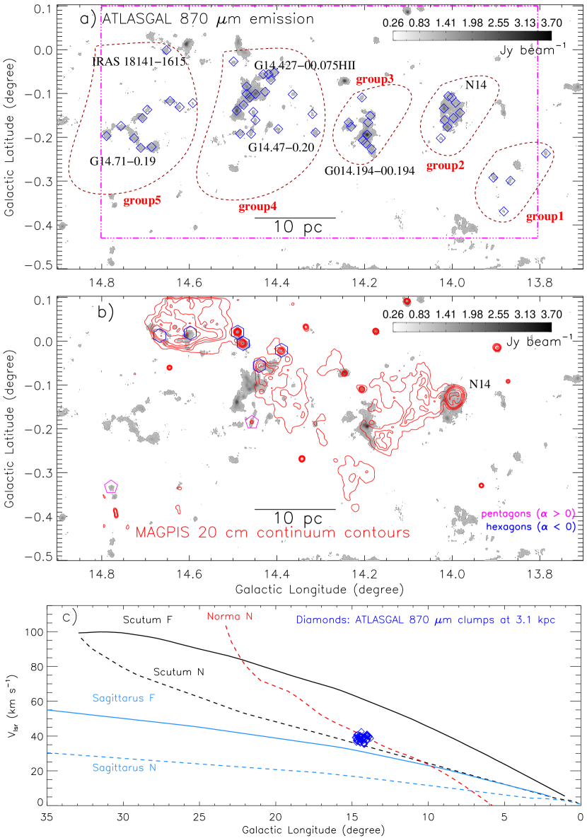
Figure 1.— a) The panel displays the ATLASGAL contour map at 870 $\mu$m (area $\sim$1$\arcdeg$.2 $\times$ 0$\arcdeg$.6 ($\sim$65 pc $\times$ 32.5 pc at a distance of 3.1 kpc); central coordinates: $l$ = 14$\arcdeg$.3; $b$ = $-$0$\arcdeg$.2) overlaid with the ATLASGAL dust continuum clumps at 870 $\mu$m (from Urquhart et al., 2018) (see diamonds). The ATLASGAL contours are shown with the levels of 3.9 Jy beam^-1 $\times$ (0.067, 0.08, 0.1, 0.15, 0.2, 0.25, 0.3, 0.4, 0.5, 0.6, 0.7, 0.8, 0.9, and 0.95). All the ATLASGAL clumps are located at a distance of $\sim$3.1 kpc. The broken box (in magenta) refers to the area shown using the MAGPIS 20 cm continuum data in Figure 1b. Some known regions (e.g., bubble N14, G014.194-00.194, G14.427-00.075HII, G14.47-0.20, IRAS 18141-1615, and G14.71-0.19) are also labeled in the figure. At least five groups of ATLASGAL clumps are indicated in the figure (see broken curves). b) Overlay of the MAGPIS 20 cm continuum contours (in red; resolution $\sim$6^′′) on the ATLASGAL contour map at 870 $\mu$m. The ATLASGAL map is the same as in Figure 1a. The MAGPIS contours are shown with the levels of 2.2, 2.8, 3.3, 4.0, 5.5, and 8.0 mJy beam^-1. The MAGPIS map is smoothed using a Gaussian function with radius of four pixels. Hexagon and Pentagon symbols represent the radio continuum sources from the THOR survey (l $>$ 14$\arcdeg$.3; Bihr et al., 2016; Wang et al., 2018). Pentagon symbols show the sources with spectral index ($\alpha$) $>$ 0, while the sources with $\alpha$ $<$ 0 are marked by hexagon symbols. c) The panel displays the Sagittarius, Scutum, and Norma arms toward l = 0$\arcdeg$.0 – 35$\arcdeg$.0 (from Reid et al., 2016) in longitude-velocity plot. The near and far sides of the arms are presented by broken and solid curves, respectively. The $V_{\mathrm{lsr}}$ of each ATLASGAL clump against its longitude is also marked in the plot. In panels a) and b), the scale bar referring to 10 pc (at a distance of 3.1 kpc) is drawn.

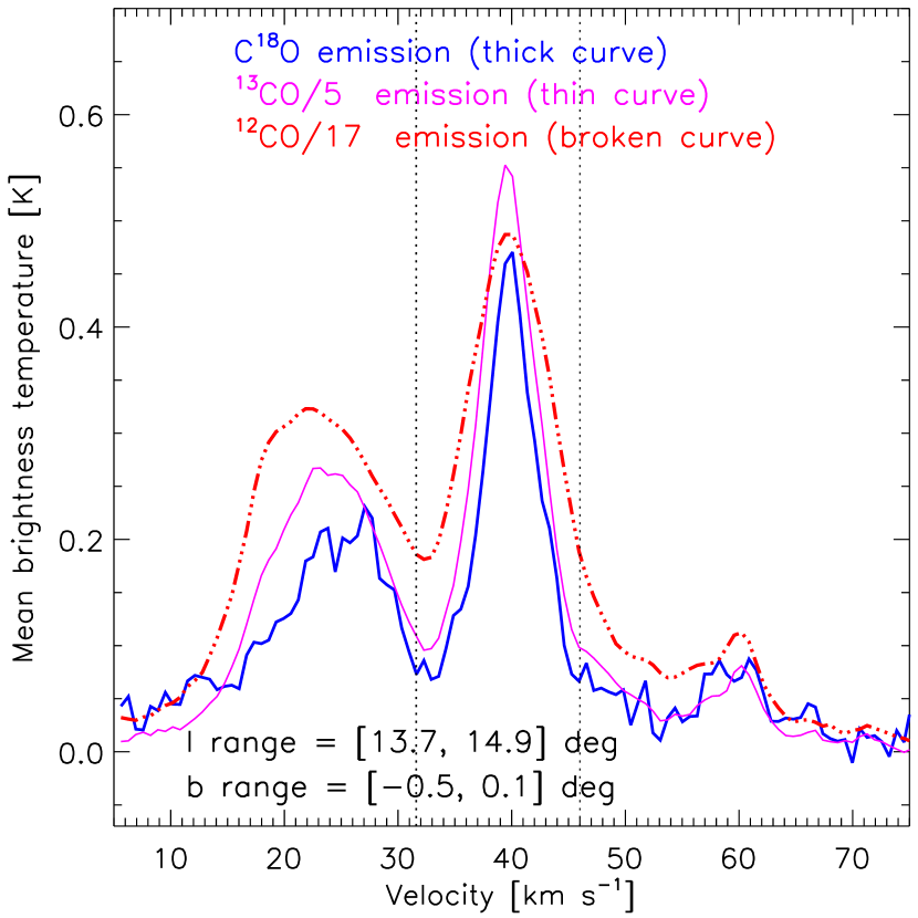
Figure 2.— The panel shows the FUGIN ¹²CO profile (broken red curve), ¹³CO spectrum (thin magenta curve), and C¹⁸O profile (thick blue curve). The profiles are produced by averaging the target area shown in Figure 1a. Ranges of the longitude and latitude of the target area are also labeled in the figure. The ¹²CO and ¹³CO spectra have been divided by a factor of 5 and 17, respectively.

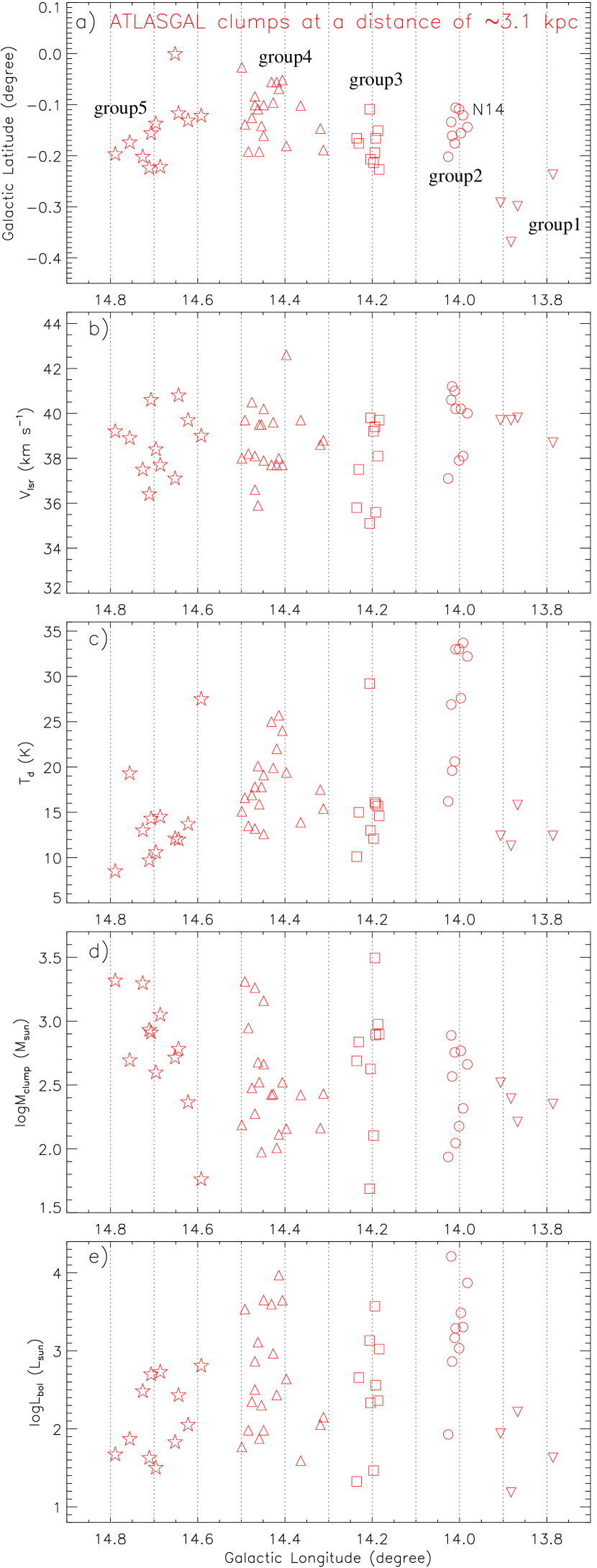
Figure 3.— a) Spatial distribution of 53 ATLASGAL dust continuum clumps at 870 $\mu$m toward the selected site. The ATLASGAL dust continuum clumps at 870 $\mu$m (from Urquhart et al., 2018) are highlighted by different symbols (i.e., up down triangles, circles, squares, triangles, and stars), which are used to show five groups of clumps (see Table 2). These groups are labeled as group1 (up down triangles), group2 (circles), group3 (squares), group4 (triangles), and group5 (stars). b-c-d-e) Distribution of the $V_{\mathrm{lsr}}$, dust temperature, mass, and bolometric luminosity of clumps against the Galactic longitude.

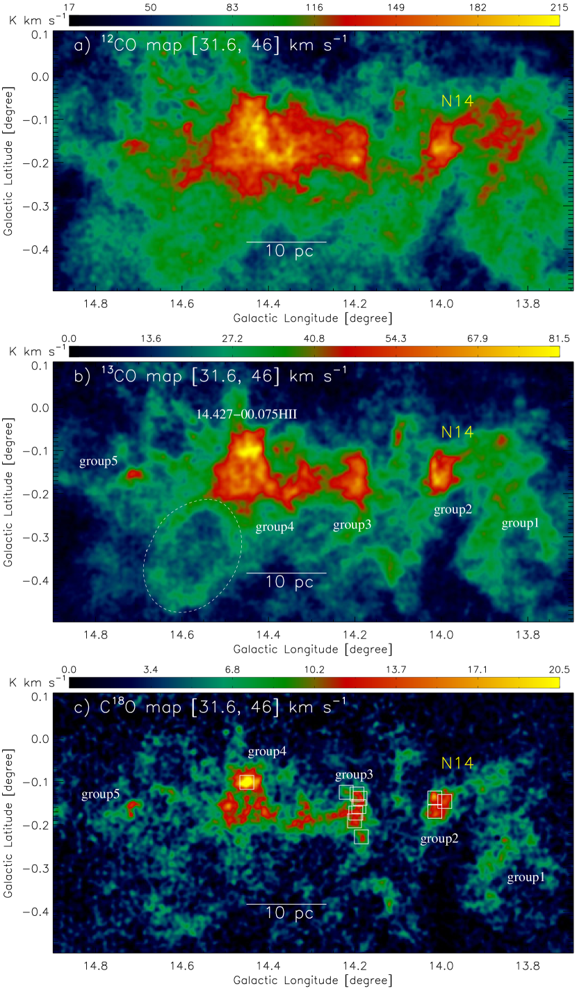
Figure 4.— a) FUGIN ¹²CO(J =1$-$0) map of intensity (moment-0) in the direction of the selected area around l = 13$\arcdeg$.7 – 14$\arcdeg$.9 and b = $-$0$\arcdeg$.5 – +0$\arcdeg$.1. b) FUGIN ¹³CO(J =1$-$0) map of intensity (moment-0). A shell-like feature is also highlighted in the panel (see a broken ellipse in white). c) FUGIN C¹⁸O(J =1$-$0) map of intensity (moment-0). Some selected molecular clumps are shown by squares. In each moment-0 map, the molecular emission is integrated from 31.6 to 46 km s^-1.

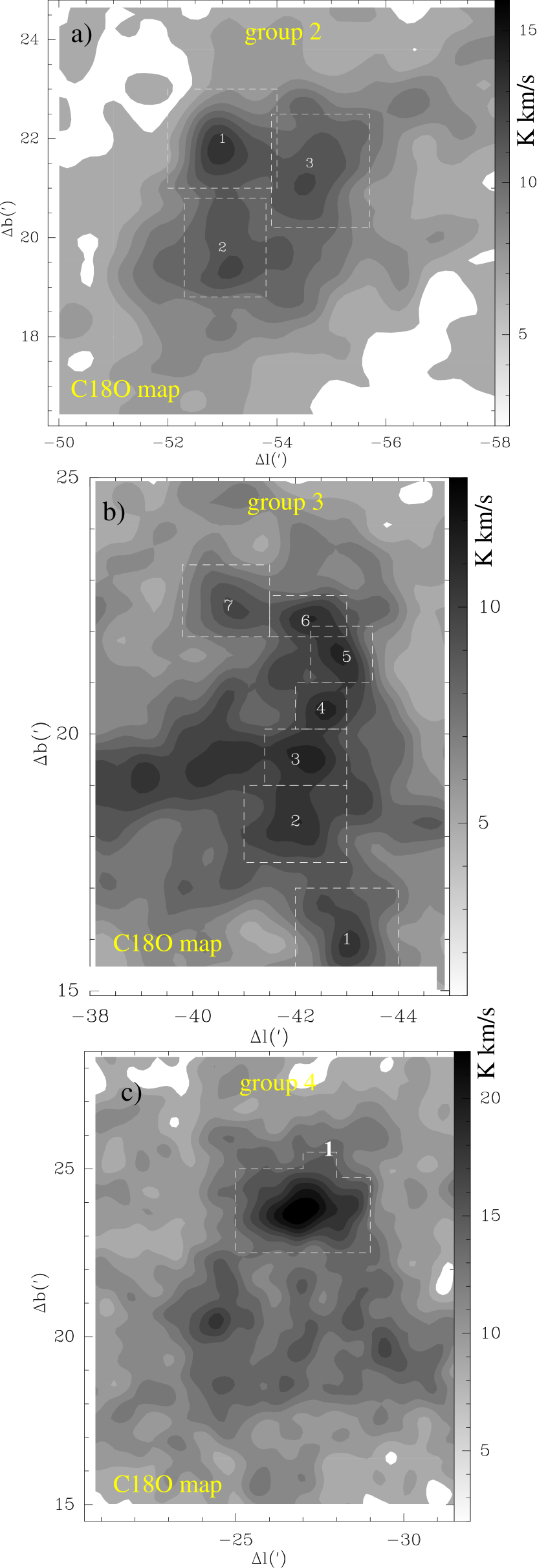
Figure 5.— Selected molecular clumps in the direction of group2, group3, and group4 using the FUGIN C¹⁸O(J =1$-$0) map (see Figure 4c and also Table 3). In each panel, the axes are offsets (in arcmin) with respect to the central position (i.e., l = 14$\arcdeg$.901; b = $-$0$\arcdeg$.499).

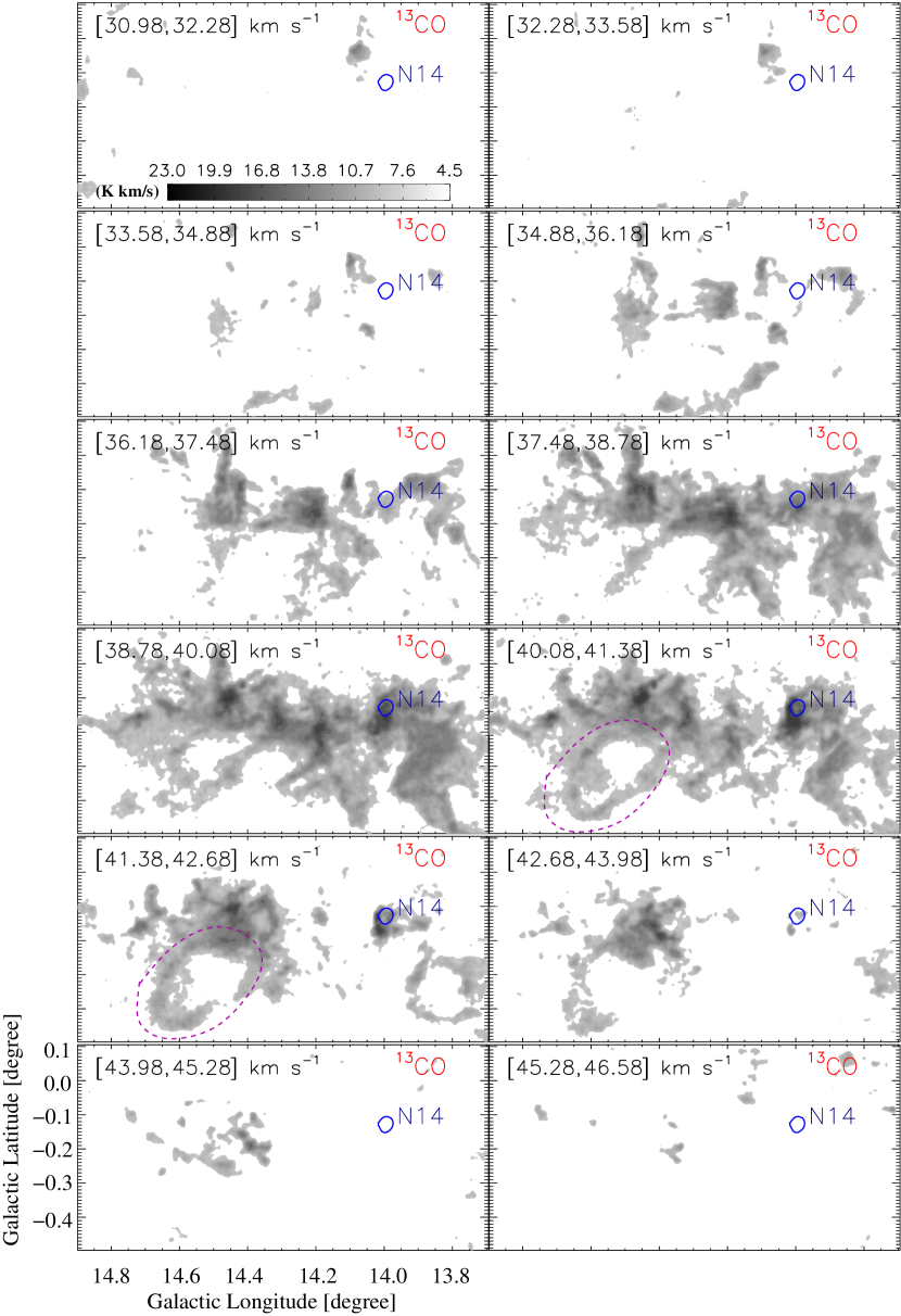
Figure 6.— The integrated velocity channel maps of ¹³CO(J =1$-$0) (at velocity intervals of 1.3 km s^-1). The bubble N14 is indicated by the MAGPIS 20 cm continuum contour (in blue) with a level of 3.7 mJy beam^-1. The ¹³CO contours are shown with the levels of 4.5, 5, 6, 7, 8, 9, 10, 11, 13, 15, 18, 21, and 23 K km s^-1. A shell-like feature is also highlighted in two panels (see a broken ellipse in magenta). The gray-scale bar in the first left panel is applicable to all the other maps.

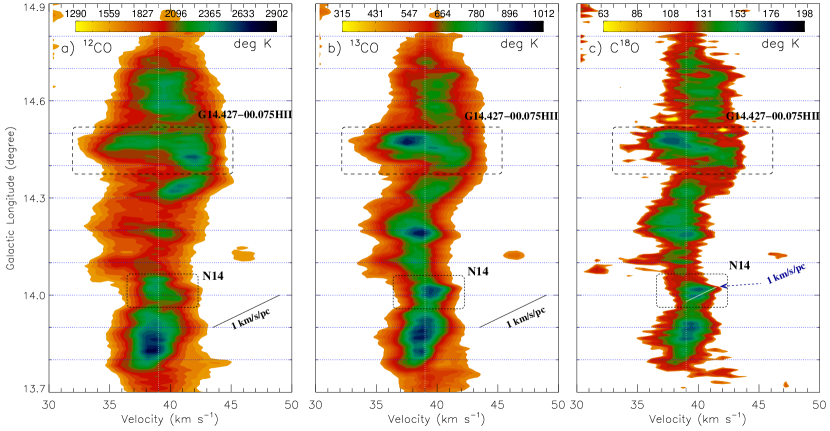
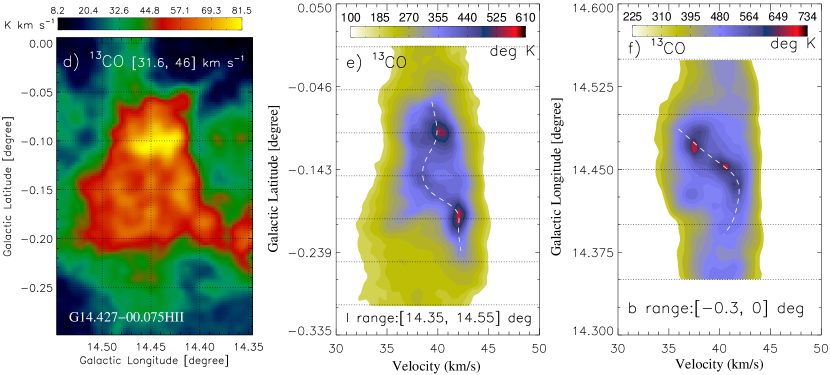
Figure 7.— Longitude-velocity maps of a) ¹²CO, b) ¹³CO and c) C¹⁸O. d) FUGIN ¹³CO integrated intensity map toward G14.427-00.075HII. e) Latitude-velocity map of ¹³CO in the direction of G14.427-00.075HII. The molecular emission is integrated over the longitude range, which is highlighted in the panel. f) Longitude-velocity map of ¹³CO toward G14.427-00.075HII. The molecular emission is integrated over the latitude range, which is labeled in the panel. In panels a), b) and c), the molecular emission is integrated over the latitude range from $-$0$\arcdeg$.5 to 0$\arcdeg$.1, and a scale bar corresponding to 1 km s^-1 pc^-1. In panels a), b) and c), the observed velocity structures toward the bubble N14 and G14.427-00.075HII are highlighted by a dotted box and a dashed box, respectively. A scale bar corresponding to 1 km s^-1 and 1 pc in the horizontal and vertical axes, respectively, is shown in panels a) and b), while a slope of 1 pc per km s^-1 is in panel c).

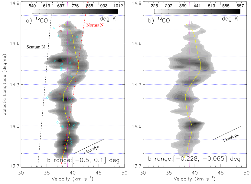
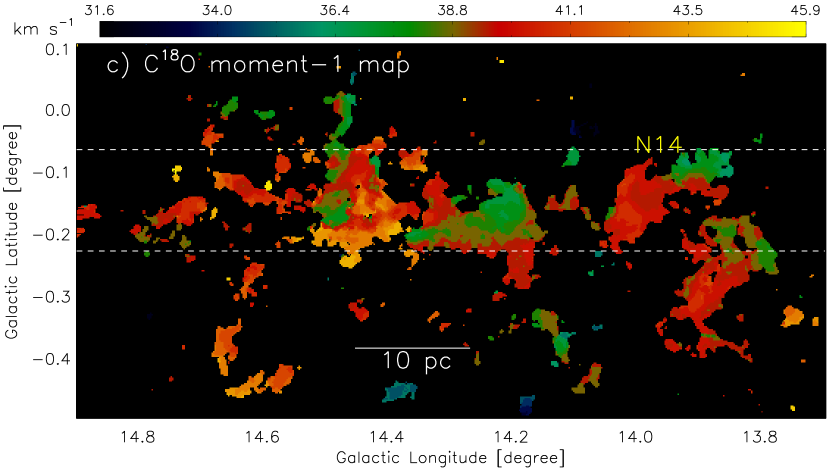
Figure 8.— a) Longitude-velocity map of ¹³CO (see also Figure 7b). The ¹³CO emission is integrated over the latitude from $-$0$\arcdeg$.5 to 0$\arcdeg$.1, and is shown between 540 and 1012 deg K. The panel also shows the Scutum and Norma arms (from Reid et al., 2016). The near side of the arms is presented by broken curves. The $V_{\mathrm{lsr}}$ of each ATLASGAL clump against its longitude is also displayed in the plot (see diamonds and also Figure 1a). Urquhart et al. (2018) reported the NH₃ line-width for some ATLASGAL clumps, which are highlighted by red diamonds in the figure (see also Table 2). b) Longitude-velocity map of ¹³CO. The ¹³CO emission is integrated over the latitude from $-$0$\arcdeg$.228 to $-$0$\arcdeg$.065. In panels a) and b), an arbitrarily chosen solid curve (in yellow) shows an oscillatory-like velocity pattern along the longitude, and a scale bar corresponding to 1 km s^-1 pc^-1 is also shown. c) Intensity-weighted mean velocity map (or the first moment map) of C¹⁸O. The color bar indicates the mean velocity (in km s^-1). Broken lines are shown at b = $-$0$\arcdeg$.228 and $-$0$\arcdeg$.065.

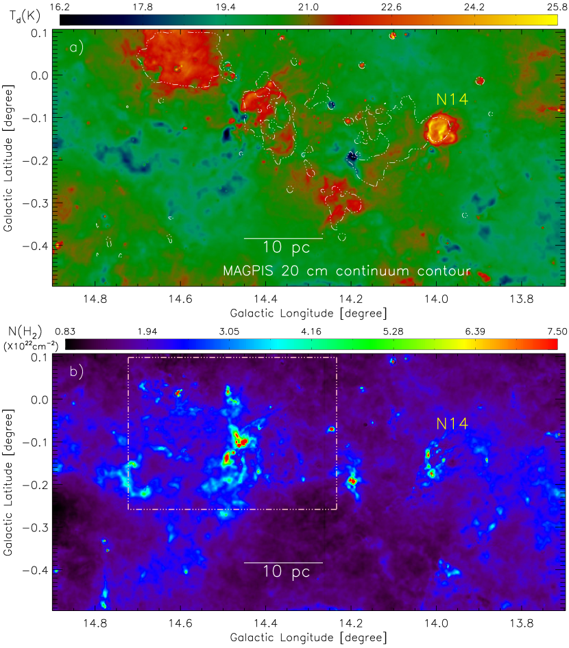
Figure 9.— a) Herschel temperature map of the selected area toward l = 13$\arcdeg$.7 – 14$\arcdeg$.9 and b = $-$0$\arcdeg$.5 – +0$\arcdeg$.1. The MAGPIS contour with a level of 2.2 mJy beam^-1 is also shown in the figure. b) Herschel column density ($N(\mathrm{H}_{2})$) map of the selected area in this paper. The dotted-dashed box encompasses the area shown in Figures 10a, 10b, and 10c.

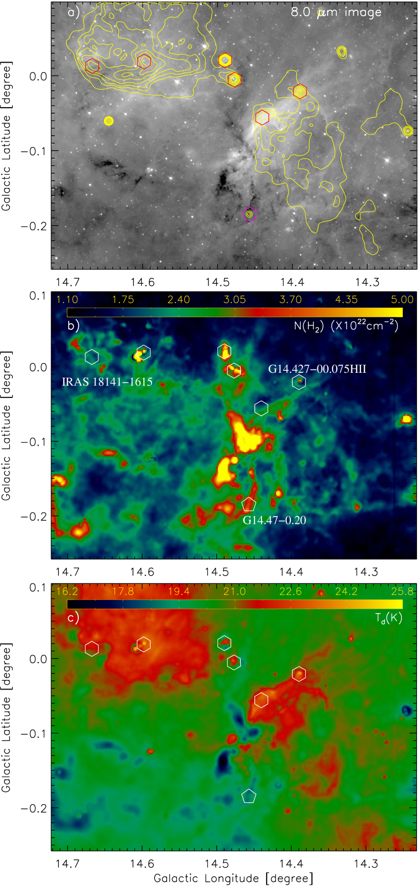
Figure 10.— A zoomed-in view of the area highlighted by a broken box in Figure 9b. a) Overlay of the MAGPIS contours and the THOR radio sources on the Spitzer 8.0 $\mu$m image. The MAGPIS contours are shown with the levels of 2.2, 2.8, 3.3, 4.0, 5.0, 6.0, and 6.7 mJy beam^-1. b) Overlay of the THOR radio sources on the Herschel column density map. c) Overlay of the THOR radio sources on the Herschel temperature map. In each panel, hexagon and pentagon symbols are the same as in Figure 1b.

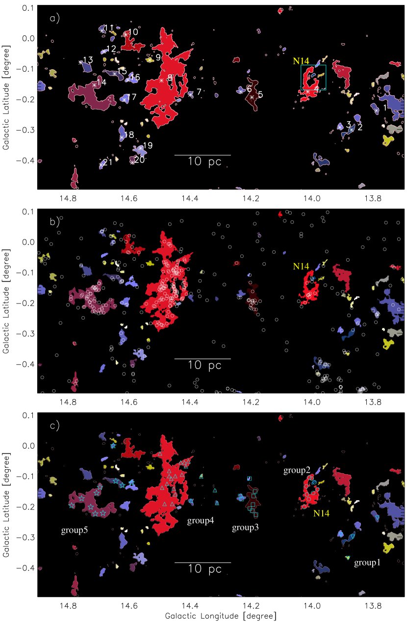
Figure 11.— a) The boundaries of several extended regions are shown in the Herschel column density map using the $N(\mathrm{H}_{2})$ contour level of 2.4 $\times$ 10²² cm^-2. Each selected extended region is highlighted by an asterisk along with its corresponding clump ID (see Table 4). The cyan box area is zoomed-in Figures 12a, 12b, 12c, and 12d. b) The positions of the identified Class I YSOs are shown toward the extended regions traced in the Herschel column density map. In this paper, the Class I YSOs, highlighted by open circles, are selected using the Spitzer color-color plot ([4.5]$-$[5.8] vs [3.6]$-$[4.5]; see text for more details). c) The positions of the ATLASGAL clumps at 870 $\mu$m are displayed toward the extended regions traced in Figure 11a. Different symbols are the same as in Figure 3a.

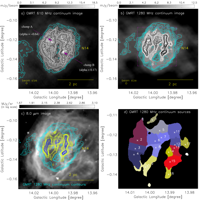
Figure 12.— a) A zoomed-in view of the bubble N14 using the GMRT 610 MHz continuum map (resolution $\sim$5^′′.56 $\times$ 5^′′.22). Cyan contours are 4 and 4.8 mJy beam^-1. White contours are 6.2, 8.0, and 9.5 mJy beam^-1. Black contours are 11, 12.5, 14, and 16 mJy beam^-1. b) A zoomed-in view of the bubble N14 using the GMRT 1280 MHz continuum map (resolution $\sim$6^′′). Cyan contours are 4.05, 4.5, 5.0, 5.5, and 6.0 mJy beam^-1. White contours are 7.6, 8.15, and 8.7 mJy beam^-1. Black contours are 9.25, 9.8, 10.35, 10.9, 11.45, 12.0, and 12.55 mJy beam^-1. The broken box (in magenta) encompasses the area shown in Figure 12d. c) Overlay of the GMRT 1280 MHz continuum contours on the Spitzer 8.0 $\mu$m image. Cyan contours are 4.05, 4.5, 5.0, 5.5, and 6.0 mJy beam^-1. Yellow contours are 7.6, 8.15, 8.7, 9.25, and 9.8 mJy beam^-1. Blue contours are 10.35, 10.9, 11.45, 12.0, and 12.55 mJy beam^-1. d) The panel shows the boundaries of several radio continuum sources at 1280 MHz, which are identified using the radio continuum contours at 1280 MHz (see Figure 12b). Each ionized clump is highlighted by an asterisk along with its corresponding clump ID. In panel a), two radio clumps “A” and “B” are identified using the GMRT radio continuum maps at 610 MHz and 1280 MHz.

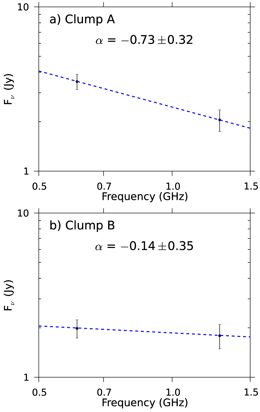
Figure 13.— a) Radio spectral index plot of the radio clump “A”, which is indicated in Figure 12a. b) Radio spectral index plot of the radio clump “B” (see Figure 12a). In each panel, filled circles (in black) are the flux densities at 610 and 1280 MHz.

Table 2Summary of the properties of 53 ATLASGAL dust clumps at 870 $\mu$m. These clumps are situated at a distance of $\sim$3.1 kpc. In the table, we have provided ID, Galactic coordinates (l, b), 870 $\mu$m integrated flux density ($S_{870}$), radial velocity ($V_{\mathrm{lsr}}$), clump effective radius ($R_{\mathrm{c}}$), dust temperature ($T_{\mathrm{d}}$), bolometric luminosity ($L_{\rm bol}$), clump mass ($M_{\mathrm{clump}}$), H₂ column density ($N(\mathrm{H}_{2})$), average volume density ($n_{\mathrm{H}_{2}}$), and virial mass ($M_{\mathrm{vir}}$). Using different symbols, five groups are indicated in Figure 3a. These groups are group1 (c1–c4; up down triangles), group2 (c5–c13; circles), group3 (c14–c22; squares), group4 (c23–c42; triangles), and group5 (c43–c53; stars). The clumps highlighted with dagger have the NH₃ line-width, and have the ratio $M_{\mathrm{clump}}$/$M_{\mathrm{vir}}$ $>$ 1 (see Urquhart et al., 2018, for more details).

ID	l	b	$S_{870}$	$V_{\mathrm{lsr}}$	Rc	$T_{\mathrm{d}}$	$L_{\rm bol}$	$M_{\mathrm{clump}}$	$N(\mathrm{H}_{2})$	$n_{\mathrm{H}_{2}}$	$M_{\mathrm{vir}}$	Association
	(degree)	(degree)	(Jy)	(km s-1)	(pc)	(K)	(102 $L_{\odot}$)	($M_{\odot}$)	(1022 cm-2)	(103 cm-3)	($M_{\odot}$)
c1	13.786	-0.237	1.96	38.7	0.15	12.4	0.4	224.4	2.9	229.8	–	group1
c2	13.867	-0.299	2.15	39.8	0.15	15.8	1.6	162.6	1.7	166.5	–	group1
c3	13.882	-0.369	1.82	39.7	0.15	11.3	0.2	247.7	2.3	253.8	–	group1
c4	13.906	-0.292	2.88	39.7	0.34	12.4	0.9	329.6	2.6	29.0	–	group1
c5	13.982	-0.144	16.60	40.0	0.48	32.2	74.3	459.2	1.8	14.4	–	group2
c6	13.992	-0.121	7.94	38.1	0.15	33.7	20.1	207.5	0.9	212.5	–	group2
c7	13.997	-0.156	17.33	40.2	0.44	27.6	30.6	586.1	1.4	23.8	–	group2
c8	14.001	-0.109	5.60	37.9	0.15	33.0	10.8	150.3	0.7	154.0	–	group2
c9	14.009	-0.106	4.13	40.2	0.15	33.0	19.5	110.9	0.7	113.6	–	group2
c10$\dagger$	14.011	-0.176	11.23	41.0	0.44	20.6	14.6	570.2	4.1	23.1	337	group2
c11	14.017	-0.161	6.76	41.2	0.30	19.6	7.3	369.0	2.4	47.2	–	group2
c12	14.019	-0.134	22.12	40.6	0.87	26.9	162.2	774.5	3.3	4.1	–	group2
c13	14.026	-0.202	1.18	37.1	0.15	16.2	0.8	86.5	1.2	88.6	–	group2
c14	14.184	-0.227	9.23	39.7	0.61	14.6	10.5	790.7	3.6	12.0	–	group3
c15	14.187	-0.151	12.47	38.1	0.46	15.7	2.3	948.4	2.1	33.7	–	group3
c16	14.192	-0.166	10.48	35.6	0.40	15.9	3.6	779.8	2.0	42.1	–	group3
c17$\dagger$	14.194	-0.194	42.86	39.4	1.12	16.1	37.2	3126.1	13.7	7.7	1694	group3
c18	14.197	-0.214	1.07	39.2	0.15	12.1	0.3	127.1	5.2	130.1	–	group3
c19	14.204	-0.207	4.04	39.8	0.15	13.0	2.2	422.7	5.0	432.9	–	group3
c20	14.206	-0.109	1.57	35.1	0.15	29.2	13.6	48.8	0.7	49.9	–	group3
c21$\dagger$	14.231	-0.176	8.40	37.5	0.61	15.0	4.5	687.1	3.1	10.5	333	group3
c22	14.236	-0.166	2.90	35.8	0.21	10.1	0.2	488.7	4.2	182.4	–	group3
c23$\dagger$	14.312	-0.189	3.45	38.8	0.27	15.4	1.4	270.4	2.4	47.5	184	group4
c24	14.319	-0.147	2.27	38.6	0.15	17.5	1.1	145.2	1.3	148.7	–	group4
c25	14.364	-0.102	2.84	39.7	0.15	13.9	0.4	264.2	1.8	270.7	–	group4
c26	14.397	-0.181	2.63	42.6	0.21	19.4	4.4	143.9	1.1	53.7	–	group4
c27	14.406	-0.052	8.22	37.7	0.82	24.0	44.4	331.9	1.2	2.1	–	group4
c28	14.414	-0.069	3.53	38.0	0.58	25.7	93.1	129.7	1.2	2.3	–	group4
c29	14.419	-0.056	2.23	37.7	0.15	22.0	2.7	101.6	1.3	104.1	–	group4
c30	14.427	-0.096	5.11	39.6	0.37	19.9	9.2	269.2	1.4	18.4	–	group4
c31	14.431	-0.056	6.96	37.7	0.31	25.0	39.5	265.5	0.8	30.8	–	group4
c32$\dagger$	14.449	-0.101	25.78	40.2	0.76	19.1	44.8	1445.4	6.0	11.4	1247	group4
c33	14.449	-0.161	4.17	37.9	0.15	12.6	1.0	460.3	2.7	471.4	–	group4
c34	14.454	-0.142	1.51	39.5	0.15	17.8	2.0	94.2	1.8	96.5	–	group4
c35	14.459	-0.192	4.47	39.5	0.15	15.9	0.7	332.7	1.7	340.7	–	group4
c36	14.462	-0.109	9.18	35.9	0.40	20.1	12.9	476.4	4.9	25.7	–	group4
c37$\dagger$	14.469	-0.084	17.96	38.1	0.72	13.2	7.3	1828.1	7.2	16.9	662	group4
c38	14.469	-0.101	3.02	36.6	0.15	17.8	3.2	188.4	4.2	192.9	–	group4
c39	14.476	-0.126	4.44	40.5	0.28	16.9	2.2	299.9	4.6	47.2	–	group4
c40	14.484	-0.192	9.05	38.2	0.39	13.5	1.0	885.1	2.4	51.6	–	group4
c41$\dagger$	14.492	-0.139	29.46	39.7	1.12	16.6	34.2	2046.4	9.0	5.0	1837	group4
c42	14.499	-0.027	1.90	38.0	0.15	15.1	0.6	153.8	1.6	157.6	–	group4
c43	14.592	-0.122	1.72	39.0	0.15	27.5	6.4	57.7	0.6	59.1	–	group5
c44	14.622	-0.131	2.43	39.7	0.30	13.7	1.1	231.7	2.1	29.7	–	group5
c45	14.644	-0.117	5.02	40.8	0.46	12.0	2.7	606.7	4.1	21.5	–	group5
c46	14.652	-0.001	4.36	37.1	0.30	12.1	0.7	518.8	3.6	66.4	–	group5
c47$\dagger$	14.686	-0.222	12.92	37.7	0.78	14.5	5.4	1119.4	3.6	8.2	495	group5
c48	14.696	-0.137	2.59	38.4	0.25	10.6	0.3	396.3	3.1	87.7	–	group5
c49$\dagger$	14.707	-0.156	9.20	40.6	0.66	14.3	5.0	814.7	3.7	9.8	638	group5
c50	14.711	-0.224	4.66	36.4	0.42	9.7	0.4	853.1	4.9	39.8	–	group5
c51$\dagger$	14.726	-0.202	18.98	37.5	0.70	13.0	3.0	1981.5	3.8	20.0	156	group5
c52	14.756	-0.174	8.96	38.9	0.24	19.3	0.7	494.3	1.1	123.6	–	group5
c53	14.789	-0.197	8.53	39.2	0.49	8.5	0.5	2079.7	6.7	61.1	–	group5

Table 3Physical parameters of selected molecular clumps in the direction of group2, group3, and group4 using the C¹⁸O line data, which are indicated in Figure 5. Column 1 shows the IDs assigned to the molecular clump(s). Table also contains central positions (l, b), C¹⁸O clump diameter (D_c), mass derived from C¹⁸O ($M_{\mathrm{mc}}$), Full Width Half Maximum (C¹⁸O $\Delta V$), M_vir, and mean number density ($\bar{n}$) calculated from $M_{\mathrm{mc}}$ and D_c. Note that the C¹⁸O spectra toward the clumps g3clm5 and g3clm6 contain two closely located velocity components, which do not allow to determine their line widths. Hence the values of M_vir are not computed for the clumps g3clm5 and g3clm6.

ID	l	b	Dc	$M_{\mathrm{mc}}$	$\Delta V$	Mvir	$\bar{n}$	Association
	(degree)	(degree)	(pc)	($M_{\odot}$)	(km s-1)	($M_{\odot}$)	(104 cm-3)
g2clm1	14.015	-0.138	2.22	4265	3.77	3360	1.30	group2
g2clm2	14.015	-0.169	1.43	3930	3.03	1380	4.46	group2
g2clm3	13.992	-0.146	2.50	4930	3.02	2390	1.06	group2
g3clm1	14.185	-0.228	1.39	3575	2.93	1250	4.46	group3
g3clm2	14.201	-0.191	1.30	3530	3.85	2040	5.27	group3
g3clm3	14.198	-0.173	1.43	2200	3.57	1910	2.52	group3
g3clm4	14.191	-0.158	0.60	1210	3.40	733	18.20	group3
g3clm5	14.188	-0.139	1.87	1630	–	–	0.84	group3
g3clm6	14.195	-0.129	1.11	1470	–	–	3.59	group3
g3clm7	14.220	-0.125	1.27	1890	4.01	2140	3.07	group3
g4clm1	14.450	-0.102	1.99	16230	5.43	6130	6.92	group4

Table 4Physical parameters of extended regions identified in the Herschel column density map, which are highlighted in Figure 11a. Column 1 lists the IDs given to the extended region. Table also contains positions, deconvolved effective radius ($R_{\mathrm{c}}$), and clump mass ($M_{\mathrm{clump}}$).

ID	l	b	$R_{\mathrm{c}}$	$M_{\mathrm{clump}}$	Association
	[degree]	[degree]	(pc)	($M_{\odot}$)
h1	13.789	-0.238	0.70	880	group1
h2	13.870	-0.301	0.74	1040	group1
h3	13.910	-0.293	0.53	525	group1
h4	14.014	-0.176	1.68	6175	group2
h5	14.197	-0.195	1.51	5400	group3
h6	14.234	-0.176	0.60	665	group3
h7	14.399	-0.186	0.47	420	group4
h8	14.494	-0.140	4.44	42975	group4
h9	14.532	-0.073	0.49	425	group4
h10	14.610	0.010	1.40	4045	group5
h11	14.689	0.024	0.56	635	group5
h12	14.682	-0.045	0.43	335	group5
h13	14.759	-0.081	0.86	1405	group5
h14	14.714	-0.155	2.55	13135	group5
h15	14.647	-0.118	0.92	1670	group5
h16	14.604	-0.138	0.77	1085	group5
h17	14.615	-0.203	0.76	1055	group5
h18	14.624	-0.326	0.86	1395	group4
h19	14.562	-0.361	0.90	1415	group4
h20	14.589	-0.408	0.60	710	group4
h21	14.692	-0.416	0.52	490	group4

Table 5Physical parameters of 17 radio clumps traced in the GMRT 1280 MHz continuum map, which are labeled in Figure 12d. Table contains ID, Galactic coordinates (l, b), deconvolved effective radius of the H ii region ($R_{\mathrm{HII}}$), total flux ($S{{}_{\nu}}$), Lyman continuum photons ($\log{N_{\mathrm{uv}}}$), dynamical age ($t_{\mathrm{dyn}}$), and radio spectral type.

ID	l	b	$R_{\mathrm{HII}}$	$S{{}_{\nu}}$	$\log{N_{\mathrm{uv}}}$	$t_{\mathrm{dyn}}$	Spectral Type
	(degree)	(degree)	(pc)	(mJy)	(s-1)	($\times$ 103 yr)	(dwarf main-sequence (V))
g1	13.999	-0.112	0.10	26	46.29	1.1	B0.5-B1
g2	14.006	-0.123	0.27	238	47.25	9.8	B0-B0.5
g3	14.007	-0.127	0.17	98	46.87	4.0	B0-B0.5
g4	14.008	-0.130	0.21	142	47.03	5.8	B0-B0.5
g5	13.995	-0.118	0.20	121	46.96	6.3	B0-B0.5
g6	13.997	-0.123	0.17	97	46.86	4.2	B0-B0.5
g7	13.994	-0.121	0.15	74	46.75	3.0	B0-B0.5
g8	13.997	-0.127	0.16	77	46.76	3.7	B0-B0.5
g9	14.000	-0.135	0.13	47	46.55	2.6	B0-B0.5
g10	14.002	-0.136	0.14	58	46.64	3.3	B0-B0.5
g11	13.987	-0.119	0.20	133	47.00	5.8	B0-B0.5
g12	13.987	-0.125	0.14	68	46.71	2.2	B0-B0.5
g13	13.988	-0.127	0.14	62	46.66	2.3	B0-B0.5
g14	13.990	-0.129	0.11	35	46.42	1.5	B0.5-B1
g15	13.990	-0.134	0.20	127	46.98	5.1	B0-B0.5
g16	13.990	-0.140	0.11	34	46.41	1.7	B0.5-B1
g17	13.982	-0.125	0.13	46	46.54	2.3	B0-B0.5

References

- Arce et al. (2011) Arce, H. G., Borkin, M. A., Goodman, A. A., Pineda, J. E.,& Beaumont, C. N. 2011, ApJ, 742, 105
- Ballesteros-Paredes et al. (1999) Ballesteros-Paredes, J., Hartmann, L., & Vázquez-Semadeni, E. 1999, ApJ, 527, 285
- Barnes et al. (2019) Barnes, A. T., Longmore, S. N., Avison, A., et al. 2019, arXiv:1903.06158
- Baug et al. (2019) Baug, T., de Grijs Richard, Dewangan, L. K., et al. 2019, ApJ, 885, 68
- Baug et al. (2015) Baug, T., Ojha, D. K., Dewangan, L. K., et al. 2015, MNRAS, 454, 4335
- Beaumont and Williams (2010) Beaumont, C. N., & Williams, J. P. 2010, ApJ, 709, 791
- Benjamin et al. (2003) Benjamin, R. A.,Churchwell, E., Babler, B. L., et al. 2003, PASP, 115, 953
- Beuther et al. (2015) Beuther, H., Henning, T., Linz, H., et al. 2015, A&A, 581, A119
- Beuther et al. (2016) Beuther, H., Bihr, S. , Rugel, M., et al. 2016, A&A, 595, 32
- Bihr et al. (2016) Bihr, S. , Johnston, K. G., Beuther, H., et al. 2016, A&A, 588, 97
- Bisbas et al. (2015) Bisbas, T. G., Haworth, T. J., Williams, R. J. R., et al. 2015, MNRAS, 453, 1324
- Burkert & Hartmann (2004) Burkert, A., & Hartmann, L. 2004, ApJ, 616, 288
- Carey et al. (2005) Carey, S. J., Noriega-Crespo, A., Price, S. D., et al. 2005, BAAS, 37, 1252
- Churchwell et al. (2006) Churchwell, E., Povich, M. S., Allen, D., et al. 2006, ApJ, 649, 759
- Csengeri et al. (2017) Csengeri, T., Bontemps, S., Wyrowski, F., et al. 2017, A&A, 600, L10
- Dale et al. (2007) Dale, J. E., Clark, P. C., & Bonnell, I. A. 2007, MNRAS, 377, 535
- De Becker (2018) De Becker, M. 2018, A&A, 620, 144
- Deharveng et al. (2005) Deharveng, L., Zavagno, A., & Caplan, J. 2005, A&A, 433, 565
- Dewangan and Ojha (2013) Dewangan, L. K., & Ojha, D. K. 2013, MNRAS, 429, 1386
- Dewangan et al. (2015) Dewangan, L. K., Luna, A., Ojha, D. K., et al. 2015, ApJ, 811, 79
- Dewangan et al. (2016a) Dewangan, L. K., Ojha, D. K., Luna, A., et al. 2016a, ApJ, 819, 66
- Dewangan et al. (2016b) Dewangan, L. K., Baug, T., Ojha, D. K., et al. 2016b, ApJ, 826, 27
- Dewangan et al. (2017) Dewangan, L. K., Ojha, D. K., Zinchenko, I., Janardhan, P., & Luna, A. 2017, ApJ, 834, 22
- Dewangan et al. (2019) Dewangan, L. K., Pirogov, L. E., Ryabukhina, O. L., Ojha, D. K., & Zinchenko, I. 2019, ApJ, 877, 1
- Dyson & Williams (1980) Dyson, J. E., & Williams, D. A. 1980, Physics of the interstellar medium, New York, Halsted Press, 204 p
- Elmegreen & Lada (1977) Elmegreen, B. G., & Lada, C. J. 1977, ApJ, 214, 725
- Elmegreen (1998) Elmegreen, B. G. 1998, in ASP Conf. Ser. 148, Origins, ed. C. E. Woodward, J. M. Shull, & H. A. Thronson, Jr. (San Francisco, CA: ASP), 150
- Evans et al. (2009) Evans, N. J., II, Dunham, M. M., Jrgensen, J. K., et al. 2009, ApJS, 181, 321
- Frerking et al. (1982) Frerking, M. A., Langer, W. D., & Wilson, R. W. 1982, ApJ, 262, 590
- Friesen et al. (2016) Friesen, R. K., Bourke, T. L., Di Francesco, J., Gutermuth, R., & Myers, P. C. 2016, ApJ, 833, 204
- Galván-Madrid et al. (2009) Galván-Madrid, R., Keto, E., Zhang, Q., et al. 2009, ApJ, 706, 1036
- Getman et al. (2007) Getman, K. V., Feigelson, E. D., Garmire,G., Broos, P., & Wang, J. 2007, ApJ, 654, 316
- Habe & Ohta (1992) Habe, A., & Ohta, K. 1992, PASJ, 44, 203
- Hacar & Tafalla (2011) Hacar, A. & Tafalla, M. 2011, A&A, 533, 34
- Hacar et al. (2017) Hacar, A., Alves, J., Tafalla, M., & Goicoechea, J. R. 2017, A&A, 602, L2
- Haid et al. (2019) Haid, S., Walch, S., Seifried, D., Wünsch, R., Dinnbier, F., & Naab, T., 2019, MNRAS, 482, 4062
- Heitsch & Hartmann (2008) Heitsch, F., & Hartmann, L. 2008, ApJ, 689, 290
- Heitsch et al. (2008) Heitsch, F., Hartmann, L. W., Slyz, A. D., Devriendt, J. E.G., & Burkert, A. 2008, ApJ, 674, 316
- Heitsch et al. (2009) Heitsch, F., Ballesteros-Paredes, J., & Hartmann, L. 2009, ApJ, 704, 1735
- Hartmann et al. (2005) Hartmann, L., Megeath, S. T., Allen, L., et al. 2005, ApJ, 629, 881
- Hartmann & Burkert (2007) Hartman, L., & Burkert, A., 2007, ApJ, 654, 988.
- Hartmann et al. (2012) Hartmann, L., Ballesteros-Paredes, J., Heitsch, F. 2012, MNRAS, 420, 1457
- Helfand et al. (2006) Helfand, D. J., Becker, R. H., White, R. L., Fallon, A., & Tuttle, S. 2006, AJ, 131, 2525
- Hennebelle & Falgarone (2012) Hennebelle, P. & Falgarone, E. 2012, A&ARv, 20, 55
- Hoare et al. (2012) Hoare, M. G., Purcell, C. R., Churchwell, E. B., et al. 2012, PASP, 124, 939
- Jackson et al. (2019) Jackson, J. M., Whitaker, J. S., Rathborne, J. M., et al. 2019, ApJ, 870, 5
- Jin et al. (2016) Jin, M., Lee, J.-E., Kim, K.-T., & Evans, N. J., II 2016, ApJS, 225, 21
- Kim et al. (2018) Kim, Jeong-Gyu, Kim, Woong-Tae, & Ostriker, E. C. 2018, ApJ, 859, 68
- Kurtz (2005) Kurtz, S. 2005, in Massive Star Birth: A Crossroads of Astrophysics, eds. R. Cesaroni, M. Felli, E. Churchwell, & M. Walmsley, IAU Symp., 227, 111
- Liu et al. (2015) Liu, H. B., Galván-Madrid, R., Jiménez-Serra, I., et al. 2015, ApJ, 804, 37
- Liu et al. (2016b) Liu, T., Kim, K.-T., Yoo, H., et al. 2016, ApJ, 829, 59
- Longair (1992) Longair, M. S. 1992, High energy astrophysics. Vol.1: Particles, photons and their detection, 436
- MacLaren et al. (1988) MacLaren, I., Richardson, K. M., & Wolfendale, A. W. 1988, ApJ, 333, 821
- Mangum & Shirley (2016) Mangum, J. G. & Shirley, Y. L. 2016, PASP, 128, 9201
- Mallick et al. (2012) Mallick, K. K., Ojha, D. K., Samal, M. R., et al. 2012, ApJ, 759, 48
- Mallick et al. (2013) Mallick, K. K., Kumar, M. S. N., Ojha, D. K., et al. 2013, ApJ, 779, 113
- Marsh et al. (2015) Marsh, K. A., Whitworth, A. P., & Lomax, O. 2015, MNRAS, 454, 4282
- Marsh et al. (2017) Marsh, K. A., Whitworth, A. P., Lomax, O., et al. 2017, MNRAS, 471, 2730
- Martins et al. (2005) Martins, F., Schaerer, D., & Hillier, D. J. 2005, A&A, 436, 1049
- Matsakis et al. (1976) Matsakis, D. N., Evans, N. J., II, Sato, T., & Zuckerman, B. 1976, AJ, 81, 172
- Molinari et al. (2010a) Molinari, S., Swinyard, B., Bally, J., et al., 2010a, A&A, 518, L100
- Molinari et al. (2010b) Molinari, S., Swinyard, B., Bally, J., et al., 2010b, PASP, 122, 314
- Nandakumar et al. (2016) Nandakumar, G., Veena, V. S., Vig, S., et al. 2016, AJ, 152, 146
- Padovani et al. (2019) Padovani, M., Marcowith, A., Sánchez-Monge, Á., Meng, F., & Schilke, P. 2019, A&A, 630, A72
- Panagia (1973) Panagia, N. 1973, AJ, 78, 929
- Peretto et al. (2013) Peretto, N., Fuller, G. A., Duarte-Cabral, A., et al. 2013, A&A, 555, A112
- Purcell et al. (2013) Purcell, C. R., Hoare, M. G., Cotton, W. D., et al. 2013, ApJS, 205, 1
- Reid et al. (2016) Reid, M. J., Dame, T. M., Menten, K. M., & Brunthaler, A. 2016, ApJ, 823, 77
- Rybicki & Lightman (1979) Rybicki, G. B., and Lightman, A. P. 1979, Radiative processes in astrophysics
- Sánchez-Monge et al. (2008) Sánchez-Monge, Á., Palau, A., Estalella, R., Beltrán, M. T., & Girart, J. M. 2008, A&A, 485, 497
- Sánchez-Monge et al. (2011) Sánchez-Monge, Á., Pandian, J. D., & Kurtz, S. 2011, ApJ, 739, L9
- Schuller et al. (2009) Schuller, F., Menten, K. M., Contreras, Y., et al. 2009, A&A, 504, 415
- Sherman (2012) Sherman, R. A. 2012, ApJ, 760, 58
- Tan et al. (2014) Tan, J. C., Beltrán, M. T., Caselli, P., et al. 2014, in Protostars and Planets VI, ed. H. Beuther et al. (Tucson, AZ: Univ. Arizona Press), 149
- Urquhart et al. (2018) Urquhart, J. S., König, C., Giannetti, A., et al. 2018, MNRAS, 473, 1059
- Umemoto et al. (2017) Umemoto, T., Minamidani, T., Kuno, N., et al. 2017 PASJ, 69, 78
- Vázquez-Semadeni et al. (2007) Vázquez-Semadeni, E., Gómez, G. C., Jappsen, A. K., Ballesteros-Paredes, J., González, R. F., & Klessen, R. S. 2007, ApJ, 657, 870
- Vázquez-Semadeni et al. (2019) Vázquez-Semadeni, E., Palau, A., Ballesteros-Paredes, J., Gómez, G. C., & Zamora-Avilés, M. 2019, accepted in MNRAS, arXiv:1903.11247
- Veena et al. (2016) Veena, V. S., Vig, S., Tej, A., et al. 2016, MNRAS, 456, 2425
- Walch et al. (2015) Walch, S., Whitworth, A. P., Bisbas, T. G., Hubber, D. A., & Wünsch, R. 2015, MNRAS, 452, 2794
- Wang et al. (2018) Wang, Y., Bihr, S., Rugel, M., et al. 2018, A&A, 619, 124
- Whitworth et al. (1994) Whitworth, A. P., Bhattal, A. S., Chapman, S. J., Disney, M. J., & Turner, J. A. 1994, MNRAS, 268, 291
- Williams et al. (1994) Williams, J. P., de Geus, E. J., & Blitz, L. 1994, ApJ, 428, 693
- Wilson et al. (2005) Wilson, B. A., Dame, T. M., Masheder, M. R. W., & Thaddeus, P. 2005, A&A, 430, 523
- Wood & Churchwell (1989) Wood, D. O. S., & Churchwell, E. 1989, ApJS, 69, 831
- Yan et al. (2016) Yan, Q. Z., Xu, Y., Zhang, B., et al. 2016, AJ, 152, 117
- Yang et al. (2019) Yang, A. Y., Thompson, M. A., Tian, W. W., et al. 2019, MNRAS, 482, 2681
- Yuan et al. (2018) Yuan, J., Li, J.-Z., Wu, Y., et al. 2018, ApJ, 852, 12
- Zinnecker & Yorke (2007) Zinnecker, H., & Yorke, H. W. 2007, ARA&A, 45, 481