Deep Implicit Volume Compression

Abstract

We describe a novel approach for compressing truncated signed distance fields (TSDF) stored in 3D voxel grids, and their corresponding textures. To compress the TSDF, our method relies on a block-based neural network architecture trained end-to-end, achieving state-of-the-art rate-distortion trade-off. To prevent topological errors, we losslessly compress the signs of the TSDF, which also upper bounds the reconstruction error by the voxel size. To compress the corresponding texture, we designed a fast block-based UV parameterization, generating coherent texture maps that can be effectively compressed using existing video compression algorithms. We demonstrate the performance of our algorithms on two 4D performance capture datasets, reducing bitrate by $66\%$ for the same distortion, or alternatively reducing the distortion by $50\%$ for the same bitrate, compared to the state-of-the-art.

1 Introduction

In recent years, volumetric implicit representations have been at the heart of many 3D and 4D reconstruction approaches [27, 45, 26, 22], enabling novel applications such as real time dense surface mapping in AR devices and free-viewpoint videos. While these representations exhibit numerous advantages, transmitting high quality 4D sequences is still a challenge due to their large memory footprints. Designing efficient compression algorithms for implicit representations is therefore of prime importance to enable the deployment of novel consumer-level applications such as VR/AR telepresence [47], and to facilitate the streaming of free-viewpoint videos [8].

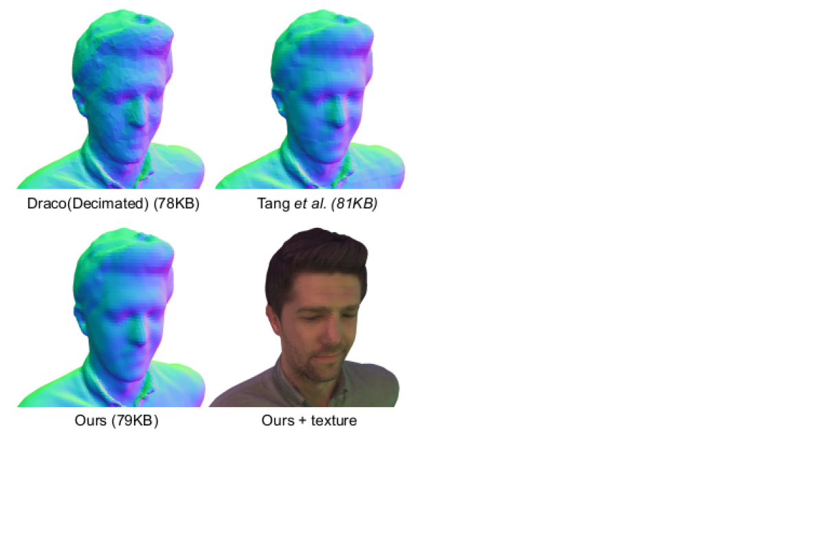
Figure 1: When targeting a low bitrate, Draco [24] requires decimation to have low-poly meshes as input, while [59] suffers from block artifacts. Our method has visibly lower distortion while maintaining similar bitrates. Raw meshes with flat shading are shown to reveal artifacts.

In contrast to compressing a mesh, it was recently shown that truncated signed distance fields (TSDF) [15] are highly suitable for efficient compression [59, 31] due to correlation in voxel values and their regular grid structure. Voxel-based SDF representations have been used with great success for 3D shape learning using encoder-decoder architectures [58, 65]. This is in part due to their grid structure that can be naturally processed with 3D convolutions, allowing the use of convolutional neural networks (CNN) that have excelled in image processing tasks. Based on these observations, we propose a novel block-based encoder-decoder neural architecture trained end-to-end, achieving bitrates that are $33\%$ of prior art [59]. We compress and transmit the TSDF signs losslessly; this does not only guarantee that the reconstruction error is upper bounded by the voxel size, but also that the reconstructed surface is homeomorphic – even when lossy TDSF compression is used. Furthermore, we propose using the conditional distribution of the signs given the encoded TSDF block to compress the signs losslessly, leading to significant gains in bitrates. This also significantly reduces artifacts in the reconstructed geometry and textures.

Recent 3D and 4D reconstruction pipelines not only reconstruct accurate geometry, but also generate high quality texture maps, e.g. $4096{\times}4096$ pixels, that need to be compressed and transmitted altogether with the geometry [26]. To complement our TSDF compression algorithm, we developed a fast parametrization method based on block-based charting, which encourages spatio-temporal coherence without tracking. Our approach allows efficient compression of textures using existing image-based techniques and removes the need of compressing and streaming UV coordinates.

To summarize, we propose a novel block-based 3D compression model with these contributions:

1. the first deep 3D compression method that can train end-to-end with entropy encoding, yielding state-of-the-art performance;

2. lossless compression of the surface topology using the conditional distribution of the TSDF signs, and thereby bounding the reconstruction error by the size of a voxel;

3. a novel block-based texture parametrization that inherently encourages temporal consistency, without tracking or the necessity of UV coordinates compression.

2 Related works

Compression of 3D/4D media (e.g., meshes, point clouds, volumes) is a fundamental problem for applications such as VR/AR, yet has received limited attention in the computer vision community. In this section, we describe two main aspects of 3D compression: geometry and texture, as well as reviewing recent trends in learnable compression.

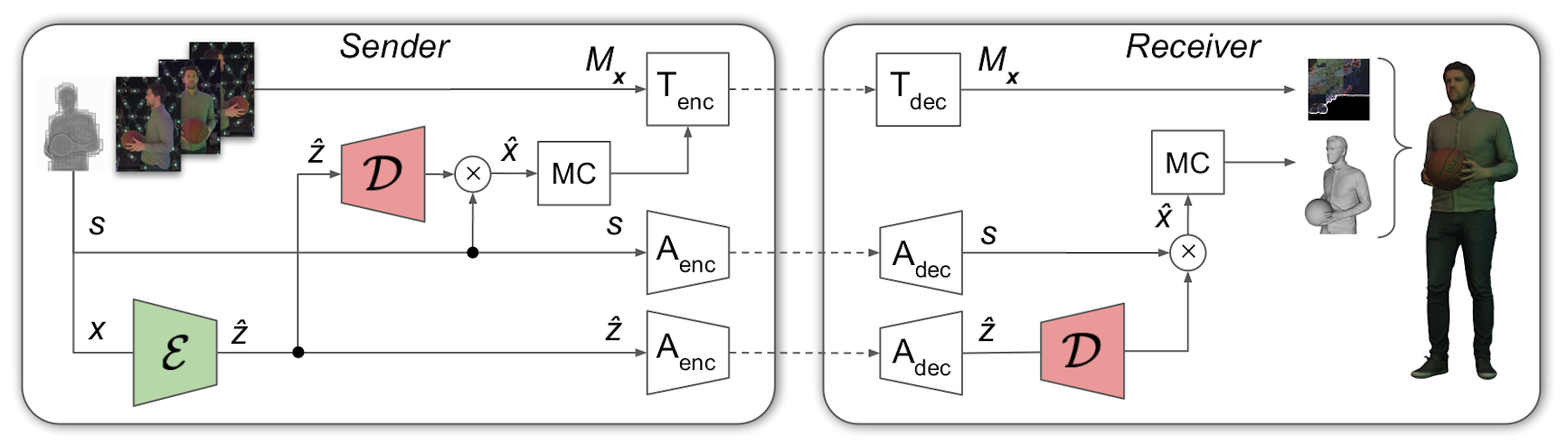
Figure 2: Compression pipeline – Given an input TSDF block $\bm{x}$ and its sign configuration $\mathbf{s}{=}\operatorname{sign}(\bm{x})$, an encoder transforms $\bm{x}$ into a quantized code $\hat{\mathbf{z}}{=}\lfloor\mathcal{E}(\bm{x})\rceil$. Then $\hat{\mathbf{z}}$ and $\mathbf{s}$ are entropy coded and transmitted to the receiver ($A_{\text{enc}}$ and $A_{\text{dec}}$ blocks) using a prior learned distribution $p_{\hat{\mathbf{z}}}(\hat{\mathbf{z}})$ and the conditional distribution $p_{\mathbf{s}|\hat{\mathbf{z}}}(\mathbf{s}|\hat{\mathbf{z}})$ as estimated by the decoder, respectively. The reconstructed block $\hat{\bm{x}}{=}\mathbf{s}\odot|\mathcal{D}(\hat{\mathbf{z}})|$ is used with marching cubes (MC in the figure) to extract the mesh, which is then used to generate the Morton packed chart $M_{x}$. $M_{x}$ is coded separately (with the $T_{\text{enc}}$ and $T_{\text{dec}}$ blocks).

Geometry compression

Geometric surface representations can either be explicit or implicit. While explicit representations are dominant in traditional computer graphics [4, 13], implicit representations have found widespread use in perception related tasks such as real-time volumetric capture [21, 27, 45, 20]. Explicit representations include meshes, point clouds, and parametric surfaces (NURBS). We refer the reader to the relevant surveys [1, 49, 39] for compression of such representations. Mesh compressors such as Draco [24] use connectivity compression [53, 40] followed by vertex prediction [62]. An alternate strategy is to encode the mesh as geometry images [25], or geometry videos [5] for temporally consistent meshes. Point clouds have been compressed by Sparse Voxel Octrees (SVOs) [28, 41], first used for point cloud geometry compression in [56]. SVOs have been extended to coding dynamic point clouds in [29] and implemented in the Point Cloud Library (PCL) [54]. A version of this library became the anchor (i.e., reference proposal) for the MPEG Point Cloud Codec (PCC) [42]. The MPEG PCC standard is split into video-based PCC (V-PCC) and geometry-based PCC (G-PCC) [57]. V-PCC uses geometry video, while G-PCC uses SVOs. Implicit representations include (truncated) signed distance fields (SDFs) [15] and occupancy/indicator functions [30]. These have proved popular for 3D surface reconstruction [15, 45, 19, 20, 22, 59, 36] and general 2D and 3D representation [23]. Implicit functions have recently been employed for geometry compression [32, 7, 59], where the TSDF is encoded directly.

Texture compression

In computer graphics, textures are images associated with meshes through UV maps. These images can be encoded using standard image or video codecs [24]. For point clouds, color is associated with points as attributes. Point cloud attributes can be coded via spectral methods [70, 60, 12, 16] or transform methods [17]. Transform methods are used in MPEG G-PCC [57], and, similarly to TSDFs, have volumetric interpretation [10]. Another approach is to transmit the texture as ordinary video from each camera, and use projective texturing at the receiver [59]. However, the bitrate increases linearly with the number of cameras, and projective texturing can create artifacts when the underlying geometry is compressed. Employing a UV parametrization to store textures is not trivial, as enforcing spatial and temporal consistency can be computationally intensive. On one end of the spectrum, Motion2Fusion [22] sacrifices the spatial coherence typically desired by simply mapping each triangle to an arbitrary position of the atlas, hence sacrificing compression rate for efficiency. On the other extreme, [50, 26] take a step further by tracking features over time to generate a temporally consistent mesh connectivity and UV parametrization, therefore can be compressed with modern video codecs. This process is however expensive and cannot be applied to real-time applications.

Learnable compression strategies

Learnable compression strategies have a long history. Here we focus specifically on neural compression. The use of neural networks for image compression can be traced back to 1980s with auto-encoder models using uniform [44] or vector [38] quantization. However, these approaches were akin to non-linear dimensionality reduction methods and do not learn an entropy model explicitly. More recently Toderici et al. [61] used a recurrent LSTM based architecture to train multi-rate progressive coding models. However, they learned an explicit entropy model as a separate post processing step after the training of recurrent auto-encoding model. Ballé et al. [2] proposed an end-to-end optimized image compression model that jointly optimizes the rate-distortion trade-off. This was extended by placing a hierarchical hyperprior on the latent representations to significantly improve the image compression performance [3]. While there has been significant application of deep learning on 3D/4D representations, e.g. [68, 51, 65, 34, 58, 48], application of deep learning to 3D/4D compression has been scant. However, very recent works closely related to ours have used rate-distortion optimized auto-encoders similar to [3] to perform 3D geometry compression end-to-end: Yan et al. [69] used a PointNet-like encoder combined with a fully-connected decoder, trained to minimize directly the Chamfer distance subject to a rate constraint, on the entire point cloud. Quach et al. [52] performs block-based coding to obtain higher quality on the MVUB dataset [35]. Their network predicts voxel occupancy using a focal loss, which is similar to a weighted binary cross entropy. In the most complete and performant work until now, Wang et al. [64] also uses block-based coding and predicted voxel occupancy, with a weighted binary cross entropy. They reported a 60% bitrate reduction compared to MPEG G-PCC on the high resolution 8iVFB dataset [18] hosted by MPEG, though they report only approximate equivalence with state-of-the-art MPEG V-PCC.

In contrast, we use block-based coding on even higher resolution datasets, and report bitrates that are at least three times better than MPEG V-PCC, by compressing the TSDF directly rather than occupancy, yielding sub-voxel precision.

3 Background

Our goal is to compress an input sequence of TSDF volumes $\mathcal{V}{=}\{\mathcal{V}_{t}\}_{1}^{T}$ encoding the geometry of the surface, and their corresponding texture atlases $\mathcal{T}{=}\{\mathcal{T}_{t}\}_{1}^{T}$, which are both extracted from a multi-view RGBD sequence [59, 26]. Since geometry and texture are quite different, we compress them separately. The two data streams are then fused by the receiver before rendering. To compress the geometry data $\mathcal{V}$, inspired by the recent advances in learned compression methods, we propose an end-to-end trained compression pipeline taking volumetric blocks as input; see Section 4. Accordingly we also design a block-based UV parametrization algorithm for texture $\mathcal{T}$; see Section 5. For those unfamiliar with the topic and notation, we overview fundamentals of compression in the supplementary material.

4 Geometry compression

There are two primary challenges in end-to-end learning of compression, both of which arise from the non-differentiability of intermediate steps: \raisebox{-.6pt}{1}⃝ compression is non-differentiable due to the quantization necessary for compression; \raisebox{-.6pt}{2}⃝ surface reconstruction from TSDF values is typically non-differentiable in popular methods such as Marching Cubes [37]. To tackle \raisebox{-.6pt}{1}⃝, we draw inspiration from the recent advances in learned image compression [3, 2]. To tackle \raisebox{-.6pt}{2}⃝, we make the observation that Marching Cubes algorithm is differentiable with known topology.

Computational feasibility of training

The dense TSDF volume data $\mathcal{V}{=}\{\mathcal{V}_{t}\}_{t=1}^{T}$ for an entire sequence is very high dimensional. For example, a sequence from the dataset used in  Tang et al. [59] has 500 frames, with each frame containing $240\times 240\times 400$ voxels. The high dimensionality of data makes it computationally infeasible to compress the entire sequence jointly. Therefore, following Tang et al. [59], we process each frame independently in a block based manner. From the TSDF volume $\mathcal{V}$, we extract all non-overlapping blocks $\{\bm{x}_{m}\}_{1}^{M}$ of size ${k\times k\times k}$ that contain a zero crossing. We refer to these blocks as occupied blocks, and compress them independently.

4.1 Inference

The compression pipeline is illustrated in Figure 2. Given a block $\bm{x}$ to be transmitted, the sender first computes the lossily quantized latent representation $\hat{\mathbf{z}}{=}\lfloor\mathcal{E}(\bm{x};\bm{\theta}_{e})\rceil$ using the learned encoder $\mathcal{E}$ with parameters $\bm{\theta}_{e}$. Next, the sender uses $\hat{\mathbf{z}}$ to compute the conditional probability distribution over the TSDF signs as $p_{\mathbf{s}|\hat{\mathbf{z}}}(\mathbf{s}|\hat{\mathbf{z}};\bm{\theta}_{s})$, where $\mathbf{s}$ is the ground truth sign configuration of the block, and $\bm{\theta}_{s}$ are the learnable parameters of the distribution. The sender then uses an entropy coder to compute the bitstreams $\hat{\mathbf{z}}_{\text{bits}}$ and $\mathbf{s}_{\text{bits}}$ by losslessly coding the latent code $\hat{\mathbf{z}}$ and signs $\mathbf{s}$ using the distributions $p_{\hat{\mathbf{z}}}(\hat{\mathbf{z}};\bm{\phi})$ and $p_{\mathbf{s}|\hat{\mathbf{z}}}(\mathbf{s}|\hat{\mathbf{z}};\bm{\theta}_{s})$ respectively. Here $p_{\hat{\mathbf{z}}}(\hat{\mathbf{z}};\bm{\phi})$ is a learned prior distribution over $\hat{\mathbf{z}}$ parameterized by $\bm{\phi}$. Note that while the prior distribution $p_{\hat{\mathbf{z}}}$ is part of the model and known a priori both to the sender and the receiver, the conditional distribution $p_{\mathbf{s}|\hat{\mathbf{z}}}$ needs to be computed by both. $\hat{\mathbf{z}}_{\text{bits}}$ and $\mathbf{s}_{\text{bits}}$ are then transmitted to the receiver, which first recovers $\hat{\mathbf{z}}$ using entropy decoding with the shared prior $p_{\hat{\mathbf{z}}}$. The receiver then re-computes $p_{\mathbf{s}|\hat{\mathbf{z}}}$ in order to recover the losslessly coded ground truth signs $\mathbf{s}$. Finally, the receiver recovers the lossy TSDF values by using the learned decoder $\mathcal{D}$ in conjunction with the ground truth signs $\mathbf{s}$ as $\hat{\bm{x}}=\mathbf{s}\odot|\mathcal{D}(\hat{\mathbf{z}};\bm{\theta}_{d})|$, where $\odot$ is the element–wise product operator, $|\cdot|$ the element–wise absolute value operator, and $\bm{\theta}_{d}$ the parameters of the decoder.

To stitch the volume together, the block indices are transmitted to the client as well. Similar to [59], the blocks are sorted in an ascending manner, and delta encoding is used to convert the vector of indices to a representation that is entropy encoder friendly. Once the TSDF volume is reconstructed, a triangular mesh can be extracted via marching cubes. Note that for the marching cube algorithm, the polygon configurations are fully determined by the signs. As we transmit the signs losslessly, it is guaranteed that the mesh extracted from the decoded TSDF $\hat{\bm{x}}$ will have the same topology as the mesh extracted from the uncompressed TSDF $\bm{x}$. It follows that the only possible reconstruction errors will be at the vertices that lie on the edges of the voxels. Therefore, the maximum reconstruction error is bounded by the edge length, i.e. the voxel size, as shown in Figure 3.

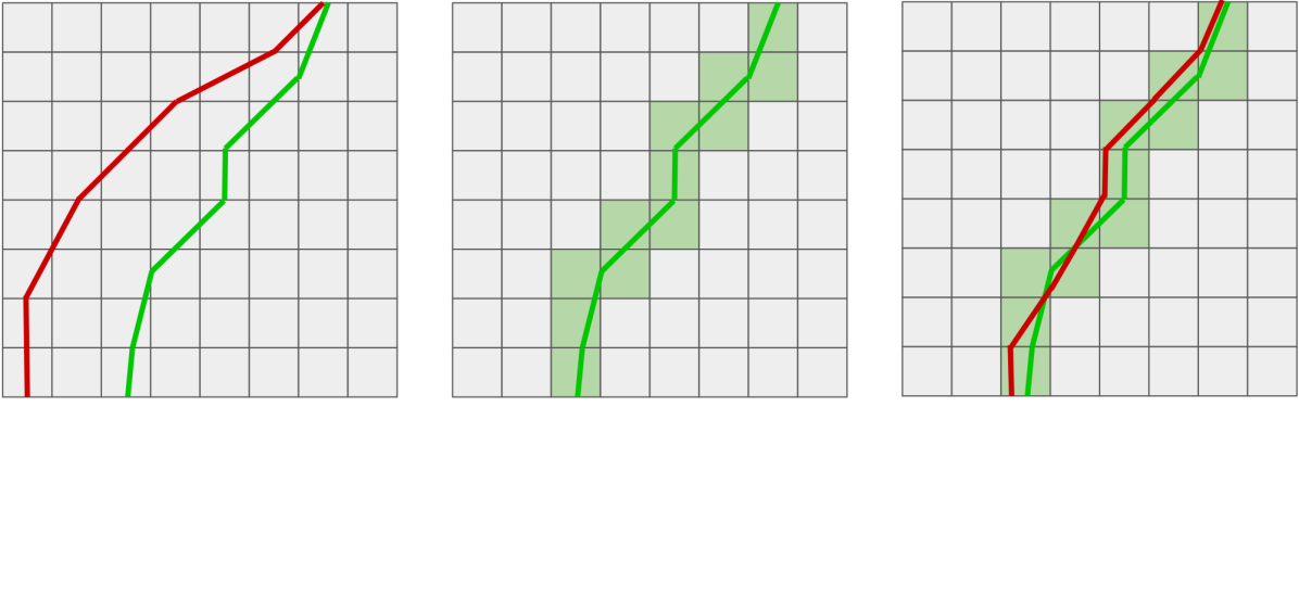
Figure 3: Topology mask in inference: We illustrate a 2D slice from a block, where each cell represents a voxel. (left) Without masking, the reconstructed surface (red) deviates from the ground truth (green) because of compression error. (mid) Losslessly compressed signs will give us ground truth occupancy/topology during inference. (right) Therefore, the average reconstructed error due to lossy magnitude compression is bounded by the size of a voxel ($5$mm).

4.2 Training

We learn the parameters $\Theta{=}\{\bm{\theta}_{e},\bm{\theta}_{s},\bm{\theta}_{d},\bm{\phi}\}$ of our compression model by minimizing the following objective

$$\operatorname*{arg\,min}_{\Theta}\>\underbrace{D_{\hat{\bm{x}}}(\bm{x},\hat{\bm{x}};\bm{\theta}_{e},\bm{\theta}_{d})}_{\text{distortion}}+\lambda[\underbrace{R_{\hat{\mathbf{z}}}(\hat{\mathbf{z}};\bm{\phi})}_{\text{latents bitrate}}+\underbrace{R_{\mathbf{s}}(\mathbf{s};\bm{\theta}_{s})}_{\text{signs bitrate}}]$$ (1)

Distortion $\bm{D_{\hat{\bm{x}}}(\bm{x},\hat{\bm{x}};\bm{\theta}_{e},\bm{\theta}_{d})}$

We minimize the reconstruction error between the ground truth and the predicted TSDF values. However, directly computing the squared difference $\|\hat{\bm{x}}~{}{-}~{}\bm{x}\|_{2}^{2}$ wastes model complexity on learning to precisely reconstruct values of TSDF voxels that are far away from the surface. In order to focus the network on the important voxels (i.e. the ones with a neighboring voxel of opposing sign), we use the ground truth signs. For each dimension, we create a mask of important voxels, namely $m_{x}$, $m_{y}$ and $m_{z}$. Voxels that have more than one neighbor with opposite signs appear in multiple masks, further increasing their weights. We then use these masks to calculate the squared differences for important voxels only $D_{\hat{\bm{x}}}=\tfrac{1}{B}\sum_{n=1}^{B}\sum_{d\in{x,y,z}}\|m_{d}\cdot(\hat{\bm{x}}_{n}-\bm{x}_{n})\|_{2}^{2},$ for $B$ blocks.

Rate of latents $\bm{R_{\hat{\mathbf{z}}}(\hat{\mathbf{z}};\bm{\phi})}$

A second loss term we employ is $R_{\hat{\mathbf{z}}}$, which is designed to reduce the bitrate of the compressed codes. This loss is essentially a differentiable estimate of the non-differentiable Shannon entropy of the quantized codes $\hat{\mathbf{z}}$; see [2] for additional details.

Rate of losslessly compressed signs $\bm{R_{\mathbf{s}}(\mathbf{s};\bm{\theta}_{s})}$

Since $\mathbf{s}$ contains only discrete values $\{-1,+1\}$, it can be compressed losslessly using entropy coding. As mentioned above, we use the conditional probability distribution $p_{\mathbf{s}|\hat{\mathbf{z}}}(\mathbf{s}|\hat{\mathbf{z}})$ instead of the prior distribution $p_{\mathbf{s}}(\mathbf{s})$. Note that the conditional distribution should have a much lower entropy than the priors, since $\mathbf{s}$ is dependent on the $\hat{\mathbf{z}}$ by design. This allows us to compress the signs far more efficiently.

To make this dependency explicit, we add an extra head to the decoder, such that $p_{\mathbf{s}}(\mathbf{s}|\hat{\mathbf{z}}){=}\mathcal{D}_{s}(\hat{\mathbf{z}})$, and $\hat{\bm{x}}{=}\mathbf{s}\odot|\mathcal{D}_{b}(\hat{\mathbf{z}})|$. The sign rate loss $R_{\mathbf{s}}$ is then the cross entropy between the ground truth signs $\mathbf{s}$, with $-1$ remapped to $0$, and their conditional predictions $p_{\mathbf{s}}(\mathbf{s}|\hat{\mathbf{z}})$. Minimizing $R_{\mathbf{s}}$ has the effect of training the network to make better sign predictions, while also minimizing the bitrate of the compressed signs.

Encoder and Decoder architectures

Our proposed compression technique is agnostic to the choice of the individual architectures for the encoder and decoder. In this work, we targeted a scenario requiring a maximum model size of roughly 2MB, which makes the network suitable for mobile deployment. To limit the number of trainable parameters, we used convolutional networks, where both the encoder and the decoder consist of a series of 3D convolutions and transposed convolutions. More details about the specific architectures can be found in the supplementary material.

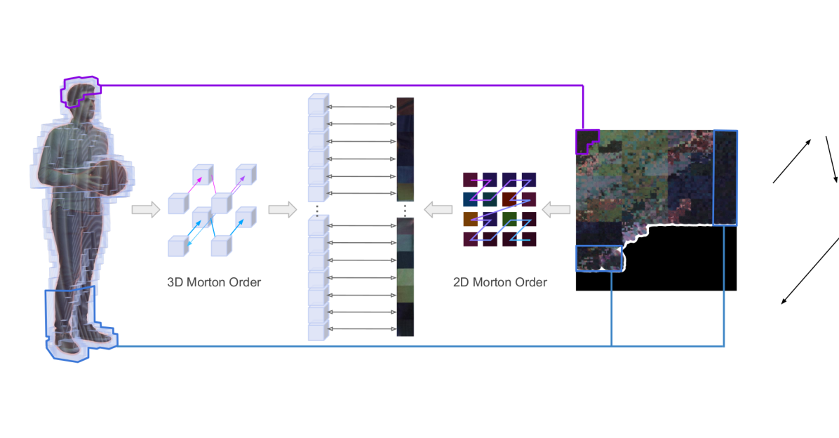
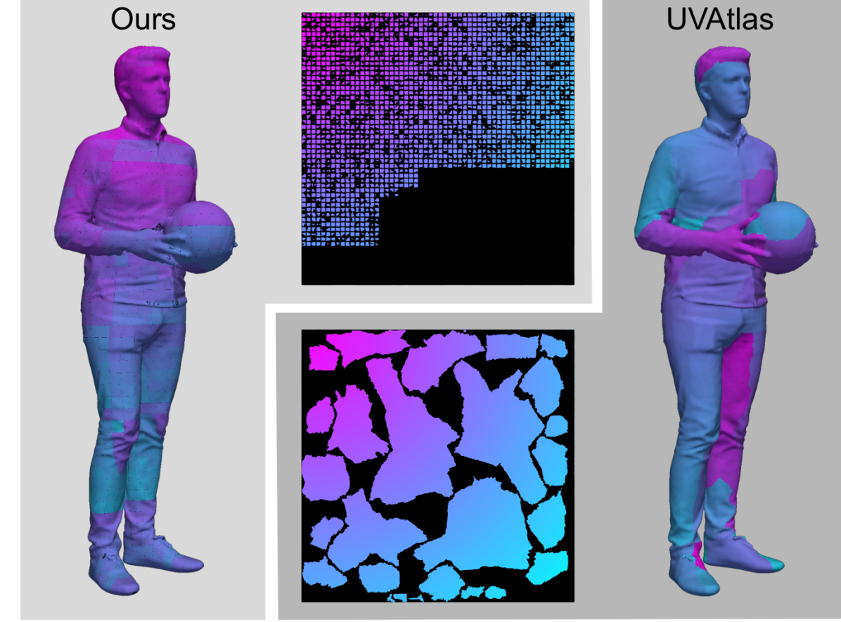
Figure 4: Texture packing – (left) 3D blocks and 2D patches are ordered and matched by their Morton codes respectively. This process unwraps the 3D volume to the texture atlas. (right) The UVAtlas [71] only ensures local spatial coherence within each chart, whilst our method encourages global spatial coherence. Refer to the supplementary video for a comparison on temporal coherence.

5 Texture compression

We propose a novel efficient and tracking-free UV parametrization method to be seamlessly combined with our block-level geometry compression; see Figure 2. As our parametrization process is deterministic, UV coordinates can be inferred on the receiver side, thus removing the need for compression and transmission of the UV coordinates.

Block-level charting

Traditional UV mapping either partitions the surface into a few large charts [71], or generates one chart per triangle to avoid UV parametrization as in PTEX [6]. In our case, since the volume has already been divided into fixed-size blocks during geometry compression, it is natural to explore block-level parametrization. To accommodate compression error, the compressed signal is decompressed on the sender side, such that both the sender and receiver have access to identical reconstructed volumes; see Figure 2 (left). Triangles of each occupied block are then extracted and grouped by their normals. Most blocks have only one group, while blocks in more complex areas (e.g. fingers) may have more. The vertices of the triangles in each group are then mapped to UV space as follows: \raisebox{-.6pt}{1}⃝ the average normal in the group is used to determine a tangent space, onto which the vertices in the group are projected; \raisebox{-.6pt}{2}⃝ the projections are rotated until they fit into an axis-aligned rectangle with minimum area, using rotating calipers [63]. This results in deterministic UV coordinates for each vertex in the group relative to a bounding box for the vertex projections; \raisebox{-.6pt}{3}⃝ the bounding boxes for the groups in a block are then sorted by size and packed into a chart using a quadtree-like algorithm. There is exactly one 2D chart for each occupied 3D block. After this packing, the UV coordinates for the vertices in the block are offset to be relative to the chart. These charts are then packed into an atlas, where the UV coordinates for the vertices are again offset to be relative to the atlas, i.e. to be a global UV mapping. After UV parametrization, color information can be obtained from either per-vertex color in the geometry, previously generated atlas or even raw RGB captures. Our method is agnostic to this process.

Morton packing

In order to optimize compression, the block-level charts need to be packed into an atlas in a way that maximizes spatio-temporal coherence. This is non-trivial, as in our sparse volume data structure the amount and positions of blocks can vary from frame to frame. Assuming the movement of the subject is smooth, preserving the 3D spatial structure among blocks during packing is expected to preserve spatio-temporal coherence. To achieve this effect we propose a Morton packing strategy. Morton ordering [43] (also called Z-order curve) has been widely used in 3D graphics to create spatial representations [33]. As our blocks are on a 3D regular grid, each occupied block can be indexed by a triple of integers $(x,y,z){\in}\mathbb{Z}^{3}$. Each integer has a binary representation, e.g. $x_{B-1}\cdots x_{0}$, where $x{=}\sum_{b=0}^{B-1}x_{b}2^{b}$. The 3D Morton code for $(x,y,z)$ is defined as the integer $\mathbf{M}_{3}(x,y,z){=}\sum_{b=0}^{B-1}(4y_{b}+2x_{b}+z_{b})2^{3b}$ whose binary representation consists of the interleaved bits $y_{B-1}x_{B-1}z_{B-1}\cdots y_{0}x_{0}z_{0}$. Likewise, as our charts are on a 2D regular grid, each chart can be indexed by a pair of integers $(u,v){\in}\mathbb{Z}^{2}$, whose 2D Morton code is the integer $\mathbf{M}_{2}(u,v){=}\sum_{b=0}^{B-1}(2u_{b}+v_{b})2^{2b}$ whose binary representation is $u_{B-1}v_{B-1}\cdots u_{0}v_{0}$. These functions are invertible simply by demultiplexing the bits. We map the chart for an occupied block at volumetric position $(x,y,z)$ to atlas position $(u,v){=}\mathbf{M}_{2}^{-1}(rank(\mathbf{M}_{3}(x,y,z)))$, where $rank$ is the rank of the 3D Morton code in the list of 3D Morton codes, as illustrated in Figure 4 (left). Note that we choose to prioritize $y$ over $x$ and $z$ when interleaving their bits into the 3D Morton code, as $y$ is the vertical direction in our coordinate system, to accommodate typically standing human figures. Hence, as long as blocks move smoothly in 3D space, corresponding patches are likely to move smoothly in the atlas, leading to an approximate spatio-temporal coherence, and therefore better (video) texture compression efficacy.

6 Evaluation

To assess our method, we rely on the dataset captured by Tang et al. [59], which consists of six ${\sim}500$ frames long RGBD multi-view sequences of different subjects at $30$Hz. We use three of them for training and the others for evaluation. We also employ “The Relightables” dataset by Guo et al. [26], which contains higher quality geometry and higher resolution texture maps – three ${\sim}600$-frame sequences. To demonstrate the generalization of learning-based methods, we only train on the dataset Tang et al. [59], and test on both  Tang et al. [59] and Guo et al. [26].

6.1 Geometry compression

We evaluate geometry compression using two different metrics: the Hausdorff metric ($\mathbf{H}$) [11] measures the ($\max$) worst-case reconstruction error via:

$$\mathbf{H}(\mathcal{S},\mathcal{\hat{S}})=\max\left(\max_{x\in\mathcal{S}_{v}}d(x,\mathcal{\hat{S}}),\max_{y\in\mathcal{\hat{S}}_{v}}d(y,\mathcal{S})\right),$$ (2)

where $\mathcal{S}_{v}$ and $\mathcal{\hat{S}}_{v}$ are the set of points on the ground truth and decoded surface respectively. $d(\mathbf{x},\mathcal{S})$ is the shortest Euclidean distance from a point $\mathbf{x}{\in}\mathbb{R}^{3}$ to the surface $\mathcal{S}$. Another metric is the symmetric Chamfer distance ($\mathbf{C}$):

$$\mathbf{C}(\mathcal{S},\mathcal{\hat{S}})=\tfrac{1}{2|\mathcal{S}_{v}|}\sum_{x\in\mathcal{S}_{v}}d(x,\mathcal{\hat{S}})+\tfrac{1}{2|\mathcal{\hat{S}}_{v}|}\sum_{y\in\mathcal{\hat{S}}_{v}}d(y,\mathcal{S}).$$ (3)

For each metric, we compute a final score averaging all volumes, which we refer to as Average Hausdorff Distance and Average Chamfer Distance respectively.

	Raw data	Naïve	Ours
Avg. Size / Volume	155.1KB	139.8KB	2.9KB

Table 1: Lossless sign compression: Our data-driven probability model, combined with an arithmetic coder, can improve the compression rate by 48$\times$ comparing to a naïve probabilty model based on statistics of signs in the dataset.

Signs

We showcase the benefit of our data dependent probability model on rate in Table 1. Raw sign data, though being binary, has an average size of $154.1$KB per volume. With naïvely computed probability of signs being positive over the dataset, an arithmetic coder can slightly improve the rate to $139.8$ KB. This is because there are more positive TSDF values than negative in the dataset. With our learned, data dependent probability model, the arithmetic coder can drastically compress the signs down to $2.9$ KB per volume.

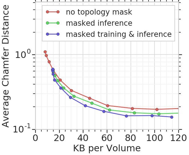
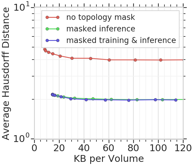
Figure 5: Topology Mask: When topology masking is applied during inference, an upper bound of error is guaranteed. Moreover, when also applied as a training loss, topology mask yields better rate-distortion. The difference is more obvious with the Hausdorff distance, which measures the worst case error.

Topology Masking

To demonstrate the impact of utilizing ground truth sign/topology, we construct a baseline with a standard rate-distortion loss. Specifically, the distortion term is simplified as $D_{\hat{\bm{x}}}{=}\tfrac{1}{B}\sum_{n=1}^{B}\|\hat{\bm{x}}_{n}-\bm{x}_{n}\|_{2}^{2}.$ This baseline is shown as no topology mask in Figure 5. Without the error bound, its distortion is much higher than other baselines. The second baseline, in addition to using the same distortion term, losslessly compresses and streams the signs during inference, as described in Section 4. Despite the increased rate due to losslessly compressed signs, this baseline still achieves better rate-distortion trade-off. Finally, using topology masking in both training and inference yields the best rate-distortion performance.

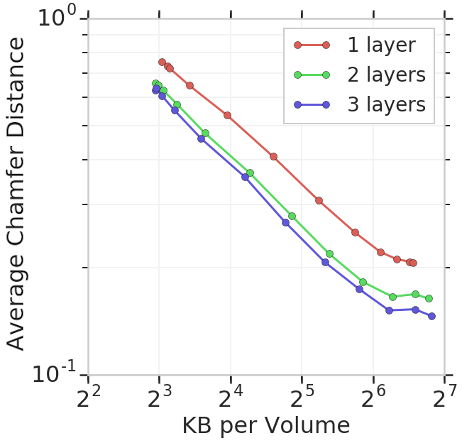
(a) Number of layers.

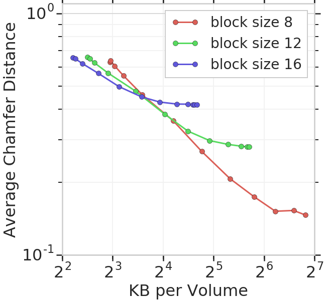
(b) Different block sizes.

Figure 6: Ablation studies: (a) Larger number of layers in both the encoder and the decoder improves performance, although with diminishing returns and increasing model size. (b) Larger block size performs better at low rates, while smaller blocks achieve better trade-off at higher rates.

Ablation studies

The impact of network architecture on compression is evaluated in Figure 6. While having more layers leads to better results, there are diminishing returns. To keep the model size practical, we restricted our model to three layers (${<}1.8$MB). We also perform ablation for the block-size (voxels/block). Since in all volumes, the voxel size is $5$ mm, a block with block-size $8^{3}$ has the physical size of $40\text{mm}^{3}$. Note that increasing the size of each block reduces the number of blocks. Results show that if one has a budget of more than $12$ KB per volume, using block size $8^{3}$ yields much better rate-distortion performance. Therefore in the following experiments, $\times 3$ layers with $8^{3}$ blocks is used.

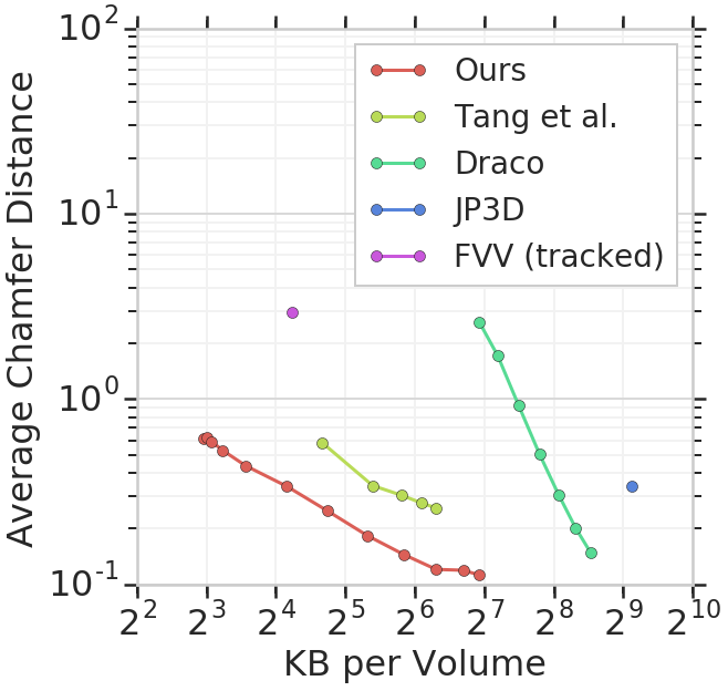
(a) Dataset Tang et al. [59]

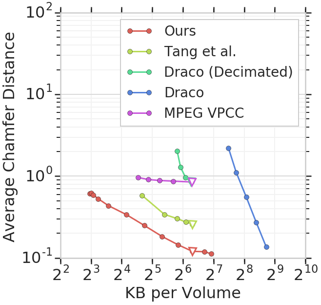
(b) Dataset Guo et al. [26]

Figure 7: Quantitative comparisons – Our method yields the best rate-distortion among state-of-the-arts. Data points marked with $\triangledown$ are selected to have similar rates and whose distortion is visualized qualitatively in Figure 10.

State-of-the-art comparisons

We compare with state-of-the-art geometry compression methods, including two volumetric methods: Tang et al. [59] and JP3D [55]; two mesh compression: Draco [24] and Free Viewpoint Video (FVV) [13]; as well as a point cloud compressor MPEG VPCC [57]. See their parameters in the supplementary material. For most of the methods, we sweep the rate hyper parameter to generate rate-distortion curves. The dataset [26] contains high-resolution meshes (${\sim}250$K vertices), which has a negative impact on the Draco compression rate. Hence, for Draco only, we decimate the meshes to 25K vertices termed as Draco (decimated) to make it comparable to other methods. Figure 7 shows that on both datasets, our method significantly outperforms all prior art in both rate and distortion. For instance, to achieve the same level of rate (marked with $\triangledown$ in Figure 7 (b)), the distortion of our method ($0.12$) is $50\%$ of Tang et al. [59] ($0.25$), and $14\%$ of Draco (decimated) ($0.86$) and MPEG ($0.84)$. To achieve the same distortion level ($0.25$), our method ($26$KB) only requires $33\%$ of the previous best performing method Tang et al. [59] ($79$KB).

To showcase difference in distortion, we select a few qualitative examples with similar rates, and visualize them in Figure 10: the Draco (decimated) results are low-res, the MPEG V-PCC results are noisy, while the results of Tang et al. [59] suffer blocking artifacts.

Efficiency

To assess the complexity of our neural network, we measure the runtime of the encoder and the decoder. We freeze our graph and run it using the Tensorflow C++ interface on a single NVIDIA PASCAL TITAN Xp GPU. Our range encoder implementation is single-threaded CPU code, hence we include only the neural network inference time. We measure 20 ms to run both encoder and decoder on all the blocks of a single volume.

Figure 8: Geometry / Qualitative – Examples from the Guo et al. [26] dataset with different rates. (1st row) Decompressed meshes. (2nd row) Shortest distance from decompressed vertices to ground truth surface. Distance between $[0,2.5\text{mm}]$ is mapped to $[0,255]$ on the red channel.

6.2 Texture compression

We compare our texture parametrization to UVAtlas [71]. In order to showcase the benefit of Morton packing, we also have a block-based baseline where naïve bin packing is used without any spatio-temporal coherence, as shown in Table 2. To preserve the high quality of the target dataset  [26], we generate high-res texture maps (4096x4096) for all experiments. The texture maps of each sequence are compressed with the H.264 implementation from FFMpeg with default parameters. Per-frame compressed sizes of different methods are reported to showcase how texture parametrization impacts the compression rate. In order to measure distortion, each textured volume with its decompressed texture atlas is rendered into the viewpoints of RGB cameras that were used to construct the volumes, and compared with the corresponding raw RGB image. For simplicity we only select 10 views (out of 58) where the subject face is visible. When computing distortion, masks are used to ensure only foreground pixels are considered, as shown in Figure 9.

Method	Rate	PSNR	SSIM	MS-SSIM
UVAtlas [71]	457	30.9	0.923	0.939
Ours (Naïve)	529	30.9	0.924	0.939
Ours (Morton)	350	30.9	0.924	0.940

Table 2: Texture / Quantitative – Average KB per volume from video compression is reported as Rate. With negligible difference in distortion under different metrics (PSNR, SSIM [67] and MS-SSIM [66]), our method preserves better spatio-temporal coherence and thus has better compression rate. See qualitative results in the supplementary video.

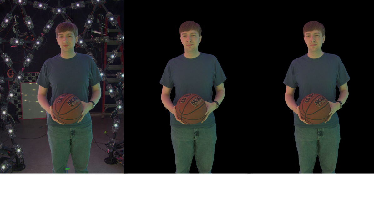
Figure 9: Texture / Qualitative – A frame taken from the comparison sequences in the supplementary video: (left) raw rgb image from camera; (mid) rendered with UVAtlas [71]; (right) rendered with our texture atlas. there is no visible difference in quality.

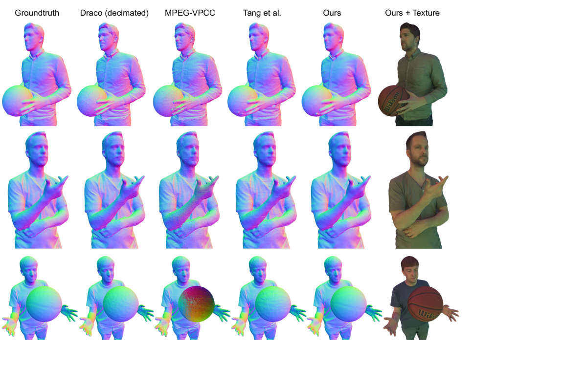
Figure 10: Qualitative vs. State-of-the-art – Examples are selected to have a similar rate but different distortions, which correspond to the markers in Figure 7 (right) – flat Phong shading is used in all cases to reveal artifacts. In order to achieve the same level of bitrate as other methods, Draco requires decimating input, which results in low-poly reconstruction. MPEG-VPCC only compresses point clouds. Tang et al. [59] has visible block artifact. Our method achieves the best distortion.

7 Conclusions

We have introduced a novel system for the compression of TSDFs and their associated textures achieving state-of-the-art results. For geometry, we use a block-based learned encoder-decoder architecture that is particularly well suited for the uniform 3D grids typically used to store TSDFs. To train better, we present a new distortion term to emphasize the loss near the surface. Moreover, ground truth signs of the TSDF are losslessly compressed with our learned model to provide an error bound during decompression. For texture, we propose a novel block-based texture parametrization algorithm which encourages spatio-temporal coherence without tracking and the necessity of UV coordinate compression. As a result, our method yields a much better rate-distortion trade-off than prior art, achieving $50\%$ distortion, or when distortion is fixed, $33\%$ bitrate of Tang et al. [59].

Future work

There are a number of interesting avenues for future work. In our architecture, we have assumed blocks to be i.i.d., and dropping this assumption could further increase the compression rate – for example, one could devise an encoder that is particularly well suited to compress “human shaped” geometry. Further, we do not make any use of temporal consistency in 4D sequences, while from the realm of video compression we know coding inter-frame knowledge provides a very significant boost to compression performance. Finally, while our per-block texture parametrization is effective, it is not included in our end-to-end training pipeline – one could learn a per-block parametrization function to minimize screen-space artifacts.

Deep Implicit Volume Compression
(Supplementary Material)

Danhang Tang  Saurabh Singh  Philip A. Chou  Christian Häne  Mingsong Dou
Sean Fanello  Jonathan Taylor  Philip Davidson  Onur G. Guleryuz  Yinda Zhang
Shahram Izadi  Andrea Tagliasacchi  Sofien Bouaziz  Cem Keskin
Google

8 Background on compression

Truncated Signed Distance Fields

A surface $\mathcal{S}$ represented in TSDF implicit form is the zero crossing of a function $\Phi(\bm{x}){:}\mathbb{R}^{3}{\rightarrow}\mathbb{R}$ that interpolates a uniform ${W{}{\times}H{}{\times}D}{}$ 3D grid of truncated (and signed) distances from the surface. By convention, distances outside and inside the surface get positive and negative signs respectively, and magnitudes are truncated by a threshold value $\tau$. Typically a method like marching cubes [37] is used to determine the topology of each voxel (i.e. which voxel edges intersect with the surface), as well as the offsets of the intersection points for the valid edges, which are then used to form a triangular mesh.

Lossless compression

The primary goal of general purpose lossless compression is to minimize the storage or transmission costs (typically measured in bits) of a discrete dataset $\mathcal{X}=(\bm{x}_{1},\ldots,\bm{x}_{N})$. Each data point of $\mathcal{X}$ is mapped to a variable length string of bits for storage or transmission by the sender. A receiver then inverts the mapping to recover the original data from the transmitted bits. The Shannon entropy $H{=}-\sum_{\bm{x}}p_{\bm{x}}(\bm{x})\log p_{\bm{x}}(\bm{x})$ provides an achievable lower bound on the rate, i.e. the minimum expected number of bits required to encode an element, where $p_{\bm{x}}(\bm{x})$ is the underlying distribution of $\bm{x}$. This is achievable by encoding $\bm{x}$ to a bit string of length $-\log p_{\bm{x}}(\bm{x})$ bits. Although this length is not necessarily an integer, it can be achieved arbitrarily closely on average by an arithmetic coder [14]. With this encoding, the number of bits needed to code the entire dataset is

$$R(\mathcal{X})=-\tfrac{1}{N}\sum_{i=1}^{N}\log p_{\bm{x}}(\bm{x}_{i}),$$ (4)

where $R$ is referred to as the bit rate of the compression.

Lossy compression

In contrast, lossy compression methods can achieve significantly higher compression rates by allowing errors in the received data. These errors are typically referred to as distortion $D$. In lossy compression there is a fundamental compromise between the distortion $D$ and the bit rate $R$, referred to as rate-distortion trade–off, where distortion can be decreased by spending more bits. Minimizing $D$ subject to a constraint on $R$ leads to the following unconstrained optimization problem [9, 46]

$$\operatorname*{arg\,min}_{\hat{\bm{x}}}D(\bm{x},\hat{\bm{x}})+\lambda R(\hat{\bm{x}}),$$ (5)

where $\hat{\bm{x}}$ is a discrete lossy representation of $\bm{x}$ and $\lambda$ is a trade–off parameter. Higher values of $\lambda$ result in better bit rates at the expense of increased distortion.

Lossy transform coding

Often $\bm{x}$ is high dimensional, making the direct optimization of the problem above intractable. As a result, lossy transform coding is more commonly used instead. In lossy transform coding, a transformation is used to transform the original data $\bm{x}$ into a latent representation $\mathbf{z}{=}\mathcal{E}(\bm{x};\bm{\theta}_{e})$ and another is used to approximately recover the original data $\hat{\bm{x}}{=}\mathcal{D}(\hat{\mathbf{z}};\bm{\theta}_{d})$ from the lossy latent representation $\hat{\mathbf{z}}$. The transformations $\mathcal{E}$ and $\mathcal{D}$, with parameters $\bm{\theta}_{e}$ and $\bm{\theta}_{d}$, respectively, are typically chosen to simplify the conversion from $\mathbf{z}$ to its lossy discrete version $\hat{\mathbf{z}}{=}Q(\mathbf{z})$ – a process called quantization. While $\mathcal{E}$ and $\mathcal{D}$ can be invertible transformations (e.g. the discrete cosine transform used for JPEG compression), in general they are not required to be. Thus, with $\bm{\theta}{=}\{\bm{\theta}_{e},\bm{\theta}_{d}\}$, the original rate-distortion problem can be re-written as

$$\operatorname*{arg\,min}_{\bm{\theta},\bm{\phi}}\>\>D(\bm{x},\hat{\bm{x}};\bm{\theta})+\lambda R(\hat{\mathbf{z}};\bm{\phi}),$$ (6)

where $\hat{\bm{x}}{=}\mathcal{D}(\hat{\mathbf{z}};\bm{\theta}_{d})$, $\hat{\mathbf{z}}{=}Q(\mathcal{E}(\bm{x};\bm{\theta}_{e}))$, and the bit rate is $R(\hat{\mathbf{z}};\bm{\phi}){=}{-}\log p_{\hat{\mathbf{z}}}(\hat{\mathbf{z}};\bm{\phi})$, with $p_{\hat{\mathbf{z}}}$ as a probability model of $\hat{\mathbf{z}}$ with parameters $\bm{\phi}$ that is learned jointly with $\bm{\theta}$. The code $\hat{\mathbf{z}}$ is converted to the corresponding variable length bit representation by entropy coding using the learned prior distribution $p_{\hat{\mathbf{z}}}$.

Method	Rate Parameters (varied)	Fixed Parameters
Ours	$\lambda=\frac{1}{10^{\mu}},\mu=i\times\frac{\log_{10}200000}{11}$ (for $i=0,\dots 11$)
Tang et al. [59]	$K_{total}=1024,2048\ldots 5120$	$\text{numRetainedKLTBases}=64$
Google Draco [24]	$\text{qp}=8,\ldots,11$	$\text{qt}=11$ $\text{skip}=\text{normal}$
MPEG V-PCC [57]	r$i$ configurations (for $i=1,\ldots,5$)	$\text{geometry3dCoordinatesBitdepth}=11$ $\text{geometryNominal2dBitdepth}=8$ $\text{minNormSumOfInvDist4MPSelection}=0.36$ $\text{partialAdditionalProjectionPlane}=0.15$ $\text{minimumImageWidth}=2560$ $\text{apply3dMotionCompensation}=0$

Table 3: Parameters used for the experiments in Figure 7 of the main paper.

Quantization

Since the quantization operation is non-differentiable, training such a network in an end-to-end fashion is challenging. Ballé et al. [2] propose simulating quantization noise during training rather than explicitly discretizing the code. Specifically, they quantize $\mathbf{z}$ by rounding to nearest integer $\hat{\mathbf{z}}{=}Q(\mathcal{E}(\bm{x};\bm{\theta}_{e})){=}\lfloor\mathcal{E}(\bm{x};\bm{\theta}_{e})\rceil$, which they model by adding of uniform noise during training, i.e. $\hat{\mathbf{z}}{=}\mathcal{E}(\bm{x};\bm{\theta}_{e}){+}\epsilon$, $\epsilon{~{}}\sim~{}\mathcal{U}[-0.5,0.5]$ to simulate quantization errors; see [2] for additional details.

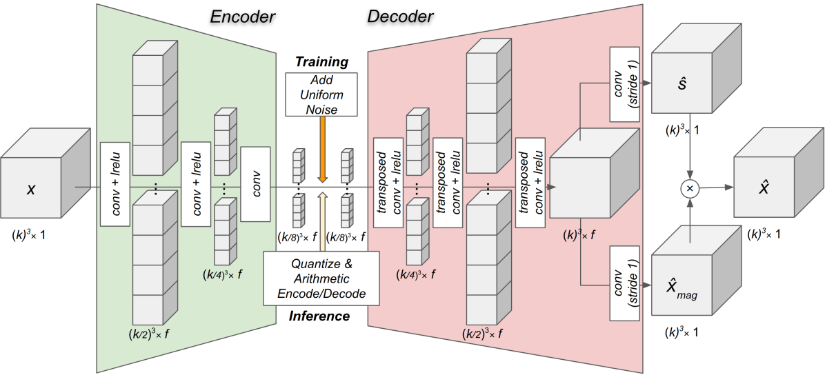
Figure 11: Network architecture. The encoder $\mathcal{E}$ consists of three convolutional layers and the decoder $\mathcal{D}$ has three transposed convolution layers, each with a stride of two. $\mathcal{D}$ has two convolutional heads with a stride of one, which separates sign prediction from TSDF estimation. Refer to Section 4 in main paper for details.

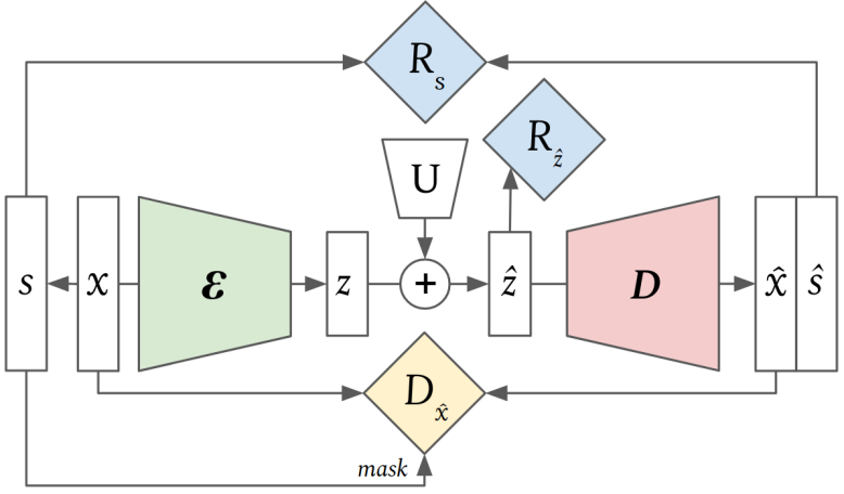
Figure 12: Training losses. During training, we employ three different losses as explained in Section 4. Here, the distortion loss $D_{\hat{\bm{x}}}$ makes use of the ground truth signs $\mathbf{s}$ to mask the voxels that have no neighboring voxels with opposing signs and have therefore less significance. $R_{\mathbf{s}}$ is the cross entropy between the predicted and actual signs, which is used to minimize the bit rate for compressed ground truth signals. $R_{\hat{\mathbf{z}}}$ is an estimate of the differential entropy of the noisy latent code, also used to minimize the bit rate for the compressed latent code $\hat{\mathbf{z}}$.

9 Network architecture and training

We visualize the architecture of our model in  Figure 11, which is formed by a three layer encoder and decoder. While the architecture is similar to a convolutional autoencoder (implemented with convolutions in the encoder and transposed convolutions in the decoder), the main difference lies in the transformation the latent code goes through, and the additional losses that aim to minimize the bit rate as well as the reconstruction error, as visualized in  Figure 12. Specifically, we add uniform noise to the code during training to simulate quantization. At test time we quantize the code and compress it with an entropy coder. Additionally, the decoder has two final convolutional heads that separate the estimation of signs and the TSDF values. The one and two layer models we experiment with are similar with fewer layers.

Figure 12 provides an overview of our training setup with the dependencies for the three terms in our training loss. Unlike a regular autoencoder which only aims to minimize the reconstruction error, we employ two additional losses $R_{\hat{\mathbf{z}}}$ and $R_{\mathbf{s}}$ to minimize the bit rates for the compressed signals for the latent code and the ground truth signs. Additionally, instead of equally weighting each element the reconstructed $\hat{\bm{x}}$, we use the ground truth signs $\mathbf{s}$ to mask the voxels that have no neighboring voxels with opposing signs and have therefore less significance.

10 Baseline parameters

The parameters used in our experiments (Figure 6) are described in Table 3, except for JP3D [55] and FVV [13] which we obtained from Tang et al. [59]. To generate a curve, we varied the corresponding rate parameter during inference, whilst keeping other parameters fixed as shown. Notations and definitions of parameters can be found in respective citations.

References

- Alliez and Gotsman [2005] P. Alliez and C. Gotsman. Recent advances in compression of 3d meshes. In N. A. Dodgson, M. S. Floater, and M. A. Sabin, editors, Advances in Multiresolution for Geometric Modeling, pages 3–26. Springer Berlin Heidelberg, Berlin, Heidelberg, 2005.
- Ballé et al. [2017] Johannes Ballé, Valero Laparra, and Eero Simoncelli. End-to-end optimized image compression. In ICLR, 2017.
- Ballé et al. [2018] Johannes Ballé, David Minnen, Saurabh Singh, Sung Jin Hwang, and Nick Johnston. Variational image compression with a scale hyperprior. ICLR, 2018.
- Botsch et al. [2010] Mario Botsch, Leif Kobbelt, Mark Pauly, Pierre Alliez, and Bruno Lévy. Polygon mesh processing. CRC press, 2010.
- Briceño et al. [2003] H. Briceño, P. Sander, L. McMillan, S. Gortler, and H. Hoppe. Geometry videos: a new representation for 3d animations. In Symp. Computer Animation, 2003.
- Burley and Lacewell [2008] Brent Burley and Dylan Lacewell. Ptex: Per-face texture mapping for production rendering. In Proceedings of the Nineteenth Eurographics Conference on Rendering, EGSR ’08, pages 1155–1164, Aire-la-Ville, Switzerland, Switzerland, 2008. Eurographics Association.
- Canelhas et al. [2017] Daniel-Ricao Canelhas, Erik Schaffernicht, Todor Stoyanov, Achim J Lilienthal, and Andrew J Davison. Compressed voxel-based mapping using unsupervised learning. Robotics, 2017.
- Carranza et al. [2003] Joel Carranza, Christian Theobalt, Marcus A. Magnor, and Hans-Peter Seidel. Free-viewpoint video of human actors. ACM Trans. Graph., 22(3):569–577, July 2003. ISSN 0730-0301.
- Chou et al. [1989] P.A. Chou, T. Lookabaugh, and R.M. Gray. Entropy-constrained vector quantization. IEEE Transactions on Acoustics, Speech, and Signal Processing, 37(1):31–42, January 1989.
- Chou et al. [2019] Philip A. Chou, Maxim Koroteev, and Maja Krivokuća. A volumetric approach to point cloud compression, Part I: Attribute compression. IEEE Trans. Image Processing, March 2019.
- Cignoni et al. [1998] Paolo Cignoni, Claudio Rocchini, and Roberto Scopigno. Metro: Measuring error on simplified surfaces. cgf, 1998.
- Cohen et al. [2016] R. A. Cohen, D. Tian, and A. Vetro. Attribute compression for sparse point clouds using graph transforms. In IEEE Int’l Conf. Image Processing (ICIP), Sept 2016.
- Collet et al. [2015] Alvaro Collet, Ming Chuang, Pat Sweeney, Don Gillett, Dennis Evseev, David Calabrese, Hugues Hoppe, Adam Kirk, and Steve Sullivan. High-quality streamable free-viewpoint video. ACM Trans. on Graphics (TOG), 2015.
- Cover and Thomas [2006] T.M. Cover and J.A. Thomas. Elements of Information Theory. John Wiley and Sons, 2006.
- Curless and Levoy [1996] B. Curless and M. Levoy. A volumetric method for building complex models from range images. In Proc. 23rd annual ACM conference on Computer graphics and interactive techniques (SIGGRAPH’96), pages 303–312, 1996.
- de Queiroz and Chou [2017] R. L. de Queiroz and P. A. Chou. Transform coding for point clouds using a Gaussian process model. IEEE Trans. Image Processing, 26(8), August 2017.
- de Queiroz and Chou [2016] Ricardo L. de Queiroz and Philip A. Chou. Compression of 3D point clouds using a region-adaptive hierarchical transform. IEEE Trans. Image Processing, 25(8), August 2016.
- d’Eon et al. [2017] E. d’Eon, B. Harrison, T. Myers, and P. A. Chou. 8i voxelized full bodies — a voxelized point cloud dataset. input documents M74006 & m40059, ISO/IEC JTC1/SC29/WG1 & WG11 JPEG & MPEG, January 2017. Available at https://jpeg.org/plenodb/pc/8ilabs/.
- Dou et al. [2015] M. Dou, J. Taylor, H. Fuchs, A. Fitzgibbon, and S. Izadi. 3d scanning deformable objects with a single rgbd sensor. In 2015 IEEE Conference on Computer Vision and Pattern Recognition (CVPR), pages 493–501, June 2015.
- Dou et al. [2016] M. Dou, S. Khamis, Y. Degtyarev, P. Davidson, S. R. Fanello, A. Kowdle, S. Orts Escolano, C. Rhemann, D. Kim, J. Taylor, P. Kohli, V. Tankovich, and S. Izadi. Fusion4d: real-time performance capture of challenging scenes. ACM Transactions on Graphics (TOG), 35(4):114, 2016.
- Dou et al. [2017a] Mingsong Dou, Philip Davidson, Sean Ryan Fanello, Sameh Khamis, Adarsh Kowdle, Christoph Rhemann, Vladimir Tankovich, , and Shahram Izadi. Motion2fusion: Real-time volumetric performance capture. ACM TOG (SIGGRAPH Asia), 2017a.
- Dou et al. [2017b] Mingsong Dou, Philip Davidson, Sean Ryan Fanello, Sameh Khamis, Adarsh Kowdle, Christoph Rhemann, Vladimir Tankovich, and Shahram Izadi. Motion2fusion: real-time volumetric performance capture. ACM Trans. on Graphics (Proc. of SIGGRAPH Asia), 2017b.
- Frisken et al. [2000] Sarah F. Frisken, Ronald N. Perry, Alyn P. Rockwood, and Thouis R. Jones. Adaptively sampled distance fields: A general representation of shape for computer graphics. In Proc. 27th Annual Conference on Computer Graphics and Interactive Techniques, SIGGRAPH ’00. ACM, 2000.
- Galligan et al. [2018] Frank Galligan, Michael Hemmer, Ondrej Stava, Fan Zhang, and Jamieson Brettle. Google/draco: a library for compressing and decompressing 3d geometric meshes and point clouds. https://github.com/google/draco, 2018.
- Gu et al. [2002] Xianfeng Gu, Steven J. Gortler, and Hugues Hoppe. Geometry images. ACM Trans. Graphics (SIGGRAPH), 21(3):355–361, July 2002. ISSN 0730-0301.
- Guo et al. [2019] Kaiwen Guo, Peter Lincoln, Philip Davidson, Jay Busch, Xueming Yu, Matt Whalen, Geoff Harvey, Sergio Orts-Escolano, Rohit Pandey, Jason Dourgarian, Danhang Tang, Anastasia Tkach, Adarsh Kowdle, Emily Cooper, Mingsong Dou, Sean Fanello, Graham Fyffe, Christoph Rhemann, Jonathan Taylor, Paul Debevec, and Shahram Izadi. The relightables: Volumetric performance capture of humans with realistic relighting. In ACM TOG, 2019.
- Izadi et al. [2011] S. Izadi, D. Kim, O. Hilliges, D. Molyneaux, R. Newcombe, P. Kohli, J. Shotton, S. Hodges, D. Freeman, A. Davison, and A. Fitzgibbon. KinectFusion: Real-time 3D reconstruction and interaction using a moving depth camera. In Proc. UIST, 2011.
- Jackins and Tanimoto [1980] C. L. Jackins and S. L. Tanimoto. Oct-trees and their use in representing three-dimensional objects. Computer Graphics and Image Processing, 14(3):249 – 270, 1980. ISSN 0146-664X.
- Kammerl et al. [2012] J. Kammerl, N. Blodow, R. B. Rusu, S. Gedikli, M. Beetz, and E. Steinbach. Real-time compression of point cloud streams. In IEEE Int’l Conference on Robotics and Automation, Minnesota, USA, May 2012.
- Kazhdan and Hoppe [2013] Michael Kazhdan and Hugues Hoppe. Screened poisson surface reconstruction. ACM Transactions on Graphics (ToG), 2013.
- Krivokuća et al. [2018] Maja Krivokuća, Maxim Koroteev, and Philip A. Chou. A volumetric approach to point cloud compression. arXiv preprint arXiv:1810.00484, 2018.
- Krivokuća et al. [submitted for possible publication] Maja Krivokuća, Philip A. Chou, and Maxim Koroteev. A volumetric approach to point cloud compression, Part II: Geometry compression. IEEE Trans. Image Processing, submitted for possible publication.
- Lauterbach et al. [2009] Christian Lauterbach, Michael Garland, Shubhabrata Sengupta, David P. Luebke, and Dinesh Manocha. Fast bvh construction on gpus. Comput. Graph. Forum, 28(2):375–384, 2009.
- Liao et al. [2018] Yiyi Liao, Simon Donné, and Andreas Geiger. Deep marching cubes: Learning explicit surface representations. In CVPR, pages 2916–2925. IEEE Computer Society, 2018.
- Loop et al. [2016a] C. Loop, Q. Cai, S. Orts Escolano, and P.A. Chou. Microsoft voxelized upper bodies — a voxelized point cloud dataset. input documents m38673/M72012, ISO/IEC JTC1/SC29/WG1 & WG11 JPEG & MPEG, May 2016a. Available at https://jpeg.org/plenodb/pc/microsoft/.
- Loop et al. [2016b] C. Loop, Q. Cai, S. Orts-Escolano, and P. A. Chou. A closed-form bayesian fusion equation using occupancy probabilities. In Int’l Conf. on 3D Vision (3DV), October 2016b.
- Lorensen and Cline [1987] William E. Lorensen and Harvey E. Cline. Marching cubes: A high resolution 3d surface construction algorithm. SIGGRAPH Comput. Graph., 21(4):163–169, August 1987. ISSN 0097-8930.
- Luttrell [1988] SP Luttrell. Image compression using a neural network. In Proc. IGARSS, volume 88, pages 1231–1238, 1988.
- Maglo et al. [2015] Adrien Maglo, Guillaume Lavoué, Florent Dupont, and Céline Hudelot. 3d mesh compression: Survey, comparisons, and emerging trends. ACM Computing Surveys (CSUR), 47(3):44, 2015.
- Mamou et al. [2009] K. Mamou, T. Zaharia, and F. Prêteux. TFAN: A low complexity 3d mesh compression algorithm. Computer Animation and Virtual Worlds, 20, 2009.
- Meagher [1982] Donald Meagher. Geometric modeling using octree encoding. Computer graphics and image processing, 19(2):129–147, 1982.
- Mekuria et al. [2017] R. Mekuria, K. Blom, and P. Cesar. Design, implementation, and evaluation of a point cloud codec for tele-immersive video. IEEE Trans. Circuits and Systems for Video Technology, 27(4):828–842, April 2017.
- Morton [1966] G. M Morton. A computer oriented geodetic data base; and a new technique in file sequencing. Technical report, IBM, Ottawa, Canada, 1966.
- Munro and Zipser [1989] PAUL Munro and DAVID Zipser. Image compression by back propagation: an example of extensional programming. Models of cognition: A review of cognitive science, 2, 1989.
- Newcombe et al. [2015] Richard A Newcombe, Dieter Fox, and Steven M Seitz. Dynamicfusion: Reconstruction and tracking of non-rigid scenes in real-time. In Proc. of Comp. Vision and Pattern Recognition (CVPR), 2015.
- Ortega and Ramchandran [1998] A. Ortega and K. Ramchandran. Rate-distortion methods for image and video compression. IEEE Signal Processing Magazine, 15(6):23–50, Nov 1998.
- Orts-Escolano et al. [2016] Sergio Orts-Escolano, Christoph Rhemann, Sean Fanello, Wayne Chang, Adarsh Kowdle, Yury Degtyarev, David Kim, Philip L Davidson, Sameh Khamis, Mingsong Dou, et al. Holoportation: Virtual 3d teleportation in real-time. In Proc. of the Symposium on User Interface Software and Technology, 2016.
- Park et al. [2019] Jeong Joon Park, Peter Florence, Julian Straub, Richard A. Newcombe, and Steven Lovegrove. Deepsdf: Learning continuous signed distance functions for shape representation. In CVPR, pages 165–174. Computer Vision Foundation / IEEE, 2019.
- Peng et al. [2005] J. Peng, Chang-Su Kim, and C. C. Jay Kuo. Technologies for 3d mesh compression: A survey. Journal of Vis. Comun. and Image Represent., 16(6):688–733, December 2005.
- Prada et al. [2017] Fabián Prada, Misha Kazhdan, Ming Chuang, Alvaro Collet, and Hugues Hoppe. Spatiotemporal atlas parameterization for evolving meshes. ACM Trans. on Graphics (TOG), 2017.
- Qi et al. [2016] Charles R. Qi, Hao Su, Kaichun Mo, and Leonidas J. Guibas. Pointnet: Deep learning on point sets for 3d classification and segmentation. In 2016 IEEE Conference on Computer Vision and Pattern Recognition (CVPR), June 2016.
- Quach et al. [2019] Maurice Quach, Giuseppe Valenzise, and Frederic Dufaux. Learning convolutional transforms for lossy point cloud geometry compression. arXiv preprint arXiv:1903.08548, 2019.
- Rossignac [1999] J. Rossignac. Edgebreaker: Connectivity compression for triangle meshes. IEEE Trans. Visualization and Computer Graphics, 5(1):47–61, Jan. 1999.
- Rusu and Cousins [2011] R. B. Rusu and S. Cousins. 3d is here: Point cloud library (PCL). In IEEE Int’l Conf. on Robotics and Automation (ICRA), pages 1–4, 2011.
- Schelkens et al. [2006] P. Schelkens, A. Munteanu, A. Tzannes, and C. Brislawn. Jpeg2000. part 10. volumetric data encoding. In 2006 IEEE International Symposium on Circuits and Systems, pages 4 pp.–3877, May 2006.
- Schnabel and Klein [2006] R. Schnabel and R. Klein. Octree-based point-cloud compression. In Eurographics Symp. on Point-Based Graphics, July 2006.
- Schwarz et al. [2018] Sebastian Schwarz, Marius Preda, Vittorio Baroncini, Madhukar Budagavi, Pablo Cesar, Philip A Chou, Robert A Cohen, Maja Krivokuća, Sébastien Lasserre, Zhu Li, et al. Emerging mpeg standards for point cloud compression. IEEE Journal on Emerging and Selected Topics in Circuits and Systems, 9(1):133–148, 2018.
- Sitzmann et al. [2019] Vincent Sitzmann, Justus Thies, Felix Heide, Matthias Nießner, Gordon Wetzstein, and Michael Zollhöfer. Deepvoxels: Learning persistent 3d feature embeddings. In CVPR, pages 2437–2446. Computer Vision Foundation / IEEE, 2019.
- Tang et al. [2018] Danhang Tang, Mingsong Dou, Peter Lincoln, Philip Davidson, Kaiwen Guo, Jonathan Taylor, Sean Fanello, Cem Keskin, Adarsh Kowdle, Sofien Bouaziz, Shahram Izadi, and Andrea Tagliasacchi. Real-time compression and streaming of 4d performances. ACM Transaction on Graphics (Proc. SIGGRAPH Asia), 2018.
- Thanou et al. [2016] D. Thanou, P. A. Chou, and P. Frossard. Graph-based compression of dynamic 3d point cloud sequences. IEEE Trans. Image Processing, 25(4), April 2016.
- Toderici et al. [2015] George Toderici, Sean M O’Malley, Sung Jin Hwang, Damien Vincent, David Minnen, Shumeet Baluja, Michele Covell, and Rahul Sukthankar. Variable rate image compression with recurrent neural networks. arXiv preprint arXiv:1511.06085, 2015.
- Touma and Gotsman [1998] Costa Touma and Craig Gotsman. Triangle mesh compression. In Proceedings of the Graphics Interface 1998 Conference, June 18-20, 1998, Vancouver, BC, Canada, pages 26–34, June 1998.
- Toussaint [1983] Godfried Toussaint. Solving geometric problems with the rotating calipers, 1983.
- Wang et al. [2019] Jianqiang Wang, Hao Zhu, Zhan Ma, Tong Chen, Haojie Liu, and Qiu Shen. Learned point cloud geometry compression. arXiv preprint arXiv:1909.12037, 2019.
- Wang et al. [2017] Peng-Shuai Wang, Yang Liu, Yu-Xiao Guo, Chun-Yu Sun, and Xin Tong. O-cnn: Octree-based convolutional neural networks for 3d shape analysis. ACM Trans. Graph., 36(4):72:1–72:11, July 2017. ISSN 0730-0301.
- Wang et al. [2003] Zhou Wang, Eero P Simoncelli, and Alan C Bovik. Multiscale structural similarity for image quality assessment. In The Thrity-Seventh Asilomar Conference on Signals, Systems & Computers, 2003, volume 2, pages 1398–1402. Ieee, 2003.
- Wang et al. [2004] Zhou Wang, Alan C Bovik, Hamid R Sheikh, Eero P Simoncelli, et al. Image quality assessment: from error visibility to structural similarity. IEEE transactions on image processing, 13(4):600–612, 2004.
- Wu et al. [2015] Zhirong Wu, Shuran Song, Aditya Khosla, Fisher Yu, Linguang Zhang, Xiaoou Tang, and Jianxiong Xiao. 3d shapenets: A deep representation for volumetric shapes. In CVPR, pages 1912–1920. IEEE Computer Society, 2015. ISBN 978-1-4673-6964-0.
- Yan et al. [2019] Wei Yan, Shan Liu, Thomas H Li, Zhu Li, Ge Li, et al. Deep autoencoder-based lossy geometry compression for point clouds. arXiv preprint arXiv:1905.03691, 2019.
- Zhang et al. [2014] C. Zhang, D. Florêncio, and C. Loop. Point cloud attribute compression with graph transform. In 2014 IEEE Int’l Conf. Image Processing (ICIP), Oct 2014.
- Zhou et al. [2004] Kun Zhou, John Synder, Baining Guo, and Heung-Yeung Shum. Iso-charts: stretch-driven mesh parameterization using spectral analysis. In Proceedings of the 2004 Eurographics/ACM SIGGRAPH symposium on Geometry processing, pages 45–54. ACM, 2004.