Sliding Basis Optimization for Heterogeneous Material Design

Abstract

We present the sliding basis computational framework to automatically synthesize heterogeneous (graded or discrete) material fields for parts designed using constrained optimization. Our framework uses the fact that any spatially varying material field over a given domain may be parameterized as a weighted sum of the Laplacian eigenfunctions. We bound the parameterization of all material fields using a small set of weights to truncate the Laplacian eigenfunction expansion, which enables efficient design space exploration with the weights as a small set of design variables. We further improve computational efficiency by using the property that the Laplacian eigenfunctions form a spectrum and may be ordered from lower to higher frequencies. Starting the optimization with a small set of weighted lower frequency basis functions we iteratively include higher frequency bases by sliding a window over the space of ordered basis functions as the optimization progresses. This approach allows greater localized control of the material distribution as the sliding window moves through higher frequencies. The approach also reduces the number of optimization variables per iteration, thus the design optimization process speeds up independent of the domain resolution without sacrificing analysis quality. While our method is useful for problems where analytical gradients are available, it is most beneficial when the gradients may not be computed easily (i.e., optimization problems coupled with external black-box analysis) thereby enabling optimization of otherwise intractable design problems. The sliding basis framework is independent of any particular physics analysis, objective and constraints, providing a versatile and powerful design optimization tool for various applications. We demonstrate our approach on graded solid rocket fuel design and multi-material topology optimization applications and evaluate its performance.

1 Introduction

Multi-material (heterogeneous) structures show great potential for superior product performance compared to homogeneous material designs. The advantages of heterogeneous material structures such as fiber reinforced, metal matrix, and ceramic matrix composites are already clear with several applications in aerospace engineering, construction, transportation, medical, and defense industries. In some applications (such as spacecraft engineering) where traditional composite materials may fail prematurely via delamination and other mechanisms, functionally graded materials characterized by gradual transitions in material compositions and microstructure can improve performance by improving mechanical properties and avoiding hard interfaces between materials.

Realizing this potential, a variety of multi-material AM technologies have been developed for different material types including polymers [1], metals [2] and ceramics [3]. These multi-material AM technologies are becoming commercially available and are being used in real world applications  [4]. However, design tools that can take full advantage of such manufacturing capabilities are missing. Manually designing heterogeneous material structures is a difficult and tedious task even for experienced engineers and designers because multi-material AM technologies can enable voxel-level control and therefore create a vast design space. For example consider a heterogeneous material design problem with $m$ discrete materials in a discretized domain with $n_{e}$ elements; the resulting design space has $n_{e}^{m}$ possible combinations of materials that may be distributed. The combinatorics are intractable very quickly even for low-resolution three dimensional heterogeneous discrete materials with voxel level control. When reasoning about weighted combinations of materials there are infinitely many combinations per voxel. The advantages of heterogeneous graded materials in aerospace and defense applications with complex interacting physics further implies the design space exploration must be efficiently coupled with domain-specific solvers to synthesize novel heterogeneous material designs.

In this paper, we present a novel method for optimizing heterogeneous material distributions given a prescribed set of design goals (Figure 1). In particular, we address inverse problems where the objective and constraints are coupled with a ‘black-box’ physical analysis whose implementation details are unknown. Our approach may be contrasted with the prominent automated synthesis technique of topology optimization [5]. Typically, topology optimization approaches rely on the idea that gradients related to simulation variables can be computed analytically. While these analytical gradients and corresponding adjoint variables are well defined for a certain set of problems such as simple linear elasticity problems, deriving analytical gradients may be problematic or costly for applications involving complex multi-physics especially when depending on external solvers for the analysis. Often, such external analysis tools do not provide the analytical gradient components that are essential in the traditional topology optimization processes.

When analytical gradients are not available, optimization approaches either use numerical gradients or employ stochastic sampling methods such as genetic algorithms [6] or simulated annealing [7]. These approaches do not scale well with increasing number of optimization variables i.e., the size of the material distribution field, because the introduction of new optimization variables requires additional analysis calls. We address this challenge by using a reduced order approach that controls the material distribution in a high-resolution analysis domain with a small number of design parameters. The key underlying idea is that any heterogeneous material field $\boldsymbol{\mathcal{F}}$ viewed as a function over a compact domain $\Omega$ can be parameterized as a weighted combination of the eigenfunctions of the Laplace operator $\Delta=\nabla\cdot\nabla$ defined over $\Omega$ (with Dirichlet boundary conditions). Every Laplacian eigenfunction $f$ satisfies the relation $\Delta f=-\lambda f$, and the set of all such $\Omega$-specific Laplacian eigenfunctions form a complete orthonormal basis $\{\boldsymbol{e_{i}}\}$ for the function space $L^{2}(\Omega)$. Therefore we may write

$$\boldsymbol{\mathcal{F}}=\sum_{i}\boldsymbol{w_{i}}\boldsymbol{e_{i}}.$$ (1)

In our approach, the design variables are the weights $\boldsymbol{w_{i}}$ applied to the pre-computed $\boldsymbol{e_{i}}$ for a given $\Omega$. In a discrete representation of $\Omega$ (e.g. as a mesh) there are finitely many $\boldsymbol{e_{i}}$ determined by the number of mesh elements. Using the eigenfunction expansion and treating weights $\boldsymbol{w_{i}}$ as design variables, we see there are as many design variables as the size of the material field (mesh elements), so this expansion simply amounts to a basis change. However, the power of the eigenfunction expansion emerges when we truncate the basis to create a much smaller set of optimization variables compared to the size of the field in the discretized $\Omega$. The $\boldsymbol{e_{i}}$ have the spectral property [8], i.e. they form a spectrum and can be ordered from low to high frequencies, and the higher frequency eigenfunctions have support over very small features. Truncating the number of basis elements removes high frequency eigenfunctions from the material field parameterization, so the computational advantage of reducing the design variables (weights) at the expense of local material field variation must be traded off carefully. Our goal is to arrive at a truncation that is sufficient to parameterize and represent the material field that optimizes the given objective and constraints.

To avoid the trial and error in selecting a smaller set of basis functions to efficiently explore the design space, we introduce the sliding basis optimization. The key observation we make in this work is that the spectral properties of the Laplacian eigenfunction basis allows us to capture material field variation over increasingly local features by sliding (i.e. incrementally moving) towards the higher frequency basis functions as the optimization progresses. Our method can be used with both numerical gradients and stochastic optimization approaches incorporating commodity optimizers. The method provides a flexible and powerful mechanism for material distribution design that can be easily applied to a variety of problems. We demonstrate two example applications. First, we apply it to graded solid rocket fuel design such that the optimized fuel distribution results in the target thrust profile when it burns. Second, we show its performance on multi material topology optimization problem where the objective is to minimize the compliance of the resulting design. For both applications, the analysis component is treated as black-box to demonstrate the effectiveness of the approach.

The main contributions of the presented work are:

• an optimization technique we call sliding basis optimization to explore parameterized design space efficiently and utilize minimal set of basis to achieve design requirements,

• application of the spectral Laplacian basis to practical material design problems with prescribed material bounds,

• enabling optimization of material distributions for new applications coupled with black-box analysis .

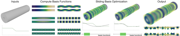
Figure 1: Overview of our approach. Given an input domain and target goals (e.g. thrust profile when designing a graded material solid rocket fuel), our algorithm optimizes the material distribution in the domain to find a configuration that matches the target goals. In the preprocessing step, we compute the Laplacian basis functions on the input domain. Then, our sliding basis optimizer adjusts the weights of a small number of active basis functions at a time. As the optimization progresses, we slide the active set towards the higher frequencies until convergence is achieved.

2 Related Work

2.1 Heterogeneous Material Design

Many topology optimization algorithms have been developed to handle (discrete and graded) heterogeneous material distributions. Among all of them, the most popular approach is solid isotropic material with penalization (SIMP) method due to its conceptual simplicity and practicality [5]. Recently, an ordered multi-material SIMP approach has been presented in [9] that eliminates the dependence of computational cost to the number of materials considered. SIMP approaches have also been extended to structural optimization of laminate composites [10]. The level set approach to topology optimization has also been used to design shapes with discrete heterogeneous materials [11, 12]. Recently, the SIMP and level set topology optimization approaches have been extended to graded material design problems. Example applications include compliant mechanism design [13], auxetic material design [14], thermal applications [15] and cellular structure design [16]. In this paper, we build on these heterogeneous material topology optimization approaches. Our reduced order method can be easily applied to various problems involving different analysis, objectives and constraints including but not limited to the ones mentioned above. Our approach is complementary to existing gradient based topology optimization methods. The parameterization we use has a linear relationship between the weights of the basis function (i.e., optimization variables) and the represented material field. This differentiable relationship provides a convenient way to incorporate our model reduction approach into existing gradient based methods through a simple chain rule multiplication.

2.2 Reduced Order Design Optimization

The popularity of topology optimization as an effective approach to generative design has led to a growing interest in order reduction techniques that provide a compelling way for reducing the computational complexity in optimization problems [17, 18]. For example, an on-the-fly reduced order model construction method has been presented in [19] for large scale structural topology optimization. Yoon et al. [20] proposes a model reduction approach to reduce the size of the dynamic stiffness matrix for topology optimization of frequency response problems. While these approaches reduce the complexity of physics analysis, other works focus on reducing the number of design variables in the optimization while preserving the desired simulation accuracy. Guest et al.  [21] presents a dimension reduction method for structural topology optimization using Heaviside projection. It defines control points that influence the mesh elements within a predefined radius providing local support over the domain. Transforming design variables of topology optimization into wavelet basis have been explored in [22]. Zhou et al.  [23] presents a reduced order topology optimization approach using discrete cosine transform and demonstrate its efficiency on 2D problems. Similarly, a topology optimization method has been developed using fourier representations in the form of discrete cosine transforms for compliance minimization problems in  [24]. In this work, we present a similar approach in the sense that we transform design variables into a different basis and reduce number of design variables. However, we use Laplacian basis and exploit its spectral properties for efficient space exploration through our sliding basis optimization approach.

Laplacian energy based deformation handles are used to manipulate designs using small number of variables for shape optimization in [25]. A Laplacian based order reduction has been presented in [26] for topology optimization of problems with load uncertainties. Driven by similar motivations, our approach reduces the dimensionality of the optimization variables rather than the analysis solution. We use the Laplacian eigenfunction basis to represent the material distribution with small number of variables. Compared to previous work, our approach addresses a more general class of problems involving graded and multi-material design. In addition, our sliding basis optimization allows us to explore a larger design space effectively by exploiting the spectral properties of the Laplacian eigenfunction basis elements.

2.3 Laplacian Eigenfunction Basis

Generalizing the Laplacian to Riemannian manifolds using the tools of discrete exterior calculus leads to the well known Laplace-Beltrami operator. It is known that the eigenfunctions of the Laplacian/ Laplace-Beltrami operator define a Fourier-like basis to perform spectral analysis on manifolds [27]; for example the eigenfunctions of the Laplacian on a sphere yield the spherical harmonics. Computing Laplacian eigenfunctions over a mesh has several applications in geometry processing e.g. u-v parameterization [28], shape editing by designing filters in the manifold ‘frequency domain’  [29], segmentation [30], computing deformation fields for mesh editing [31], and interactive design for haptics and animation [32], among others. Depending on the structure of the mesh and the specific problem, variants of the discretized Laplacian [33] are used. For example the area weighted or cotangent weighted Laplacian formulation is beneficial in mesh processing applications when the domain is discretized by a non-uniform triangulation. The spectral mesh processing course [34] provides a detailed review of the applications enabled by this representation.

Among the varying definitions of the discretized Laplacian, we note that considering the volumetric mesh as a graph leads to the definition of the graph Laplacian [31]. Although different geometric embeddings can lead to the same graph Laplacian, it is worthwhile noting that the eigenfunctions of the graph Laplacian also exhibit the spectral property. In Section 3.2 we formally define the combinatorial Laplacian as an operator over $\Omega$ considered as an oriented simplicial complex and show that the combinatorial Laplacian can be computed efficiently as a graph Laplacian on the dual graph of the simplicial complex. This definition also preserves the interpretation of the combinatorial Laplacian as a discretized version of $\nabla\cdot\nabla$.

3 Sliding Basis Optimization

In this paper, we compactly represent the material distribution as field parameterized by a weighted sum of the combinatorial Laplacian eigenfunctions computed over a volumetric mesh. We also reduce the number of design variables by truncating the eigenfunction expansion to bound the material field distributions considered in the optimization. This enables a significant speed up in the design optimization process. As opposed to previous applications using the Laplacian eigenfunction expansion, we do not use a fixed basis; instead we explore the basis space gradually from low frequency ones towards the higher frequencies. In addition to the computational benefits for optimization, this order reduction allows us to compute small number of eigenvectors as needed in contrast to the full eigenvalue decomposition which can be costly for large meshes [35]. In applying Laplacian basis to practical material design problems, the need for enforcing material property bounds introduces large number of additional constraints to the optimization problem. We utilize logistic function based filters to avoid these extra constraints in both graded and discrete material design.

3.1 Overview

Given an input domain represented by a mesh $\Omega$ and a set of input goals (optimization objective and constraints), we optimize the (discretized) material field $\boldsymbol{\mathcal{F}}$ defined on $\Omega$ such that the input goals are satisfied. We parameterize $\boldsymbol{\mathcal{F}}$ as a weighted sum of well defined basis functions such that $\boldsymbol{\mathcal{F}}=\boldsymbol{B}\boldsymbol{w}$, where $\boldsymbol{B}\in\mathbb{R}^{n_{e}\times k}$ is a basis matrix whose columns are the eigenvectors of the graph Laplacian (see Section 3.2), and $\boldsymbol{w}\in\mathbb{R}^{k}$ is the weight vector. Here, $k$ and $n_{e}$ correspond to number of selected basis functions and number of elements in $\Omega$. The approach of parameterizing fields over surfaces via weighted Laplacian eigenfunctions is well known [27], and we observe that when solving inverse problems optimal fields may be defined by finding optimal weights $\boldsymbol{w}$ for precomputed eigenfunction expansions.

Due to the spectral property of the Laplacian eigenfunction basis, we start with the ‘low-frequency’ basis functions whose support captures large portions of $\Omega$, and iteratively slide on the ordered basis axis towards the ‘higher-frequency’ basis functions whose support includes finer features, as the optimization progresses. This idea is inspired by the observations made in [36, 27] where analogies to signal processing, such as using low-pass filters in the frequency domain by projecting signals to the Fourier basis, can be applied to the Laplacian eigenfunctions for non-trivial geometric processing. In geometric processing applications, the geometry $\Omega$ is treated as the signal so that filters on the eigenfunction supports are used to perform editing operations such as smoothing the shape. For example, low-pass filters help remove fine features such as surface noise, sharp creases etc but preserve most of the shape’s larger features. In this paper we consider the material field (defined over $\Omega$) as the signal that is supported by only as many eigenfunctions as required to satisfy performance objectives and constraints. The sliding basis algorithm provides the numerical framework to efficiently explore the ordered basis space and construct a parameterization of the optimal material field.

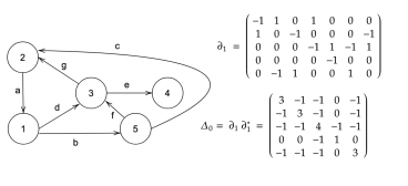
Figure 2: A graph considered as an arbitrarily oriented 1-complex and the corresponding boundary operator $\partial_{1}$ is shown. Notice that $\partial_{1}\partial_{1}^{*}$ is the traditional definition of the graph Laplacian. Here ^∗ represents matrix transpose.

Figure 1 illustrates our pipeline for an example design problem where the goal is to synthesize a material field for a solid rocket fuel, such that the burning fuel induces a prescribed thrust profile (thrust as a function of time). Such a problem exhibits the characteristics of where our approach is most applicable; the underlying domain $\Omega$ is largely fixed and the goal is to synthesize a material field over $\Omega$, and the analysis for the thrust may be provided by a custom numerical procedure. We will describe this problem and its solution in greater detail in Section 4. In general, for each design scenario, we assume that the design goals can be described through an objective, $f$ and a set of constraints, $g_{i}$ in the form of a general optimization problem:

$$\underset{\boldsymbol{\boldsymbol{w}}}{\text{min}} f(\boldsymbol{w})$$ (2)

s.t. $$g_{i}(\boldsymbol{w})\leq 0$$

where the optimization is coupled with a physical analysis. Note that our model reduction method is differentiable. Therefore, if the analytical gradients are already derived for the full material field, $\frac{\partial f}{\partial\boldsymbol{\mathcal{F}}}$, gradients for the reduced order problem can be computed through a simple chain rule multiplication

$$\frac{\partial f}{\partial\boldsymbol{w}}=\frac{\partial f}{\partial\boldsymbol{\mathcal{F}}}\frac{\partial\boldsymbol{\mathcal{F}}}{\partial\boldsymbol{w}}$$ (3)

where $\frac{\partial\boldsymbol{\mathcal{F}}}{\partial\boldsymbol{w}}$ is the constant reduced order basis matrix, $\boldsymbol{B}$.

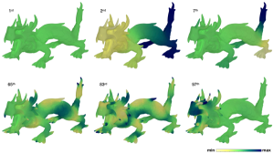
Figure 3: Spectral properties of Laplacian basis on an arbitrarily selected set. Notice the level of detail in the spatial field increases with the higher frequency basis functions.

3.2 Laplacian Eigenfunction Basis

The $i^{\mathrm{th}}$ combinatorial Laplacian operator over a finite oriented simplicial complex is defined as follows [37, 38, 39]

$$\Delta_{i}=\partial_{i+1}\partial_{i+1}^{*}+\partial_{i}^{*}\partial_{i}$$ (4)

Here $\partial_{i}$ represents the boundary operator for the $i^{\mathrm{th}}$ dimensional simplices, and $\partial_{i}^{*}$ is the adjoint operator of the boundary (aka the $i^{\mathrm{th}}$ co-boundary). The algebraic topological definition of the boundary operator on an oriented simplicial complex can be written as a matrix.

$$\partial_{i}=\begin{pmatrix}\iota_{1,1}&\iota_{1,2}&\cdots&\iota_{1,n}\\ \iota_{2,1}&\iota_{2,2}&\cdots&\iota_{2,n}\\ \vdots&\vdots&\ddots&\vdots\\ \iota_{m,1}&\iota_{m,2}&\cdots&\iota_{m,n}\end{pmatrix}$$ (5)

Here the oriented simplicial complex $\Omega$ has $m$ $i-1$ dimensional faces and $n$ $i$ dimensional faces; $\iota_{p,q}$ is $1$ if the $p^{\mathrm{th}}$ $i-1$ dimensional simplex is a positively oriented face of the $q^{\mathrm{th}}$ $i$ dimensional simplex, and $-1$ if the $i-1^{\mathrm{th}}$ dimensional simplex is negatively oriented. Considering finite simple graphs as (arbitrarily) oriented simplicial complexes of dimension 1, we notice that $\Delta_{0}$ is the graph Laplacian (since $\partial_{0}=0$). A simple example is shown in Figure 2. Note that when we have an oriented simplicial complex, the boundary is a linear operator written as a matrix multiplication. But the adjoint operator avoids the need to compute the boundary this way due to the duality with the graph Laplacian.

Considering a tetrahedral mesh $\Omega$ as an oriented simplicial complex of dimension 3 and computing $\Delta_{3}$ we obtain the definition $\Delta_{3}=\partial_{3}^{*}\partial_{3}$. Suppose we construct the dual complex $\bar{\Omega}$, where the $i$-simplices of the primal complex $\Omega$ are mapped to $3-i$ simplices in $\bar{\Omega}$. Then we observe the operator $\partial_{3}^{*}\partial_{3}$ over $\Omega$ is identical to $\partial_{1}\partial_{1}^{*}$ over $\bar{\Omega}$. Thus $\Delta_{3}$ over $\Omega$ is the graph Laplacian over $\bar{\Omega}$. Therefore we define the combinatorial Laplacian $\Delta_{3}=\boldsymbol{\mathcal{L}}=\boldsymbol{D}-\boldsymbol{A}$, where $\boldsymbol{D}$ is a diagonal matrix with each entry representing the element degree and $\boldsymbol{A}$ is the adjacency matrix given by

$$\boldsymbol{A}(i,j)=\begin{cases}1\text{ \; if elements i and j share a face,}\\ 0\text{ \; otherwise}\end{cases}$$ (6)

We also note that $\partial_{1}\partial_{1}^{*}$ is the (combinatorial) divergence of the gradient on the dual complex. The Laplacian eigenfunction bases are then derived by solving for the eigenvectors of $\boldsymbol{\mathcal{L}}$

$$\lambda_{i}\boldsymbol{e_{i}}=\boldsymbol{\mathcal{L}}\boldsymbol{e_{i}},\forall i$$ (7)

where $\lambda_{i}$ and $\boldsymbol{e_{i}}$ are the eigenvalues and eigenvectors of $\boldsymbol{\mathcal{L}}$, respectively. The basis matrix $\boldsymbol{B}$ can then be assembled by concatenating the eigenvectors side by side, $\boldsymbol{B}=[\boldsymbol{e_{1}},\boldsymbol{e_{2}},...,\boldsymbol{e_{k}}]\in\mathbb{R}^{n_{e}\times k}$, where $n_{e}$ represents the number of 3-simplices (tetrahedral elements). Using weights of the basis functions $\boldsymbol{w}=[w_{1},w_{2},...,w_{k}]^{T}$ as design variables, we represent the material field as $\boldsymbol{\mathcal{F}}=\boldsymbol{B}\boldsymbol{w}$. Although it is possible to compute all the available basis functions i.e.,  $k=n_{e}$, we avoid this costly operation in our sliding basis optimization by starting with a small number of functions $k\ll n_{e}$ and introduce additional eigenfunctions as needed by simply concatenating new basis vectors to the right side of the matrix B. To compute a small subset of eigenvectors in Eq. (7), we utilize the Spectra library [40] in our implementation.

Input: $n_{opt}$, $n_{s}$, $s_{max}$

Output: Optimized basis weights, $\boldsymbol{w}$

$i_{sb}\leftarrow 0$ $\triangleright$ Index for the first active basis set

$it_{s}\leftarrow 0$ $\triangleright$ Sliding iteration

$f\leftarrow 1/\epsilon$ $\triangleright$ A large number

$\boldsymbol{w}\leftarrow\varnothing$ $\triangleright$ Optimized basis weights

while not converged or $it_{s}<s_{max}$ do

       $\boldsymbol{w}_{s}$ $\leftarrow$ Initialize() $\triangleright$ Weights for active basis functions

       ($\boldsymbol{w}_{s}$, $f_{s}$) $\leftarrow$ Optimize($i_{sb}$, $n_{opt}$)

      

      if $f-f_{s}\geq\epsilon$ then

             $\boldsymbol{w}\leftarrow[\boldsymbol{w}[0:i_{sb}],~{}\boldsymbol{w}_{s}]$

             $f\leftarrow f_{s}$

             $it_{s}\leftarrow 0$

            

      else

             $\boldsymbol{w}\leftarrow[\boldsymbol{w},\boldsymbol{0}]$

             $it_{s}\leftarrow it_{s}+1$

            

       end if

      

      $i_{sb}\leftarrow i_{sb}+n_{s}$

      

end while

Algorithm 1 Sliding basis optimization

3.3 Optimization

We exploit the spectral property of the Laplacian basis (Figure 3) to explore the design space and iteratively optimize the material field. Figure 4 illustrates the basic idea of our sliding basis optimization. Here, $n_{opt}$ and $n_{s}$ are the number of active basis functions (i.e., optimization variables) and the amount of sliding at each sliding basis optimization step, respectively. We explore the basis space through multiple optimization operations where only the weights corresponding to the active $n_{opt}$ bases are optimized at a time. We optimize for only a small number of bases and we slide on the ordered basis axis by $n_{s}$ bases and perform another optimization with a new set of $n_{opt}$ variables. The sliding iterations continue until convergence.

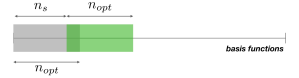
Figure 4: Sliding basis optimization starts by optimizing for the first $n_{opt}$ bases. Then, the selected basis are shifted by $n_{s}$ and the optimization is performed for the new set of $n_{opt}$ bases. This slide and optimize procedure continues until convergence.

Algorithm 1 describes the approach in detail. Given $n_{opt}$, $n_{s}$ and $s_{max}$ (the number of maximum trials before stopping if there is no significant improvement in objective value), the algorithm returns a set $\boldsymbol{w}$ of optimized basis weights. We choose $n_{s}<n_{opt}$ so that there is an overlapping set of active basis function whose weights are re-optimized (Figure 4) over the previous step. At each sliding basis optimization step, the weights $\boldsymbol{w}_{s}$ corresponding to the active basis functions (initially the first $n_{opt}$ eigenvectors of $\mathcal{L}$), are optimized to achieve the lowest possible objective value, $f_{s}$. Note that the optimization step here can be implemented using a commodity optimizer including a gradient based or a stochastic one. In our examples, we use sequential quadratic programming (SQP) [41] as it is an effective nonlinear programming method for general optimization problems. At each optimization step, we want to avoid getting stuck at the local minimum found in the previous step. This can happen, for example, if we initialize the weights for each new added basis to $0$ and use the previously optimized values for the weights of the overlapping basis functions. In contrast, initializing all the weights of an active basis set to be $0$ or random-valued perturbs the initial condition away from the previous local minumum. If the resulting optimized weights yield an objective value $f_{s}$ that is lower than $f$, the weights are accepted and $\boldsymbol{w}$ is expanded to include $\boldsymbol{w}_{s}$. If the objective value is not improved in the current iteration, the weights of the overlapping region are not modified and $\boldsymbol{w}$ is concatenated with $0$ weights corresponding to the newly added $n_{s}$ basis functions. Subsequently, the active set is modified by sliding towards the higher frequency basis functions. The sliding basis optimizations stops if the addition of the new basis does not significantly improve the objective or the maximum number of iterations are reached.

Suppose $k$ Laplacian basis functions are selected and a gradient based optimization approach such as SQP is utilized to solve a material design problem. The costliest step in such an approach is often the Hessian computation where the computational cost increases quadratically with the increasing number of design variables (i.e., number of basis functions in our case), $\mathcal{O}(k^{2})$. In cases involving black-box analysis of the objective (e.g. when the implementation for the physical simulation to evaluate the objective is unavailable), the conventional approach of optimizing all $k$ design variables at once results in $k^{2}$ analysis runs at each optimization step to construct the Hessian matrix. Given that analysis/ physical simulation is often expensive, the quadratic relationship makes the use of large $k$ impractical by creating computational bottlenecks. In the sliding basis optimization approach, the total computational cost is kept lower by exploring the same $k$ basis functions gradually, i.e. $n_{opt}$ functions at a time. In this case, only $n_{opt}^{2}$ analysis runs are required to construct the Hessian matrix. Here, it is important to note that $n_{opt}<<k$. As the optimizer needs to be reinitialized after each sliding iteration in our approach, $p=(k-n_{opt})/n_{s}+1$ complete optimization operations are performed to cover $k$ basis functions. Assuming same number of iterations are performed in each optimization operation and $n_{s}\rightarrow n_{opt}$, this translates to reducing the total computational cost by a factor of up to $n_{opt}/k$ over optimizing for fixed $k$ basis.

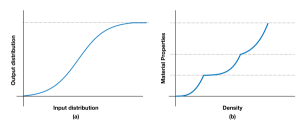
Figure 5: We utilize a gentle slope logistic function to bound the material distributions (a) and ordered SIMP approach to achieve discrete multi-material distribution (b).

For graded material design problems, bounds of the allowable material properties need to be enforced so that the optimized field can be manufactured. To enforce the bounds, one approach is to add additional linear inequality constraints in the form of $\boldsymbol{B}\boldsymbol{w}\leq u_{mb}$ and $\boldsymbol{B}\boldsymbol{w}\geq l_{mb}$ to the general optimization problem given in Eq. (2). However, this approach increases the number of constraint by 2*$n_{e}$ which could be in the order of hundred thousands for dense material distributions. This increase in the number of constraints slows down the optimization process significantly, especially for cases where the analytical gradients are not available. Instead, we use a filtering approach to bound the material distribution of the field without introducing additional constraints. We use a logistic function

$$l(x)=l_{mb}+\frac{u_{mb}-l_{mb}}{1+exp(-\kappa(x))}$$ (8)

where $\kappa$ is the steepness parameter set to give a gentle slope as shown in Figure 5.a. After the material field is computed as a weighted combination of the basis functions, we utilize the logistic function to enforce the bounds of the manufacturing technique. This approach provides a differentiable way to limit the material properties for manufacturability. Similarly, we enforce material constraints for multi-material optimization of discrete sets by combining this filtering approach with the penalization methods (Figure 5.b). We will now discuss these properties in the context of non-trivial design applications.

4 Applications

4.1 Graded Solid Rocket Fuel Design

In this application, our goal is to develop a computational tool to design a multi-material solid rocket propellant. Solid rocket propellant is shown at right with the inner surface geometry (where ignition takes place) in red and outer casing in blue.The propellant design should satisfy two main requirements: (1) The thrust generated as the propellant burns needs to match a given target thrust profile (2) No insulation should be required at the outer casing. The former requirement ensures that the rocket behaves as desired during its use. The latter requirement indicates that at the moment prior to burn out, all the casing surface is covered with some propellant material that will vanish at the same time, ensuring no part of the casing surface is exposed to on-going burning. Elimination of the insulation is an important innovation to substantially reduce the rocket weight. The time-varying nature of this problem brings up extra computational complexity in the analysis. Our model reduction and efficient sliding basis exploration plays a critical role for the solution of such a problem.

Physical Analysis

We first examine the physical relationships between a provided thrust profile (required thrust vs time) and the burn rate distribution of the rocket propellant and develop a boundary value problem to simulate the solid propellant burn. At any time $t$, the relationship between the thrust profile, $th(t)$ and the pressure inside the combustion chamber, $P_{c}(t)$ is given as

$$P_{c}\left(t\right)=\frac{th\left(t\right)}{C_{f}A_{t}},$$ (9)

where $C_{f}$ and $A_{t}$ are thrust coefficient and throat area, respectively. The mass flow rate of the exhaust gas emanating from the rocket nozzle is proportional to the pressure inside the chamber,

$$\dot{m}_{out}\left(t\right)=\frac{A_{t}P_{c}\left(t\right)}{c_{s}}.$$ (10)

Here $c_{s}$ represents the speed of sound. The mass flow rate emanating from the burn front can be calculated as a surface integral

$$\dot{m}_{in}\left(t\right)=\oiint_{\Gamma\left(t\right)}\rho_{p}\dot{r}\left(x,y,z\right)d\sigma,$$ (11)

where $\rho_{p}$ is the propellant density, $\dot{r}\left(x,y,z\right)$ is the spatial propellant burn rate distribution (as a function of the material at $(x,y,z)$) and $\Gamma\left(t\right)$ is the burn surface. The burn rate is related to the chamber pressure and the reference burn rate through the power law

$$\dot{r}\left(x,y,z\right)=\dot{r}_{ref}\left(x,y,z\right)\left(\frac{P_{c}}{P_{ref}}\right)^{n},$$ (12)

where $\dot{r}_{ref}\left(x,y,z\right)$ is the spatial distribution of the reference burn rate, $P_{ref}$ is the reference pressure and $n$ is the kinetic constant. Assuming a simplified mass conservation $\dot{m}_{in}\left(t\right)=\dot{m}_{out}\left(t\right)$, the thrust profile can be derived as a function of the reference burn rate:

$$th\left(t\right)=\left(P_{ref}^{-n}I_{sp}^{1-n}A_{t}^{-n}c_{s}^{n}\oiint_{\Gamma\left(t\right)}\rho_{p}\dot{r}_{ref}\left(x,y,z\right)d\sigma\right)^{\frac{1}{1-n}}$$ (13)

To close the Eq. 13, we model the evolution of the burn surface $\Gamma\left(t\right)$ using the Eikonal equation

$$\left|\nabla\phi\right|=\frac{1}{\dot{r}_{ref}\left(x,y,z\right)}.$$ (14)

The level sets of $\phi$ define the surface of the burn front at time instance $t$,

$$\Gamma(t)=\left\{\{x,y,z\}\in\mathbb{R}^{3}|\phi\left(x,y,z\right)=t\right\}.$$ (15)

We solve equations (13)-(15) assuming an axial symmetry inside a cylindrical rocket chamber with length, $L$ inner radius, $r_{in}$ and outer radius, $r_{out}$. When solving the boundary value problem we ensure the burn surface at the final time step is equal to the outer rocket case, $\Gamma_{case}$ i.e., $\Gamma\left(t_{end}\right)=\Gamma_{case}$.

Optimization Problem

We minimize the $\boldsymbol{\ell}^{2}$ norm of the error in matching the thrust profile while constraining the inner burn surface to avoid placing any insulating material

$$\underset{\boldsymbol{w}}{\text{min}} \sum_{t}(th(\boldsymbol{w})-th_{target})^{2}$$ (16)

s.t. $$r_{b}(\boldsymbol{w})^{i}>r_{in}$$

where $th_{target}$ and $th$ represent the target thrust profile and the current thrust profile achieved with the distribution $\boldsymbol{\mathcal{F}}=\dot{r}_{ref}(x,y,z)$ computed using the weights $\boldsymbol{w}$. Since the physical analysis solves a boundary value problem and constructs the level set of the burn surfaces starting from the outer case, we are able to optimize the material distribution such that the initial burn surface comes as a byproduct. For each material distribution, we represent the inner burn surface through a set of radius values, $r_{b}^{i}$, and check if they are all inside the allowable inner surface region defined by the radius value, $r_{in}$.

4.2 Multi-Material Topology Optimization

We apply our sliding basis optimization approach to the design of multi-material distributions with given discrete set of predefined materials for structural mechanics problems.

Physical Analysis

Assuming linear isotropic materials and small deformations, we solve the linear elasticity problem $\boldsymbol{K}\boldsymbol{u}=\boldsymbol{F}$ where $\boldsymbol{K}$, $\boldsymbol{u}$ and $\boldsymbol{F}$ are the stiffness matrix, nodal displacement vector, and nodal external force vector, respectively. In our implementation, we discretize the domain using tetrahedral elements characterized by linear shape functions assuming static load and fixed displacement boundary conditions.

Table 1: Performance of our sliding basis optimization algorithm for the graded solid rocket design problem on a variety of target thrust profiles. Performance of fixed basis reduced order optimization is also provided for comparison. Note that fixed basis optimization and sliding basis optimization cover the same basis functions.

					Fixed Basis		Sliding Basis
Thrust Profile	$n_{opt}$	$n_{s}$	$n_{slides}$	Total Basis	Time	Objective/Error	Time	Objective/Error
Constant Acceleration	20	15	14	230	1178s	349k/2.3%	288s	86k/1.1%
Constant Deceleration	50	40	7	320	4896s	867k/3.4%	621s	452k/2.7%
Two Step	20	15	7	125	191s	102k/1.1%	69s	217k/1.4%
Bucket	20	15	24	380	1006s	272k/1.8%	596s	272k/1.8%

Optimization Problem

We formulate the multi-material design optimization as a density based topology optimization problem with compliance minimization and mass fraction constraint as

$$\underset{\boldsymbol{w}}{\text{min}} \boldsymbol{u}^{T}\boldsymbol{K(\boldsymbol{w})}\boldsymbol{u}$$ (17)

s.t. $$m(\boldsymbol{w})/m_{0}\leq m_{frac}$$

$$\boldsymbol{K(\boldsymbol{w})}\boldsymbol{u}=\boldsymbol{F}$$

where $m$, $m_{0}$ and $m_{frac}$ are mass of the current design, mass of the design domain fully filled with maximum density and prescribed mass fraction. Here, $\boldsymbol{u}^{T}\boldsymbol{K}\boldsymbol{u}$ represents the compliance of the structure. We adopt the ordered multi-material SIMP interpolation approach [9] since it does not introduce additional variables and computational complexity as the number of materials increase. We incorporate the interpolation step after computing the density field with the weights and basis functions and using the bounding filter to keep density values in $[0,1]$ limits as explained in Section 3.3. Additionally, we implemented the density filtering approach described in [42]. This filter is often utilized to avoid checkerboard issues in traditional topology optimization. We observe similar issues as we use higher order basis functions although we use a reduced order approach. We found the density filtering helpful in avoiding those issues in our reduced order approach as well.

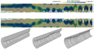
Figure 6: Top image shows the progression of the burn front (black lines) on the cross section of solid rocket with the graded burn rate distribution for the constant acceleration thrust profile. The arrows on the right denote the burn direction. Notice the lines spread apart in high burn rate material regions (blue) compared to the low burn rate regions(yellow) indicating faster burn. Bottom three cutouts show the solid rocket fuel at three stages of the burn propagation.

5 Results and Discussions

We demonstrate the results of using sliding basis optimization in the applications described in Section 4. We discuss the progression of the optimization during sliding steps, performance gain and effect of sliding amount.

Graded solid rocket fuel design

The sliding basis optimization results for four different thrust profiles (constant acceleration, constant deceleration, two step and bucket) are presented in Fig. 7. Since our physical analysis assumes axially symmetric material distributions, we parameterize the cross section and compute the basis functions on it. We treat the analysis (solving the boundary value problem described in Section 4) as a black-box solver and do not derive the analytical gradients for this application to show the effectiveness of our sliding basis optimization approach. As shown in Fig. 6, we parameterize the burn rate distribution on the whole rectangular cross section. For all of our examples, we used 3000 quad elements on the cross section. Due to the boundary value problem formulation which takes the last burn front (outer cylindrical surface) as input, the inner burn surface is computed as a byproduct of the simulation. After the optimization is completed, we mask out the portions of the cross section that are beyond the inner surface since these portions are not needed to achieve the desired target thrust profile behavior.

One challenge in matching the thrust profiles is to be able to reduce the thrust significantly through the end of the burn process (e.g., constant deceleration profile). At a given time, the thrust is proportional to the area of the burn front surface. Since the surface area naturally increases as the burn surface propagates from inside to the outside of the cylinder, reducing thrust requires complex material distributions that can reverse this natural tendency to increase burn surface area. Therefore, the constant deceleration profile is more challenging and requires more complex material distributions than the constant acceleration profile. Table 1 reports the parameters used in our examples and performance of our sliding basis optimization through time, objective value and the average percentage error between the target and optimized thrust profiles. While we use 20 optimization variables, $n_{opt}$ for the constant acceleration, two step and bucket profiles, we observe that using 50 optimization variables results in better performance for constant deceleration profile. We believe this is mainly due to the challenging nature of this profile that requires more complex distributions that can be achieved using more basis functions.

Figure 8 shows the target and optimized thrust profile results during six steps of sliding basis optimization for two step thrust profile. The first optimization step that uses only twenty basis functions does not match the target profile well since the small number of basis functions is not enough to create complex enough material distributions for this case. In the consecutive steps, however, the resulting thrust profiles progressively match the target better as more basis functions are incorporated with each slide. Finally, the sliding optimization stops when the convergence criteria is satisfied. For this application, we used 5% error in the profile match as the convergence criteria.

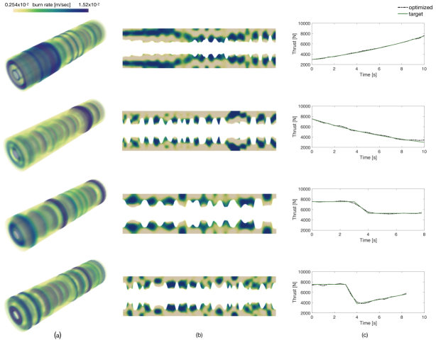
Figure 7: Solid rocket fuel design results with volume render of the burn rate distribution (a), cross section of the rocket geometry with inner surface (b) and thrust profile plot (c). The images and plots from top to bottom represent the results of constant acceleration, constant deceleration, two step and bucket profiles.

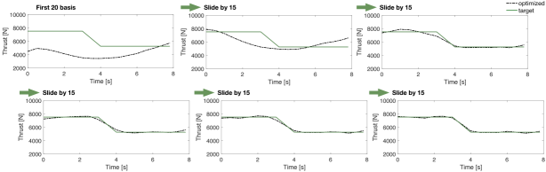
Figure 8: Progression of thrust profile match through the sliding basis optimization. With only first few basis functions, the results may be far from the desired. However, the optimizer recovers from those results with the additional sliding optimization steps since more basis functions are used.

We compare the sliding basis optimization to the reduced order approach using a predetermined number of Laplacian basis functions during the optimization such that all basis functions are optimized simultaneously. Note that this ‘fixed basis’ approach is already a reduced order method and significantly improves optimization performance by projecting optimization variables into lower dimensional space. Table 1 reports the performance of both fixed and sliding basis optimization methods. Our sliding basis approach can speed up the optimization process up to 8 times over the fixed basis method while exploring the same number of basis functions. In addition to the time gain, sliding basis optimization results in better objective minimization performance in most of our examples. We believe this may be due to the random initialization at each sliding step that acts as local perturbations and alleviate local minima issues of general nonlinear optimization problems. All computations are performed and recorded on a computer with 16GB memory and 3.1GHz i7 processor.

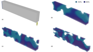
Figure 9: Multi-material topology optimization results for the cantilever beam problem throughout the sliding steps. (a) problem setup with boundary conditions (blue regions) and external loads (yellow arrows). (b)-(d): optimized material distributions for two materials and void.

Multi-material topology optimization

Figure 9 presents the problem setup (a) and the optimized material distributions for three steps of the sliding basis optimization (b-d) for the cantilever beam. For this beam example, we use a discrete set of void and two materials with normalized density values of $0,~{}0.1$ and $1$ and Young’s modulus values of $0,~{}2GPa$ and $3GPa$. From Figure 9(b) to Figure 9(d), number of optimized basis functions increase from 20 to 170 indicating the complexity of material distribution increases as the number of basis functions increases. This sliding basis optimization is performed using $n_{opt}=20$ and $n_{s}=15$ with mass fraction constraint, $m_{frac}$ of 0.5 on a mesh with 19567 tetrahedral elements. Using numerical gradients (i.e., treating simulation as black-box), we observe that sliding basis optimization results in approximately 3 times faster computation time ($87mins$ vs $259mins$) compared to fixed basis optimization with 170 basis.

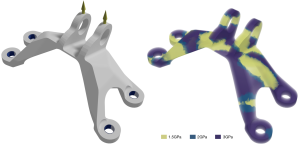
Figure 10: Multi-material topology optimization result for the bracket model. Left: problem setup with boundary conditions (blue regions) and external loads (yellow arrows). Right: optimized material distribution is given for three material set.

The optimized material distribution of the bracket model is given in Figure 10 for a discrete set with three materials (normalized densities: $0.1,~{}0.3,~{}1$ and Young’s modulus: $1.5GPa,~{}2.5GPa,~{}3GPa$). It can be observed that the optimizer places the strongest material on the load paths an around the high stress regions such as where the boundary conditions and forces are applied. The optimization is performed using $n_{opt}=20$ and $n_{s}=15$ with mass fraction constraint, $m_{frac}$ of 0.5 on a mesh with 174454 tetrahedral elements. For this particular example, instead of using the numerical gradients, we derived and utilized the analytical gradients. The analytical gradient computation is an extremely fast operation for compliance minimization. Thus, the only costly operation during the optimization is the linear solve while finding the Lagrange multipliers. However, the computational cost of a linear solve operation with a matrix of size 20 or 200 are marginally different for state of the art linear solvers. Therefore, we do not observe a computational gain for using the sliding basis optimization over the fixed basis optimization for this particular compliance minimization problem when analytical gradients are utilized. However, note that fixed basis optimization already reduces the computational cost of the linear solve from a matrix of size 174454 to a matrix of 200. Furthermore, sliding basis optimization could provide more significant computational gain over fixed basis for problems with costly analytical gradient computations.

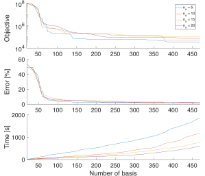
Figure 11: Effect of sliding amount to convergence with objective value (shown in log scale), target profile matching error and computation time.

Figure 11 demonstrates convergence of our optimization with respect to number of explored basis functions for different sliding amount values, $n_{s}$. We provide objective value in log scale, the average percentage error in target profile matching and computation time. In terms of selecting the sliding amount, we found that lowering the sliding amount and re-optimizing for more basis functions might give better objective reduction capabilities for lower number of explored basis functions. However, as the number of explored basis increases, all $n_{s}$ values converge to similar objective values. Additionally, small sliding amounts take more computational time to cover the same amount of basis functions since more basis functions are re-optimized due to the overlap. In summary, we found that using large sliding amounts ($n_{s}~{}n_{opt}$) with small overlap works well resulting in similar objective minimization performance compared to small sliding amounts with minor increase in computational time. In our examples, we observed that $n_{s}\approx 0.75*n_{opt}$ gives a good trade off between objective minimization and computational performance.

We compare our Laplacian basis formulation to classical topology optimization like conventional approach where value of element is optimized independently in Figure 12. It can be observed that the results of the Laplacian basis are smoother since low number of basis functions are used and they correspond to lower frequency basis functions. We can see that there is less than 0.3% objective value difference between the conventional approach and the sliding basis optimized result while the difference between the optimization time is significant. For this example, we run the solid rocket fuel design problem for the two-step thrust profile. Note that we have reduced grid resolution to 1800 to be able to run the conventional approach in practical times. As we increase the resolution and thus number of optimization variables, computational time gain increases.

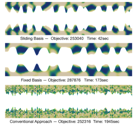
Figure 12: Comparison of objective value and computation time for sliding basis optimization, fixed basis optimization and conventional optimization approach.

Limitations

Since our formulation is a reduced order approach, the solution space is limited by the basis functions used during the optimization. Thus, there may be a better optimum that lies outside this space that cannot be reached by using a small number of basis functions ($k\sim 100$) compared to optimizing for all elements of the mesh domain ($n_{e}\sim 100k$). However, our examples demonstrate that the small number of basis functions are capable of satisfying the design requirements and enable solution of otherwise intractable computationally demanding problems.

We apply our sliding basis optimization to general nonlinear optimization problems. Unfortunately, finding the global optimum of such problems is still an open problem and our approach does not guarantee that the optimized solutions are globally optimum. Similar to traditional topology optimization approaches, different initial conditions may give different locally optimum results. Depending on the problem, this may be an important challenge. However, for compliance minimization, we do not observe significantly different results for different initial conditions in terms of the minimized compliance value. Moreover, our re-initialization at each step of the sliding optimization and re-optimization of overlapping basis functions help alleviate these local minima issues.

6 Conclusion and Future Work

Given a design domain and a set of goals in the form of objective and constraints, we present a method to design multi-material distributions. To solve the material distribution design problem with a reduced order approach, we use Laplacian eigenfunctions as a basis and project the design space into lower dimensions with fixed number of basis functions. Further, we extend this fixed basis optimization approach to a sliding basis method where the key idea is to exploit the spectral properties of the Laplacian basis for efficient exploration in the reduced space. Our sliding basis approach provides a flexible and powerful mechanism enabling computationally demanding design optimization problems involving black-box analysis. In this work, we show its efficiency on two applications as graded solid rocket fuel design and multi-material topology optimization. When tested with black-box analysis, our sliding basis approach can speed up the optimization process up to 8 times over the fixed basis method, often leading to better objective minimization due to local perturbations at each sliding step. We believe the ability to work with black-box analysis is very important for facilitating innovation and promoting engineering collaboration.

In this work, we focus on design material distribution fields. However, our approach generalizes to any spatial field design such as displacement fields. In future, other basis functions exhibiting similar spectral properties can be explored and incorporated into our sliding basis optimization method. Musialski et al.  [43] presents a reduced order method for surface design. Complementing our approach with a such parametrization could allow efficient design of surface geometries increasing surface detail in a sliding manner similar to increasing the detail in material distribution.

7 Acknowledgments

The authors would like to thank NASA Jacobs Space Exploration Group for providing the solid rocket fuel design problem with the target thrust profile. This research was developed with funding from the Defense Advanced Research Projects Agency (DARPA). The views, opinions and/or findings expressed are those of the authors and should not be interpreted as representing the official views or policies of the Department of Defense or U.S. Government. 3D models: dragon by XYZ RGB Inc and GE bracket by WilsonWong on GrabCAD.

References

References

- [1] Stratasys Connex Objet, https://www.stratasys.com/3d-printers/objet-350-500-connex3, accessed: 2019-08-07.
- [2] Insstek DMT, http://www.insstek.com/content/multi_materials, accessed: 2019-08-07.
- [3] L. Li, J. Wang, P. Lin, H. Liu, Microstructure and mechanical properties of functionally graded ticp/ti6al4v composite fabricated by laser melting deposition, Ceramics International 43 (18) (2017) 16638 – 16651. doi:https://doi.org/10.1016/j.ceramint.2017.09.054.
- [4] A. Bandyopadhyay, B. Heer, Additive manufacturing of multi-material structures, Materials Science and Engineering: R: Reports 129 (2018) 1 – 16. doi:https://doi.org/10.1016/j.mser.2018.04.001.
- [5] M. P. Bendsøe, O. Sigmund, Topology Optimization: Theory, Methods and Applications, Springer, 2004.
- [6] L. Davis, Handbook of genetic algorithms.
- [7] S. Kirkpatrick, C. D. Gelatt, M. P. Vecchi, Optimization by simulated annealing, science 220 (4598) (1983) 671–680.
- [8] O. Sorkine, Laplacian mesh processing, in: Eurographics (STARs), 2005, pp. 53–70.
- [9] W. Zuo, K. Saitou, Multi-material topology optimization using ordered simp interpolation, Structural and Multidisciplinary Optimization 55 (2) (2017) 477–491.
- [10] J. P. Blasques, Multi-material topology optimization of laminated composite beams with eigenfrequency constraints, Composite Structures 111 (2014) 45–55.
- [11] M. Y. Wang, X. Wang, “color” level sets: a multi-phase method for structural topology optimization with multiple materials, Computer Methods in Applied Mechanics and Engineering 193 (6-8) (2004) 469–496.
- [12] A. M. Mirzendehdel, K. Suresh, A pareto-optimal approach to multimaterial topology optimization, Journal of Mechanical Design 137 (10) (2015) 101701.
- [13] C. Conlan-Smith, K. A. James, A stress-based topology optimization method for heterogeneous structures, Structural and Multidisciplinary Optimization 60 (1) (2019) 167–183.
- [14] P. Vogiatzis, S. Chen, X. Wang, T. Li, L. Wang, Topology optimization of multi-material negative poisson’s ratio metamaterials using a reconciled level set method, Computer-Aided Design 83 (2017) 15–32.
- [15] B. Vaissier, J.-P. Pernot, L. Chougrani, P. Véron, Parametric design of graded truss lattice structures for enhanced thermal dissipation, Computer-Aided Design 115 (2019) 1–12.
- [16] D. Li, W. Liao, N. Dai, G. Dong, Y. Tang, Y. M. Xie, Optimal design and modeling of gyroid-based functionally graded cellular structures for additive manufacturing, Computer-Aided Design 104 (2018) 87–99.
- [17] Y. Choi, G. Oxberry, D. White, T. Kirchdoerfer, Accelerating topology optimization using reduced order models, Tech. rep., Lawrence Livermore National Lab.(LLNL), Livermore, CA (United States) (2019).
- [18] D. Amsallem, M. J. Zahr, Y. Choi, C. Farhat, Design optimization using hyper-reduced-order models, Structural and Multidisciplinary Optimization 51 (2015) 919–940.
- [19] C. Gogu, Improving the efficiency of large scale topology optimization through on-the-fly reduced order model construction, International Journal for Numerical Methods in Engineering 101 (4) (2015) 281–304.
- [20] G. H. Yoon, Structural topology optimization for frequency response problem using model reduction schemes, Computer Methods in Applied Mechanics and Engineering 199 (25-28) (2010) 1744–1763.
- [21] J. K. Guest, L. C. Smith Genut, Reducing dimensionality in topology optimization using adaptive design variable fields, International journal for numerical methods in engineering 81 (8) (2010) 1019–1045.
- [22] T. A. Poulsen, Topology optimization in wavelet space, International Journal for Numerical Methods in Engineering 53 (3) (2002) 567–582.
- [23] P. Zhou, J. Du, Z. Lü, Highly efficient density-based topology optimization using dct-based digital image compression, Structural and Multidisciplinary Optimization 57 (1) (2018) 463–467.
- [24] D. A. White, M. L. Stowell, D. A. Tortorelli, Toplogical optimization of structures using fourier representations, Structural and Multidisciplinary Optimization 58 (3) (2018) 1205–1220.
- [25] N. G. Ulu, S. Coros, L. B. Kara, Designing coupling behaviors using compliant shape optimization, Computer-Aided Design 101 (2018) 57–71.
- [26] E. Ulu, J. Mccann, L. B. Kara, Lightweight structure design under force location uncertainty, ACM Transactions on Graphics (TOG) 36 (4) (2017) 158.
- [27] B. Levy, Laplace-beltrami eigenfunctions towards an algorithm that” understands” geometry, in: IEEE International Conference on Shape Modeling and Applications 2006 (SMI’06), IEEE, 2006, pp. 13–13.
- [28] B. Lévy, S. Petitjean, N. Ray, J. Maillot, Least squares conformal maps for automatic texture atlas generation, in: ACM transactions on graphics (TOG), Vol. 21, ACM, 2002, pp. 362–371.
- [29] B. Vallet, B. Lévy, Spectral geometry processing with manifold harmonics, in: Computer Graphics Forum, Vol. 27, Wiley Online Library, 2008, pp. 251–260.
- [30] R. Liu, H. Zhang, Segmentation of 3d meshes through spectral clustering, in: 12th Pacific Conference on Computer Graphics and Applications, 2004. PG 2004. Proceedings., IEEE, 2004, pp. 298–305.
- [31] O. Sorkine, D. Cohen-Or, Y. Lipman, M. Alexa, C. Rössl, H.-P. Seidel, Laplacian surface editing, in: Proceedings of the 2004 Eurographics/ACM SIGGRAPH symposium on Geometry processing, ACM, 2004, pp. 175–184.
- [32] H. Xu, Y. Li, Y. Chen, J. Barbič, Interactive material design using model reduction, ACM Transactions on Graphics (TOG) 34 (2) (2015) 18.
- [33] H. Zhang, Discrete combinatorial laplacian operators for digital geometry processing, in: Proceedings of SIAM Conference on Geometric Design and Computing. Nashboro Press, 2004, pp. 575–592.
- [34] B. Lévy, H. R. Zhang, Spectral mesh processing, in: ACM SIGGRAPH 2010 Courses, SIGGRAPH ’10, ACM, New York, NY, USA, 2010, pp. 8:1–8:312. doi:10.1145/1837101.1837109.
- [35] R. Song, L. Wang, Multiscale representation of 3d surfaces via stochastic mesh laplacian, Computer-Aided Design 115 (2019) 98–110.
- [36] G. Taubin, A signal processing approach to fair surface design, in: Proceedings of the 22nd annual conference on Computer graphics and interactive techniques, ACM, 1995, pp. 351–358.
- [37] D. Horak, J. Jost, Spectra of combinatorial laplace operators on simplicial complexes, Advances in Mathematics 244 (2013) 303–336.
- [38] T. E. Goldberg, Combinatorial laplacians of simplicial complexes, Senior Thesis, Bard College.
- [39] A. Duval, V. Reiner, Shifted simplicial complexes are laplacian integral, Transactions of the American Mathematical Society 354 (11) (2002) 4313–4344.
- [40] Y. Qiu, SpectrA: Sparse Eigenvalue Computation Toolkit as a Redesigned ARPACK, https://spectralib.org/ (2015–2019).
- [41] J. Nocedal, S. J. Wright, Numerical Optimization, Second Edition, Springer, 2006.
- [42] E. Andreassen, A. Clausen, M. Schevenels, B. S. Lazarov, O. Sigmund, Efficient topology optimization in matlab using 88 lines of code, Structural and Multidisciplinary Optimization 43 (1) (2011) 1–16.
- [43] P. Musialski, T. Auzinger, M. Birsak, M. Wimmer, L. Kobbelt, Reduced-order shape optimization using offset surfaces., ACM Trans. Graph. 34 (4) (2015) 102–1.