Uncertainty quantification in first-principles predictions of phonon properties and lattice thermal conductivity

Abstract

We present a framework for quantifying the uncertainty that results from the choice of exchange-correlation (XC) functional in predictions of phonon properties and thermal conductivity that use density functional theory (DFT) to calculate the atomic force constants. The energy ensemble capabilities of the BEEF-vdW XC functional are first applied to determine an ensemble of interatomic force constants, which are then used as inputs to lattice dynamics calculations and a solution of the Boltzmann transport equation. The framework is applied to isotopically-pure silicon. We find that the uncertainty estimates bound property predictions (e.g., phonon dispersions, specific heat, thermal conductivity) from other XC functionals and experiments. We distinguish between properties that are correlated with the predicted thermal conductivity [e.g., the transverse acoustic branch sound speed ($R^{2}=0.89$) and average Grüneisen parameter ($R^{2}=0.85$)] and those that are not [e.g., longitudinal acoustic branch sound speed ($R^{2}=0.23$) and specific heat ($R^{2}=0.00$)]. We find that differences in ensemble predictions of thermal conductivity are correlated with the behavior of phonons with mean free paths between $100$ and $300$ nm. The framework systematically accounts for XC uncertainty in phonon calculations and should be used whenever it is suspected that the choice of XC functional is influencing physical interpretations.

I Introduction

Ab initio predictions of the lattice thermal conductivity of crystalline materials have become increasingly widespread due to their accuracy when compared to experimental measurements.Broido et al. (2007); McGaughey et al. (2019); Lindsay et al. (2018) The prediction framework relies on density functional theory (DFT) to determine interatomic force constants, which quantify the change in potential energy of a material when its atoms are displaced from their equilibrium positions. The force constants are then used to predict harmonic phonon properties such as dispersion relations, group velocities, specific heat, and, by solving the phonon Boltzmann transport equation (BTE), anharmonic properties like scattering rates. McGaughey et al. (2019) These properties are then used to predict the thermal conductivity. This approach has been successful in studies of both low and high thermal conductivity materials, Lindsay et al. (2013); Shiga et al. (2012); Ward et al. (2009); Feng et al. (2015a); Li et al. (2012); Broido et al. (2007) and the predictions can be performed using one of several open-source packages. Tadano et al. (2014); Carrete et al. (2017); Togo et al. (2015); Li et al. (2014) Models have grown more sophisticated in recent years to capture increasingly complex phenomena and resolve discrepancies between predictions and experimental values. Lindsay et al. (2019) For example, while it is common practice to consider only three-phonon scattering processes in solving the BTE, recent work has shown that four-phonon scattering is strong enough to reduce the predicted thermal conductivity in a range of materials. Yang et al. (2019); Feng and Ruan (2018); Feng et al. (2017); Tian et al. (2018); Ravichandran and Broido (2018) There has also been progress in the treatment of finite temperature phases, Shulumba et al. (2017a, b); Souvatzis et al. (2009); Tadano and Tsuneyuki (2015) compositionally-disordered materials, Garg et al. (2011); Wang et al. (2011); Eliassen et al. (2017); Arrigoni et al. (2018) and defects. Feng et al. (2015b); Wang et al. (2017); Guo and Lee (2020)

While the continued improvement of models is important, the quality of the predictions also depends on computational parameters. McGaughey et al. (2019); Jain and McGaughey (2015); Xie et al. (2017) Obtaining converged phonon lifetimes, for example, requires a sufficiently-large cutoff radius for anharmonic interactions and a sufficiently-dense phonon wave vector grid. Similarly, the quality of the required force constants depends on the quality of the DFT calculation, which in turn is affected by a variety of factors. Some of these factors, such as the electronic wave vector grid and the plane wave energy cutoff (if a plane wave basis is used), require convergence testing. The exchange-correlation (XC) functional, conversely, is a critical component of all DFT calculations that must simply be chosen, sometimes with no a priori knowledge of the most suitable selection.

The impact of XC functional choice, which we call the XC uncertainty, can be examined by changing the XC functional in otherwise identical thermal conductivity calculations. Jain and McGaughey calculated the thermal conductivity of silicon at a temperature of 300 K using five different XC functionals. Jain and McGaughey (2015) They showed that the predictions could be as low as 127 W/m-K or as high as 172 W/m-K, in comparison with the experimental value of 153 W/m-K. Inyushkin et al. (2004) They argued that the variation was a result of differences in predictions of group velocities, three-phonon scattering phase space, and anharmonic effects. Taheri et al. calculated the thermal conductivity of graphene using three XC functionals and found the predictions to range from 5400 to 8700 W/m-K at a temperature of 300 K. Taheri et al. (2018) Qin et al. also performed calculations on graphene at the same temperature using eight different XC functionals and reported a thermal conductivity range of 1900 to 4400 W/m-K. Qin et al. (2018) In contrast to the silicon study by Jain and McGaughey, both Taheri et al. and Qin et al. found that all XC functionals tested agreed in predicting harmonic properties such as group velocity and three-phonon phase space, implying that the anharmonic properties are responsible for the large range of predicted thermal conductivities in graphene. These three previous studies demonstrate the impact of XC functional choice in predicting thermal conductivity, but the results are not conclusive indicators of XC uncertainty because the XC functionals tested were somewhat arbitrary. Additionally, this approach is computationally inefficient because nearly identical calculations must be performed for each XC functional choice. Given the large number of possible functionals, even within the generalized gradient approximation (GGA) space, this brute force approach becomes computationally infeasible.

The Bayesian error estimation functional with van der Waals (BEEF-vdW) correlation is an XC functional that can systematically estimate XC uncertainty in DFT energies. Wellendorff et al. (2012) It possesses built-in uncertainty estimation capabilities in the form of an ensemble of GGA XC functionals that are calibrated to reproduce the discrepancies observed between experimental measurements and DFT predictions. The estimate obtained from the BEEF-vdW ensemble is computationally efficient because results for thousands of XC functionals are obtained non-self-consistently through a single self-consistent calculation. BEEF-vdW has been applied to quantify XC uncertainty in predictions of molecular vibrational frequencies, Parks et al. (2019) magnetic ground states, Houchins and Viswanathan (2017), intercalation energies, Pande and Viswanathan (2018) heterogeneous catalysis, Medford et al. (2014); Krishnamurthy et al. (2019); Christensen et al. (2015a) electrocatalysis, Deshpande et al. (2016); Krishnamurthy et al. (2018); Christensen et al. (2015b) mechanical properties of solid electrolytes, Ahmad and Viswanathan (2016) and thermodynamic properties. Guan et al. (2019) Such uncertainty estimates are useful in machine learning-based materials design applications. For example, knowing the uncertainty associated with a DFT calculation can improve the robustness of workflows that rely on ab initio calculations to screen materials. Ramprasad et al. (2017); Ulissi et al. (2017)

In this work, we present a framework to estimate the XC uncertainty in predictions of phonon properties, specific heat, and thermal conductivity. The calculation details are presented in Sec. II. While we include only three-phonon scattering to save on computational cost, the framework can be easily extended to account for four-phonon and other scattering mechanisms. The framework is then applied in Sec. III to isotopically-pure silicon, which is chosen due to its popularity as a benchmark for thermal conductivity predictions. McGaughey et al. (2019); Jain and McGaughey (2015); Esfarjani et al. (2011); Broido et al. (2007) For comparison to the BEEF-vdW ensemble results, predictions of phonon properties, specific heat, and thermal conductivity using the LDA, Perdew and Wang (1992) PBE, Perdew et al. (1996) PBEsol, Perdew et al. (2008) and optPBE-vdW Klimeš et al. (2009) XC functionals are also presented. We find that the BEEF-vdW ensemble accurately describes the variation of the self-consistent DFT predictions, with most predicted quantities bounded to within two ensemble standard deviations of the BEEF-vdW predictions. Based on analysis of the BEEF-vdW ensemble, we find that the best predictors of silicon thermal conductivity are the transverse acoustic phonon sound speed and $\mathbf{X}$-point frequency and the average Grüneisen parameter. We also demonstrate the sensitivity of the thermal conductivity prediction to contributions of phonons with mean free paths in the range of $100$ to 300 nm.

II Methods

II.1 Bayesian error estimation

BEEF-vdW is a semi-empirical XC functional that provides a way to systematically estimate the XC uncertainty in a DFT calculation. Its model space for the exchange-correlation energy $E_{\text{XC}}$ is given by Wellendorff et al. (2012)

$$E_{\text{XC}}=\sum_{m=0}^{29}\left(a_{m}E_{m}^{\text{GGA-x}}\right)+\alpha_{c}E^{\text{LDA-c}}+(1-\alpha_{c})E^{\text{PBE-c}}+E^{\text{nl-c}}.$$ (1)

Here, $E^{\text{LDA-c}}$, $E^{\text{PBE-c}}$, and $E^{\text{nl-c}}$ are the correlation contributions from the local Perdew-Wang LDA correlation, Perdew and Wang (1992) the semi-local Perdew-Burke-Ernzerhof (PBE) correlation, Perdew et al. (1996) and the vdW-DF2 nonlocal correlation. Lee et al. (2010) $E_{m}^{\text{GGA-x}}$ is the contribution to the exchange energy and is given by

$$E_{m}^{\text{GGA-x}}=\int\epsilon_{\text{x}}^{\text{UEG}}[n(\mathbf{r})]B_{m}\{t[n(\mathbf{r}),\nabla n(\mathbf{r})]\}d\mathbf{r},$$ (2)

where $n(\mathbf{r})$ and $\nabla n(\mathbf{r})$ are the electron density and its gradient, $t$ is a function taking $n(\mathbf{r})$ and $\nabla n(\mathbf{r})$ as its inputs, $\epsilon_{\text{x}}^{\text{UEG}}$ is the exchange energy density of the uniform electron gas, and $B_{m}$ is the $m$th Legendre polynomial.

Wellendorff et al. fit the parameters $a_{m}$ ($0\leq m\leq 29$) and $\alpha_{c}$ to experimental training data to determine the optimal, or “best-fit,” BEEF-vdW XC functional. Wellendorff et al. (2012) The training data included six different data sets consisting of molecular formation and reaction energies, molecular reaction barriers, non-covalent interactions, solid-state properties such as cohesive energies and lattice constants, and chemisorption energies on solid surfaces. The training data did not include vibrational frequencies or thermal conductivities, so that our work will also serve as a test of the transferability of BEEF-vdW for predicting these properties.

BEEF-vdW provides a systematic and computationally-efficient approach to estimate the XC uncertainty in a DFT energy calculation through an ensemble of XC functionals. The electron density is first obtained through a self-consistent DFT calculation using the best-fit functional. An ensemble of XC functionals, each of which has its own set of $a_{m}$ and $\alpha_{c}$, are then applied to that electron density to yield an ensemble of non-self-consistent XC energies using Eq. (1). Wellendorff et al. generated the ensemble of XC functionals using the following method. For every batch of data in the training set:

1. Use the best-fit XC functional to predict the values of interest and compare them with the experimental values. Call the sample standard deviation of these differences $s_{1}$.

2. Use the XC functional ensemble to predict the values of interest. Call the sample standard deviation of the ensemble $s_{2}$.

By tuning the distributions of $a_{m}$ and $\alpha_{c}$, Wellendorff et al. set $s_{1}$ and $s_{2}$ to be approximately equal, so that the spread in the ensemble recreates the differences between the experimental data and the best-fit BEEF-vdW predictions.

While the BEEF-vdW XC functional ensemble was generated to recreate differences between experimental and DFT data, there is no guarantee of its suitability for predicting properties not considered in the original training data set. The results of subsequent studies, Houchins and Viswanathan (2017); Ahmad and Viswanathan (2016); Parks et al. (2019); Medford et al. (2014); Krishnamurthy et al. (2019); Christensen et al. (2015a); Deshpande et al. (2016); Krishnamurthy et al. (2018); Christensen et al. (2015b); Guan et al. (2019) however, demonstrated that the ensemble can reliably describe the XC uncertainty in self-consistent DFT predictions of a wide range of systems and material properties. In other words, the ensemble is transferable, in the sense that the variation in most self-consistent predictions is bounded in an interval of a few ensemble standard deviations. This result likely emerges because the ensemble exchange enhancement factors are similar to other common GGA-level functionals for reduced density gradient ($s=|\nabla n|/2k_{\text{F}}n$, where $k_{\text{F}}$ is the Fermi wave vector for a uniform electron gas) values between 0 and 2, Wellendorff et al. (2012) a range that describes most important interactions in chemical and solid-state systems. Wellendorff et al. (2012); Hammer et al. (1999); Csonka et al. (2009)

II.2 Phonon properties and lattice thermal conductivity

II.2.1 Lattice thermal conductivity

The phonon contribution to the thermal conductivity of a crystalline solid, i.e., the lattice thermal conductivity in direction $l$, $k_{l}$, can be obtained by solving the BTE in combination with the Fourier law and is given by McGaughey et al. (2019)

$$k_{l}=\sum_{\mathbf{q},\nu}c(\mathbf{q},\nu)v_{g,l}^{2}(\mathbf{q},\nu)\tau_{l}(\mathbf{q},\nu).$$ (3)

Here, $\mathbf{q}$ and $\nu$ are the phonon wave vector and polarization, $c$ is the volumetric specific heat, and $v_{g,l}$ and $\tau_{l}$ are the group velocity and lifetime in the $l$ direction. The specific heats and group velocities are calculated using harmonic lattice dynamics, while the lifetimes require a combination of anharmonic lattice dynamics, perturbation theory, and the BTE. We only briefly discuss these calculations here as they have been described in detail elsewhere. McGaughey and Larkin (2014); McGaughey et al. (2019)

II.2.2 Harmonic lattice dynamics

By assuming the phonon modes to be non-interacting plane waves, the frequencies $\omega$ and eigenvectors $\mathbf{e}$ associated with the wave vector $\mathbf{q}$ can be obtained by solving the following eigenvalue problem: Dove (1993)

$$\omega^{2}(\mathbf{q},\nu)\mathbf{e}(\mathbf{q},\nu)=\mathbf{D}(\mathbf{q})\mathbf{e}(\mathbf{q},\nu).$$ (4)

Here, $\mathbf{D}(\mathbf{q})$ is the dynamical matrix, which is constructed using the equilibrium positions of the atoms in the unit cell and the harmonic force constants, $\Phi_{ij}^{\alpha\beta}$. The harmonic force constants are defined as

$$\Phi_{ij}^{\alpha\beta}=\frac{\partial^{2}U}{\partial u_{i}^{\alpha}\partial u_{j}^{\beta}},$$ (5)

where $U$ is the potential energy of the system, $\alpha$ and $\beta$ denote Cartesian directions (i.e., $\alpha,\beta=x,y,z$), $i$ and $j$ denote atoms in the supercell, and $u_{i}^{\alpha}$ is a small displacement of atom $i$ in direction $\alpha$. We calculate the harmonic force constants numerically using a central finite difference of DFT energies with respect to small perturbations of the equilibrium structure. The finite difference formulas are provided in Sec. S2A of the Supplemental Material. We calculate the force constants using the energies, as opposed to the atomic forces as is typically done, McGaughey et al. (2019) because the BEEF-vdW ensemble estimates uncertainty in the energy and not in the forces. We show in Sec. S3 that obtaining the force constants from the energies or the forces yields the same phonon properties and thermal conductivity using the LDA XC functional.

The volumetric specific heat and group velocity in Eq. (3) can be calculated using the output of a harmonic lattice dynamics calculation. The total volumetric specific heat $c$ is given by McGaughey et al. (2019)

$$c =\frac{1}{V}\sum_{\mathbf{q},\nu}c(\mathbf{q},\nu)=\frac{1}{V}\sum_{\mathbf{q},\nu}\frac{k_{\text{B}}x^{2}e^{x}}{(e^{x}-1)^{2}},$$ (6)

where $V$ is the volume of the crystal and $x=\hbar\omega(\mathbf{q},\nu)/k_{\text{B}}T$, where $\hbar$ is the reduced Planck constant, $k_{\text{B}}$ is the Boltzmann constant, and $T$ is the temperature. To facilitate comparison with experimental values, we also calculate specific heat in J/kg-K using the conversion factor $V/(m\cdot n_{q}\cdot n_{basis})$, where $m$ is the atomic mass, $n_{q}$ is the number of phonon wave vectors, and $n_{basis}$ is the number of atoms in the unit cell. The group velocity is given by Wang et al. (2008)

$$\mathbf{v}_{g}(\mathbf{q},\nu) =\frac{\partial\omega(\mathbf{q},\nu)}{\partial\mathbf{q}}=\frac{1}{2\omega(\mathbf{q},\nu)}\left[\mathbf{e}^{\dagger}(\mathbf{q},\nu)\frac{\partial\mathbf{D}(\mathbf{q})}{\partial\mathbf{q}}\mathbf{e}(\mathbf{q},\nu)\right],$$ (7)

where the superscript $\dagger$ indicates a conjugate transpose. The group velocity is calculated by approximating the derivative of the dynamical matrix in Eq. (7) with a three-point central finite difference formula.

II.2.3 Anharmonic lattice dynamics and the Boltzmann transport equation

Anharmonic lattice dynamics and BTE calculations are required to determine the intrinsic three-phonon scattering rates that are necessary to calculate the lifetimes in Eq. (3). The intrinsic scattering rate for a three-phonon interaction is given by the Fermi golden rule, which requires as input harmonic phonon properties (Sec. II.2.2), the atomic masses, and the cubic force constants $\Psi_{ijk}^{\alpha\beta\gamma}$, which are defined as

$$\Psi_{ijk}^{\alpha\beta\gamma}=\frac{\partial^{3}U}{\partial u_{i}^{\alpha}\partial u_{j}^{\beta}\partial u_{k}^{\gamma}}.$$ (8)

The cubic force constants are calculated similarly to the harmonic force constants using a central finite difference formula on the energy that is presented in Sec. S2B. Along with the harmonic quantities described in Sec. II.2.2 and the cubic force constants, the phonon mode populations are needed to determine the lifetimes. The mode populations are calculated by solving the phonon BTE, which we do using an iterative approach. Omini and Sparavigna (1996)

II.3 Computational details

Self-consistent DFT calculations were performed with the real-space projector-augmented wave method Blöchl (1994); Kresse and Joubert (1999) as implemented in GPAW. Mortensen et al. (2005); Enkovaara et al. (2010) We used the PBE, PBEsol, LDA, optPBE-vdW, and BEEF-vdW XC functionals. The BEEF-vdW XC functional was used with 2000 ensemble functionals for each calculation. Using more than 2000 functionals has been found to have little effect on the standard deviation of the ensemble energy values. Wellendorff et al. (2012); Ahmad and Viswanathan (2016) We used a real-space grid spacing of $0.18$ Å. To calculate the harmonic force constants, we used a $3\times 3\times 3$ supercell consisting of 216 atoms with a $1\times 1\times 1$ electronic wave vector grid, while we used a $2\times 2\times 2$ supercell (64 atoms) and a $2\times 2\times 2$ electronic wave vector grid for the cubic force constants. All energies were converged so that the variation between the final three iterations was at most $10^{-9}$ eV.

To determine the zero-pressure lattice constants, energies were calculated for a series of strains. For each XC functional, five equally-spaced points between a maximum compression of $0.95$ times the experimental lattice constant of $5.430$ ÅBelsky et al. (2002) and a maximum tension of $1.05$ times the experimental lattice constant were used to fit a third-order polynomial. A wider range of $0.85$ to $1.15$ times the experimental lattice constant with ten equally-spaced points was used for each member of the ensemble. The zero-pressure lattice constant corresponds to the minimum energy of the fitted polynomial. Alchagirov et al. (2003)

Atomic displacements of $\pm 0.01$ Å were applied to calculate the harmonic and cubic force constants using equations in Sec. S2. The harmonic and cubic force constant cutoffs correspond to the tenth and third nearest-neighbors (i.e., $1.5$ and $0.9$ lattice constants). A $24\times 24\times 24$ phonon wave vector grid was used to predict the harmonic phonon properties and thermal conductivity. This grid is based on the convergence testing of Jain and McGaughey. Jain and McGaughey (2015) Translational invariance in the harmonic and cubic force constants was enforced using the Lagrangian approach presented by Li et al. Li et al. (2012)

III Results

III.1 Overview

We now apply the proposed framework to isotopically-pure silicon. A summary of the key results and relevant values from Jain and McGaughey, Jain and McGaughey (2015) who used Quantum Espresso (QE) Giannozzi et al. (2009) for their DFT calculations, are provided in Table 1. To ensure proper comparison to our values, we only include results where Jain and McGaughey used PAW pseudopotentials. The spreads reported for the BEEF-vdW calculations are the sample standard deviations of the ensemble predictions.

Table 1: Predicted lattice constant, transverse acoustic (TA) phonon frequency at the $\mathbf{X}$ point, [100] longitudinal acoustic (LA) sound speed, three-phonon phase space, average Grüneisen parameter, and thermal conductivity (at $T=300$ K) of silicon using different XC functionals. The spreads reported for the BEEF-vdW calculations are the sample standard deviations of the BEEF-vdW ensemble predictions. Values in parentheses indicate the deviation of the quantity from the BEEF-vdW best-fit value, where $\sigma$ is the ensemble standard deviation.

XC Potential	DFT Package	Lattice constant, $a$ (Å)	TA frequency at $\mathbf{X}$-point (THz)	[100] LA sound speed (m/s)	Three-phonon phase space ($\times 10^{-3})$	Average Grüneisen parameter, $\bar{\gamma}$	Thermal conductivity at $T=300$ K (W/m-K)
BEEF-vdW	GPAW	$5.479\pm 0.077$	$4.82\pm 0.57$	$8564\pm 162$	$1.15\pm 0.05$	$0.92\pm 0.14$	$171\pm 24$
optPBE-vdW	GPAW	5.504 ($+0.32\sigma$)	4.77 ($-0.09\sigma$)	8475 ($-0.55\sigma$)	1.16 ($+0.20\sigma$)	0.92 ($0.00\sigma$)	165 ($-0.25\sigma$)
LDA	GPAW	5.408 ($-0.92\sigma$)	3.97 ($-1.49\sigma$)	8388 ($-1.09\sigma$)	1.23 ($+1.60\sigma$)	1.16 ($+1.71\sigma$)	122 ($-2.04\sigma$)
	QEJain and McGaughey (2015)	5.400 ($-1.03\sigma$)		8340 ($-1.38\sigma$)		1.11 ($+1.36\sigma$)	142 ($-1.21\sigma$)
PBE	GPAW	5.478 ($-0.01\sigma$)	4.58 ($-0.42\sigma$)	8512 ($-0.32\sigma$)	1.19 ($+0.80\sigma$)	0.96 ($+0.29\sigma$)	154 ($-0.71\sigma$)
	QEJain and McGaughey (2015)	5.466 ($-0.17\sigma$)		7830 ($-4.53\sigma$)		1.03 ($+0.79\sigma$)	145 ($-1.08\sigma$)
PBEsol	GPAW	5.442 ($-0.48\sigma$)	4.03 ($-1.39\sigma$)	8406 ($-0.97\sigma$)	1.23 ($+1.60\sigma$)	1.10 ($+1.29\sigma$)	128 ($-1.79\sigma$)
	QEJain and McGaughey (2015)	5.430 ($-0.64\sigma$)	4.04 ($-1.37\sigma$)	8320 ($-1.51\sigma$)		1.11 ($+1.36\sigma$)	137 ($-1.42\sigma$)
Experiment		5.430 ($-0.64\sigma$)	4.48 ($-0.60\sigma$)	8430 ($-0.83\sigma$)			153 ($-0.75\sigma$)

III.2 Lattice constant

The lattice constant is accurately predicted by all XC functionals tested, with a maximum deviation of 1.36% from the experimental value ($5.430$ Å) Belsky et al. (2002) from optPBE-vdW ($5.504$ Å). LDA is the only XC functional that under-predicts the lattice constant, while all other functionals (PBE, PBEsol, optPBE-vdW, and BEEF-vdW) over-predict it. The same trend was observed by Jain and McGaughey Jain and McGaughey (2015) and is consistent with previous observations that LDA tends to overestimate binding strength. Haas et al. (2009) The ensemble lattice constants are determined by fitting and minimizing an equation of state with respect to energy for each BEEF-vdW ensemble functional. A histogram of the results is provided in Fig. S1(a). All predicted self-consistent lattice constants and the experimental value are bounded to within one ensemble standard deviation ($\sigma=0.077$ Å) of the BEEF-vdW best-fit value of $5.479$ Å, with the exception of the LDA lattice constant from Jain and McGaughey ($-1.03\sigma$).

There is an ambiguity in the choice of the lattice constant to be used in the ensemble lattice dynamics calculations. There are two possible approaches: (i) Use the lattice constant from the BEEF-vdW best-fit XC functional for all calculations because the ensemble force constants are calculated at this lattice constant. (ii) For each member of the ensemble, use the lattice constant determined from that member’s equation of state. While we believe that both choices are reasonable, we chose to use (i), the BEEF-vdW best-fit lattice constant, because it is consistent with the ensemble force constant calculations. The effect of this choice on the ensemble thermal conductivity predictions is explored in Sec. III.5.

III.3 Phonon dispersion, sound speed, and specific heat

Predicted and experimental Nilsson and Nelin (1972) phonon dispersion relations on the $\mathbf{\Gamma}-\mathbf{X}-\mathbf{W}-\mathbf{L}-\mathbf{\Gamma}$ loop are plotted in Figs. 1(a) and 1(b). The transverse branches are degenerate on $\mathbf{\Gamma}-\mathbf{X}-\mathbf{W}$ and $\mathbf{\Gamma}-\mathbf{L}$. On $\mathbf{W}-\mathbf{L}$, for clarity, only the lower frequency transverse branch is plotted. All branches, including the two excluded ones, are plotted in Figs. S2(a)-S2(f). The ensemble bounds the experimental and self-consistent DFT dispersions. The greatest spread amongst the self-consistent DFT dispersions is found in the transverse acoustic (TA) and longitudinal optical (LO) branches at the Brillouin zone edge $\mathbf{X}$-point. This behavior is mirrored in the ensemble dispersions. As noted in Table 1, the TA branch frequency has a standard deviation of $0.57$ THz at the $\mathbf{X}$-point, compared to a standard deviation of only $0.14$ THz for the longitudinal acoustic (LA) branch at that point. Some of this TA branch spread is due to some ensemble members decreasing in frequency near the $\mathbf{X}$-point, a result that contradicts experimental observations. Nilsson and Nelin (1972) Previous authors have also noted difficulty in using lattice dynamics to model the TA branch in silicon and germanium, Richter et al. (1975); Herman (1959) which has been ascribed to the sensitivity to the number of neighbor shells included in the calculation. McGaughey et al. (2019); Esfarjani et al. (2011); Mazur and Pollmann (1989) The ensemble results demonstrate that the TA branch is also sensitive to the force constants.

The sound speed is calculated using Eq. (7) near the $\mathbf{\Gamma}$-point for the LA branch in the [100] (i.e., $\mathbf{\Gamma}-\mathbf{X}$) direction. The experimental value of $8430$ m/s and all self-consistent DFT predictions are bounded to within two ensemble standard deviations of the BEEF-vdW best-fit value of $8564$ m/s with the exception of the PBE value from Jain and McGaughey Jain and McGaughey (2015) ($-4.53\sigma$). Histograms of the sound speed of the TA and LA branches are shown in Figs. S3 and S4.

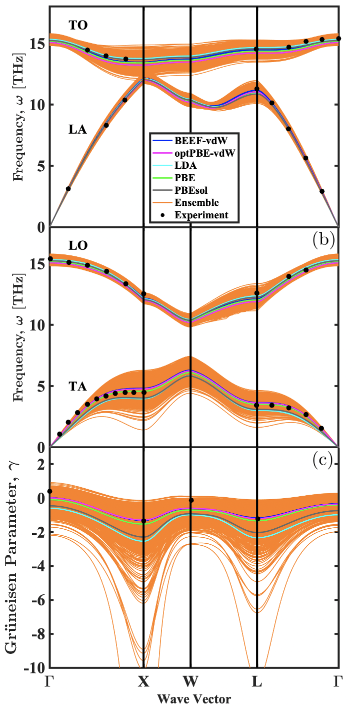
Figure 1: Silicon phonon dispersion relations for the (a) LA and TO branches and (b) TA and LO branches along high-symmetry directions. (c) Grüneisen parameters for the TA branch plotted along the same high-symmetry directions. The cut-off Grüneisen parameter curve reaches $-25$ at the $\mathbf{X}$-point. Experimental dispersion values are from Nilsson and NelinNilsson and Nelin (1972) and Grüneisen parameter values are from Madelung et al. Madelung et al. (2002) Each curve traces along the $\mathbf{\Gamma}$ $(0,0,0)$, $\mathbf{X}$ $(1,0,0)$, $\mathbf{W}$ $(1,0.5,0)$, and $\mathbf{L}$ $(0.5,0.5,0.5)$ reduced wave vector points in the Brillouin zone.

Specific heat values in units of J/kg-K are plotted in Fig. 2 as a function of temperature between $1$ and $1000$ K. Experimental values from Flubacher et al. Flubacher et al. (1959) are shown for comparison. The experimental data are bounded by the ensemble over the entire temperature range. The largest spread in the ensemble is $12$ J/kg-K at a temperature of $50$ K, which is 15% of the BEEF-vdW best-fit value of 76 J/kg-K at that temperature. As temperature is increased, $x=\hbar\omega/k_{\text{B}}T$ gets smaller, such that the differences in frequencies predicted by each ensemble are suppressed. This effect is reflected in the narrowing of the ensemble predictions above a temperature of 100 K. As the temperature approaches 1000 K, all ensemble and DFT self-consistent predictions approach the Dulong-Petit limit of $3k_{\text{B}}/m=888$ J/kg-K.

We also include the specific heat predicted using the Debye model,

$$c_{\text{Debye}}=\frac{9k_{\text{B}}}{m}\left(\frac{T}{\theta}\right)^{3}\int_{0}^{\theta/T}\frac{x^{4}e^{x}}{(e^{x}-1)^{2}}dx,$$ (9)

where $\theta=645$ K is the Debye temperature for silicon. Inyushkin et al. (2004) The Debye model prediction is worse than any of the ensemble predictions in the $30$ to $100$ K range, but is as accurate as any self-consistent calculation at temperatures below $10$ K and above $100$ K. The agreement at low temperatures is because the assumption of a linear dispersion relation for all phonons in the Debye model is most accurate at temperatures much lower than the Debye temperature. Inyushkin et al. (2004)

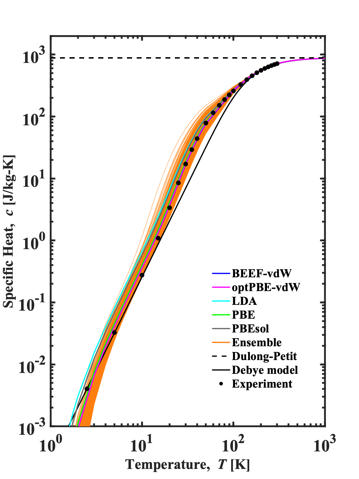
Figure 2: DFT and Debye model predictions of silicon specific heat. The Dulong-Petit limit is shown as a dotted line at $888$ J/kg-K. The experimental values are from Flubacher et al. Flubacher et al. (1959)

III.4 Grüneisen parameter and thermal expansion coefficient

The mode-dependent Grüneisen parameters quantify the effect of crystal volume change on the phonon frequencies and are a measure of anharmonicity. Jain and McGaughey (2015) We calculated them using the cubic force constants through Eq. (2) from Fabian and Allen. Fabian and Allen (1997) The results for the TA branch are plotted in Fig. 1(c) on the $\mathbf{\Gamma}-\mathbf{X}-\mathbf{W}-\mathbf{L}-\mathbf{\Gamma}$ loop. The remaining branches are plotted in Figs. S5(a)-S5(f). The TA branch at the $\mathbf{X}$-point has the largest spread of any of the modes, with a standard deviation of $1.00$. At the $\mathbf{X}$-point, the largest deviation of any self-consistent prediction from the BEEF-vdW value of $-1.31$ is the LDA value of $-2.54$.

The average Grüneisen parameter $\bar{\gamma}$ can be calculated as a specific heat-weighted average of mode Grüneisen parameters from

$$\bar{\gamma}=\frac{\sum_{\mathbf{q},\nu}c(\mathbf{q},\nu)|\gamma(\mathbf{q},\nu)|}{\sum_{\mathbf{q},\nu}c(\mathbf{q},\nu)}.$$ (10)

The average Grüneisen parameter predictions are reported in Table 1. BEEF-vdW and optPBE-vdW yield the lowest average value (0.92) and LDA yields the highest (1.16). All self-consistent predictions are bounded to within two standard deviations of the BEEF-vdW value. The differences in predictions of anharmonicity in both the self-consistent and ensemble calculations are correlated with the predicted thermal conductivity, an effect that we explore in Sec. III.6.

The mode-dependent Grüneisen parameters can be used to calculate the thermal expansion coefficient (TEC). Ritz et al. (2019) The ensemble TEC values for silicon are compared to the values from Guan et al.Guan et al. (2019) in Sec. S1E. While Guan et al. did not perform calculations for silicon, the coefficient of variation (COV $=$ standard deviation/mean) for the silicon TEC ensemble is $0.40$, consistent with the range of values they report (0.26 to 0.75). In contrast to our negatively-skewed silicon TEC distribution, however, all TEC distributions reported by Guan et al. have a positive skew.

III.5 Thermal conductivity

The thermal conductivity results are plotted in Fig. 3. The BEEF-vdW best-fit value is 171 W/m-K and the ensemble has a standard deviation of 24 W/m-K. The ensemble distribution is not symmetrical, with a longer tail to the left of its mean. A majority of ensemble functionals (1165 out of 2000) predict a lower thermal conductivity than the BEEF-vdW best-fit value. Following the procedure outlined by Guan et al. Guan et al. (2019) for fitting distributions based on the Cramer von Mises goodness of fit test, Anderson and Darling (1952) the distribution is best described ($p$-value $=0.94$) by a skewed normal distribution, which is also plotted in Fig. 3, with a mean of $190$ W/m-K, a standard deviation of $36$ W/m-K, and a skewness of $-3.7$. Additional distribution fits for other ensemble quantities are presented in Sec. S1E. The BEEF-vdW best-fit prediction is higher than the experimental value of 153 W/m-K. Inyushkin et al. (2004) An overestimation is reasonable because the prediction framework does not account for isotope, phonon-boundary, phonon-defect, or four-phonon scattering, all of which reduce thermal conductivity.

The BEEF-vdW ensemble bounds nearly all self-consistent DFT predictions, including those from Jain and McGaughey, Jain and McGaughey (2015) to within two ensemble standard deviations of the BEEF-vdW best-fit value. The largest discrepancy is the $122$ W/m-K thermal conductivity prediction from GPAW LDA ($-2.04\sigma$ from the BEEF-vdW value). There is no self-consistent thermal conductivity value in Table 1 greater than the BEEF-vdW best-fit functional prediction. It is noteworthy that the optPBE-vdW value of $165$ W/m-K is closest to the BEEF-vdW value. Parks et al. Parks et al. (2019) found that XC functionals that include vdW correlations, such as BEEF-vdW and optPBE-vdW, tend to predict higher vibrational frequencies for molecules and molecular complexes compared to GGA-level counterparts that do not include vdW correlations. A similar result is observed here in the BEEF-vdW and optPBE-vdW phonon dispersions in Figs. 1(a) and 1(b). BEEF-vdW and optPBE-vdW predict the highest $\mathbf{X}$-point frequencies for both the TA and LA branches, which results in higher group velocities and thus higher thermal conductivity.

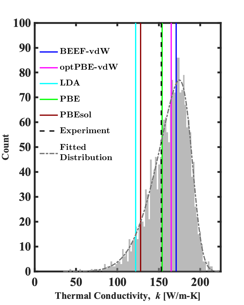
Figure 3: DFT predictions of silicon thermal conductivity at $T=300$ K, with the BEEF-vdW ensemble shown in gray. The lightest (middle) shade of gray indicates a range of $\pm\sigma$ ($\pm 2\sigma$) around the BEEF-vdW best-fit value. The experimental value is from Inyushkin et al. Inyushkin et al. (2004) The overlaid distribution is a skewed normal distribution with mean $190$ W/m-K, standard deviation $36$ W/m-K, and skewness $-3.7$.

The thermal conductivity accumulation function $k_{accum}(\Lambda)$ provides the contribution to thermal conductivity of phonons having mean free paths (MFP) less than $\Lambda$, where $\Lambda(\mathbf{q},\nu)=|\mathbf{v}_{g}(\mathbf{q},\nu)|\tau_{l}(\mathbf{q},\nu)$ for heat flow in the $l$-direction. McGaughey et al. (2019) The ensemble results are plotted in Fig. 4 as a heat map, with darker colors indicating a greater fraction of the ensemble predictions. The standard deviation of the ensemble thermal conductivity accumulation is also plotted. The experimental curve was determined by Cuffe et al.,Cuffe et al. (2015) who used a transient thermal grating technique to measure the thermal conductivity of single-crystal silicon membranes of varying thickness.

All functionals indicate that phonons with MFPs shorter than $10$ nm do not contribute to thermal conductivity. The ensemble accumulation functions spread widely between MFPs of $100$ to $300$ nm, a trend that is reflected in the sharp increase of the ensemble standard deviation in this range. The spread then remains uniform up to $10^{4}$ nm, the longest MFP considered. This result suggests that ensemble members that predict a high thermal conductivity overpredict the contributions of phonons with MFPs between $100$ and $300$ nm. This interpretation is consistent with the GPAW BEEF-vdW (171 W/m-K) and optPBE-vdW (165 W/m-K) predictions and with the findings of Jain and McGaughey, Jain and McGaughey (2015) who predicted a silicon thermal conductivity of $172$ W/m-K with the BLYP XC functional and attributed it to an overprediction of the contributions of $\sim 100$ nm MFP phonons. The experimental accumulation is bounded by the ensemble and has a similar slope compared to the self-consistent predictions, indicating agreement in the relative contributions of phonons with the displayed range of MFPs.

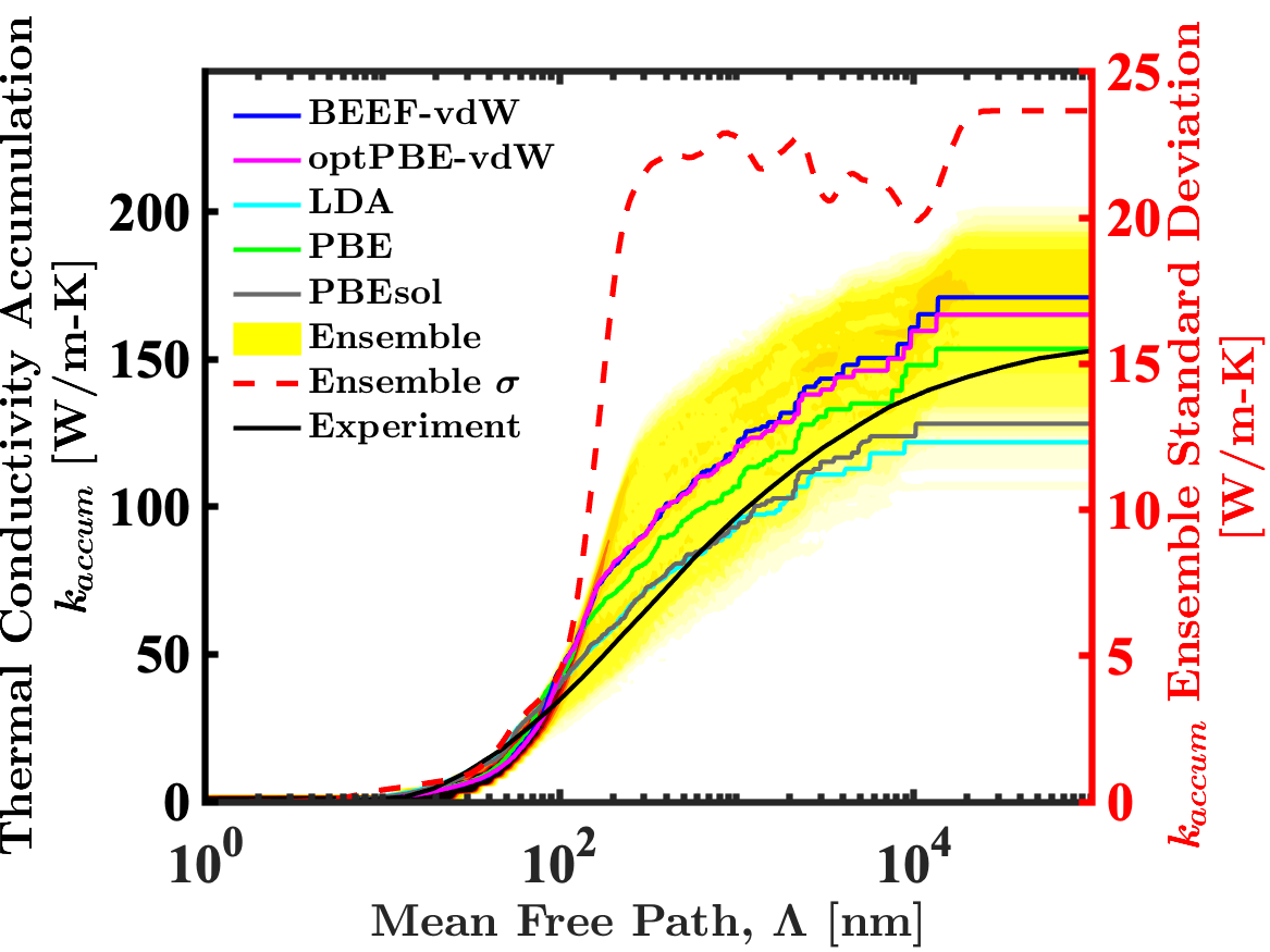
Figure 4: Self-consistent, ensemble, and experimental Cuffe et al. (2015) thermal conductivity accumulation functions of silicon at a temperature of $300$ K (left vertical axis). The red dotted line indicates the standard deviation of the ensemble thermal conductivity accumulation (right vertical axis).

In Sec. III.2, we noted an ambiguity in the choice of the lattice constant for the ensemble lattice dynamics and BTE calculations. The thermal conductivities plotted in Fig. 3 are calculated using the BEEF-vdW lattice constant. Choosing instead to use the ensemble lattice constants changes any individual thermal conductivity by at most $7$ W/m-K and has no effect on the ensemble thermal conductivity standard deviation. A histogram of thermal conductivity values calculated using the ensemble lattice constants is shown in Fig. S1(b). Based on the von Mises goodness of fit test ($p$-value $=0.97$), this distribution is also best described by a skewed normal distribution, with mean of $192$ W/m-K, a standard deviation of $38$ W/m-K, and a skewness of $-4.4$. This ensemble and its fitted distribution are nearly identical to the results obtained using the BEEF-vdW lattice constant shown in Fig. 3.

III.6 Thermal conductivity correlation analysis

(a)	(b)	(c)
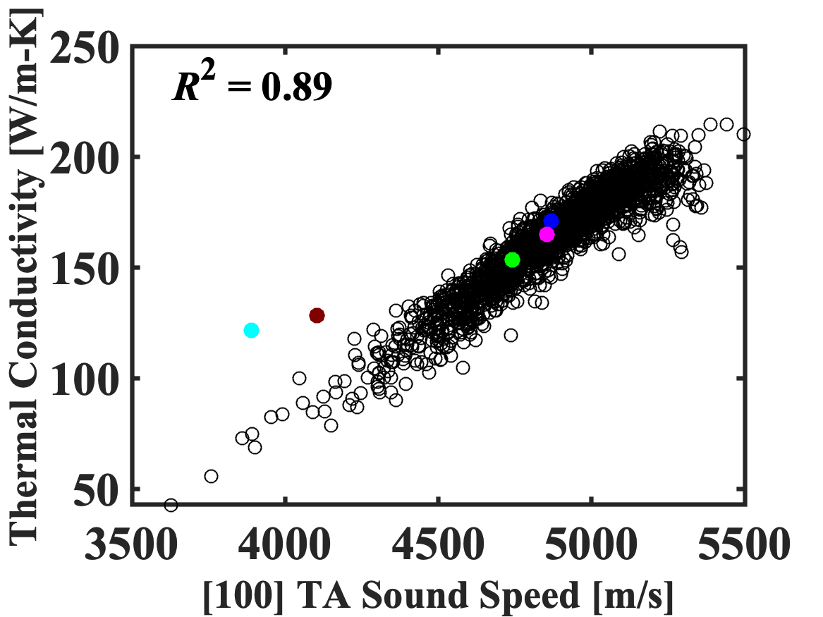
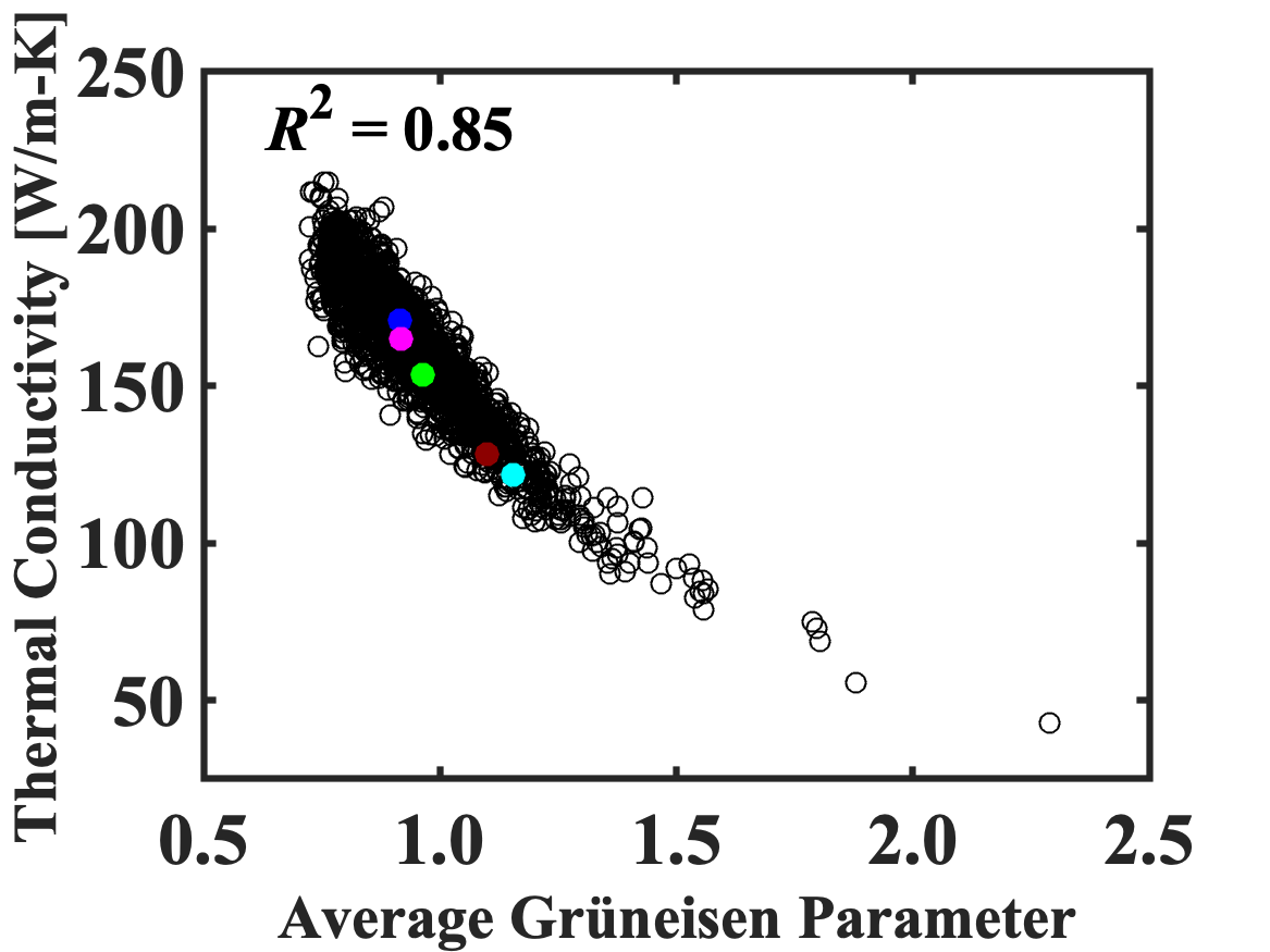
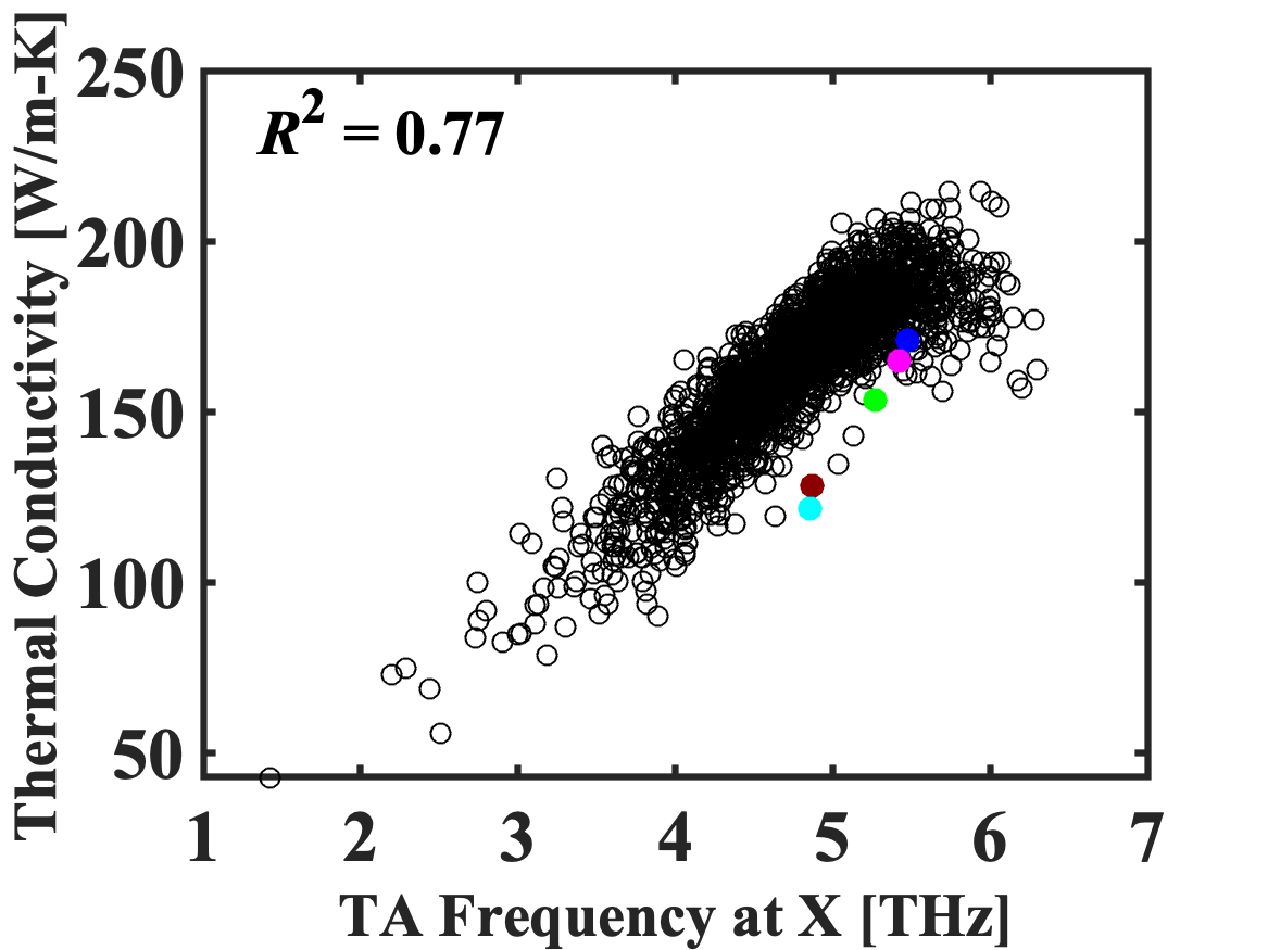
(d)	(e)	(f)
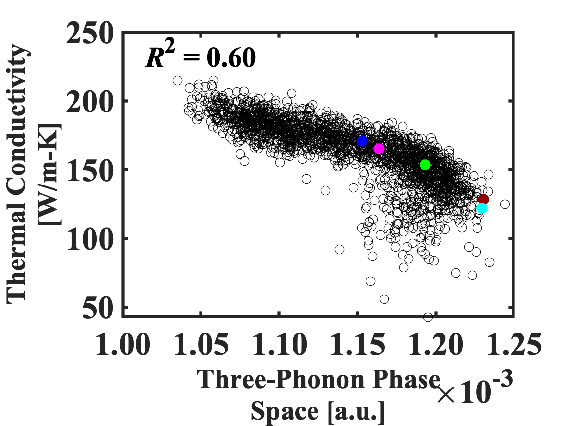
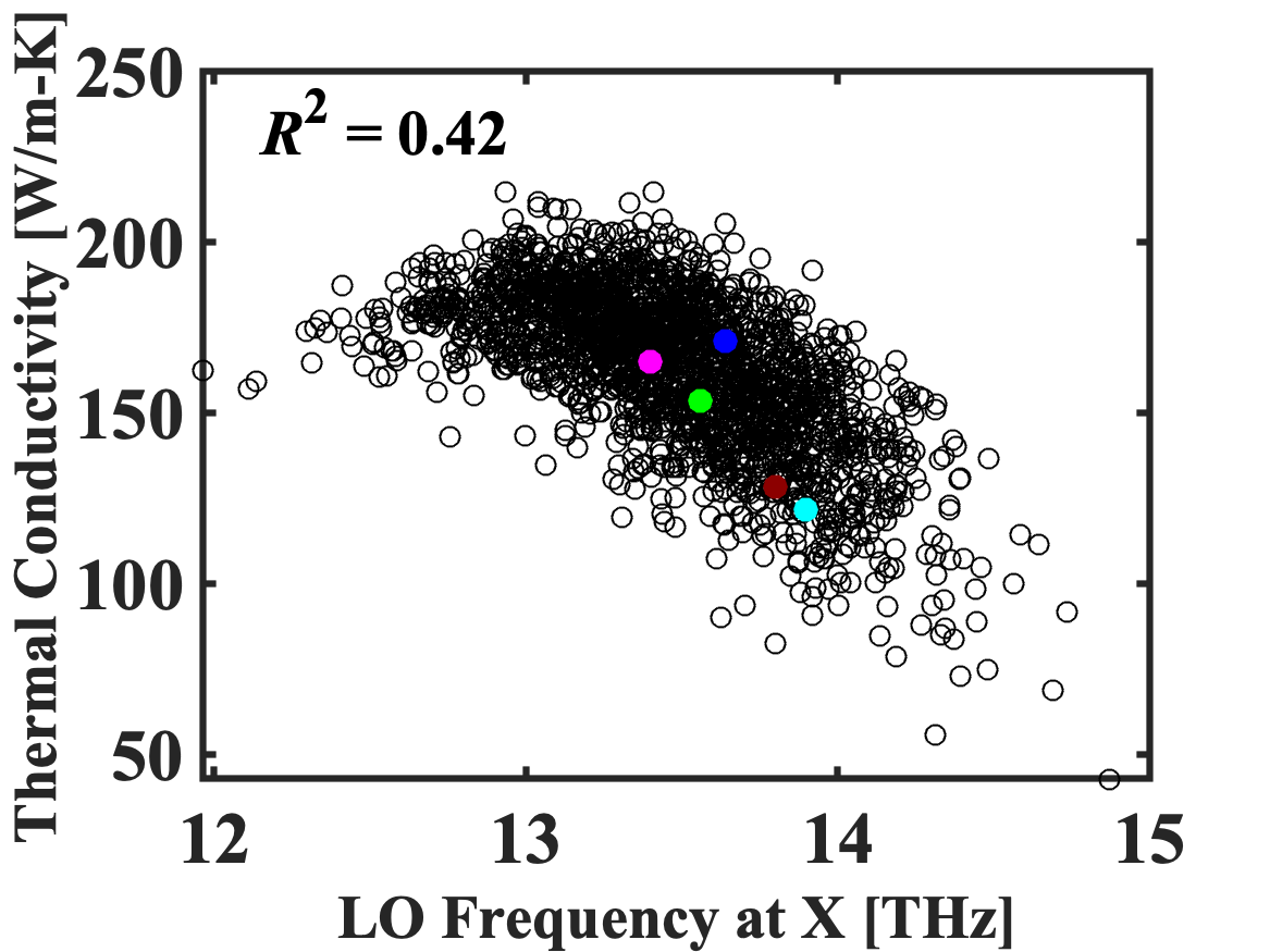
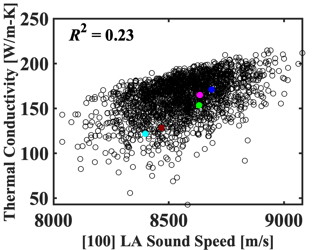
(g)	(h)

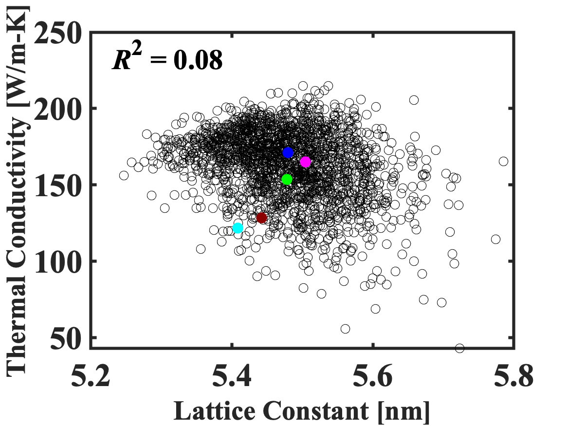
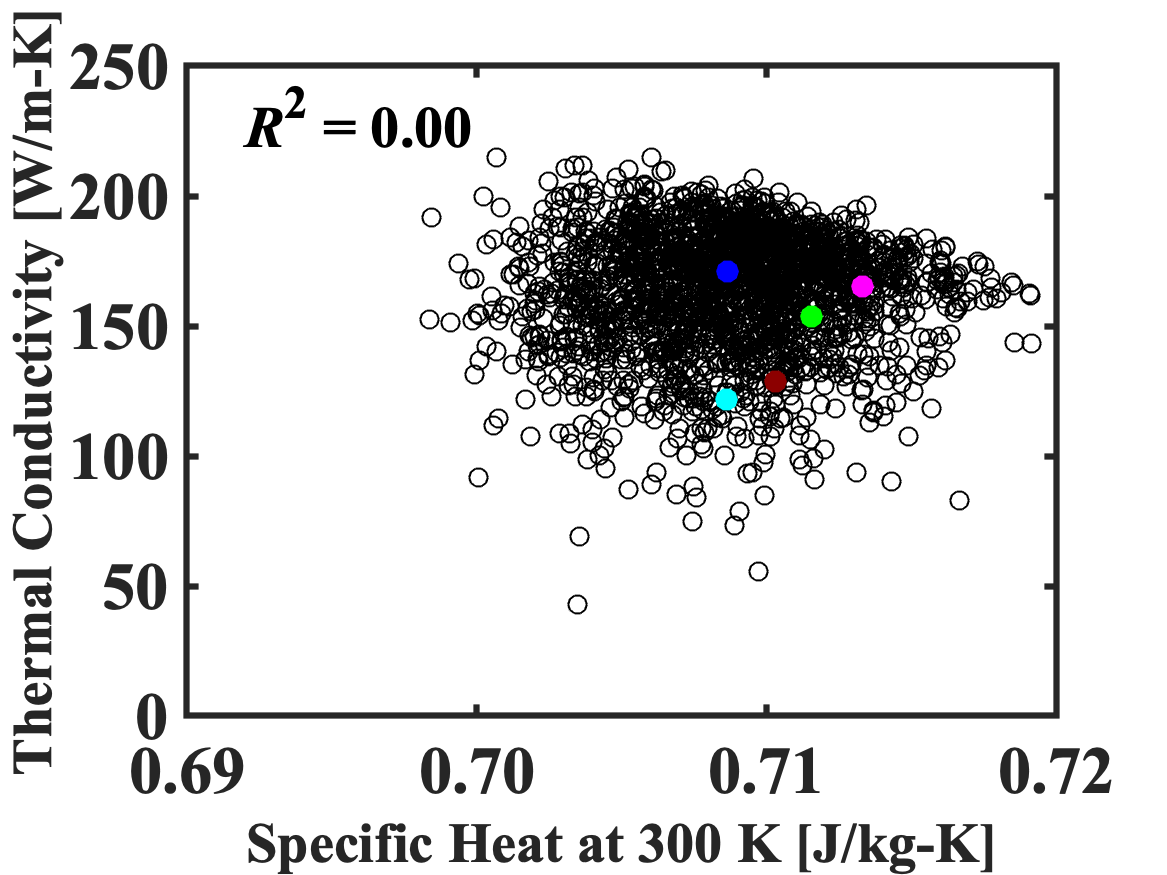
Figure 5: Correlation of the BEEF-vdW ensemble predictions of thermal conductivity at $T=300$ K with other phonon and structural properties. The panels are presented in decreasing order of $R^{2}$. The quantities are (a) [100] TA sound speed, (b) average Grüneisen parameter, (c) $\mathbf{X}$-point TA frequency, (d) three-phonon phase space, (e) $\mathbf{X}$-point LO frequency, (f) [100] LA sound speed, (g) lattice constant, and (h) specific heat at $T=300$ K. Self-consistent predictions are denoted with colored markers.

We now examine how the spread in the ensemble thermal conductivities is related to the spreads in other ensemble quantities. The results are shown in Figs. 5(a)-5(h) as scatter plots in order of decreasing coefficient of determination, $R^{2}$. The best predictors of thermal conductivity are the $[100]$ TA branch sound speed ($R^{2}=0.89$), the average Grüneisen parameter ($R^{2}=0.85$), and the TA branch $\mathbf{X}$-point frequency ($R^{2}=0.77$). It is not surprising that these quantities are strong predictors of the thermal conductivity, as the TA branch has a high group velocity and the Grüneisen parameter is a measure of anharmonicity. An initially surprising result is that the $[100]$ LA branch sound speed is a poor predictor of thermal conductivity ($R^{2}=0.23$), as LA phonons, like TA phonons, have high group velocities. The LA sound speed is likely a poor predictor because there is not enough spread in the ensemble predictions to account for the variation in the thermal conductivity ensemble predictions. the COV for the LA sound speed is $0.019$, while that for the TA sound speed is $0.048$.

The worst predictors are the specific heat at a temperature of $300$ K ($R^{2}=0.00$) and lattice constant (R${}^{2}=0.06$). As with the LA sound speed, both the specific heat ($\sigma=4$ J/kg-K, COV$=0.005$) and lattice constant ($\sigma=0.077\text{ }\text{\AA}$, COV$=0.014$) have small standard deviations and thus make a minimal contribution to the $24$ W/m-K standard deviation and 0.14 COV of the thermal conductivity ensemble. The low correlation of the lattice constant and thermal conductivity is consistent with our observation that the lattice constant used in the lattice dynamics calculations does not significantly impact the behavior of the thermal conductivity ensemble.

It is instructive to compare Figs. 5(c) and 5(e), which plot the thermal conductivity versus the frequency of the TA and LO branches at the $\mathbf{X}$-point. These two dispersion branches have large frequency spreads at the $\mathbf{X}$-point. The TA branch has a standard deviation of $0.57$ THz and that of the LO branch is $0.39$ THz. The TA frequency at the $\mathbf{X}$-point, however, is a better predictor of the thermal conductivity ($R^{2}=0.77$) than the LO $\mathbf{X}$-point frequency ($R^{2}=0.42$). Because the LO group velocities are small, they do not make a significant contribution to the thermal conductivity, so that it is not surprising that there is a weak correlation between these quantities.

A quantity that we anticipated would be correlated with thermal conductivity is the three-phonon phase space, which is defined in Sec. S4. Although the three-phonon phase space is purely a harmonic property, Lindsay and Broido showed that it is inversely correlated to the thermal conductivity of several semiconductors including silicon, Lindsay and Broido (2008) indicating that materials with fewer available scattering processes tend to have higher thermal conductivities. As shown in Fig. 5(d), there is an inverse correlation between the ensemble phase space and thermal conductivity for silicon, but the qualitative behavior is different from that observed by Lindsay and Broido. There is only an inverse correlation for thermal conductivity predictions above $150$ W/m-K ($R^{2}=0.65$), while the correlation is weak for predictions below $150$ W/m-K ($R^{2}=0.02$). The five self-consistent XC functionals follow this relationship, with two functionals (LDA and PBEsol) lying in the lower range and the other three (BEEF-vdW, optPBE-vdW, and PBE) lying in the upper range.

IV Conclusion

We presented a computationally-efficient framework that uses the BEEF-vdW ensemble to quantify the uncertainty due to XC functional choice in predictions of phonon properties and lattice thermal conductivity. We applied this framework to isotopically-pure silicon, a popular benchmark of ab initio predictions of thermal conductivity. As summarized in Table 1, we found that the BEEF-vdW best-fit value bounds most of the self-consistent predictions to within two ensemble standard deviations. This agreement encompasses harmonic quantities such as the phonon frequencies [Figs. 1(a) and 1(b)], specific heat (Fig. 2) and the three-phonon phase space, as well as properties that require incorporating anharmonic effects like the thermal conductivity (Fig. 3) and the average Grüneisen parameter.

In addition to quantifying the XC uncertainty, our results provide insight into the way that DFT at the GGA-level describes the phonon dynamics in silicon. We found, for example, that the greatest spread in ensemble dispersions occurs at the $\mathbf{X}$-point in the TA branch, in agreement with previous works that found accurate prediction of phonon frequencies in that part of the Brillouin zone to be challenging. We found that ensemble functionals vary widely in their descriptions of phonons with mean free paths between $100$ and $300$ nm, and that these variations are correlated with predictions of thermal conductivity (Fig. 4). As shown in Fig. 5, we were able to use the ensemble to identify the [100] TA sound speed and the average Grüneisen parameter as good predictors of thermal conductivity. Conversely, we found that the specific heat and [100] LA sound speed, which are described consistently amongst the ensemble members, are poor predictors of the thermal conductivity despite being essential components of the calculation. Because our framework can be used to examine the predictions of thousands of XC functionals, it can be applied in the future to identify trends in phonon dynamics that occur due to, or in spite of, the choice of XC functional in other materials.