D-22761 Hamburg, Germany
Analytic structure of the 8-point scattering amplitude in multi-Regge kinematics
in SYM :
conformal Regge pole and Regge cut contributions111This paper is dedicated to the memory of L.N.Lipatov who has initiated this line of research and provided essential contributions
Abstract
Continuing our investigations of the analytic structure of the scattering amplitudes in the planar limit of SYM in multi-Regge kinematics we compute, in all kinematic regions, the Regge cut contributions of the process in leading order. Compared to previous studies of the and the processes we encounter two new features: the 3-reggon cut and the product of two 2-reggeon cut contributions.
1 Introduction
It is now well established that the Bern-Dixon-Smirnow (BDS) conjecture Bern:2005iz for the MHV n-point scattering amplitude in the planar limit of the SYM theory is incomplete for . One of the first indications for this was found in Bartels:2008ce ; Bartels:2008sc . Corrections to the BDS-formula have been named ’remainder functions’, , and in recent years major efforts have been made for determining these remainder functions, in particular the remainder function for the case and Bartels:2013jna ; Bartels:2014jya . The function has been calculated for two, and three loops Goncharov:2010jf ; Lipatov:2010ad ; Bartels:2010tx ; DelDuca:2009au ; DelDuca:2010zg ; Dixon:2011pw ; Dixon:2011nj ; Dixon:2012yy ; Pennington:2012zj ; Dixon:2013eka . More recently new techniques have been developped and applied to calculate higher loops Bargheer:2015djt ; DelDuca:2018hrv ; DelDuca:2018raq ; Caron-Huot:2019vjl ; Bargheer:2019lic ; DelDuca:2019tur .
In order to fully analyse and to go beyond this loop expansion, it has turned out to be useful to consider special kinematic limits, in particular the multi-Regge limit. The benefit of considering this special region is the particular analytic structure of the scattering amplitudes, in particular the Regge factorization. This stucture is expected to be valid to all orders: the higher order calculations mentioned before can therefore be compared and analyzed. In subsequent papers Bartels:2013jna ; Bartels:2014jya the analytic structure of the and the scattering amplitudes has been investigated, making use of Regge theory and unitarity, and in the leading logarithmic approximation the Regge pole and Regge cut contributions have been computed in all kinematic regions.
The present paper extends these calculations to the amplitude. This 8-point function is of particular interest since it exhibits, for the first time, a Reggeon cut contribution consisting of three reggeized gluons. In Lipatov:2009nt it was found that the Hamlitonian of the Regge-cuts belongs to an integrable open Heisenberg spin chain. Regge-cuts composed of reggeized gluons probe the spin chains consisting of sites. In the and scattering amplitudes only the shortest spin chain, consisting of two sites, appears; spin chains with three sites appear first in the scattering amplitudes, spin chains of 4 sites in the amplitude etc. In this paper we compute the partial waves of the amplitude containing the 3-gluon cut. The energy spectrum of the Hamiltonian of the three gluon state has first been addressed in Lipatov:2009nt . Another novel feature of the amplitude is the repetition of Regge cuts: the short cut which was found in the amplitude, now can appear twice, in the channel and in the channel.
Technically speaking the amplitude requires new fatures. First, when using unitarity for the computation of Regge cut amplitudes, the new terms (Regge cuts consisting of three reggeized gluons, and the product of two short cuts) now require double and even higher order discontinuities, even for the leading logarithmic approximation. This provides a crucial test of the analytic structure, based on the Steinmann relations. Second, the calculation of subtraction terms now becomes more complicated. In Bartels:2008ce ; Lipatov:2010qf it had been pointed out that the planar approximation, when applied to the Regge limit of SYM theory, leads to a new feature which requires special attention. As it is well known, Regge theory (Carlson theorem) requires the definition and use of signatured amplitudes. Once signature has been introduced, in the Regge pole approximation multiparticle production amplitudes factorize. For QCD this has been verified in the context of the BFKL equation. In the planar approximation (leading order large ), however, there is no space for signature: hence the study of the Regge limit of SYM theories in the planar approximation raises the question how much of the known Regge structure remains applicable. As a first consequence of the absence of signature, it has been observed in Bartels:2008ce ; Lipatov:2010qf that, in the Regge pole approximation, the factorization of multiparticle production amplitudes is violated in certain kinematic regions. This violation is accompanied by the appearance of unphysical singularities. It was then noticed that these singular pieces appear in exactly the same kinematic regions where also the Regge cut contributions contribute, and they also have the same phase as the Regge cut contributions. Hence they can be removed by re-defining the Regge cut contributions by introducing subtractions terms. In previous papers this was shown for the and the amplitudes. In the present paper we show that such subtractions can be found also for the amplitude. This suggests that in the planar lapproximation of SYM theories, despite the absence of signature, the general structure of Regge amplitudes remains valid.
2 Outline of the strategy
Let us first indicate how our calculations will be performed. We will make use of the
method developed in our previous papers on the 7-point function Bartels:2013jna ; Bartels:2014jya , and wewill proceed in several steps:
(1) We describe the decomposition of the scattering amplitude into a sum of
several pieces, where each term, in accordance with the Steinman relations, is characterized by a maximal set of non-overlapping energy discontinuities. In the present case we have
a sum of 42 terms, and each term has a set of five nonoverlapping energy discontinuities.
(2) In the planar approximation, each term in this decomposition contains a product of energy factors, the phases of which depend upon the kinematic region. Our list applies to the region where all energies are positive.
(In the case of signatured amplitudes one would have to form linear combinations of differenz kinematic regions).
(3) Whereas the Regge poles contribute to all 42 terms in this decomposition, the Regge cuts appear in specific
terms only. Since each Regge cut can be computed from a specific set of energy discontinuities, for each term of the decomposition the content of energy discontinuities allows to decide, which of the Regge cuts might contribute.
(4) Regge pole and Regge cut contributions are accompanied by trigonometric factors which have their origin in the
partial wave expansion. For the 7-point amplitude the method of finding these factors has been described in Bartels:2013jna ; Bartels:2014jya , and it is not difficult to extend these rules also to the present case (the sum of the Regge pole contributions can also be
derived from the BDS formula Bartels:2013jna ).
It is due to these trigonometric factors that, in certain kinemtaic regions, unphysical singularities appear.
(5) Focussing now on specific kinematic regions and inserting the corresponding phases of the energy factors, one finds extensive cancellations. It is these cancellations which
let the Regge cut terms appear only in specific kinematic regions.
(6) As we have said already, the Regge pole terms come with unphysical singularities in exactly the same kinematic regions where also Regge cut terms
appear. It is this coincidence which has suggested to introduce subtractions for the Regge cuts in such a way that the singularities are cancelled.
For the present case the determination of the subtractions is lengthy and rather technical, and we move it into the Appendix D. .
(7) Once the necessary subtractions of the Regge cut conributions have been found, the representation found in the previous steps can be modified and all singularities arising from the trigonometric factors will be removed.
We believe that the success of finding these subtraction which consistently remove the singularities represents an important confirmation of the correctness of our procedure.
(8) Once we know the form of the scattering amplitude
we can use energy discontinuities
(single and a few higher order energy discontinuities) to determine the individual Regge cut pieces.
It is important to note that, up to this point, the results are expected to be valid to all orders: the form of the scattering amplitude as well as the energy discintinuity relations.
(9) The final step is the calculation of the Regge cut terms, based upon the energy (single or double) discontinuity equations and unitarity. The evaluation of the unitarity equations will be restricted to the leading logarithmic approximation. Most of the ingredients necessary for a NLO calculation are known and can be used,, but this will not be attempted in the present paper.
Our paper is organized as follows. First (section 3) we discuss the analytic structure (steps (1)- (3)). The trigonometric factors are listed in Appendix B, and the sum of the Regge pole terms is given in Appendix C. In section 4 we discuss, for the simplest case of the short Regge cut, the problem of subtractions. In the following two sections we then go through the different Regge cut contributions and list the kinematic regions where they appear: section 5 for the short and long cuts, section 6 for the very long cut, the double cut and the 3-reggeon cut. In each of these sections, we begin with the representation which directly follows from section 3 and the trigonometric factors contained in the Appendices and still contains singularities. Using then the subtractions derived in Appendix D we obtain the regular representation. In section 7 we compute the energy discontinuities which will allow to find the partial waves. The final step then is the computation of the corresponding unitarity integrals where we will restrict ourselves to the leading logarithmic approximation. Section 8 contains our (leading order) results for the very long cut, the 3-reggeon cut and the double cut in the different kinematic regions. Finally, in section 9 we give a brief summary and outlook.
3 The Analytic structure
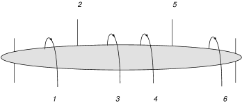
We begin with the analytic structure of the amplitude in the multiregge region (steps (1) and (2) of the previous section). Our notation is illustrated in the following figure:
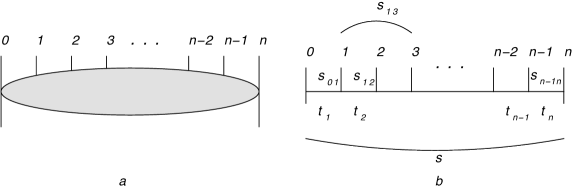
In the following we will label the four produced particles also by ,,,.
3.1 Decomposition
We write the (unsignatured) scattering amplitude in the multi-Regge kinematics as a sum of 42 terms:
| (1) |
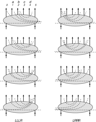
Each term belongs to a specific set of five simultaneous energy discontinuities in non-overlapping channels. We group these terms into five singlets, three doublets, four triplets, two quartets, a singlet, and a sextet. Below we illustrate the discontinuity structure and list the energy factors. Here ,where denotes the angular momentum in the channel, and . First the singlets:
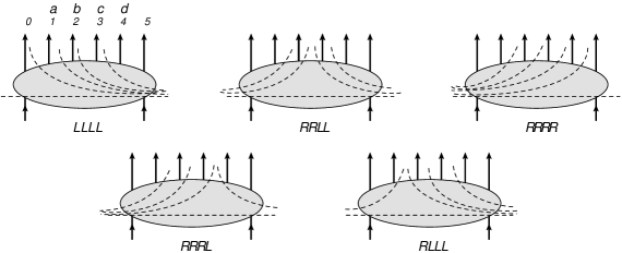
The corresponding energy factors are (in the kinematic region where all energies are positive):
| LLLL | (2) | ||||
| RRLL | (3) | ||||
| RRRR | (4) | ||||
| RRRL | (5) | ||||
| (6) |
Next the three doublets:
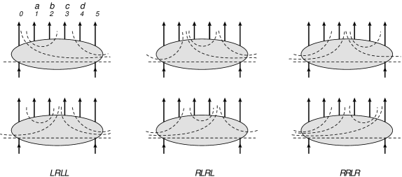
| (7) |
| (8) |
| (9) |
The triplets are of the form:
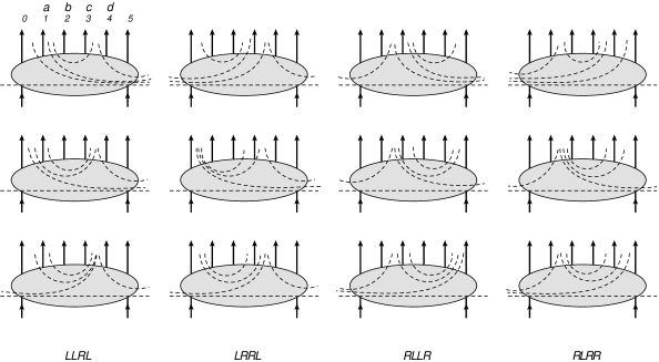
| (10) |
| (11) |
| (12) |
| (13) |
Next the two quartets:
| (14) |
| (15) |
The quintet has the form (here the numbering 1..5 goes from left to right starting from the upper left diagram):
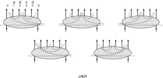
| (16) |
Finally the sextet (the numbering 1..6 is contained in the figure. The diagrams in the lower line are the mirror reflections of the upper line):
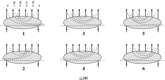
| (17) |
As it can be seen from Fig.2 - 7, each term can be characterized by a set of 4 subscripts ’L’ or ’R’. Beginning with the left-most produced particle, the first subscript distinguishes whether the energy discontinuity line comes from the left or from the right. The second subscript says the same for the second produced particle, and so on. A closer look at Fig.2 - 7 shows that these labels are not sufficient: depending on the discontinuity structure, we still have singlets, doublets etc.
For each term, the product of energy factors clearly reflects the non-overlapping multiple energy discontinuities. Often it is more convenient to rewrite these energy factors in a factorizing form. Using identities such as
| (18) |
it is then straightforward to see that in all terms the energy factors (disregarding the phases) can be written as the product
| (19) |
In the product of factors the exponents depend upon the subscripts ’L’ or ’R’: for each produced particle labelled by ’L’ or ’R’: we have or , resp. As an example, terms labelled by LLLL come with the product
| (20) |
In leading order, we can put these factors equal to unity.
From now on we introduce a small change of our notation. Instead of we now will use, as integration variable, , and the unprimed variable
| (21) | |||||
will be used for the reggeon trajectory function in the channel: .
3.2 A few general remarks on the formulae of the scattering amplitude
For each term we have a Sommerfeld-Watson integral. A more detailed discussion has been given in our previous paper Bartels:2014jya . Each term is written in the form:
| (22) | |||||
where The are real-valued, and they contain, in addition to the trigonometric factors to be discussed below, the partial waves. Each is written as a sum of several pieces which contain Regge pole or Regge cut singularities:
| (23) |
In order to obtain a signatured amplitude we have to form linear combinations of crossed and uncrossed amplitudes. This amounts to replacing the phase of the energy factor by a signature factor , e.g.
| (24) |
Instead, in the planar approximation the product of signature factors is expanded in products of the , and each term denotes a particular kinematic region. For example, the term without any denotes the region where all energies are positive, the term the region where the channel has been twisted etc. In the following we will use this notation for labelling the different kinematic regions.
We are interested in the corrections to the BDS expression for the scattering amplitude, depending on the kinematic region.. For each region we write the scattering amplitude in the form
| (25) |
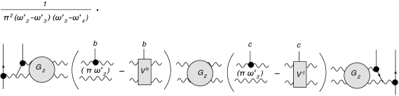
Here the BDS part contains the Regge pole part illustrated in Fig8:

consisting of the energy factors (without phases) , the real valued couplings to the external incoming particles, the absolute values of the production vertices, and the two phase factors:
| (26) |
Here the contain the one loop Regge cuts, and in Appendix A we give a list of the phases for all kinematic regions which contain Regge cuts. In this notation, our discussion will focus on the product
| (27) |
and the remaining factor will be called the ’BDS’ part. In our leading approximation, the exponential will be expanded. The same convention will be used when we discuss energy discontinuities: the BDS part will be extracted and not written explicitly.
The integral representation (22) contains, for each -channel, the integral over the corresponding angular momentum . If, for a given kinematic region , the -channel has only a Regge pole contribution, the integral can be done directly and leads to a factor where denotes the gluon trajetory in the channel (21). If the -channel has a Regge cut contribution, the corresponding can be shifted:
| (28) |
and in this way also produces a factor (a more detailed discussion of this shift will be given in section 5.1). As a result, all energy factors contained in the BDS part will be factored out from our scattering amplitudes, derived in this paper, leading to the expression (27).
Finally we address the question which Regge pieces contribute to each of the 42 terms. As we have said before, each Regge pole or cut term comes with a product of trigonometric factors, resulting from the partial wave expansions in the various -channels. Detailed rules and their application to the scattering process have been given in the appendix of Bartels:2014jya , and it is not dificult to generalize to the process. A complete list of these trigonometric factors is given in Appendix B: for each of the 42 terms in our decomposition we list the trigonometric factors of the Regge pole and cut contributions. Regge poles appear in all terms, Regge cuts only in those terms which contain the set of energy discontinuities related to the Regge cut. As an example, the very long two-reggeon cut in the , and channel can appear only in those terms which have an energy discontinuity in :
| (29) |
In order to find out in which kinematic region a given Regge cut contribution appears, we combine the trigonometric factors of this Regge cut and the phases coming from the energy factors of this kinematic region, and take the sum over all of the 42 terms which contain this Regge cut. As a result, one finds many cancellations, and at the end the Regge cut, if at all, appears only in very specific kinematic regions. As one general result we mention that, both in the region where all energies are positive and in the purely euclidean region, all Regge cut contributions cancel. On the other hand, the Regge poles appear in all kinematic regions, and a complete list of their contributions is given in Appendix C.
There exist important consistency checks. Beginning with the Regge pole contributions, the obtained results which are listed in Appendix C can be compared with the pole expressions derived from the BDS formulae (as outlined in Bartels:2013jna ). One finds complete agreement. As to Regge cuts, in the appendix of Lipatov:2009nt arguments have been given that, in the planar approximation, Regge cuts can appear only if some of the produced particles are continued to the region of negative energies. As an example, in the amplitude the two reggeon cut in the channel contributes only if both the and channels are twisted, i.e. both produced particles have to be continued to have negative energy. In the amplitude, the very long Regge cut requires twists in the and channels.
In the following we will consider the different kinematic regions. We find it convenient to discuss the different cut contributions seperately. Beginning with the region where only one short Regge cut (one t-channel) contributes, we then address the regions with a long cut (two t-channels), and finally come to the regions where the very long cut (three t-channels), the double cut and the three reggeon cut appear.
4 The problem of subtractions
Before we begin with the different kinematic regions we say a bit more about the problem of subtractions. As we have already said before, the planar approximation leads to a problem which requires special attention. For this we return to the Regge pole contributions. As discussed in Lipatov:2010qf ; Bartels:2013jna , starting from the BDS formula one finds that the Regge pole contributions become singular in all those kinematic regions where Regge cut contributions appear, and these singularities have the same phase structure as the Regge cuts. This suggests to re-define the Regge cut by a subtraction term which removes the singularity. For illustration we go to Appendix C where we have listed the pole contributions of the amplitude for all kinematic regions. Their form can be derived from the BDS formula; alternatively we could also start from Appendix B and compute the sum of the pole contributions in the different regions. The table begins with those regions which have no Regge cuts, and the pole contributions are just phase factors. In all subsequent regions, the pole conributions contain singularities.
To be definite, let us consider the regions and , in which only the short 2-reggeon cut in the -channel contributes. In this region the Regge pole contribution in Appendix B is of the form:
| (30) |
which we can also write as
| (31) |
Here we have used:
| (32) | |||||
| (33) |
and as discussed before, the BDS part has been removed (in particular the energy factors of fhe Regge poles). Similarly for the region :
| (34) |
In (31) and (34) it is the brackets, in particular the terms proportional to , which are unphysical and should be removed by the Regge cut in the channel, .
For the sum of all terms containing the short Rdegge cut we obtain after some algebra, before the integration over
| (35) | |||||
| (36) |
Next we include, for the Regge cut amplitude, the integral with the energy :
| (37) |
with
| (38) |
Here we have perfomed the shift discussed in (28), and extracted the factor . It belongs to the BDS part, and in the following we will disregard it.
Now the Regge cut part has the same phase structure as the singular pieces of the Regge pole term. In order to cancel these singular pieces we put
| (39) |
with
| (40) |
With this subtraction we obtain for the sum of the Regge pole and the short Regge cut
| (41) |
The first term in the square brackets defines the conformal infrared finite Regge pole contribution in this kinematic region. In the same way we find for the region (using the same subtraction ):
| (42) |
Obviously, is a subtraction term of the -integral in the angular momentum plane.
For simplicity, we write (39) in the short hand notation
| (43) |
i.e. we will not explicitly write the integral and the energy variables multiplying or .
It is important to keep in mind that these singular terms also appear in the energy discontinuity relations. For simplicity we consider the discontinuity in in the region of positive energies:
| (44) |
Here
| (45) |
Again the singularity of the Regge pole term appears. By inserting (39) and (40), also this discontinuity becomes regular:
| (46) |
It should be stressed that the singularity in the Regge pole terms (31) and (34) woukd cancel if, instead of considering the regions and separately, we would form odd signatured amplitudes.This demonstrates that it is the planar approximation which is connected with the appearance of these singularities.
The simple case of the short cut in the -channel generalizes to all kinematic regions where Regge cuts appear: the Regge pole contributions have singular tems which have to be cancelled by subtractions of Regge cut contributions
| (47) |
Here we will use the shorthand notation discussed after (43).
For the cases and the subtraction terms have been found and discussed in previous papers. For the present case it is one of the main challenges to find the subtraction terms for the new Regge cut conributions and to verify that, with these subtractions, both the scattering amplitudes and the energy discontinuities become regular.
5 The cut contributions of the short and the long Regge cuts
We now determine the Regge cut contributions. We will go through the Regge cuts (short, long, very long, double cut, three reggeon cut) in the different kinematic regions and combine, for each region, the phases from the energy factors listed in the prevous section with the trigonometric factors listed in Appendix B and C. These calculations are lengthy and are done using Mathematica. The results, however, become simple. In the next step we decompose the partial waves :
| (48) |
and compute the singular pieces, , from the requirement that they cancel the unphysical singularities of the Regge pole contributions. We then find the amlitudes containing only regular terms. In the next step we write down equations for the energy discontinuities, inserting the necessary subtractions. Finally, we use unitarity equations (restricting ourselves to the leading logarithmic approximation) and find explicit expressions for the Regge cut contributions.
5.1 The short cuts
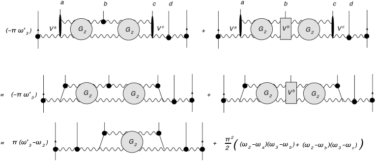
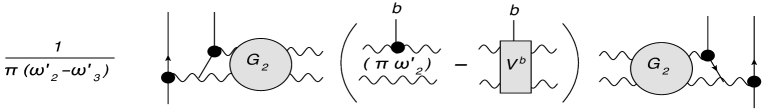
We begin with the Regge cut contributions in the channel and conisder the regions and . This region has been discussed already in the last section, and we only need to compute the energy discontinuity in (46). First we write the equation in the leading approximation:
| (49) |
For the computation of the discontinuity on the lhs we use unitarity (Fig.9a):

and for the unitarity integrals we restrict ourselves to the leading log approximation. In leading order the production vertices in Fig.9 simplify:

In particular, in (a) the production vertices at the lhs end of the cut is a sum of a pointlike vertex and and a vertex involving a particle propagator. In the following this latter part will be denoted by . With this the result is:
| (50) |
where we have used
| (51) |
with etc. Here the first three terms denote the one loop contributions, and the leading order function which is illustrated in Fig.11 a starts from 2 loops::

Before we continue we come back to the shift in the which we have discussed in section 3.2. The rungs in Fig.9 denote the BFKL kernel in the octet representetion which we write as Bartels:2008sc :
| (52) | |||||
The new kernel has the important bootstrap property .
| (53) |
In the ladder diagrams of Fig.11a the Green’s function satisfies the equation
| (54) |
Writing its solution in the simplified form :
| (55) |
we see that, when performing the -integral, we can shift the integration variable
| (56) |
and obain an extra factor
| (57) |
This factor belongs into the BDS part and, therefore, will be disregarded (as it has already been done in (46) and (49) ). In the following this shift applies to all 2-reggeon cut confributions, and whenever we encounter an -integration it is understood that the corresponding energy factor will be disregarded since it has been absorbed by the BDS part of the scattering amplitude.
Returning now to (50) we have for the following analytic representation in the -representation (Fig.9a).:
| (58) |
where we have subtracted the infrared divergent one loop integral, . It is convenient to introduce, in the infrared finite and conformal invariant phases:
| (59) |
which leads to the result for the unitarity integral:
| (60) |
With this unitarity integral we return to (49) and obtain the conformal invariant result for the short Regge cut in the channel:
| (61) |
Our final result for the weak coupling limit thus becomes:
| (62) |
We remind that this result represents, to leading order, the combination (27). In order to obtain the complete scattering amplitude we still have to multiply by the BDS part, i.e.the product of the Regge pole factors, , and by the couplings to the external particles.
The analogous results for the short cuts in the and are easily obtained by suitable changes of variables.
5.2 Long cuts
Turning to the long cuts in the and channels we notice that the phase structure suggests, instead of the long cut amplitudes etc., to define real-valued combinations of long and short cut contributions. We therefore introduce the modified long cut amplitudes:
| (63) | |||||
| (64) |
and
| (65) | |||||
| (66) |
with
| (67) |
Moreover, for later purposes it will be convenient to introduce the following short hand notation:
| (68) |
With these notations we find the following cut contributions:
| (69) | |||||
| (70) | |||||
| (71) | |||||
| (72) | |||||
The corresponding pole contributions are listed in Appendix C.
In (69) - (72) we have used a short hand notation which we have to explain. In order to obtain, for example, (69) we proceed as follows. We start from the integral of the form (22) which we write as
| (73) | |||||
where is a sum of Regge pole and Regge cut terms As said before, each Regge cut term comes with angular momentum integrals for all t-channels over which the cut extends. For the long cut discussed now the and channels are involved, i.e. the we have the integration
| (74) |
All other variables can be substituted by the corresponding Regge pole Also the phases are written as primed, i.e. for the first term in (69) we have
| (75) |
After the shift this becomes
| (76) |
The energy factors in front of the integral belong to the BDS part and will be disregarded, and we are thus left with
| (77) |
This should explain our short hand notation ’’. Throughout the main part of this paper we will make use of this notation.
The determination of the singular pieces has been described in Appendix B and will not be repeated here. As the main result, we have found real-valued terms , which remove the singularities in all kinematic regions. Adding Regge pole and cut contributions and inserting the subtractions
| (78) | |||||
| (79) |
we arrive, for the sum of Regge pole and Regge cuts, at the finite expressions:
| (80) | |||||
| (81) | |||||
| (82) | |||||
In the following we will use energy discontinuities and unitarity to compute the Regge cut amplitudes. Since the evaluation of the unitarity integrals will be done only in the leading logarithmic approximation, we will obtain only the leading order of (80) - (5.2). This means that inside the square brackets we neglect all phase factors, and as a result only the sum appears. However, in view of the new Regge cuts to be discussed in the following section we have to keep in mind that, when exanding the phase factors in powers of , e.g. in (80):
| (84) |
the second part, which in contrast to the leading part is of the order , is of the same order as the new Regge cuts. Therefore, for consistency, we cannot simply ignore these next-to-leading order terms. We will come back to them at the end of this section.
Let us now determine the sum of the Regge cut amplitudes by computing the energy discontinuity of the full amplitude (Regge pole plus cut) in the region where all energies are positive:
| (85) | |||||
Inserting, for the singular pieces, the results obtained in Appendix B all singular pieces cancel and we are left with:
| (86) | |||||
As before, the discontinuity will be computed from a unitarity integral (Fig.11.b) for which we restrict ourselves to the weak coupling limit. Comparing the general form of the unitarity integral illustrated in Fig.9b with the leading approximation in Fig.11.b) we notice that the produced particle in the center now only couples to the upper reggeon. We find:
| (87) |
where
| (88) |
As for the short cut, we have separated the one loop terms, and which is illustrated in Fig.11b starts from two loops. We have the integral representation:
| (89) | |||||
Here denotes the production vertex of particle b. The subscript indicates that we have subtracted the divergent one loop contribution .
Returning to (86) we take the weak coupling limit:
| (90) |
and combine with (87). We find for the sum of :
| (91) |
When inserting these weak coupling results into (80)-(5.2) we encounter the phases etc contained in the BDS formulae. Here it is useful to note the identities:
| (92) |
For (80)-(5.2) we thus arrive at :
| (93) | |||||
| (94) | |||||
| (95) | |||||
| (96) | |||||
We note that in the last line the term which has its origin in the combination of phases, , cancels the one loop contribution of the conformal pole, .
We finish this discussion of the long cut by returning to the expansion (5.2). Starting from the single discontinuity and computing the unitarity integral in the leading logarithmic approximatiion we found the sum , but not separate expressions for and . For the leading approximation this is sufficient, however, we will see in the next section that the new pieces - the double cut and the three reggeon cut - are proportional to and can be obtained only from double energy discontinuities. The same is true for the second term on the rhs of (5.2): in order to determine and separately, we need the double discontinuities and . Here we need to go back to our starting variables and :
| (97) |
and
| (98) |
or
| (99) | |||||
and
| (100) | |||||
An analysis of these equation has been performed in Bartels:2019 and will not be repeated here. We only quote a few results. First the leading order unitarity integrals for the double discontinuities and :
| (101) |
and
| (102) |
Here
| (103) |
and is illustrated below in Fig.12b. We illustrate the equation for in Fig.12:

Making use of the bootstraop equation the first line can also be written as
As described in Bartels:2019 , these calculations lead to the following leading-logarithmic results for and :
| (104) |
and
| (105) |
where denotes the integrand of in (89), i.e. before the -integrals. Here we have, for simplicity, disregarded the one and two loop results, and we have not yet, by shifting the integration, extracted the Regge pole factors of the and channels. Explicit expression for the ’two loop’ terms can be found in Bartels:2019 . In Fig.14 we illustrate .
.
It is important to stress that in (104) and (105) both terms are of the same order in . In the leading term of the scattering amplitude, only the sum , (5.2), appears which equals the sum of the two first terms only. Only if we expand the phases contained in the energy factors also the second terms show up:
Inserting (105) and (105), performing the shift and dropping the Regge pole factors we arrive at
| (107) |
The ’’ sign indicates that we have expanded the phase factors, and our equations are valid only up to the first order in . From this we see that, although the second terms on the rhs of (104) and (105) are of the same order as the first ones, i.e.they still belong to the leading approximation, in the scattering amplitude they appear proportional to as ’next-to-leading-order’.
Similarly, for the other kinematic regions we find:
| (108) | |||||
| (109) | |||||
| (110) | |||||
| (111) |
These equations show that, when energy phases are taken into account, our sum of the two-real valued Regge cut terms can also be written in a factorized form with a complex-valued production vertex. In Bartels:2019 these results have been used to compute the real corrections to the long cut.
6 The very long cut, the double cut, and the 3-reggeon cut
We now turn to the two novel Regge cut contributions, the double cut and the 3-reggeon cut, which for the first time appear in the production amplitude. As we will see, they cannot be separated from the very long cut.
6.1 The all order amplitudes in different regions
We now turn to the very long cut which as we shall see cannot be separated from the double cut in , and to the three reggeon cut . Similar to the previous Regge cut terms, the phase structure of our results suggests to define combinations of ghe very long cut, the long cut, and the short cut contributions. We list them below as functions of the :
| (112) | |||||
| (113) | |||||
| (114) | |||||
| (115) |
Looking at the energy cut structure we expect that the mixes with the double cut, , and mixes with the triple reggeon cut, .
Furthermore we observe that in all kinematic regions the four partial waves ,, , and come in particular linear combinations; the same applies to the pairs , , and , . We therefore define:
| (116) | |||
| (117) | |||
| (118) | |||
| (119) | |||
and
| (120) | |||||
| (121) |
Whereas all the partial waves and are real-valued, these new combinations etc contain phases and are thus are complex-valued.
With these notations we find the following expressions for the cut contributions in the different regions:
| (122) | |||||
| (123) | |||||
| (124) | |||||
| (125) | |||||
| (126) | |||||
| (127) | |||||
| (128) | |||||
6.2 The regular amplitudes
As the next step we have to remove the singular pieces of the partial waves. As before we write, e.g.
| (130) |
and insert the singular pieces etc. In contrast to the previous long cut, now also the subtraction involves integrations. For the long Regge cuts, the double cut, and the three reggeon cut the derivation of the singular pieces is somewhat lengthy and will be described in Appendix D. Using the results and combining them with the Regge pole terms listed in Appendix A we arrive at the simpler expressions:
| (131) | |||||
| (132) | |||||
| (133) | |||||
| (134) | |||||
| (135) | |||||
| (136) | |||||
| (137) | |||||
| (138) | |||||
Before we address the energy discontinuities and unitarity equations we remind of our discussion at end of section 5, the expansion in powers of . As long as we consider only the leading order, we disregard all phase factors and restrict ourselves to terms proportional to , i.e. we retain only the very long cut terms etc, the long cut terms etc , and the short cut terms etc. However, now we are interested in the double cut and the 3-reggeon cut which are of the order . In all kinematic regions where the very long cut appears we have the double cut term
and, in the last two kinematic regions, also the three reggeon cut:
| (139) |
These terms are of the order , and in order to be consistent we can no longer disregard the phase factors coming from the energy factors. For example, for terms of the order we have contributions from the phase factors multiplying the Regge cuts. For the long cut pieces, and , some consequences have already been discussed in sedction 5. For the very long cut we will come back in section 7.3.
7 Energy discontinuities for the very long cut, the double cut and the 3-reggeon cut
Having determined the scattering amplitudes in the different kinematic region we now need to calculate the Regge cut contributions. For this we now turn to energy discontinuities.
7.1 The very long cut: the discontinuity in and the corresponding unitarity integral
Let us start with the discontinuity in (Fig.9c) which determines the sum of the partial waves of the very long cut. The discontinuity is found to be:
This expression still contains many singularities which have to be removed by inserting the subtractions for the cut contributions. Making use of the subractions derived in the appendix D, we arrive at the finite expression:
| (141) |
where
| (142) |
In the weak coupling limit we have the much simpler expression:
| (143) | |||||
Finally we have to compute, via unitarity, the weak coupling limit of the discontinuity on the lhs. The result is:
| (144) | |||||
where we have used
| (145) |
The amplitiude of the very long cut (Fig.11c ), , has the form
As we have done for the other cut amplitudes, and in we have separated the one loop contribution.
Combining this with (143) and inserting our weak coupling results for , we arrive at the weak coupling result for the sum of the four partial waves:
| (147) |
7.2 Multiple discontinuities and unitarity integrals
To proceed further we have to move to double and even to triple energy discontinuities. We begin with the double cut which is obtained from the double discontinuity .
7.2.1 The double cut:
In order to find we compute the double discontinuity in and (Fig.15a):

.
| (148) | |||
With the following ansatz for :
| (149) |
we arrive at the factorizing result:
| (150) |
Using our results for the subtractions of and from (39) and (40) we find
| (151) |
As expected, all singular terms cancel. We therefore conclude that the factorizing form of is fully consistent with the double discontinuity.
7.2.2 The 3-reggeon cut:
Next we address the double discontinuity in and which determines the three reggeon cut (Fig.15b). This double discontinuity has the form:
| (157) |
Inserting all subtractions (cf. Appendix D) we arrive at the regular expression:
| (158) | |||
| (159) |
In leading order we find the much simpler expression:
| (160) | |||||
It will be convenient to consider the following combination (in leading order, cf. (100)):
| (161) |
Now let us make use of unitarity and compute the lhs, first the double discontinuity . Diagrammatically, this double discontinuity is illustrated in Fig.15b. Making repeated use of the bootstrap equations we find, after some algebra, the result illustrated in Fig.16.
For the double discontinuities and we can use Fig.13. Combining all these contributions with (7.2.2) we end up with
| (162) |
where denotes the second line of Fig.16. The 2-loop terms are
and has the form:
Here , are the nonlocal parts of the production vertices of particles ’a’ and ’d’ (cf. Fig.10), and and the full production vertices (Fig.10) of particles ’b’ and ’c’. For the kernel of the Green’s function in the 3 gluon state in the channel we have (Fig.17):
.
| (165) |
where the BFKL kernel has the well known form (in complex notation):
| (166) |
We rewrite the first line:
| (167) |
Here the bracket in the second line is combined to the infrared finite expression
| (168) |
and the last line is combined with the BFKL kernels. Alltogether (7.2.2) takes the form:
| (169) |
with the infrared finite kernel:
| (170) |
as a sum of two infrared finite color singlet BFKL kernels plus an additional infrared finite term. It is this 3-gluon kernel in momentum space which defines the open string Hamiltonian consisting of three sites.
In the next step, (7.2.2) has to be cast into the conformal invariant representation, in particular the production vertices and . For this one needs the eigenfunctions of the 3-gluon states. Details will be discussed in a forthcoming paper.
7.3 Further terms of the order : and
Before we insert these results into our all order expressions (131 - (138) we have to discuss the corrections of the order . For this we return to our discussion at the end of section 6.2 (and section 5.2). As we have said before, in the scattering amplitude the new contributions - the double cut and the 3-reggeon cut - come as real-valued terms, i.e.compared to the familiar leading order 2-reggeon cut contributions they come with an extra factor . But in order to have a complete understanding of these terms we must consider also contributions that come from expanding the phases contained in the energy factors. For the long cuts this has been discussed before (at the end of section 5.2, in particular in (104) and (105)): there are leading order contributions to the long cut amplitude, which cancel if we disregard phases and consider only the sum . However, if we expand phases and compute terms with an extra , we need and separately. For this we need multiple energy discontinuities. To extend this discussion to the very long cut we have to complete our investigations of double discontinuities and compute also , , and even the triple discontinuity :

.
We will be brief and list only the main results. Our main interest is devoted to further contributions to the terms , in particular from the very long cut and from the double cut. We begin with the triple discontinuity:
| (171) |
Inserting the subtractions we arrive at the regular expression:
| (172) |
Restricting ourselves to the leading order we find
| (173) |
where, for simplicity, we have not expanded , and etc. This triple discontinuity allows to determine .
Next we consider the double discontinuity :
| (174) |
After inserting the subtractions this becomes:
| (175) |
To leading order this equals:
| (176) |
This double discontinuity allows to determine the sum of . By symmetry arguments we can also find the double discontinuity which detemines the sum of and .
Rather than going through the leading order calculations of the unitarity integral illustrated in Fig.18b we only quote a few results. First we note that, because of the bootstrap property of the two gluon cut in the octet representation, in both double discontinuities the three reggeon cuts collapse into two reggeon states (in contrast to the double discontinuity in Fig.LABEL:fig:double-disc(1) b). As a result, both double discontinuities contain the very long cut on which we will concentrate first. Correspondingly, also on the rhs of eqs (7.3) and (7.3) we ignore all terms other than those of the very long cut. We thus find for :
| (177) | |||
where the rhs of this equation is obtained from the unitarity integral of Fig.18a. The use of (7.3) and of the corresponding equation for the double discontinuity lead to
| (178) | |||
and
| (179) | |||
Finally, from the single discontinuity we have an expression for the sum . From this we derive for :
| (180) | |||
As an example we illustrate the result for :
We remind that the vertices denoted be and are identical to those found for the long cut (cf. Fig.12). Comparing with Fig.14 we recognize the factorization of the two production vertices for the particles and .
However, beyond this factorization of the product of vertices and , there is another new feature contained in the unitarity integral, to be more precise, in the centre of Fig.19. Going back to Figs. 12 and 14 and using the bootstrap property of the two reggeon state, one sees that Fig.19 contains a contribution in which the 2-reggeon Green’s function between the produced particles and collapses into a single reggeon, i.e. Fig.19 contains the double cut product. To be more precise, one can show that, on the rhs of (177) -(180), the three last terms contribute as follows:
| (181) |
This implies that the unitarity integal contains:
| rhs of (177) | (182) | ||||
| rhs of (178) | (183) | ||||
| rhs of (179) | (184) | ||||
| rhs of (180) | (185) |
This has to be compared with the remaining terms on the rhs of the discontinuity equations, eqs. (7.3 and (7.3). Proceeding in the same way as before we find that , in addition to the long cut pieces in (177) which lead to (182), must also contain
| (186) | |||
Similarly:
| (187) | |||
| (188) | |||
| (189) | |||
where we have used the abbreviation
| (190) |
It is easy to see that, for each partial wave , the double cut products cancel exactly. As a result, the partial waves are free from double cut contributions..
As an important further check we mention that all these results are consistent with the double dicontinuities and .
The results of this (and the previous) section allow to find all terms of the order and of the order of the scattering amplitude. However, in our final formulae, for simplicity, we will be complete only with all terms proportional to whereas, among the real terms proportional to , we limit ourselves to the double cut and the 3-regggeon cut. All other terms of the order are proportional to short or long cut contributions and will not be listed.
8 The leading order amplitudes in different regions
With these results we now return to section 6.2. In order to compare with the one loop results of the BDS formula we need the BDS phases (27) which have been discussed in Bartels:2013jna . There it has been derived that for each kinematic region (characterized by a product of factors ) the BDS formula predicts a phase factor composed of two pieces:
| (191) |
where the phases are conformal invariant. For the amplitude a complete list of these phase factors is given in Appendix A. From this list we derive:
| (192) |
Using these identities we find the following leading order expessions:
| (193) | |||||
| (194) | |||||
| (195) | |||||
| (196) | |||||
| (197) | |||||
| (198) | |||||
| (199) | |||||
| (200) | |||||
One easily verifies that the one loop terms on the rhs coincide with the lowest order expansion of the phases (191).
9 Summary and outlook
In this paper we have studied in SYM the production process in the multiregge limit in the planar approximation. As the main resultr we have calculated, in the leading logarithmic approximation, the novel Regge cut contributions: the product of two short 2-reggeon cuts known from process, and the Regge cut consisting of three reggeized gluons. The latter is of special interest for studying the integrable BFKL spin chain: whereas in former studies only the shortest chain consisting of two sites had been found, the process for the first time also exhibits the longer chain corresponding to three sites.
Technically speaking, the investigation described in this paper,
(i) supports the analytic structure (Steinmann relations) on which the analysis of the scattering amplitude in the multiregge limit has been based. The amplitude as written as a sum of
integrals which are characterized by the maximal number of non-overlapping energy discontinuities222For the number of terms is given by the Catalan numbers
with for and .. For the calculation of the novel Regge cuts we had to make use of double (and even triple) energy discontinuities: this provides an even more stringent test of the ansatz.
(ii) confirms that the singularities which are a feature of the planar approximation, can be cancelled by adding subtraction terms to the angular momentum integrals of the Regge cut contributions. For the amplitude
the calculation of these subtractions has been a challenging task, much more demanding than for the simpler and processes. In order to generalize to higher order processes we definitely need a deeper understanding of the structure of these subtraction terms.
A very important task will be the comparison of our results with those obtained with other methods Bargheer:2015djt ; DelDuca:2018hrv ; DelDuca:2018raq ; Caron-Huot:2019vjl ; Bargheer:2019lic ; DelDuca:2019tur . Although some of our final results are restricted to the leading order (leading log approximation), the obtained analytic structure of the scattering amplitides is expected to be valid to all orders. We believe that this information will be valuable also for higher loop resuits computed by novel methods.
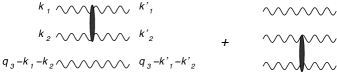
Based upon the results obained in this (and previous) papers, a few general statemants can be made about higher order amplitudes. First, for the appearance of Regge cuts with reggeized gluons we need the process (Fig.20).

.
This contribution is expected to show up in the kinematic region where the energy of the produced particles have alternating signs (Fig.21).
.
For a Regge cut composed of n reggeized gluons the leading order BFKL kernel will have the form:
| (201) |
with . As indicated in Fig.LABEL:fig:double-disc(1)b, beyond leading order there will be interactions between more than two reggeized gluons Bartels:2012sw .
Second, starting with we expect to have multiple products of Regge cuts. For example, for we expect the triple product of the shortest cut (Fig.22)

.
It will be interesting to see
whether these products are consistent with exponentiation.
Acknowledgments:
I wish to express my deep gratitude to Lev Nikolaevich Lipatov who initiated this paper and provided substantial contributions. I also thank A.Kormilitzin for his valuable help. For valuable discussions I want to thank T.Bargheer, G.Papathanasiou, and A.Sabio Vera.
Appendix A BDS phases of the amplitude
As explained in Bartels:2013jna for the amplitude, there are phase factors related to Regge pole terms and to the functions contained in the BDS amplitude (27). Their derivation has been described in detail in Bartels:2013jna , and in the following we present a list for those different kinematic regions of the amplitude which contain Regge cuts. We list the phases and using the notation of Bartels:2013jna :
Appendix B Trigonometric factors for the amplitude
B.1 Regge pole contributions
In this appendix we list the trigonometric prefactors for the Regge pole contributions. The Regge poles contribute to all 42 partial waves. We present the different groups.
B.1.1 Five singlets: LLLL,RRLL,RRRR,RRRL,RLLL
| (203) |
B.1.2 Three doublets: LRLL, RLRL, RRLR
| (204) |
and
| (205) |
and
| (206) |
B.1.3 Four triplets: LLRL, LRRL, RLLR, RLRR
| (207) |
| (208) |
| (209) |
| (210) |
B.1.4 Two quartets: LLLR, LRRR
| (211) |
| (212) |
B.1.5 A quintet: LRLR
| (213) |
B.1.6 A sextet: LLRR
| (214) |
B.2 Regge cut contributions
In the following we list the trigonometric factors of Regge cut contributions in the partial waves. Let us begin with a general remark. When making an ansatz for a Regge cut contribution, we initially should allow for independent contributions in each partial wave. As an example (see eq.(C.1) below), the contribution of the Regge cut in inside could be different from the one inside , i.e. our ansatz should allow for . However, from the requirement that in the region of positive energies this cut contribution must cancel in the sum of the two partial waves we conclude that the two Regge cut functions must be equal: . In the following we will make repeated use of this argument to simplify our discussion. For simplicity we use un-primed variables; when inserting the Regge cut terms into the integral (22) we have to switch to the primed variables .
B.2.1 Short Regge cut in the channel
The short Regge cut in the channel contributes to the doublet , to the triplet , to the quartet , and to the quintet . The results are:
| (215) | |||||
| (216) | |||||
| (217) | |||||
| (218) |
B.2.2 Short Regge cut in the channel
The short Regge cut in the channel appears in the doublet , the two triplets and , and in the sixtet . One finds:
| (219) | |||||
| (220) | |||||
| (221) | |||||
| (222) |
B.2.3 Long Regge cut in the and channels
This cut appears in the triplets and , in the quartet , and in the sextet . The form of the partial waves is the following:
| (223) |
| (224) |
| (225) |
| (226) |
B.2.4 Regge cuts in the and in the channels
This contribution appears in the quintet: .
| (227) |
B.2.5 Very long Regge cut in the , , and channels
This cut contributes to partial waves of the two quartets: , , of the quintet: , and of the sixtet . They have the following form:
| (228) |
| (229) |
| (230) |
| (231) |
B.2.6 The Regge cut consisting of 3 reggeized gluons
This cut contributes to four partial waves of the sixtet, . They have the following form:
| (232) |
Appendix C Regge pole contributions in different kinematic regions
| (free term) | |
|---|---|
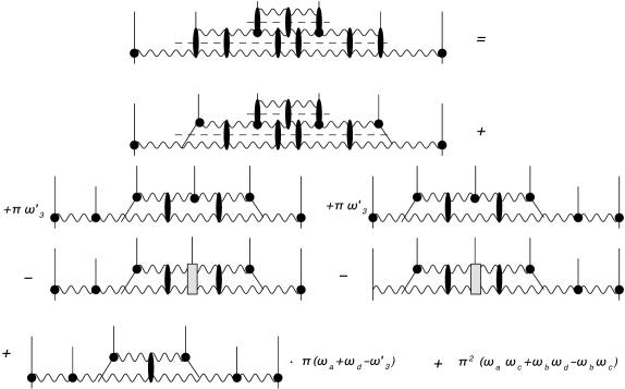
Appendix D Singular pieces of the long cut, the very long cut, the double cut, and the 3-reggeon cut
In this section we adopt a slightly different way of our discussion. Namely, we return to the starting point (22) which we write in the form (73) and focus on the last line: phase -dependent partial wave. This implies that, for -channels without a Regge cut, we have a pole factor which, for simplicity, we will not write. The and channels are always free from Regge cuts, therefore we do not need to introduce and . At the end of the discussion, when we will carry out the integrations: for -channels with a Regge pole only we have , whereas for -channels with a Regge cut we perform the shift . This provides that, for each channel, we have the Regge pole factor which is part of the BDS part. The same procedure will also be applied for energy discontinuities.
D.1 The long cut
This long cut has already been studied for the amplitude, and we can simply recapitulate the discussion Bartels:2013jna ; Bartels:2014jya and apply to the long cut in the and channels. The equations for the long -Regge cut are:
| (233) | |||||
| (234) | |||||
| (235) | |||||
When combining with Regge pole terms it was found in Bartels:2013jna that we should start from the last kinematic region, , in which the most singular piece of the Regge pole contribution has the simple form
| (237) |
Together with the singular pieces in (D.1) the sum of all singular terms which have to be compensated by the becomes
| (238) | |||||
with
| (239) | |||||
| (240) |
Since all partial waves etc. are real-valued, we are also searching for we real-valued corrections ; together with the complex conjugate of (238)
| (241) |
we thus have two equations which allow to find and :
| (242) |
or, in more detail:
Here all subtraction terms are free from Regge cut pieces, i.e.proportional to Regge pole factors. Therefore the -integrations simply imply , . Similar subtractions apply to the long - cut.The complete list of finite results is given in section 4.2.
D.2 The very long cut, the double cut, and the 3-reggeon cut
D.2.1 The very long cut for the regions , , ,
We begin with the very long cut in the region . Looking at the singularities of the Regge pole terms in Appendix B, we recognize that the region may play the same role as the region above has been playing for the long cut: in this region the Regge pole singularity is of the form
| (244) |
Beginning with (122) and disregarding, for the moment, the double cut we make the following ansatz for :
| (245) | |||
When combining this with the Regge pole of the region we obtain the conformal invariant Regge pole written in (131).
However, there is still the double cut piece, , which introduces additonal singularities. So the singular terms we have to cancel are
| (247) |
where depends upon and , As shown in section 6.2, factorizes:
| (248) | |||||
with
| (249) |
We write the brackets in (247) as
| (250) |
where the real part is
| (251) |
and the imaginary part can be written as
| (252) |
with
| (253) |
We thus need to cancel the singular terms , and arrive at the subtraction , instead of (245):
Here we observe that, in contrast to all previous subtractions, now being a subtraction to the three dimensional integral contains also integrals: in and in , . For later purposes it is sometimes convenient to write as
D.2.2 The very long cut for the regions , ,
For the regions (126) and (127) we have to modify the ansatz. Addition of the last term of (126) leads, in (D.2.1), to the change :
| (257) | |||||
and the cancellation of singularities proceeds in the same way as before. The same arguments appliy to the region in (127):
| (258) | |||||
The three equations for , and , together with (which is the complex conjugate of ) can be used to find the expressions for etc:
| (259) | |||
| (260) | |||
| (261) | |||
| (262) | |||
Making use of the relations:
| (263) |
and
| (264) |
we can also write:
| (265) | |||
| (266) | |||
| (267) | |||
| (268) |
We should stress that the subtractions of the partial waves etc. are all real-valued, as it should be.
D.2.3 The very long cut for the regions , ,
For the remaining kinematic regions and we first need to analyse the first two lines of (128) and (6.1), then find the subtraction of the three reggeon cut contribution, . We beginn with the the first two lines of (128), disregarding for the moment the double cut term . First we notice that the simple ansatz
| (269) | |||
removes the singular terms. Here the first term compensates the most singular piece of the Regge pole; it has the same form as in the region . On the other hand, our subtraction must be consistent with the complex complex conjugate of the Regge cut subtractions of in (245). We therefore write
| (270) |
The last three lines can be written in the more compact form
| (271) |
with
| (272) |
Next we include the double cut. Repeating our discussion given in the context of the region , we replace the first term in (269) by , and the first 2 lines inside the square brackets become:
| (273) | |||
Next we turn to the two last lines of (128) and collect the singular pieces which need to be compensated. First, in the third line we decompose the second and third terms:
| (274) |
The real part together with the last line of (128) suggests to define
| (275) |
In (128) the sum of these terms then becomes:
| (276) |
Here the first line contains the singular terms which have to be compensated. Using our result for the sum of the singular terms can be written as:
| (277) |
Now we combine (D.2.3) with the last line of (273). We notice that the second term in the last line of (273) cancels part of the second part of (D.2.3). Using the identity
| (278) |
we are left with:
| (279) |
Defining the subtraction
| (280) |
we finally arrive at:
| (281) |
Finally the region . Starting from (6.1) we proceed in the same way. Addressing the first two lines (ignoring for the moment ) we observe that the ansatz
| (282) | |||
after combination with the Regge singular pole term removes the singular terms. Here the second line is the complex conjugate of the second line of (269). The analogue of (271), after some algebra, has the form
Including next the double cut term , the singularities add up to
| (284) |
Adding the last two lines of (6.1) the first part is modifiied:
| (285) |
In (282) we therefore replace the first term by . In analogy with (273) we then have
| (286) | |||
Turning to the 3rd and 4th line of (6.1) we find, in analogy with (D.2.3),
| (287) |
Combining with the last line of (286) we finally have:
| (288) |
D.2.4 The discontinuity
We complete this section by inserting the subtractions into the discontinuities and and demonstrating the cancellation of the singularities.. We return to the rhs of (7.1) and undo the -integrations. We then insert the subtractions derived in the previous subsections. To show the cancellation of all singular terms requires some algebra, and we only scetch the main steps. For the first three lines (without the double cut term, ) we have the subtractions listed in (D.2.2) - (D.2.2). We combine the last term of the third line, , with the first term of the product in the next line and with the two terms in the 7th line. Using our previous notation we arrive at:
| (289) | |||||
In a similar way we rewrite the curley bracket in the 5th line and obtain:
| (290) |
Our expression for the discontinuity thus takes the somewhat modified form:
Now we are ready to verify the cancellation of the different singularities. All subtractions etc. have singulartities due to the denominatoirs . After some algebra one finds that in the sum of the first two lines of (D.2.4) these singulartities cancel completely.
Next we collect the terms proportional to , and ; they contain short cut contributions, or , multiplied by a singular pole term. They are contained in the first two lines of (D.2.4) (in the etc.), in the 5th line, and in . With the identity (D.2.1) the sum of terms proportional to , and becomes
| (292) |
Next we collect terms proportional to . They are contained in and , in in the 7th line, and in the 8th line of of (D.2.4). For the sum of all and the coefficients are :
| (293) |
and
| (294) |
Making use of our results for and and adding the last line of (D.2.4) we find for the sum:
| (295) | |||
Similar results hold for and . As expected, all double poles cancel.
Finally we collect terms proportional to simple poles contained in , , and . For the sum of terms containing we obtain:
| (297) |
For the sum of terms proportional to we find:
| (298) |
This completes our proof that, after inserting all the subtractions and performing the -integrations, we end up with a finite expression for the single discointinuity , as written in (7.1).
D.2.5 The double discontinuity
We start from (7.2.2). As the first step, using (280), we subsitute
| (299) |
and combine with the folllowing three lines. We obtain:
As a result, all singular terms have been cancelled, except for the Regge pole term in the last line. Next we use the decomposition of the Regge cut amplitudes etc and obtain for the regular pieces (disregarding the overall phase factor )
| (301) |
Collecting the remaining singular terms, we use
| (302) | |||||
and
Here the last line belongs to the regular pieces, i.e. has to be part of (D.2.5). For the sum of all remaining terms we first collect all singular terms (proportional to , , ), together with the the last line:
| (304) |
Next we insert:
| (305) | |||||
| (306) |
and obtain
| (308) |
Finally we use
| (309) |
and find complete cancellation of all singular terms:
| eq(D.2.5) | ||||
The final sum, after perfoming the -integrations, is given in (7.2.2).
References
- (1) Z. Bern, L. J. Dixon and V. A. Smirnov, Phys. Rev. D 72 (2005) 085001 [hep-th/0505205].
- (2) J. Bartels, L. N. Lipatov and A. Sabio Vera, Phys. Rev. D 80 (2009) 045002 [arXiv:0802.2065 [hep-th]].
- (3) J. Bartels, L. N. Lipatov and A. Sabio Vera, Eur. Phys. J. C 65 (2010) 587 [arXiv:0807.0894 [hep-th]].
- (4) J. Bartels, A. Kormilitzin and L. Lipatov, Phys. Rev. D 89 (2014) 065002 [arXiv:1311.2061 [hep-th]].
- (5) J. Bartels, A. Kormilitzin and L. N. Lipatov, Phys. Rev. D 91 (2015) 045005 [arXiv:1411.2294 [hep-th]].
- (6) A. B. Goncharov, M. Spradlin, C. Vergu and A. Volovich, Phys. Rev. Lett. 105 (2010) 151605 [arXiv:1006.5703 [hep-th]].
- (7) L. N. Lipatov and A. Prygarin, Phys. Rev. D 83 (2011) 125001 doi:10.1103/PhysRevD.83.125001 [arXiv:1011.2673 [hep-th]].
- (8) J. Bartels, L. N. Lipatov and A. Prygarin, Phys. Lett. B 705 (2011) 507 doi:10.1016/j.physletb.2011.09.061 [arXiv:1012.3178 [hep-th]].
- (9) V. Del Duca, C. Duhr and V. A. Smirnov, “An Analytic Result for the Two-Loop Hexagon Wilson Loop in N = 4 SYM,” JHEP 1003 (2010) 099 [arXiv:0911.5332 [hep-ph]].
- (10) V. Del Duca, C. Duhr and V. A. Smirnov, JHEP 1005 (2010) 084 [arXiv:1003.1702 [hep-th]].
- (11) L. J. Dixon, J. M. Drummond and J. M. Henn, “Bootstrapping the three-loop hexagon,” JHEP 1111 (2011) 023 [arXiv:1108.4461 [hep-th]].
- (12) L. J. Dixon, J. M. Drummond and J. M. Henn, JHEP 1201 (2012) 024 [arXiv:1111.1704 [hep-th]].
- (13) L. J. Dixon, C. Duhr and J. Pennington, JHEP 1210 (2012) 074 [arXiv:1207.0186 [hep-th]].
- (14) J. Pennington, JHEP 1301 (2013) 059 [arXiv:1209.5357 [hep-th]].
- (15) L. J. Dixon, J. M. Drummond, M. von Hippel and J. Pennington, JHEP 1312 (2013) 049 doi:10.1007/JHEP12(2013)049 [arXiv:1308.2276 [hep-th]].
- (16) T. Bargheer, G. Papathanasiou and V. Schomerus, JHEP 1605 (2016) 012 doi:10.1007/JHEP05(2016)012 [arXiv:1512.07620 [hep-th]].
- (17) V. Del Duca, S. Druc, J. Drummond, C. Duhr, F. Dulat, R. Marzucca, G. Papathanasiou and B. Verbeek, JHEP 1806 (2018) 116 doi:10.1007/JHEP06(2018)116 [arXiv:1801.10605 [hep-th]].
- (18) V. Del Duca, C. Duhr, F. Dulat and B. Penante, JHEP 1901 (2019) 162 doi:10.1007/JHEP01(2019)162 [arXiv:1811.10398 [hep-th]].
- (19) S. Caron-Huot, L. J. Dixon, F. Dulat, M. von Hippel, A. J. McLeod and G. Papathanasiou, JHEP 1908 (2019) 016 doi:10.1007/JHEP08(2019)016 [arXiv:1903.10890 [hep-th]].
- (20) T. Bargheer, V. Chestnov and V. Schomerus, arXiv:1906.00990 [hep-th].
- (21) V. Del Duca, S. Druc, J. M. Drummond, C. Duhr, F. Dulat, R. Marzucca, G. Papathanasiou and B. Verbeek, arXiv:1912.00188 [hep-th].
- (22) L. N. Lipatov, J. Phys. A 42 (2009) 304020 [arXiv:0902.1444 [hep-th]].
- (23) L. N. Lipatov, Theor. Math. Phys. 170 (2012) 166 [arXiv:1008.1015 [hep-th]].
- (24) J.Bartels and T.Bargheer, in preparation
- (25) J. Bartels, V. S. Fadin, L. N. Lipatov and G. P. Vacca, Nucl. Phys. B 867 (2013) 827 doi:10.1016/j.nuclphysb.2012.10.024 [arXiv:1210.0797 [hep-ph]].