Entropy conservation property and entropy stabilization of high-order continuous Galerkin approximations to scalar conservation laws

Abstract

This paper addresses the design of linear and nonlinear stabilization procedures for high-order continuous Galerkin (CG) finite element discretizations of scalar conservation laws. We prove that the standard CG method is entropy conservative for the square entropy. In general, the rate of entropy production/dissipation depends on the residual of the governing equation and on the accuracy of the finite element approximation to the entropy variable. The inclusion of linear high-order stabilization generates an additional source/sink in the entropy budget equation. To balance the amount of entropy production in each cell, we construct entropy-dissipative element contributions using a coercive bilinear form and a parameter-free entropy viscosity coefficient. The entropy stabilization term is high-order consistent, and optimal convergence behavior is achieved in practice. To enforce preservation of local bounds in addition to entropy stability, we use the Bernstein basis representation of the finite element solution and a new subcell flux limiting procedure. The underlying inequality constraints ensure the validity of localized entropy conditions and local maximum principles. The benefits of the proposed modifications are illustrated by numerical results for linear and nonlinear test problems.

1 Introduction

The design of property-preserving continuous Galerkin (CG) methods for hyperbolic conservation laws is particularly difficult in the context of high-order finite element approximations. Even linear advection problems with smooth exact solutions require the use of high-order stabilization to achieve optimal convergence rates with CG approximations on general meshes [30]. In the nonlinear case, a well-designed numerical scheme should be entropy stable [1, 8, 33]. A failure to satisfy this requirement may cause convergence to a wrong weak solution. Tadmor’s entropy stability theory [32, 33] provides a general framework for designing numerical fluxes that satisfy cell entropy inequalities. Positivity preservation and local maximum principles can be enforced using flux or slope limiting techniques [8, 22, 26]. Many high-resolution finite volume or discontinuous Galerkin (DG) methods are designed in this way. Unfortunately, direct manipulation of numerical fluxes and/or solution gradients is not an option for high-order continuous finite element approximations. However, the desired properties can be achieved using the framework of algebraic flux correction (AFC) for linear transport equations [5, 24] and its recent extensions to nonlinear hyperbolic conservation laws [13, 16, 25, 27].

An entropy stable and locally bound-preserving AFC scheme for continuous linear ($\mathbb{P}_{1}$) and multilinear ($\mathbb{Q}_{1}$) finite elements was designed in [28] using graph Laplacian stabilization and a monolithic limiting strategy. Alternative approaches to enforcing entropy stability in finite element schemes include the use of residual-based entropy viscosity [13, 16] and Rusanov-type penalization for the gradients of entropy variables [1, 2, 26]. In the present paper, we extend the entropy correction tools proposed in [1, 26, 28] to stabilized high-order CG approximations and combine them with the subcell flux limiting strategy developed in [27] for AFC schemes based on high-order Bernstein finite elements. Moreover, we prove that the standard CG method is entropy conservative for the square entropy. In contrast to the square entropy stability property of DG methods for scalar conservation laws [19], this result seems to be largely unknown. The use of a general entropy and/or inclusion of linear high-order stabilization terms produces additional sources or sinks in the entropy balance equation associated with the semi-discrete CG scheme. To convert this equation into a discrete entropy inequality, we add a nonlinear entropy dissipation term which represents a generalized high-order version of Abgrall’s [1] entropy fix. In the process of subcell flux correction, we blend the resulting entropy stable high-order scheme and a low-order compact-stencil approximation of Rusanov (local Lax-Friedrichs) type in a manner which guarantees the validity of all relevant constraints (conservation principles, entropy inequalities, maximum principles). Numerical studies are performed for linear and nonlinear test problems.

2 Entropy conservation property of the CG method

Let $u(\mathbf{x},t)$ be a scalar conserved quantity depending on the space location $\mathbf{x}\in\mathbb{R}^{d},\ d\in\{1,2,3\}$ and time instant $t\geq 0$. Consider an initial value problem of the form

$$\frac{\partial u}{\partial t}+\nabla\cdot\mathbf{f}(u)=0 \qquad\mbox{in}\ \mathbb{R}^{d}\times\mathbb{R}_{+},$$ (1a)

$$u(\cdot,0)=u_{0} \qquad\mbox{in}\ \mathbb{R}^{d},$$ (1b)

where $\mathbf{f}=(\mathsf{f}_{1},\ldots,\mathsf{f}_{d})$ is a possibly nonlinear flux function and $u_{0}:\mathbb{R}^{d}\to\mathcal{G}$ is the data of the initial condition. A convex set $\mathcal{G}\subset\mathbb{R}$ is called an invariant set of problem (1a)–(1b) if the exact solution $u$ stays in $\mathcal{G}$ for all $t>0$ [15]. A convex function $\eta:\mathcal{G}\to\mathbb{R}$ is called an entropy and $v(u)=\eta^{\prime}(u)$ is called an entropy variable if there exists an entropy flux $\mathbf{q}:\mathcal{G}\to\mathbb{R}^{d}$ such that $v(u)\mathbf{f}^{\prime}(u)=\mathbf{q}^{\prime}(u)$. A weak solution $u$ of (1a) is called an entropy solution if the entropy inequality

$$\frac{\partial\eta}{\partial t}+\nabla\cdot\mathbf{q}(u)\leq 0\qquad\mbox{in}\ \mathbb{R}^{d}\times\mathbb{R}^{+}$$ (2)

holds for any entropy pair $(\eta,\mathbf{q})$. For any smooth weak solution, the conservation law

$$\frac{\partial\eta}{\partial t}+\nabla\cdot\mathbf{q}(u)=0\qquad\mbox{in}\ \mathbb{R}^{d}\times\mathbb{R}^{+}$$ (3)

can be derived from (1a) using multiplication by the entropy variable $v$, the chain rule, and the definition of an entropy pair. Hence, entropy is conserved in smooth regions and dissipated at shocks.

Adopting the terminology of Guermond et al. [13, 15], we will call a numerical scheme invariant domain preserving (IDP) if the solution of the (semi-)discrete problem is guaranteed to stay in an invariant set $\mathcal{G}$. Additionally, a property-preserving discretization of (1a) should be entropy stable, i.e., it should satisfy a discrete version of the entropy inequality (2). The lack of entropy stability is a typical reason for convergence of numerical schemes to nonphysical weak solutions.

To discretize (1a) in a bounded domain $\Omega\subset\mathbb{R}^{d}$, we use the continuous Galerkin (CG) method and a conforming mesh $\mathcal{T}_{h}=\{K^{1},\ldots,K^{E_{h}}\}$. For simplicity, we assume that the imposed boundary conditions are periodic. Let $V_{h}^{e}\in\{\mathbb{P}_{p}(K^{e}),\mathbb{Q}_{p}(K^{e})\},\ p\in\mathbb{N}$ denote the polynomial space of the finite element approximation on $K^{e},\ e=1,\ldots,E_{h}$ and $V_{h}=\{v_{h}\in C(\bar{\Omega}_{h})\,:\,v_{h}|_{K^{e}}\in V_{h}^{e},\ e=1,\ldots,E_{h}\}$ the space of continuous piecewise-polynomial functions defined on $\bar{\Omega}_{h}=\bigcup_{i=1}^{E_{h}}K^{e}$. Each function $v_{h}\in V_{h}$ can be written as $v_{h}=\sum_{j=1}^{N_{h}}v_{j}\varphi_{j}$, where $\varphi_{1},\ldots,\varphi_{N_{h}}$ are Lagrange or Bernstein basis functions associated with nodal points $\mathbf{x}_{1},\ldots,\mathbf{x}_{N_{h}}\in\bar{\Omega}_{h}$. We define the full stencil of node $i$ as the integer set $\mathcal{N}_{i}=\bigcup_{e\in\mathcal{E}_{i}}\mathcal{N}^{e}$, where $\mathcal{E}_{i}$ denotes the set of (numbers of) elements containing the point $\mathbf{x}_{i}$ and $\mathcal{N}^{e}$ is the set of (numbers of) nodes belonging to $K^{e}$. In addition to full stencils, we will use compact nearest-neighbor stencils in the description of the proposed methods below.

Approximating the exact entropy solution $u$ of (1a) by $u_{h}\in V_{h}$, we consider the CG discretization

$$\sum_{e=1}^{E_{h}}\int_{K^{e}}w_{h}\left(\frac{\partial u_{h}}{\partial t}+\nabla\cdot\mathbf{f}(u_{h})\right)\,{\rm d}{\mathbf{x}}=0\qquad\forall w_{h}\in V_{h}.$$ (4)

Non-periodic flux boundary conditions can be taken into account by adding an integral over the inflow boundary of the computational domain $\Omega_{h}$, see [25, 27] for details.

Theorem 1 (Entropy behavior of the continuous Galerkin method).

Let $\{\eta(u),\mathbf{q}(u)\}$ be an entropy pair and $v(u)=\eta^{\prime}(u)$ the corresponding entropy variable. Suppose that (4) holds for $u_{h}\in V_{h}$. Then

$$\sum_{e=1}^{E_{h}}\int_{K^{e}}\left(\frac{\partial\eta(u_{h})}{\partial t}+\nabla\cdot\mathbf{q}(u_{h})\right)\,{\rm d}{\mathbf{x}}=\sum_{e=1}^{E_{h}}\int_{K^{e}}(v(u_{h})-v_{h})\left(\frac{\partial u_{h}}{\partial t}+\nabla\cdot\mathbf{f}(u_{h})\right)\,{\rm d}{\mathbf{x}}\quad\forall v_{h}\in V_{h}.$$ (5)

In particular, $\eta(u_{h})$ satisfies (5) for $v_{h}\equiv 0$ and for an arbitrary approximation $v_{h}\in V_{h}$ to $v(u_{h})$.

Proof 1.

Using the chain rule to differentiate $\eta(u)$, substituting $v(u_{h})$ for $\eta^{\prime}(u_{h})$ and recalling that $v(u_{h})\mathbf{f}^{\prime}(u_{h})=\mathbf{q}^{\prime}(u_{h})$ by definition of the entropy flux, we transform the left-hand side of (5) as follows:

$$\sum_{e=1}^{E_{h}}\int_{K^{e}}\left(\frac{\partial\eta(u_{h})}{\partial t}+\nabla\cdot\mathbf{q}(u_{h})\right)\,{\rm d}{\mathbf{x}} =\sum_{e=1}^{E_{h}}\int_{K^{e}}\left(v(u_{h})\frac{\partial u_{h}}{\partial t}+\mathbf{q}^{\prime}(u_{h})\cdot\nabla u_{h}\right)\,{\rm d}{\mathbf{x}}$$

$$=\sum_{e=1}^{E_{h}}\int_{K^{e}}v(u_{h})\left(\frac{\partial u_{h}}{\partial t}+\mathbf{f}^{\prime}(u_{h})\cdot\nabla u_{h}\right)\,{\rm d}{\mathbf{x}}$$

$$=\sum_{e=1}^{E_{h}}\int_{K^{e}}v(u_{h})\left(\frac{\partial u_{h}}{\partial t}+\nabla\cdot\mathbf{f}(u_{h})\right)\,{\rm d}{\mathbf{x}}.$$

The validity of representation (5) follows from the fact that (4) holds for any $v_{h}\in V_{h}$. $\Box$

Theorem 1 reveals that the CG method is globally entropy conservative in the following sense.

Corollary 1 (Entropy conservation property of the continuous Galerkin method).

For the square entropy $\eta(u)=\frac{u^{2}}{2}$, the CG approximation $u_{h}$ satisfies

$$\sum_{e=1}^{E_{h}}\int_{K^{e}}\left(\frac{\partial\eta(u_{h})}{\partial t}+\nabla\cdot\mathbf{q}(u_{h})\right)\,{\rm d}{\mathbf{x}}=0.$$ (6)

Proof 2.

The entropy variable associated with $u_{h}\in V_{h}$ is $v(u_{h})=u_{h}$. Hence, the right-hand side of the entropy balance equation (5) vanishes for the CG solution $u_{h}$ defined by (4).

Remark 1.

The rate of net entropy production for $\eta(u)\neq\frac{u^{2}}{2}$ is given by the weighted residual

$$\sum_{e=1}^{E_{h}}\int_{K^{e}}v(u_{h})\left(\frac{\partial u_{h}}{\partial t}+\nabla\cdot\mathbf{f}(u_{h})\right)\,{\rm d}{\mathbf{x}}.$$

A similar result was obtained by Jiang and Shu [19] in the context of DG methods.

3 Linear high-order stabilization

It is common knowledge that the convergence behavior of the CG method is unsatisfactory even for linear advection problems with smooth exact solutions. The provable order of accuracy w.r.t. the $L^{2}$ error is $O(h^{p})$, where $h$ is the mesh size and $p$ is the polynomial degree of the finite element approximation (see, e.g., Quarteroni and Valli [31], eq. (14.3.16)). To achieve optimal $O(h^{p+1/2})$ convergence rates on general meshes [7, 20], many stabilized CG methods of the form

$$\sum_{e=1}^{E_{h}}\left[\int_{K^{e}}w_{h}\left(\frac{\partial u_{h}}{\partial t}+\nabla\cdot\mathbf{f}(u_{h})\right)\,{\rm d}{\mathbf{x}}+s_{h}^{\text{LS},e}(w_{h},u_{h})\right]=0\qquad\forall w_{h}\in V_{h}$$ (7)

were proposed in the literature. The linear stabilization term $s_{h}^{\text{LS},e}(w_{h},u_{h})$ is usually defined as a weighted residual of the governing equation or of another relation which is satisfied for $h\to 0$.

The stabilization term of the streamline upwind Petrov-Galerkin (SUPG) method [6] is defined by

$$s_{h}^{\text{SUPG},e}(w_{h},u_{h})=\nu^{\text{SUPG},e}\int_{K^{e}}\left(\mathbf{f}^{\prime}(u_{h})\cdot\nabla w_{h}\right)\left(\dot{u}_{h}+\nabla\cdot\mathbf{f}(u_{h})\right)\,{\rm d}{\mathbf{x}},$$ (8)

where $\dot{u}_{h}\in V_{h}$ is an approximate time derivative and $\nu^{\text{SUPG},e}$ is a stabilization parameter depending on the local mesh size $h^{e}=|K^{e}|^{1/d}$. In the numerical experiments of Section 7, we use

$$\nu^{\text{SUPG},e}=\frac{\omega h^{e}}{2p\|\mathbf{f}^{\prime}(u_{h})\|_{L^{\infty}(K^{e})}},$$ (9)

where $\omega=1$ by default. Smaller values of $\omega$ can be used to adjust the amount of linear stabilization.

Existing theory [7, 20] guarantees $O(h^{p+1/2})$ convergence behavior of the consistent SUPG method for the linear advection equation provided that $\dot{u}_{h}$ is a sufficiently good approximation to $\frac{\partial u_{h}}{\partial t}$. The coefficients of $\dot{u}_{h}$ corresponding to (4) are given by the solution of the linear system

$$\sum_{e\in\mathcal{E}_{i}}\sum_{j\in\mathcal{N}^{e}}m_{ij}^{e}\dot{u}_{j}=-\sum_{e\in\mathcal{E}_{i}}\int_{K^{e}}\varphi_{i}\nabla\cdot\mathbf{f}(u_{h})\,{\rm d}{\mathbf{x}},\qquad i=1,\ldots,N_{h},$$ (10)

where we use the stencil notation introduced in Section 2. The coefficients $m_{ij}^{e}$ are defined by

$$m_{ij}^{e}=\int_{K^{e}}\varphi_{i}\varphi_{j}\,{\rm d}{\mathbf{x}}.$$ (11)

In contrast to other approximations of the time derivative, definition (10) supports the use of general time integrators and avoids the dependence of the parameter $\nu^{\text{SUPG},e}$ on the time step.

A closely related variational multiscale (VMS) method [21, 30] stabilizes (4) using the bilinear form

$$s_{h}^{\text{VMS},e}(w_{h},u_{h})=\nu^{\text{VMS},e}\int_{K^{e}}\nabla w_{h}\cdot(\nabla u_{h}-{\bf g}_{h})\,{\rm d}{\mathbf{x}},$$ (12)

where $\mathbf{g}_{h}=(\mathsf{g}_{h1},\ldots,\mathsf{g}_{hd})\in(V_{h})^{d}$ is a continuous approximation to the gradient $\nabla u_{h}$ and

$$\nu^{\text{VMS},e}=\frac{\omega h^{e}\|\mathbf{f}^{\prime}(u_{h})\|_{L^{\infty}(K^{e})}}{2p}.$$ (13)

Lohmann et al. [30] defined the continuous gradient $\mathbf{g}_{h}$ using the $L^{2}$ projection

$$\sum_{e=1}^{E_{h}}\int_{K^{e}}w_{h}({\bf g}_{h}-\nabla u_{h})\,{\rm d}{\mathbf{x}}=0\qquad\forall w_{h}\in V_{h}$$ (14)

which requires solution of $d$ linear systems with the consistent mass matrix

$$M_{C}=(m_{ij})_{i,j=1}^{N_{h}},\qquad m_{ij}=\sum_{e\in\mathcal{E}_{i}\cap\mathcal{E}_{j}}m_{ij}^{e}.$$ (15)

As shown in [30], the one-dimensional version of (12) using this definition of ${\bf g}_{h}$ is equivalent to the SUPG stabilization (8) for linear advection with constant velocity.

As an inexpensive alternative to gradient recovery via consistent-mass $L^{2}$ projections, we define

$${\bf g}_{h}=\sum_{j=1}^{N_{h}}{\bf g}_{j}\psi_{j}$$ (16)

using Lagrange basis functions $\psi_{1},\ldots,\psi_{N_{h}}$to interpolate the averaged nodal values

$${\bf g}_{i}=\frac{1}{m_{i}}\sum_{e\in\mathcal{E}_{i}}m_{i}^{e}\nabla u_{h}|_{K^{e}}({\bf x}_{i}),\qquad m_{i}=\sum_{e\in\mathcal{E}_{i}}m_{i}^{e},\qquad m_{i}^{e}=\int_{K^{e}}\varphi_{i}^{e}\,{\rm d}{\mathbf{x}}.$$ (17)

Note that both definitions of the reconstructed gradient produce ${\bf g}_{h}=\nabla u_{h}$ in the case $\nabla u_{h}\in(V_{h})^{d}$.

Remark 2.

If $u_{h}\in V_{h}$ is defined using the Lagrange basis as well, then $\varphi_{j}=\psi_{j}$ for $j=1,\ldots,N_{h}$. The limiting techniques presented in Section 4 require the use of Bernstein basis functions $\varphi_{j}\neq\psi_{j}$.

The ability of the above stabilization techniques to deliver the expected convergence rates for high-order finite element approximations to linear advection problems is verified in Section 7.

4 Nonlinear high-order stabilization

By virtue of Theorem 1, the entropy of the stabilized finite element approximation $u_{h}$ satisfies

$$\sum_{e=1}^{E_{h}}\int_{K^{e}}\left(\frac{\partial\eta(u_{h})}{\partial t}+\nabla\cdot\mathbf{q}(u_{h})\right)\,{\rm d}{\mathbf{x}}=\sum_{e=1}^{E_{h}}p^{e}_{h}(v_{h},u_{h}),$$ (18)

where $v_{h}=\sum_{j=1}^{N_{h}}v_{j}\varphi_{j}$ is defined in terms of $v_{j}=v(u_{j}),\ j=1,\ldots,N_{h}$ or as $L^{2}$ projection of $v(u_{h})$ into $V_{h}$. The bilinear form $p^{e}_{h}(v_{h},u_{h})$ of the local entropy production term is defined by

$$p^{e}_{h}(v_{h},u_{h})=\int_{K^{e}}(v(u_{h})-v_{h})\left(\frac{\partial u_{h}}{\partial t}+\nabla\cdot\mathbf{f}(u_{h})\right)\,{\rm d}{\mathbf{x}}-s_{h}^{\text{LS},e}(v_{h},u_{h}).$$ (19)

If we have $p^{e}_{h}(v_{h},u_{h})\leq 0$ for all $e=1,\ldots,E_{h}$, then the discrete entropy inequality

$$\sum_{e=1}^{E_{h}}\int_{K^{e}}\left(\frac{\partial\eta(u_{h})}{\partial t}+\nabla\cdot\mathbf{q}(u_{h})\right)\,{\rm d}{\mathbf{x}}\leq 0$$ (20)

holds for the solution $u_{h}$ of the semi-discrete problem (7). Ironically, the contribution of the linear stabilization term $s_{h}^{\text{LS},e}(v_{h},u_{h})$ may render $p^{e}_{h}(v_{h},u_{h})$ positive even in the case of the square entropy $\eta(u)=\frac{u^{2}}{2}$, in which $v(u_{h})=u_{h}$ and (20) holds as equality for the solution of (4). In other words, the use of (nonsymmetric) linear stabilization can cause or aggravate the lack of entropy stability.

To limit the amount of entropy production, we introduce an entropy viscosity (EV) term $s_{h}^{\text{EV},e}(w_{h},v_{h})$ such that $p^{e}_{h}(v_{h},u_{h})-s_{h}^{\text{EV},e}(v_{h},v_{h})\leq 0$ and, therefore, (20) holds for the solution $u_{h}$ of

$$\sum_{e=1}^{E_{h}}\left[\int_{K^{e}}w_{h}\left(\frac{\partial u_{h}}{\partial t}+\nabla\cdot\mathbf{f}(u_{h})\right)\,{\rm d}{\mathbf{x}}+s_{h}^{\text{LS},e}(w_{h},u_{h})+s_{h}^{\text{EV},e}(w_{h},v_{h})\right]=0\qquad\forall w_{h}\in V_{h}.$$ (21)

Entropy correction techniques of this kind trace their origins to the work of Abgrall [1]. As pointed out in [26], any symmetric positive definite (coercive) bilinear form $b^{e}(\cdot,\cdot)$ can be used to construct $s_{h}^{\text{EV},e}(w_{h},v_{h})$. Following [2, 28], we choose $b^{e}(\cdot,\cdot)$ to be the $L^{2}(K^{e})$ scalar product and define

$$s_{h}^{\text{EV},e}(w_{h},v_{h})=\nu^{\text{EV},e}\int_{K^{e}}(i_{h,1}^{e}w_{h}-i_{h,0}^{e}w_{h})(i_{h,1}^{e}v_{h}-i_{h,0}^{e}v_{h})\,{\rm d}{\mathbf{x}},$$ (22)

where $i_{h,1}^{e}v_{h}$ is the piecewise $\mathbb{P}_{1}/\mathbb{Q}_{1}$ Lagrange interpolant of the nodal values $\{v_{h}(\mathbf{x}_{j}),\ j\in\mathcal{N}^{e}\}$ and $i_{h,0}^{e}v_{h}$ is a piecewise-constant approximation defined by the subcell averages of $i_{h,1}^{e}v_{h}$, i.e., by averages over the elements of the submesh formed by the nodes $\{\mathbf{x}_{j},\ j\in\mathcal{N}^{e}\}$, cf. [27].

Remark 3.

The entropy stabilization term (22) and the entropy viscosity coefficient $\nu^{\text{EV},e}$ can also be constructed using $i_{h,1}^{e}v_{h}:=v_{h}$ and $i_{h,0}^{e}v_{h}:=\frac{1}{|K^{e}|}\int_{K^{e}}v_{h}\,{\rm d}{\mathbf{x}}$. This definition corresponds to the Rusanov dissipation employed in [2, 26]. The two versions are equivalent for $\mathbb{P}_{1}/\mathbb{Q}_{1}$ elements.

It remains to define the EV parameter $\nu^{\text{EV},e}\geq 0$. A lower bound $\nu^{\text{EV},e,\min}$ which guarantees entropy stability of the semi-discrete scheme (21) is provided by the following theorem.

Theorem 2 (Minimal entropy viscosity).

Let $p_{h}^{e}(v_{h},u_{h})$ be the local entropy production term defined by (19) and $\nu^{\text{\rm EV},e}$ an entropy viscosity coefficient which is bounded below by

$$\nu^{\text{\rm EV},e,\min}:=\frac{\max\{0,p_{h}^{e}(v_{h},u_{h})\}}{\int_{K^{e}}(i_{h,1}^{e}v_{h}-i_{h,0}^{e}v_{h})^{2}\,{\rm d}{\mathbf{x}}}.$$ (23)

Then the semi-discrete scheme defined by (21) and (22) satisfies the discrete entropy inequality (20).

Proof 3.

The assertion of the theorem is a direct consequence of the fact that the local entropy condition

$$p_{h}^{e}(v_{h},u_{h})-s_{h}^{\text{EV},e}(v_{h},v_{h})\leq 0$$ (24)

holds for $s_{h}^{\text{EV},e}(v_{h},v_{h})\geq\nu^{\text{\rm EV},e,\min}\int_{K^{e}}(i_{h,1}^{e}v_{h}-i_{h,0}^{e}v_{h})^{2}\,{\rm d}{\mathbf{x}}=\max\{0,p_{h}^{e}(v_{h},u_{h})\}.$ $\Box$

The use of $\nu^{\text{EV},e}=\nu^{\text{EV},e,\min}$ in (22) introduces the minimal amount of entropy stabilization which ensures the validity of the discrete entropy inequality (20). The corresponding semi-discrete scheme (21) is barely entropy stable (cf. [26, 28]) and may fail to converge to correct weak solutions. Adopting Tadmor’s design philosophy [32, 33], we adjust the levels of entropy dissipation by using a stabilization parameter $\nu^{\text{EV},e}\geq\nu^{\text{EV},e,\min}$ which depends on the local smoothness of the approximate solution.

Let $\pi^{e}_{h}:L^{2}(K^{e})\to\mathbb{P}_{p-1}(K^{e})$ denote the local $L^{2}$ projection operator into the polynomial space of degree $p-1\geq 0$. For any $u\in L^{2}(K^{e})$, the polynomial $\pi^{e}_{h}u\in\mathbb{P}_{p-1}(K^{e})$ is defined by

$$\int_{K^{e}}w_{h}^{e}(u-\pi^{e}_{h}u)\,{\rm d}{\mathbf{x}}=0\qquad\forall w_{h}^{e}\in\mathbb{P}_{p-1}(K^{e}).$$ (25)

To gain better control of local entropy production without losing high-order accuracy in smooth regions, we define the nonlinear stabilization term (22) using the entropy viscosity coefficient

$$\nu^{\text{EV},e}=\nu^{\text{EV},e,\min}+\frac{\left|\int_{K^{e}}\nabla v_{h}\cdot(\mathbf{f}(\pi^{e}_{h}u_{h})-\mathbf{f}(u_{h}))\,{\rm d}{\mathbf{x}}\right|}{\int_{K^{e}}(i_{h,1}^{e}v_{h}-i_{h,0}^{e}v_{h})^{2}\,{\rm d}{\mathbf{x}}}.$$ (26)

Remark 4.

In the unlikely case that $\nu^{\text{EV},e}$ defined by (26) becomes very large, explicit time discretizations of (21) may require the use of impractically small time steps. If implicit treatment of (22), as proposed in [26] in the context of DG-$\mathbb{P}_{1}$ approximations, is not an option, then an upper bound $\nu^{\text{EV},e,\max}$ may need to be imposed on the value of $\nu^{\text{EV},e}$. For $\nu^{\text{EV},e,\max}<\nu^{\text{EV},e,\min}$, condition (24) cannot be satisfied using (22) with $\nu^{\text{EV},e}\leq\nu^{\text{EV},e,\max}$. However, entropy stability is still guaranteed if (21) is constrained using the convex limiting techniques that we present in the next section.

5 Monolithic convex limiting

The stabilized high-order finite element scheme (21) may require additional modifications to ensure the invariant domain preservation (IDP) property and validity of local maximum principles for problems with discontinuities and propagating fronts. Bound-preserving convex limiting techniques for high-order Bernstein finite element approximations to scalar hyperbolic conservation laws were developed in [27] without taking entropy conditions into account. Entropy stability preserving (ESP) limiters were introduced in [26, 28] in the context of $\mathbb{P}_{1}/\mathbb{Q}_{1}$ approximations of CG and DG type. In this section, we generalize the convex limiting tools developed in [26, 27, 28] and apply them to (21).

Let $\varphi_{1},\ldots,\varphi_{N_{h}}$ be Bernstein basis functions spanning the finite element space $V_{h}$. The definition of these basis functions for simplex and tensor-product meshes can be found, e.g., in [30] and in the Appendix of [27]. The corresponding degrees of freedom $u_{1},\ldots,u_{N_{h}}$ are associated with the nodal points ${\bf x}_{1},\ldots,{\bf x}_{N_{h}}$ and called Bernstein coefficients. The approximate solution $u_{h}\in V_{h}$ satisfies [30]

$$\min_{j\in\mathcal{N}^{e}}u_{j}\leq u_{h}(\mathbf{x})=\sum_{j\in\mathcal{N}^{e}}u_{j}\varphi_{j}(\mathbf{x})\leq\max_{j\in\mathcal{N}^{e}}u_{j}\qquad\forall\mathbf{x}\in K^{e}.$$ (27)

Hence, the IDP property is guaranteed if all Bernstein coefficients of $u_{h}$ are in the admissible range.

Substituting test functions $w_{h}\in\{\varphi_{1},\ldots,\varphi_{N_{h}}\}$ into (21), we obtain a system of semi-discrete equations for the (generally time-dependent) Bernstein coefficients. This system is given by

$$\sum_{e\in\mathcal{E}_{i}}\sum_{j\in\mathcal{N}^{e}}m_{ij}^{e}\frac{\text{d}u_{j}}{\text{d}t}=-\sum_{e\in\mathcal{E}_{i}}\left[\int_{K^{e}}\varphi_{i}\nabla\cdot\mathbf{f}(u_{h})\,{\rm d}{\mathbf{x}}+s_{h}^{\text{LS},e}(\varphi_{i},u_{h})+s_{h}^{\text{EV},e}(\varphi_{i},v_{h})\right],\quad i=1,\ldots,N_{h}.$$ (28)

The coefficients $m_{ij}^{e}$ of the consistent element mass matrix $M_{C}^{e}=(m_{ij}^{e})_{i,j=1}^{N_{h}}$ are defined by (11).

In the process of monolithic convex limiting [25, 27], the element contributions to the residual of the high-order target scheme (28) are modified to guarantee the validity of property-preserving inequality constraints. For that purpose, we introduce the lumped element mass matrix $M_{L}^{e}=(\delta_{ij}m_{i}^{e})_{i,j=1}^{N_{h}}$, the element matrix $\mathbf{C}^{e}=(\mathbf{c}_{ij}^{e})_{i,j=1}^{N_{h}}$ of the discrete gradient operator, its ‘lumped’ counterpart $\tilde{\mathbf{C}}^{e}=M_{L}^{e}(M_{C}^{e})^{-1}\mathbf{C}^{e}$, and a discrete diffusion operator $\tilde{D}^{e}=(\tilde{d}_{ij}^{e})_{i,j=1}^{N_{h}}$. The diagonal entries $m_{i}^{e}=\sum_{j\in\mathcal{N}^{e}}m_{ij}^{e}$ of $M_{L}^{e}$ are the weights that we used in (17). They are positive since the Bernstein basis functions are nonnegative by definition. The vector-valued entries of $\mathbf{C}^{e}$ are given by

$$\mathbf{c}_{ij}^{e}=\int_{K^{e}}\varphi_{i}\nabla\varphi_{j}\,{\rm d}{\mathbf{x}}.$$ (29)

If node $i$ or node $j$ is an interior point of $\Omega_{h}$, integration by parts using Green’s formula yields

$$\sum_{e=1}^{E_{h}}\mathbf{c}_{ji}^{e}=-\sum_{e=1}^{E_{h}}\mathbf{c}_{ij}^{e}.$$ (30)

An analytical formula for the entries of $\tilde{\mathbf{C}}^{e}$ is derived in the Appendix of [27], where we show that this element matrix has the same compact sparsity pattern as the collocated piecewise $\mathbb{P}_{1}/\mathbb{Q}_{1}$ approximation on a subdivision of $K^{e}$ into subcells. That is, we have $\tilde{\mathbf{c}}_{ij}=0$ if nodes $i$ and $j$ are not nearest neighbors belonging to the same subcell. On meshes consisting of parallelograms or parallelepipeds, the entries $\tilde{\mathbf{c}}_{ij}$ associated with diagonal subcell neighbors vanish as well [18]. Therefore, the sparsity pattern of the element contribution $\tilde{\mathbf{C}}^{e}$ to the lumped discrete gradient is defined by tensor products of one-dimensional three-point stencils for $d$ coordinate directions. The element matrix $\tilde{D}^{e}$ of the discrete diffusion (alias graph Laplacian [13, 15]) operator has the same sparsity pattern as $\tilde{\mathbf{C}}^{e}$. Let $\tilde{\mathcal{N}}_{i}^{e}=\{j\in\mathcal{N}^{e}\,:\,|\tilde{\mathbf{c}}_{ij}^{e}|+|\tilde{\mathbf{c}}_{ji}^{e}|>0\}$ denote the compact element stencil of node $i\in\mathcal{N}^{e}$. By default, the artificial diffusion coefficients $\tilde{d}_{ij}^{e}$ are defined by the local Lax-Friedrichs (LLF) formula [15, 27, 28]

$$\tilde{d}_{ij}^{e}=\begin{cases}\max\{|\tilde{\mathbf{c}}_{ij}^{e}|\lambda_{ij}^{\max},|\tilde{\mathbf{c}}_{ji}^{e}|\lambda_{ji}^{\max}\}&\mbox{if}\ i\in\mathcal{N}^{e},\ j\in\tilde{\mathcal{N}_{i}^{e}}\backslash\{i\},\\ -\sum_{k\in{\tilde{\mathcal{N}}_{i}^{e}}\backslash\{i\}}\tilde{d}_{ik}^{e}&\mbox{if}\ j=i\in\mathcal{N}^{e},\\ 0&\mbox{otherwise},\end{cases}$$ (31)

where $\lambda_{ij}^{\max}$ is a guaranteed upper bound for the maximal wave speed [15, 28]

$$\lambda_{ij}^{\max}\geq\max_{\omega\in[0,1]}|\mathbf{n}_{ij}^{e}\cdot\mathbf{f}^{\prime}(\omega u_{i}+(1-\omega)u_{j})|,\qquad\mathbf{n}_{ij}^{e}=\frac{\tilde{\mathbf{c}}_{ij}^{e}}{|\tilde{\mathbf{c}}_{ij}^{e}|}.$$ (32)

The monolithic convex limiting approach developed in [25, 27, 28] approximates (28) by

$$\sum_{e\in\mathcal{E}_{i}}m_{i}^{e}\frac{\mathrm{d}u_{i}}{\mathrm{d}t}=\sum_{e\in\mathcal{E}_{i}}\sum_{j\in\tilde{\mathcal{N}}_{i}^{e}\backslash\{i\}}[\tilde{d}_{ij}^{e}(u_{j}-u_{i})+\bar{f}_{ij}^{e}-\tilde{\mathbf{c}}_{ij}^{e}\cdot(\mathbf{f}(u_{j})-\mathbf{f}(u_{i}))].$$ (33)

As shown in [15], the low-order LLF scheme corresponding to $\bar{f}_{ij}^{e}=0$ is locally bound-preserving and entropy stable for any convex entropy. If discretization in time is performed using a strong stability preserving (SSP) Runge-Kutta method [10], the forward Euler update corresponding to a single stage satisfies a discrete entropy inequality for any convex entropy $\eta(u)$ [15]. Moreover, a local discrete maximum principle holds for time steps satisfying a CFL-like time step restriction [15, 27].

The stabilized high-order approximation (28) can also be written in the compact-stencil form (33) using an array of antidiffusive subcell fluxes $\tilde{f}_{ij}^{e}$ which we derive here for the reader’s convenience. Let $\tilde{\varphi}_{1},\ldots,\tilde{\varphi}_{N_{h}}$ denote the basis functions of the subcell $\mathbb{P}_{1}/\mathbb{Q}_{1}$ approximation. Define [18]

$$\tilde{m}_{ij}^{e}=\begin{cases}\int_{K^{e}}\tilde{\varphi}_{i}\tilde{\varphi}_{j}\,{\rm d}{\mathbf{x}}&\mbox{if}\ i\in\mathcal{N}^{e},\ j\in\tilde{\mathcal{N}}_{i}^{e}\backslash\{i\},\\ -\sum_{k\in\tilde{\mathcal{N}}_{i}\backslash\{i\}}\tilde{m}_{ik}^{e}&\mbox{if}\ j=i\in\mathcal{N}^{e},\\ 0&\mbox{otherwise}.\end{cases}$$ (34)

The compact-stencil scheme (33) with subcell fluxes $\bar{f}_{ij}^{e}=\tilde{f}_{ij}^{e}$ is equivalent to (28) for

$$\tilde{f}_{ij}^{e}=\tilde{m}_{ij}^{e}(\dot{w}_{j}^{e}-\dot{w}_{i}^{e})+\tilde{d}_{ij}^{e}(u_{i}-u_{j}),\qquad\forall i\in\mathcal{N}^{e},\ j\in\tilde{\mathcal{N}}^{e}_{i}\backslash\{i\},$$ (35)

where $\dot{w}_{i}^{e},\ i\in\mathcal{N}^{e}$ are subcell flux potentials satisfying the small sparse linear system (cf. [27])

$$\sum_{j\in\tilde{\mathcal{N}}_{i}^{e}}\tilde{m}_{ij}^{e}\dot{w}_{j}^{e} =\sum_{j\in\mathcal{N}^{e}\backslash\{i\}}m_{ij}^{e}(\dot{u}_{i}^{S}-\dot{u}_{j}^{S})+\sum_{j\in\mathcal{N}^{e}}(\tilde{\mathbf{c}}_{ij}^{e}-\mathbf{c}_{ij}^{e})\cdot\mathbf{f}(u_{j})-\sum_{j\in\mathcal{N}^{e}}\mathbf{c}_{ji}^{e}\cdot\mathbf{f}(u_{j})$$

$$+\int_{K^{e}}\nabla\varphi_{i}\cdot\mathbf{f}(u_{h})\,{\rm d}{\mathbf{x}}-s_{h}^{\text{LS},e}(\varphi_{i},u_{h})-s_{h}^{\text{EV},e}(\varphi_{i},v_{h}),\qquad i\in\mathcal{N}^{e}.$$ (36)

The number of unknowns equals the number of nodes per element. The solution of (36) is determined up to a constant, whose value has no influence on the value of the flux $\tilde{f}_{ij}^{e}$ defined by (35). The Bernstein coefficients $\dot{u}_{j}^{S}$ of the stabilized approximate time derivatives are obtained by solving

$$\sum_{e\in\mathcal{E}_{i}}\sum_{j\in\mathcal{N}^{e}}m_{ij}^{e}\dot{u}_{j}^{S}=-\sum_{e\in\mathcal{E}_{i}}\left[\int_{K^{e}}\varphi_{i}\nabla\cdot\mathbf{f}(u_{h})\,{\rm d}{\mathbf{x}}+s_{h}^{\text{LS},e}(\varphi_{i},u_{h})+s_{h}^{\text{EV},e}(\varphi_{i},v_{h})\right],\quad i=1,\ldots,N_{h}.$$ (37)

The subcell flux limiter proposed in [27] constrains $\tilde{f}_{ij}^{e}$ in a manner which guarantees that the result $\bar{u}_{i}$ of each SSP Runge-Kutta stage is bounded by the input data $u_{j},\ j\in\mathcal{N}_{i}$ as follows:

$$\min_{j\in\mathcal{N}_{i}}u_{j}=:u_{i}^{\min}\leq\bar{u}_{i}\leq u_{i}^{\max}:=\max_{j\in\mathcal{N}_{i}}u_{j}.$$ (38)

A proof of the IDP property is based on the representation of $\bar{u}_{i}$ in terms of the bar states

$$\bar{u}_{ij}^{e}=\frac{u_{j}+u_{i}}{2}-\frac{\tilde{\mathbf{c}}_{ij}^{e}\cdot(\mathbf{f}(u_{j})-\mathbf{f}(u_{i}))}{2\tilde{d}_{ij}^{e}}\in[u_{i}^{\min},u_{i}^{\max}],\qquad\bar{u}_{ij}^{e,*}=\bar{u}_{ij}^{e}+\frac{\alpha_{ij}^{e}\tilde{f}_{ij}^{e,*}}{2\tilde{d}_{ij}^{e}}$$ (39)

such that $\bar{u}_{ij}^{e,*}\in[u_{i}^{\min},u_{i}^{\max}]$ for any $\alpha_{ij}^{e}\in[0,1]$ if the limited flux $\tilde{f}_{ij}^{e,*}$ is given by [25, 27]

$$\tilde{f}_{ij}^{e,*}=\begin{cases}\min\,\left\{\tilde{f}_{ij}^{e},2\tilde{d}_{ij}^{e}\min\,\{u_{i}^{\max}-\bar{u}_{ij}^{e},\bar{u}_{ji}^{e}-u_{j}^{\min}\}\right\}&\mbox{if}\ \tilde{f}_{ij}^{e}>0,\\[7.11317pt] \max\left\{\tilde{f}_{ij}^{e},2\tilde{d}_{ij}^{e}\max\{u_{i}^{\min}-\bar{u}_{ij}^{e},\bar{u}_{ji}^{e}-u_{j}^{\max}\}\right\}&\mbox{otherwise}.\end{cases}$$ (40)

For further explanations and detailed proofs, we refer the interested reader to [25, 27, 28]. After the application of the IDP limiter, the magnitude of the bound-preserving flux $\tilde{f}_{ij}^{e,*}$ can be further reduced to enforce the following localized version of the entropy stability condition employed in [8, 28, 33].

Theorem 3 (Entropy correction via subcell flux limiting).

Let $\{\eta(u),\mathbf{q}(u)\}$ be an entropy pair and $v(u)=\eta^{\prime}(u)$ the corresponding entropy variable. Define $v_{h}=\sum_{j=1}^{N_{h}}v_{j}\varphi_{j}$ using the Bernstein coefficients $v_{j}=v(u_{j}),\ j=1,\ldots,N_{h}$. Suppose that the limited subcell fluxes $\bar{f}_{ij}^{e}$ satisfy

$$\frac{v_{i}-v_{j}}{2}[\tilde{d}_{ij}^{e}(u_{j}-u_{i})+\bar{f}_{ij}^{e}-\tilde{\mathbf{c}}_{ij}^{e}\cdot(\mathbf{f}(u_{j})+\mathbf{f}(u_{i}))]-\tilde{\mathbf{c}}_{ij}^{e}\cdot[\bm{\psi}(u_{j})-\bm{\psi}(u_{i})]\leq\tilde{p}_{ij}^{e},$$ (41)

where $\bm{\psi}(u)=v(u)\mathbf{f}(u)-\mathbf{q}(u)$ and

$$\sum_{i\in\mathcal{N}^{e}}\sum_{j\in\tilde{\mathcal{N}}^{e}_{i}\backslash\{i\}}\tilde{p}_{ij}^{e}\leq\sum_{i\in\mathcal{N}^{e}}\sum_{j\in\mathcal{N}^{e}\backslash\{i\}}(\tilde{\mathbf{c}}_{ij}^{e}-\mathbf{c}_{ij}^{e})\cdot\left[\left(\frac{v_{i}-v_{j}}{2}\right)(\mathbf{f}(u_{j})-\mathbf{f}(u_{i}))+{\bf q}(u_{j})-{\bf q}(u_{i})\right]=:p^{e,\max}.$$ (42)

Then the flux-corrected semi-discrete scheme (33) satisfies the discrete entropy inequality

$$\sum_{e=1}^{E_{h}}\sum_{i\in\mathcal{N}^{e}}m_{i}^{e}\frac{\mathrm{d}\eta(u_{i})}{\mathrm{d}t}\leq\sum_{e=1}^{E_{h}}\sum_{i\in\mathcal{N}^{e}}\sum_{j\in\mathcal{N}^{e}\backslash\{i\}}[G_{ij}^{e}-\mathbf{c}_{ij}^{e}\cdot(\mathbf{q}(u_{j})-\mathbf{q}(u_{i}))],$$ (43)

where

$$G_{ij}^{e}=\frac{v_{i}+v_{j}}{2}[\tilde{d}_{ij}^{e}(u_{j}-u_{i})+\bar{f}_{ij}^{e}]-\frac{v_{i}-v_{j}}{2}\,\mathbf{c}_{ij}^{e}\cdot(\mathbf{f}(u_{j})-\mathbf{f}(u_{i})).$$ (44)

Proof 4.

Using the chain rule to differentiate $\eta(u)$ and substituting $v_{i}$ for $\eta^{\prime}(u_{i})$, we obtain the identity

$$\sum_{e\in\mathcal{E}_{i}}m_{i}^{e}\frac{\mathrm{d}\eta(u_{i})}{\mathrm{d}t}=\sum_{e\in\mathcal{E}_{i}}m_{i}^{e}v_{i}\frac{\mathrm{d}u_{i}}{\mathrm{d}t}=\sum_{e\in\mathcal{E}_{i}}v_{i}\sum_{j\in\tilde{\mathcal{N}}_{i}^{e}\backslash\{i\}}[\tilde{g}_{ij}^{e}-\tilde{\mathbf{c}}_{ij}^{e}\cdot(\mathbf{f}(u_{j})-\mathbf{f}(u_{i}))],$$

where

$$\tilde{g}_{ij}^{e}=\tilde{d}_{ij}^{e}(u_{j}-u_{i})+\bar{f}_{ij}^{e}.$$

By definition, the entries $\tilde{\mathbf{c}}_{ij}^{e}$ of the element matrix $\tilde{\mathbf{C}}^{e}=M_{L}^{e}(M_{C}^{e})^{-1}\mathbf{C}^{e}$ satisfy the zero sum condition $\sum_{j\in\tilde{\mathcal{N}}_{i}^{e}}\tilde{\mathbf{c}}_{ij}^{e}=\mathbf{0}.$ Following the proof of Theorem 1 in [28], we use this zero sum property and the entropy stability condition (41) to estimate the rate of entropy production in element $K^{e}$ as follows:

$$v_{i}\sum_{j\in\tilde{\mathcal{N}}_{i}^{e}\backslash\{i\}}[\tilde{g}_{ij}^{e}-\tilde{\mathbf{c}}_{ij}^{e}\cdot(\mathbf{f}(u_{j})-\mathbf{f}(u_{i}))]=v_{i}\sum_{j\in\tilde{\mathcal{N}}_{i}^{e}\backslash\{i\}}[\tilde{g}_{ij}^{e}-\tilde{\mathbf{c}}_{ij}^{e}\cdot(\mathbf{f}(u_{j})+\mathbf{f}(u_{i}))]-2v_{i}\tilde{\mathbf{c}}_{ii}^{e}\cdot\mathbf{f}(u_{i})$$

$$=\sum_{j\in\tilde{\mathcal{N}}_{i}^{e}\backslash\{i\}}\left(\frac{v_{i}+v_{j}}{2}[\tilde{g}_{ij}^{e}-\tilde{\mathbf{c}}_{ij}^{e}\cdot(\mathbf{f}(u_{j})+\mathbf{f}(u_{i}))]+\frac{v_{i}-v_{j}}{2}[\tilde{g}_{ij}^{e}-\tilde{\mathbf{c}}_{ij}^{e}\cdot(\mathbf{f}(u_{j})+\mathbf{f}(u_{i}))]\right)-2v_{i}\tilde{\mathbf{c}}_{ii}^{e}\cdot\mathbf{f}(u_{i})$$

$$\leq\sum_{j\in\tilde{\mathcal{N}}_{i}^{e}\backslash\{i\}}\left(\frac{v_{i}+v_{j}}{2}[\tilde{g}_{ij}^{e}-\tilde{\mathbf{c}}_{ij}^{e}\cdot(\mathbf{f}(u_{j})+\mathbf{f}(u_{i}))]+\tilde{\mathbf{c}}_{ij}^{e}\cdot[\bm{\psi}(u_{j})-\bm{\psi}(u_{i})]+\tilde{p}_{ij}^{e}\right)-2v_{i}\tilde{\mathbf{c}}_{ii}^{e}\cdot\mathbf{f}(u_{i})$$

$$=\sum_{j\in\tilde{\mathcal{N}}_{i}^{e}\backslash\{i\}}\left(\frac{v_{i}+v_{j}}{2}[\tilde{g}_{ij}^{e}-\tilde{\mathbf{c}}_{ij}^{e}\cdot(\mathbf{f}(u_{j})+\mathbf{f}(u_{i}))]+\tilde{\mathbf{c}}_{ij}^{e}\cdot[\bm{\psi}(u_{j})+\bm{\psi}(u_{i})]+\tilde{p}_{ij}^{e}\right)-2\tilde{\mathbf{c}}_{ii}^{e}\cdot[v_{i}\mathbf{f}(u_{i})-\bm{\psi}(u_{i})]$$

$$=\sum_{j\in\tilde{\mathcal{N}}_{i}^{e}\backslash\{i\}}\left(\frac{v_{i}+v_{j}}{2}\tilde{g}_{ij}^{e}-\tilde{\mathbf{c}}_{ij}^{e}\cdot\left[\frac{v_{i}-v_{j}}{2}(\mathbf{f}(u_{j})-\mathbf{f}(u_{i}))+\mathbf{q}(u_{j})+\mathbf{q}(u_{i})\right]+\tilde{p}_{ij}^{e}\right)-2\tilde{\mathbf{c}}_{ii}^{e}\cdot\mathbf{q}(u_{i})$$

$$=\sum_{j\in\tilde{\mathcal{N}}_{i}^{e}\backslash\{i\}}\left(\frac{v_{i}+v_{j}}{2}\tilde{g}_{ij}^{e}-\tilde{\mathbf{c}}_{ij}^{e}\cdot\left[\frac{v_{i}-v_{j}}{2}(\mathbf{f}(u_{j})-\mathbf{f}(u_{i}))+\mathbf{q}(u_{j})-\mathbf{q}(u_{i})\right]+\tilde{p}_{ij}^{e}\right).$$

Summing over $e=1,\ldots,E_{h}$ and $i\in\mathcal{N}^{e}$, we use assumption (42) to eliminate the auxiliary quantities $\tilde{p}_{ij}^{e}$ and obtain $\mathbf{c}_{ij}^{e}$ instead of $\tilde{\mathbf{c}}_{ij}^{e}$ on the right-hand side of the final estimate

$$\sum_{e=1}^{E_{h}}\sum_{i\in\mathcal{N}^{e}}m_{i}^{e}\frac{\mathrm{d}\eta(u_{i})}{\mathrm{d}t} \leq\sum_{e=1}^{E_{h}}\sum_{i\in\mathcal{N}^{e}}\sum_{j\in\mathcal{N}^{e}\backslash\{i\}}\left(\frac{v_{i}+v_{j}}{2}\tilde{g}_{ij}^{e}-\mathbf{c}_{ij}^{e}\cdot\left[\frac{v_{i}-v_{j}}{2}(\mathbf{f}(u_{j})-\mathbf{f}(u_{i}))+\mathbf{q}(u_{j})-\mathbf{q}(u_{i})\right]\right)$$

$$=\sum_{e=1}^{E_{h}}\sum_{i\in\mathcal{N}^{e}}\sum_{j\in\mathcal{N}^{e}\backslash\{i\}}[G_{ij}^{e}-\mathbf{c}_{ij}^{e}\cdot(\mathbf{q}(u_{j})-\mathbf{q}(u_{i}))]$$

which proves the assertion of the theorem.    $\Box$

Remark 5.

In view of property (30), a further rearrangement yields the estimate (cf. [28])

$$\sum_{e=1}^{E_{h}}\sum_{i\in\mathcal{N}^{e}}m_{i}^{e}\frac{\mathrm{d}\eta(u_{i})}{\mathrm{d}t} \leq\sum_{i=1}^{N_{h}}\Big{(}\sum_{j\in\mathcal{N}_{i}\atop j>i}\frac{v_{i}+v_{j}}{2}\sum_{e\in\mathcal{E}_{i}\cap\mathcal{E}_{j}}\underbrace{(\tilde{g}_{ij}^{e}+\tilde{g}_{ji}^{e})}_{=0}-2\mathbf{q}(u_{i})\cdot\underbrace{\sum_{e\in\mathcal{E}_{i}}\mathbf{c}_{ii}^{e}}_{=\mathbf{0}}\Big{)}$$

$$-\sum_{i=1}^{N_{h}}\sum_{j\in\mathcal{N}_{i}\atop j>i}\left[\frac{v_{i}-v_{j}}{2}(\mathbf{f}(u_{j})-\mathbf{f}(u_{i}))+\mathbf{q}(u_{j})+\mathbf{q}(u_{i})\right]\cdot\underbrace{\sum_{e\in\mathcal{E}_{i}\cap\mathcal{E}_{j}}(\mathbf{c}_{ij}^{e}+\mathbf{c}_{ji}^{e})}_{=0}=0$$ (45)

in accordance with the fact that $\frac{\mathrm{d}}{\mathrm{d}t}\int_{\Omega}\eta(u)\,{\rm d}{\mathbf{x}}\leq 0$ under the assumption of periodic boundary conditions. Note that condition (30) and inequality (45) do not hold if the coefficients $\mathbf{c}_{ij}^{e}$ are replaced with the coefficients $\tilde{\mathbf{c}}_{ij}^{e}$ of the lumped discrete gradient. That is why we impose condition (42) and use it to obtain the final estimate in terms of $\mathbf{c}_{ij}^{e}$ rather than $\tilde{\mathbf{c}}_{ij}^{e}$ in the proof of Theorem 3.

For practical limiting purposes, we still need to define (i) distributed production bounds $\tilde{p}_{ij}^{e}$ such that assumption (42) holds and (ii) subcell fluxes $\bar{f}_{ij}^{e}$ such that the entropy stability condition (41) holds. The low-order LLF approximation corresponding to (33) with $\bar{f}_{ij}^{e}=0$ satisfies [8, 28]

$$\tilde{q}_{ij}^{e}:=\frac{v_{i}-v_{j}}{2}[\tilde{d}_{ij}^{e}(u_{j}-u_{i})-\tilde{\mathbf{c}}_{ij}^{e}\cdot(\mathbf{f}(u_{j})+\mathbf{f}(u_{i}))]-\tilde{\mathbf{c}}_{ij}^{e}\cdot[\bm{\psi}(u_{j})-\bm{\psi}(u_{i})]\leq 0.$$ (46)

To ensure that condition (41) holds for $\bar{f}_{ij}^{e}=0$ and, therefore, can be enforced by adjusting the magnitude of $\bar{f}_{ij}^{e}$, we must have $\tilde{q}_{ij}^{e}\leq\tilde{p}_{ij}^{e}$. If $p^{e,\max}\geq 0$, we set $\tilde{p}_{ij}^{e}=0$ for all $j\in\tilde{\mathcal{N}_{i}}^{e}\backslash\{i\}$. A negative entropy production bound $p^{e,\max}$ can be split into a sum of components $\tilde{p}_{ij}^{e}$ as follows:

$$\tilde{p}_{ij}^{e}=\omega_{ij}^{e}\min\{0,p^{e,\max}\},\qquad\omega_{ij}^{e}=\frac{\tilde{q}_{ij}^{e}-\epsilon}{\sum_{k\in\mathcal{N}^{e}}\sum_{l\in\tilde{\mathcal{N}}^{e}_{k}\backslash\{k\}}(\tilde{q}_{kl}^{e}-\epsilon)},$$ (47)

where $\epsilon>0$ is an infinitesimally small positive number that we use to formally prevent division by zero. After distributing $p^{e,\max}$ among pairs of nearest neighbor nodes in this way, we check the validity of the feasibility condition $\tilde{q}_{ij}^{e}\leq\tilde{p}_{ij}^{e}$ which can always be enforced by adding

$$\tilde{d}_{ij}^{e,{\rm add}}=\frac{2\min\{\tilde{p}_{ij}^{e}-\tilde{q}_{ij}^{e},0,\tilde{p}_{ji}^{e}-\tilde{q}_{ji}^{e}\}}{(v_{i}-v_{j})(u_{j}-u_{i})-\epsilon}$$ (48)

to $\tilde{d}_{ij}^{e}$ if necessary. By the mean value theorem, we have $v_{i}-v_{j}=\eta^{\prime}(u_{i})-\eta^{\prime}(u_{j})=\eta^{\prime\prime}(\xi)(u_{i}-u_{j})$ for some $\xi\in\mathbb{R}$. It follows that $(v_{i}-v_{j})(u_{j}-u_{i})\leq 0$ and, therefore, $\tilde{d}_{ij}^{e,\rm add}\geq 0$ for any convex entropy $\eta$.

The bound-preserving flux $\tilde{f}_{ij}^{e,*}$, as defined by (40), can now be adjusted to satisfy (41) as follows:

$$\bar{f}_{ij}^{e}=\begin{cases}\frac{\min\{2\bar{p}_{ij}^{e},(v_{i}-v_{j})\tilde{f}_{ij}^{e,*},2\bar{p}_{ji}^{e}\}}{v_{i}-v_{j}}&\mbox{if}\ (v_{i}-v_{j})\tilde{f}_{ij}^{e,*}>0,\\ \tilde{f}_{ij}^{*}&\mbox{otherwise},\end{cases}$$ (49)

where

$$\bar{p}_{ij}^{e}=\tilde{p}_{ij}^{e}-\tilde{q}_{ij}^{e}-\frac{v_{i}-v_{j}}{2}\tilde{d}_{ij}^{e,\rm add}(u_{j}-u_{i})\geq 0$$ (50)

are nonnegative upper bounds for entropy-producing subcell fluxes. Since the limiting procedure is similar to that developed in [28] for $\mathbb{P}_{1}/\mathbb{Q}_{1}$ elements, we refer the reader to [28] for further details.

6 Summary of the algorithm

For the reader’s convenience, we summarize the proposed algorithm in this section. If no flux limiters are applied, then the method is given by (21). Otherwise, we proceed as follows:

• Compute the Bernstein coefficients $\dot{u}^{S}_{i},~{}i=1,\ldots,N_{h}$ of the stabilized time derivatives via (37).

• For each element $K^{e},\ e=1,\ldots,E_{h}$, assemble and solve the subcell system (36) to obtain the subcell flux potentials $\dot{w}^{e}_{i},~{}i\in\mathcal{N}^{e}$.

• Calculate the subcell fluxes $\tilde{f}_{ij}^{e}$ defined by (35) and their IDP counterparts $\tilde{f}_{ij}^{e,*}$ defined by (40).

If no additional entropy check is performed, then the flux-corrected semi-discrete scheme is given by (33) with $\bar{f}_{ij}^{e}=\tilde{f}_{ij}^{e,*}$. Otherwise, the following steps complete the process of subcell flux limiting:

• Compute $\tilde{q}_{ij}^{e}$ and $\tilde{p}_{ij}^{e}$ via (46) and (47), respectively.

• If $\tilde{q}_{ij}^{e}>\tilde{p}_{ij}^{e}$, calculate $\tilde{d}_{ij}^{e,\text{add}}$ via (48). Otherwise, set $\tilde{d}_{ij}^{e,\text{add}}:=0$.

• Calculate the entropy stability preserving flux $\bar{f}_{ij}^{e,*}$ via (49),(50).

The entropy-corrected semi-discrete scheme is then given by (33) with $\tilde{d}_{ij}^{e}$ replaced by $\tilde{d}_{ij}^{e}+\tilde{d}_{ij}^{e,\text{add}}$.

Remark 6.

For linear advection with constant velocity $\mathbf{v}\in\mathbb{R}^{d}$, we have $\mathbf{f}(u)=\mathbf{v}u$. In this case, the entropy stability condition based on $\eta(u)=\frac{u^{2}}{2}$ and $\mathbf{q}(u)=\frac{1}{2}\mathbf{v}u^{2}$ reduces to

$$\frac{u_{i}-u_{j}}{2}[(\tilde{d}_{ij}^{e}+\tilde{d}_{ij}^{e,\rm add})(u_{j}-u_{i})+\bar{f}_{ij}^{e}]\leq\tilde{p}_{ij}^{e}\leq 0,$$ (51)

which means that the net flux $(\tilde{d}_{ij}^{e}+\tilde{d}_{ij}^{e,\rm add})(u_{j}-u_{i})+\bar{f}_{ij}^{e}$ must be entropy-dissipative to satisfy (41) with $\tilde{d}_{ij}^{e}+\tilde{d}_{ij}^{e,\rm add}$ in place of $\tilde{d}_{ij}^{e}$. As we show in Section 7, entropy limiting based on this criterion may increase the levels of numerical dissipation without having any positive effect in the case of linear advection. Hence, it is worthwhile to omit steps 4-6 in applications to linear advection problems.

7 Numerical examples

In this section, we perform numerical experiments for linear and nonlinear scalar problems. Our numerical examples illustrate the impact of each correction step (linear stabilization, nonlinear stabilization, IDP limiting, entropy fix) and the properties of resulting methods in different situations. For test problems with smooth solutions, we show that optimal convergence behavior can be achieved with stabilized high-order schemes presented in Sections 3 and 4, respectively. The results for nonlinear problems with shocks and nonconvex flux functions demonstrate the ability of the limiting procedure proposed in Section 5 to prevent spurious oscillations and convergence to wrong weak solutions.

In the description of our numerical results, the methods under investigation are labeled as follows:

• HO-X: high-order Galerkin method equipped with linear stabilization of type $\mathrm{X}\in\{{\rm SUPG,VMS}\}$ (as defined in Section 3: no nonlinear entropy stabilization, no convex limiting);

• HO-X-EV: entropy-stabilized counterpart of HO-X (as defined in Section 4: no convex limiting);

• Y-BP: bound-preserving counterpart of $\text{Y}\in\{\text{HO-X},~{}\text{HO-X-EV}\}$ corresponding to the algebraic flux correction scheme (33) with $\bar{f}_{ij}^{e}=\tilde{f}_{ij}^{e,*}$, where $\tilde{f}_{ij}^{e,*}$ is given by (40);

• Y-FL: flux-limited counterpart (33) of $\text{Y}\in\{\text{HO-X},~{}\text{HO-X-EV}\}$ with $\bar{f}_{ij}^{e}$ defined by (49).

In all nonlinear stabilization terms, we use the square entropy $\eta(u)=\frac{u^{2}}{2}$. Discretization in time is performed using the third-order explicit SSP Runge-Kutta method with three stages [10] unless mentioned otherwise. The implementation of all methods is based on the open-source C++ library MFEM [3] which provides optimized tools for computations with high-order finite elements.

7.1 Linear advection with constant velocity in 1D

To determine the experimental order of convergence (EOC) for the stabilized high-order methods HO-X and HO-X-EV, we apply them to the one-dimensional linear advection equation

$$\frac{\partial u}{\partial t}+a\frac{\partial u}{\partial x}=0\quad\mbox{in}\quad\Omega=(0,1)$$ (52)

with constant velocity $a=1$. The first initial condition that we consider is given by

$$u_{0}(x)=\cos(2\pi(x-0.5)).$$ (53)

We evolve this smooth profile up to a final time $t=1$ on a sequence of successively refined uniform grids and measure the EOCs w.r.t. the $L^{1}$ norm. To keep the temporal errors negligible, we discretize in time using a 6th order explicit Runge-Kutta method whose Butcher tableau is given by [11]

(62)

The results of the grid convergence study are shown in Table 1. All methods deliver the optimal EOCs.

	HO-SUPG		HO-VMS		HO-SUPG-EV		HO-VMS-EV
$N_{h}$	$\|u_{h}-u_{\text{exact}}\|_{L^{1}}$	EOC	$\|u_{h}-u_{\text{exact}}\|_{L^{1}}$	EOC	$\|u_{h}-u_{\text{exact}}\|_{L^{1}}$	EOC	$\|u_{h}-u_{\text{exact}}\|_{L^{1}}$	EOC
8	8.46E-02	–	2.02E-01	–	8.46E-02	–	2.02E-01	–
16	1.03E-02	3.03	2.96E-02	2.77	1.03E-02	3.03	2.96E-02	2.77
32	1.27E-03	3.02	3.78E-03	2.97	1.27E-03	3.02	3.78E-03	2.97
64	2.10E-04	2.60	4.73E-04	3.00	2.10E-04	2.60	4.73E-04	3.00
128	5.46E-05	1.94	5.92E-05	3.00	5.46E-05	1.94	5.92E-05	3.00
256	1.39E-05	1.97	1.34E-05	2.14	1.39E-05	1.97	1.34E-05	2.14

(a) $p=1$

	HO-SUPG		HO-VMS		HO-SUPG-EV		HO-VMS-EV
$N_{h}$	$\|u_{h}-u_{\text{exact}}\|_{L^{1}}$	EOC	$\|u_{h}-u_{\text{exact}}\|_{L^{1}}$	EOC	$\|u_{h}-u_{\text{exact}}\|_{L^{1}}$	EOC	$\|u_{h}-u_{\text{exact}}\|_{L^{1}}$	EOC
16	1.95E-03	–	1.98E-03	–	8.03E-03	–	7.52E-03	–
32	2.28E-04	3.09	2.28E-04	3.12	5.36E-04	3.91	5.24E-04	3.84
64	2.77E-05	3.04	2.77E-05	3.04	4.63E-05	3.53	4.86E-05	3.43
128	3.44E-06	3.01	3.44E-06	3.01	4.91E-06	3.23	5.07E-06	3.26
256	4.29E-07	3.00	4.29E-07	3.00	5.58E-07	3.14	5.74E-07	3.14
512	5.36E-08	3.00	5.36E-08	3.00	6.53E-08	3.09	6.91E-08	3.05

(b) $p=2$

	HO-SUPG		HO-VMS		HO-SUPG-EV		HO-VMS-EV
$N_{h}$	$\|u_{h}-u_{\text{exact}}\|_{L^{1}}$	EOC	$\|u_{h}-u_{\text{exact}}\|_{L^{1}}$	EOC	$\|u_{h}-u_{\text{exact}}\|_{L^{1}}$	EOC	$\|u_{h}-u_{\text{exact}}\|_{L^{1}}$	EOC
24	1.14E-04	–	1.52E-04	–	1.85E-04	–	2.82E-04	–
48	6.36E-06	4.16	9.77E-06	3.96	8.02E-06	4.52	1.35E-05	4.38
96	3.79E-07	4.07	6.14E-07	3.99	4.27E-07	4.23	7.19E-07	4.23
192	2.34E-08	4.02	3.88E-08	3.98	2.48E-08	4.11	4.18E-08	4.11
384	1.45E-09	4.01	2.45E-09	3.99	1.49E-09	4.05	2.53E-09	4.05
768	9.08E-11	4.00	1.54E-10	3.99	9.18E-11	4.02	1.56E-10	4.02

(c) $p=3$

	HO-SUPG		HO-VMS		HO-SUPG-EV		HO-VMS-EV
$N_{h}$	$\|u_{h}-u_{\text{exact}}\|_{L^{1}}$	EOC	$\|u_{h}-u_{\text{exact}}\|_{L^{1}}$	EOC	$\|u_{h}-u_{\text{exact}}\|_{L^{1}}$	EOC	$\|u_{h}-u_{\text{exact}}\|_{L^{1}}$	EOC
32	2.94E-06	–	3.09E-06	–	3.84E-06	–	5.24E-06	–
64	8.62E-08	5.09	8.98E-08	5.11	1.03E-07	5.22	1.21E-07	5.44
128	2.63E-09	5.03	2.77E-09	5.02	2.95E-09	5.12	3.28E-09	5.20
256	8.20E-11	5.00	8.66E-11	5.00	8.77E-11	5.07	9.54E-11	5.10
512	2.57E-12	5.00	2.69E-12	5.01	2.66E-12	5.04	2.84E-12	5.07

(d) $p=4$

Table 1: One-dimensional linear advection problem (52) with the initial condition (53). Grid convergence history for stabilized high-order methods using finite elements of degree $p\in\{1,2,3,4\}$.

Let us now examine the long time behavior of the high-order entropy-stabilized HO-X-EV methods for the linear advection problem (52) with initial data given by [14]

$$u_{0}(x)=\begin{cases}e^{-300(2x-0.3)^{2}}&\mbox{ if }|2x-0.3|\leq 0.25,\\ 1&\mbox{ if }|2x-0.9|\leq 0.2,\\ \sqrt{1-\left(\frac{2x-1.6}{0.2}\right)^{2}}&\mbox{ if }|2x-1.6|\leq 0.2,\\ 0&\mbox{\text{otherwise}}.\end{cases}$$ (63)

We run the simulations up to the final time $t=100$ using piecewise-polynomial finite element spaces of degree $p=\{1,2,4,8\}$. The mesh size is chosen in such a way that the total number of degrees of freedom (DoFs) is $N_{h}=200$ for each space. That is, our high-order finite element approximations use larger mesh cells than their low-order counterparts. In Figure 1a, we show the numerical solutions obtained with the standard Galerkin method (4). As expected, these solutions are highly oscillatory. The amplitude of spurious oscillations can be greatly reduced by using any of the high-order linear stabilization techniques presented in Section 3. In Figure 1b, we present the results produced by HO-VMS with $\omega=0.1$. The numerical solutions obtained without any linear stabilization (i.e., using $\omega=0$) are shown in Fig. 1c. It can be seen that EV stabilization alone is insufficient for linear problems. On the other hand, Figs 1b and 1d demonstrate that HO-VMS-EV exhibits better discontinuity-capturing properties than HO-VMS. The entropy-stabilized numerical solutions are essentially nonoscillatory in this example. The results obtained with HO-SUPG and HO-SUPG-EV are similar (not shown here). The findings of Guermond et al. [14] also indicate that methods equipped with nonlinear EV stabilization tend to produce smaller undershoots/overshoots in proximity to steep gradients.

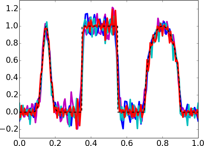
(a) standard CG method (4)

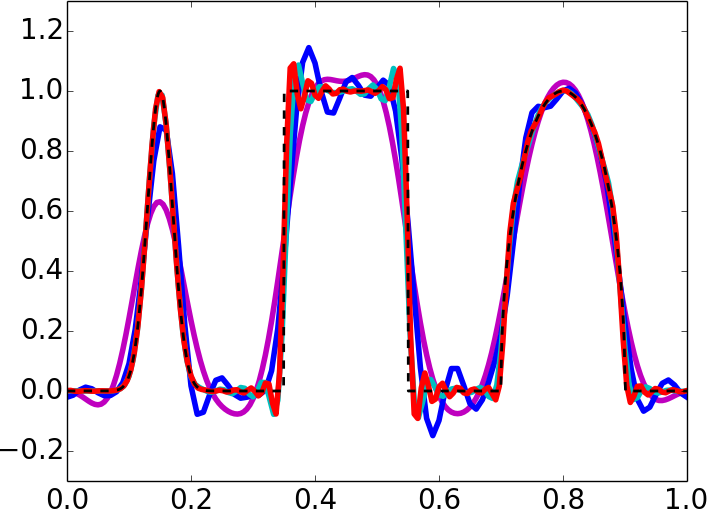
(b) HO-VMS with $\omega=0.1$

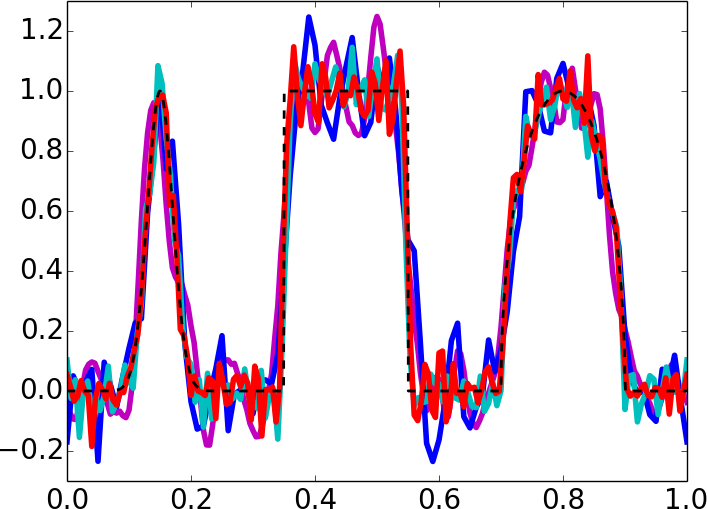
(c) HO-VMS-EV with $\omega=0$

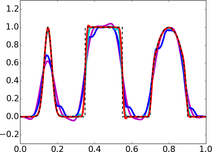
(d) HO-VMS-EV with $\omega=0.1$

Figure 1: One-dimensional linear advection problem (52) with initial condition (63). Numerical solutions at $t=100$ obtained with stabilized high-order methods using $N_{h}=200$ DoFs.

7.2 One-dimensional inviscid Burgers equation

To study the shock-capturing capabilities of entropy stabilization in the context of nonlinear problems, we apply our HO-X-EV methods to the inviscid Burgers equation

$$\frac{\partial u}{\partial t}+\frac{\partial(u^{2}/2)}{\partial x}=0\quad\mbox{in}\quad\Omega=(0,1).$$ (64)

The smooth initial condition is given by

$$u_{0}(x)=\sin(2\pi x).$$ (65)

The entropy solution of this initial value problem develops a shock at the critical time $t_{c}=\frac{1}{2\pi}$. For $t<t_{c}$, the smooth exact solution is defined by the nonlinear equation

$$u(x,t)=\sin(2\pi(x-u(x,t)t))$$ (66)

which can be derived using the method of characteristics.

We evolve the HO-X and HO-X-EV approximations up to the final time $t=0.1$ and measure the EOCs w.r.t. the $L^{1}$ norm. The discretization in time is again performed using the 6th order Runge-Kutta method with the Butcher tableau (62). The results of our grid convergence studies are presented in Table 2. All methods under investigation deliver the optimal rates of convergence.

	HO-SUPG-EV		HO-VMS-EV
$N_{h}$	$\|u_{h}-u_{\text{exact}}\|_{L^{1}}$	EOC	$\|u_{h}-u_{\text{exact}}\|_{L^{1}}$	EOC
8	5.06E-02	–	5.42E-02	–
16	9.27E-03	2.45	1.03E-02	2.39
32	1.75E-03	2.41	2.05E-03	2.33
64	3.90E-04	2.16	4.03E-04	2.35
128	9.17E-05	2.09	9.35E-05	2.11
256	2.25E-05	2.03	2.28E-05	2.04

(a) $p=1$

	HO-SUPG-EV		HO-VMS-EV
$N_{h}$	$\|u_{h}-u_{\text{exact}}\|_{L^{1}}$	EOC	$\|u_{h}-u_{\text{exact}}\|_{L^{1}}$	EOC
16	5.48E-03	–	5.41E-03	–
32	5.57E-04	3.30	6.15E-04	3.14
64	1.31E-04	2.08	1.53E-04	2.01
128	1.78E-05	2.88	1.91E-05	3.01
256	2.29E-06	2.96	2.32E-06	3.04
512	2.86E-07	3.00	2.87E-07	3.02

(b) $p=2$

	HO-SUPG-EV		HO-VMS-EV
$N_{h}$	$\|u_{h}-u_{\text{exact}}\|_{L^{1}}$	EOC	$\|u_{h}-u_{\text{exact}}\|_{L^{1}}$	EOC
24	7.30E-04	–	7.42E-04	–
48	2.16E-04	1.76	2.34E-04	1.66
96	1.43E-05	3.91	1.86E-05	3.66
192	7.96E-07	4.17	1.30E-06	3.83
384	4.94E-08	4.01	8.70E-08	3.91
768	3.12E-09	3.99	5.61E-09	3.96

(c) $p=3$

	HO-SUPG-EV		HO-VMS-EV
$N_{h}$	$\|u_{h}-u_{\text{exact}}\|_{L^{1}}$	EOC	$\|u_{h}-u_{\text{exact}}\|_{L^{1}}$	EOC
32	6.03E-04	–	6.26E-04	–
64	3.72E-05	4.02	4.14E-05	3.92
128	4.66E-07	6.32	7.11E-07	5.86
256	3.54E-08	3.72	4.47E-08	3.99
512	1.07E-09	5.05	1.16E-09	5.26
1024	3.28E-11	5.03	3.45E-11	5.07

(d) $p=4$

Table 2: One-dimensional inviscid Burgers equation (64) with initial condition (65). Grid convergence history for stabilized high-order methods using finite elements of degree $p\in\{1,2,3,4\}$.

Let us now run the simulations up to $t=10$ and study the ability of the stabilized HO methods to capture the shock that forms at $t=t_{c}$. Computations are performed using piecewise-polynomial finite element spaces of degree $p=\{1,2,4,8\}$. In all numerical experiments, we use $N_{h}=128$ DoFs. The results obtained with HO-X and HO-X-EV are shown in Figs 2a–2d. We remark that our simulations became unstable for HO-SUPG with $p=\{4,8\}$ and HO-VMS with $p=8$. The use of entropy stabilization has cured this problem. In addition, it reduced the magnitude of spurious oscillations in all cases. The nonoscillatory solutions shown in Figs 2e–2h were obtained using the monolithic convex limiting techniques of Section 5. It can be seen that the flux-limited (FL) version of each high-order method enforces local bounds without introducing large amounts of numerical diffusion. The differences between the FL solutions are marginal, which indicates that the choice of high-order stabilization for the limiting target is of minor importance for this particular test problem.

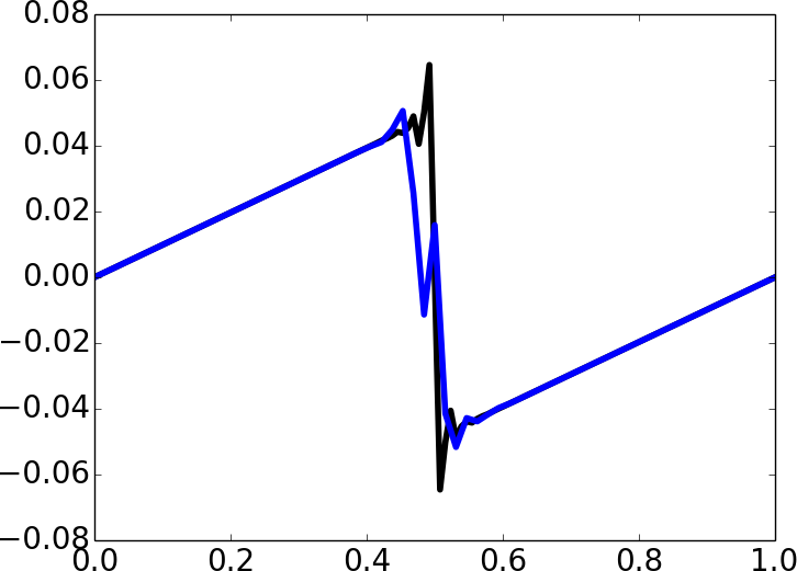
(a) HO-SUPG

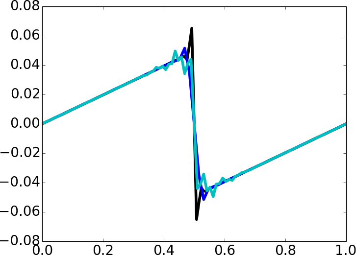
(b) HO-VMS

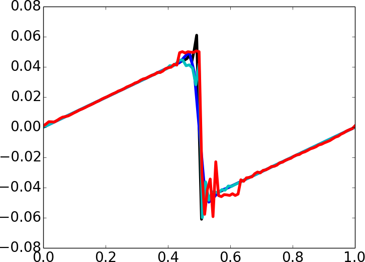
(c) HO-SUPG-EV

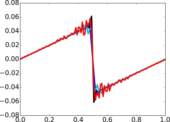
(d) HO-VMS-EV

(e) HO-SUPG-FL

(f) HO-VMS-FL

(g) HO-SUPG-EV-FL

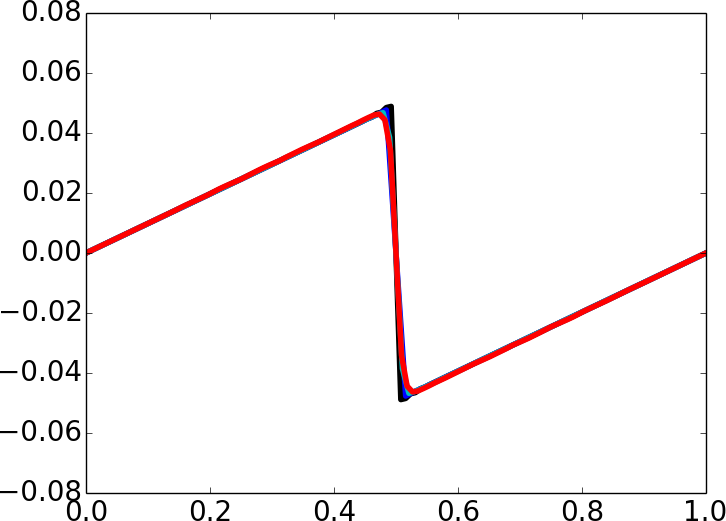
(h) HO-VMS-EV-FL

Figure 2: One-dimensional Burgers equation (64) with initial condition (65). Numerical solutions at $t=10$ obtained using $N_{h}=128$ DoFs.

7.3 Two-dimensional solid body rotation

To facilitate a comparison with the $\mathbb{P}_{1}/\mathbb{Q}_{1}$ version of algebraic flux correction schemes and variational approaches to shock capturing, let us consider the solid body rotation benchmark [25, 24, 29]. In this two-dimensional experiment, we solve the unsteady linear advection equation

$$\frac{\partial u}{\partial t}+\nabla\cdot(\mathbf{v}u)=0\quad\mbox{in}\quad\Omega=(0,1)^{2}$$ (67)

using the divergence-free velocity field ${\bf v}(x,y)=2\pi(0.5-y,x-0.5)$ and the initial condition [29]

$$u_{0}(x,y)=\begin{cases}u_{0}^{\rm hump}(x,y)&\text{if}\ \sqrt{(x-0.25)^{2}+(y-0.5)^{2}}\leq 0.15,\\ u_{0}^{\rm cone}(x,y)&\text{if}\ \sqrt{(x-0.5)^{2}+(y-0.25)^{2}}\leq 0.15,\\ 1&\text{if}\ \begin{cases}\left(\sqrt{(x-0.5)^{2}+(y-0.75)^{2}}\leq 0.15\right),\\ \left(|x-0.5|\geq 0.025,~{}y\geq 0.85\right),\end{cases}\\ 0&\text{otherwise},\end{cases}$$ (68a)

where

$$u_{0}^{\rm hump}(x,y) =\frac{1}{4}+\frac{1}{4}\cos\left(\frac{\pi\sqrt{(x-0.25)^{2}+(y-0.5)^{2}}}{0.15}\right),$$ (68b)

$$u_{0}^{\rm cone}(x,y) =1-\frac{\sqrt{(x-0.5)^{2}+(y-0.25)^{2}}}{0.15}.$$ (68c)

The so-defined initial data undergoes counterclockwise rotation around the center $(0.5,0.5)$ of the domain $\Omega$. After each complete revolution (i.e., for $t\in\mathbb{N}$), the exact solution coincides with $u_{0}$.

Numerical solutions are evolved up to $t=1$ using finite elements of degree $p=\{1,2,4\}$. For all values of $p$, we choose the mesh size corresponding to $N_{h}=128^{2}$ DoFs. The results obtained with the entropy stable HO-VMS-EV method are shown in Fig. 3a-3c. It can be seen that the discontinuity-capturing effect of EV stabilization is not enough to secure the IDP property w.r.t. $\mathcal{G}=[0,1]$. The flux-limited scheme HO-VMS-EV-BP yields the bound-preserving solutions shown in Figs 3d-3f. The discontinuities are resolved in a nonoscillatory manner but the imposition of local maximum principles results in unnecessary limiting at smooth local extrema. To avoid the loss of high-order accuracy around smooth traveling peaks, the local bounds of the subcell flux limiting procedure can be relaxed using smoothness indicators, for a presentation of which we refer the reader to [17, 27, 30]. The results presented in Figs 3g-3i were obtained with the entropy-aware HO-VMS-EV-FL version of the flux-limited scheme (33). In accordance with Remark 6, the unnecessary imposition of the entropy stability condition (41) increases the levels of numerical dissipation and the magnitude of the $L^{1}$ error. We conclude that limiting based on the local BP property is sufficient for linear advection problems.

$||u_{h}-u_{\text{exact}}||_{L^{1}}=2.67\times 10^{-2}$

$u_{h}\in[-4.6\times 10^{-3},~{}1.002]$

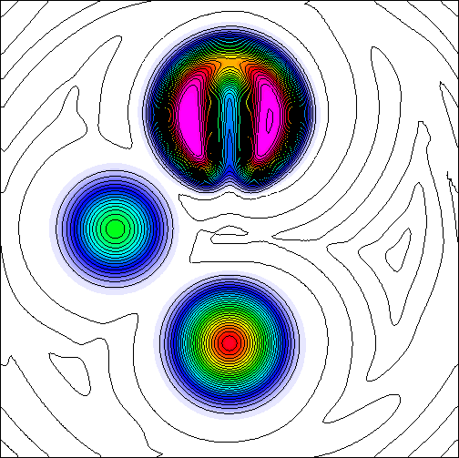
(a) HO-VMS-EV, $p=1$

$||u_{h}-u_{\text{exact}}||_{L^{1}}=1.63\times 10^{-2}$

$u_{h}\in[-8\times 10^{-4},~{}0.9929]$

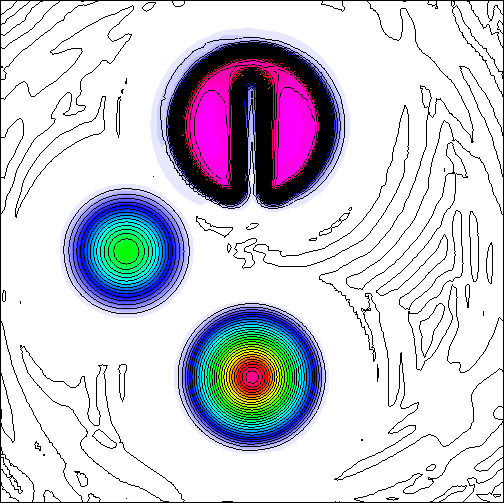
(b) HO-VMS-EV, $p=2$

$||u_{h}-u_{\text{exact}}||_{L^{1}}=9.96\times 10^{-3}$

$u_{h}\in[-3.1\times 10^{-2},~{}1.044]$

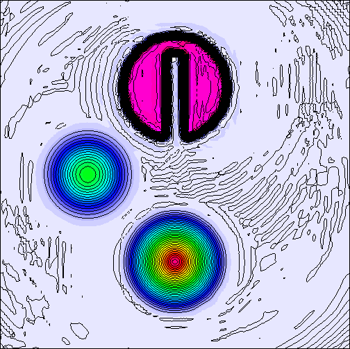
(c) HO-VMS-EV, $p=4$

$||u_{h}-u_{\text{exact}}||_{L^{1}}=2.80\times 10^{-2}$

$u_{h}\in[2.02\times 10^{-24},~{}0.9814]$

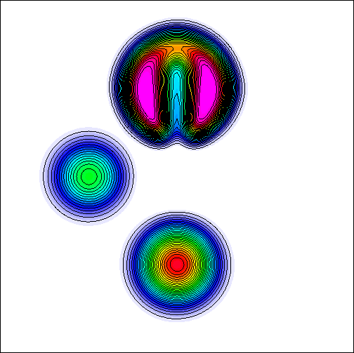
(d) HO-VMS-EV-BP, $p=1$

$||u_{h}-u_{\text{exact}}||_{L^{1}}=2.49\times 10^{-2}$

$u_{h}\in[6.06\times 10^{-23},~{}0.9865]$

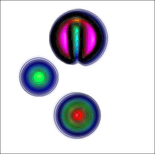
(e) HO-VMS-EV-BP, $p=2$

$||u_{h}-u_{\text{exact}}||_{L^{1}}=2.11\times 10^{-2}$

$u_{h}\in[2.59\times 10^{-19},~{}0.9862]$

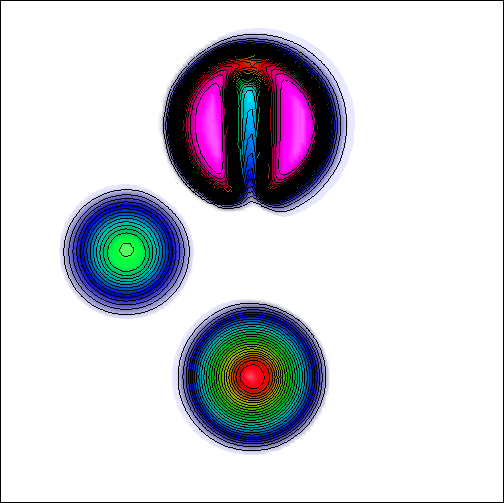
(f) HO-VMS-EV-BP, $p=4$

$||u_{h}-u_{\text{exact}}||_{L^{1}}=3.67\times 10^{-2}$

$u_{h}\in[2.16\times 10^{-11},~{}0.9195]$

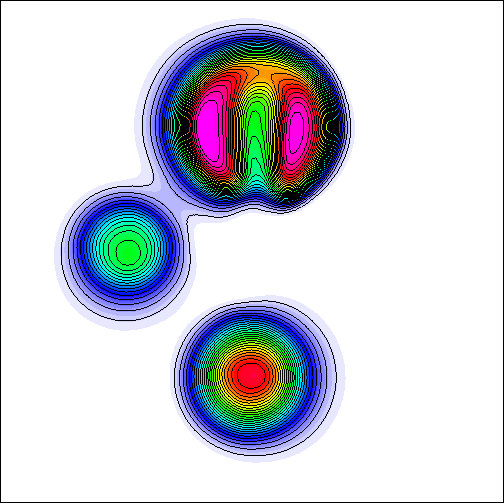
(g) HO-VMS-EV-FL, $p=1$

$||u_{h}-u_{\text{exact}}||_{L^{1}}=4.37\times 10^{-2}$

$u_{h}\in[9.3\times 10^{-8},~{}0.8778]$

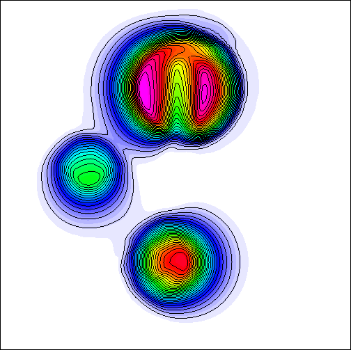
(h) HO-VMS-EV-FL, $p=2$

$||u_{h}-u_{\text{exact}}||_{L^{1}}=5.22\times 10^{-2}$

$u_{h}\in[4.37\times 10^{-6},~{}0.7901]$

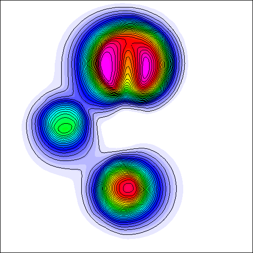
(i) HO-VMS-EV-FL, $p=4$

Figure 3: Solid body rotation problem (67) with initial condition (68). Numerical solutions at $t=1$ obtained using $N_{h}=128^{2}$ DoFs. In each diagram, we plot 30 contour lines corresponding to a uniform subdivision of $\mathcal{G}=[0,1]$.

7.4 Buckley-Leverett equation

The first two-dimensional nonlinear problem that we consider is the Buckley-Leverett equation [9, 28]. The nonconvex flux function of the nonlinear conservation law to be solved is

$$\mathbf{f}(u)=\frac{u^{2}}{u^{2}+(1-u)^{2}}(1,1-5(1-u)^{2}).$$ (69)

The computational domain is $\Omega_{h}=(-1.5,1.5)^{2}$. The piecewise-constant initial condition is given by

$$u_{0}(x,y)=\begin{cases}1&\mbox{ if }x^{2}+y^{2}<0.5,\\ 0&\mbox{ otherwise}.\end{cases}$$ (70)

The exact solution of this nonlinear problem exhibits a rotating wave structure. For entropy stabilization purposes, we use $\eta(u)=\frac{u^{2}}{2}$. The corresponding entropy flux is $\mathbf{q}(u)=(q_{x}(u),q_{y}(u))$, where

$$q_{x} =\frac{1}{4}\left[\frac{2(u-1)}{2u^{2}-2u+1}-\log(2u^{2}-2u+1)\right],$$ (71)

$$q_{y} =\frac{1}{12}\left[-20u^{3}+15u^{2}-\frac{9u+6}{2u^{2}-2u+1}-3\log(2u^{2}-2u+1)-15\tan^{-1}(1-2u)\right].$$ (72)

An upper bound for the fastest wave speed can be found in [9]. We overestimate it by using $\lambda=3.4$.

Simulations are performed using $N_{h}=128^{2}$ DoFs for $p\in\{1,2,4\}$. The HO-VMS-EV-FL results at $t=0.5$ are shown in Fig. 4. They exhibit a crisp resolution of curved shocks and are invariant domain preserving w.r.t. $\mathcal{G}\in[0,1]$. The maximal values listed above the plots decrease slightly as the polynomial degree $p$ is increased while keeping $N_{h}$ fixed. However, the subcell flux limiting strategy makes it possible to avoid a far more dramatic increase in the levels of numerical dissipation due to extended stencils of high-order finite element approximations (as reported, e.g., in [30]).

$u_{h}\in[0,~{}0.9993]$

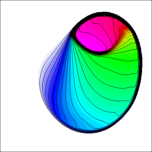
(a) $p=1$

$u_{h}\in[0,~{}0.993]$

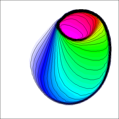
(b) $p=2$

$u_{h}\in[0,~{}0.9893]$

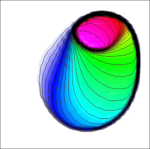
(c) $p=4$

Figure 4: Buckley-Leverett equation (69) with initial condition (70). Numerical solutions at $t=0.5$ obtained with HO-VMS-EV-FL using $N_{h}=128^{2}$ DoFs and Bernstein finite elements of degree $p=\{1,2,4\}$. In each diagram, we plot 30 contour lines corresponding to a uniform subdivision of $\mathcal{G}=[0,1]$.

7.5 KPP problem

In the last numerical example, we consider the KPP problem [15, 16, 23], a challenging nonlinear test for verification of entropy stability properties. Equation (1a) with the nonconvex flux function

$$\mathbf{f}(u)=(\sin(u),\cos(u))$$ (73)

is solved in the computational domain $\Omega_{h}=(-2,2)\times(-2.5,1.5)$ using the initial condition

$$u_{0}(x,y)=\begin{cases}\frac{7\pi}{2}&\mbox{if}\quad\sqrt{x^{2}+y^{2}}\leq 1,\\ \frac{\pi}{4}&\mbox{otherwise}.\end{cases}$$ (74)

The entropy flux corresponding to $\eta(u)=\frac{u^{2}}{2}$ is $\mathbf{q}(u)=(u\sin(u)+\cos(u),u\cos(u)-\sin(u))$. A simple upper bound for the maximal speed is $\lambda=1$. More accurate estimates can be found in [16].

Similarly to the Buckley-Leverett problem, the entropy solution of the KPP problem exhibits a two-dimensional rotating wave structure. The main challenge of this test is to prevent possible convergence to wrong weak solutions. Even bound-preserving high-resolution schemes may fail to preserve the thin gap between the twisted shocks if no entropy viscosity is added [16, 28]. The results displayed in Fig. 5 were obtained with HO-VMS-EV-FL using $N_{h}=128^{2}$ DoFs for Bernstein finite elements of degree $p=\{1,2,4\}$. The snapshots correspond to the final time $t=1$ and reproduce the rotating wave structure of the entropy solution correctly (cf. [16, 26, 28]). The two shocks remain clearly separated and the ranges of the numerical solutions stay in the invariant set $\mathcal{G}=[\frac{1}{4}\pi,~{}\frac{7}{2}\pi]$.

$u_{h}\in[0.7854,~{}10.9955]$

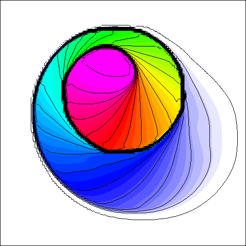
(a) $p=1$

$u_{h}\in[0.7854,~{}10.9955]$

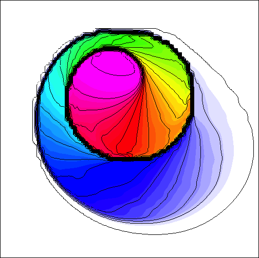
(b) $p=2$

$u_{h}\in[0.7854,~{}10.9955]$

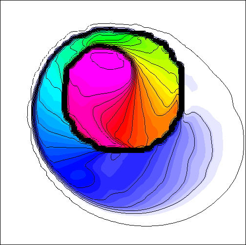
(c) $p=4$

Figure 5: KPP problem [23] with initial condition (74). Numerical solutions at $t=1$ obtained with HO-VMS-EV-FL using $N_{h}=128^{2}$ DoFs and Bernstein finite elements of degree $p=\{1,2,4\}$. In each diagram, we plot 30 contour lines corresponding to a uniform subdivision of $\mathcal{G}=[\frac{1}{4}\pi,~{}\frac{7}{2}\pi]$.

8 Conclusions

The presented research was aimed at exploring the aspects of entropy stability in the context of high-order continuous finite element approximations to hyperbolic conservation laws. We proved that the continuous Galerkin method is square entropy conservative, endowed it with high-order stabilization terms, and designed property-preserving limiters for high-order Bernstein finite elements. It is hoped that the proposed methodology paves the way for further analysis and design of nonlinear high-resolution finite element schemes equipped with entropy correction procedures. In particular, we envisage that extensions of the new entropy fixes to hyperbolic systems and discontinuous Galerkin methods should be relatively straightforward. More challenging open problems include theoretical investigations of the steady-state limit, development of efficient iterative solvers for nonlinear discrete problems, and provable preservation of entropy stability in fully discrete flux-corrected schemes.

Acknowledgments

The work of Dmitri Kuzmin was supported by the German Research Association (DFG) under grant KU 1530/23-1. The authors would like to thank Hennes Hajduk (TU Dortmund University) for suggesting an improved version of the subcell flux decomposition.

References

- [1] R. Abgrall, A general framework to construct schemes satisfying additional conservation relations. Application to entropy conservative and entropy dissipative schemes. J. Comput. Phys. 372 (2018) 640–666.
- [2] R. Abgrall, P. Öffner, and H. Ranocha, Reinterpretation and extension of entropy correction terms for residual distribution and discontinuous Galerkin schemes. Preprint arXiv: 1908.04556v1, 2019.
- [3] R. Anderson, A. Barker, J. Bramwell, J.-S. Camier, J. Cerveny, V. Dobrev, Y. Dudouit, A. Fisher, Tz. Kolev, W. Pazner, M. Stowell, V. Tomov, J. Dahm, D. Medina, and S. Zampini, MFEM: a modular finite element library. arXiv preprint 1911.09220. Web site: https://mfem.org.
- [4] R. Anderson, V. Dobrev, Tz. Kolev, D. Kuzmin, M. Quezada de Luna, R. Rieben, and V. Tomov, High-order local maximum principle preserving (MPP) discontinuous Galerkin finite element method for the transport equation. J. Comput. Phys. 334 (2017) 102–124.
- [5] G. Barrenechea, V. John, and P. Knobloch, Analysis of algebraic flux correction schemes. SIAM J. Numer. Anal. 54 (2016) 2427–2451.
- [6] A.N. Brooks and T.J.R. Hughes, Streamline upwind Petrov-Galerkin formulations for convection dominated flows with particular emphasis on the incompressible Navier-Stokes equations. Comput. Methods Appl. Mech. Engrg. 32 (1982) 199–259.
- [7] E. Burman, Consistent SUPG-method for transient transport problems: Stability and convergence. Comput. Methods Appl. Mech. Engrg. 199 (2010) 1114–1123.
- [8] T. Chen and C.W. Shu, Entropy stable high order discontinuous Galerkin methods with suitable quadrature rules for hyperbolic conservation laws. J. Comput. Phys. 345 (2017) 427–461.
- [9] I. Christov and B. Popov, New non-oscillatory central schemes on unstructured triangulations for hyperbolic systems of conservation laws. J. Comput. Phys. 227-11, (2008) 5736–5757.
- [10] S. Gottlieb, C.-W. Shu, and E. Tadmor, Strong stability-preserving high-order time discretization methods. SIAM Review 43 (2001) 89–112.
- [11] J. C. Butcher, On Runge-Kutta processes of high order. J. of the Australian Mathematical Society 4-2, (1964) 179–194.
- [12] J.-L. Guermond and M. Nazarov, A maximum-principle preserving finite element method for scalar conservation equations. Computer Methods Appl. Mech. Engrg. 272 (2014) 198–213.
- [13] J.-L. Guermond, M. Nazarov, B. Popov, and I. Tomas, Second-order invariant domain preserving approximation of the Euler equations using convex limiting. SIAM J. Sci. Computing 40 (2018) A3211-A3239.
- [14] J.-L. Guermond, R. Pasquetti, and B. Popov, Entropy viscosity method for nonlinear conservation laws. J. Comput. Phys. 230 (2011) 4248–4267.
- [15] J.-L. Guermond and B. Popov, Invariant domains and first-order continuous finite element approximation for hyperbolic systems. SIAM J. Numer. Anal. 54 (2016) 2466–2489.
- [16] J.-L. Guermond and B. Popov, Invariant domains and second-order continuous finite element approximation for scalar conservation equations. SIAM J. Numer. Anal. 55 (2017) 3120–3146.
- [17] H. Hajduk, D. Kuzmin, Tz. Kolev, V. Tomov, I. Tomas and J.N. Shadid, Matrix-free subcell residual distribution for Bernstein finite elements: Monolithic limiting. Computers & Fluids. 200 (2020) 104–451
- [18] H. Hajduk, Monolithic convex limiting in discontinuous Galerkin discretizations of hyperbolic conservation laws. In preparation.
- [19] G. S. Jiang and C.-W. Shu, On a cell entropy inequality for discontinuous Galerkin methods. Mathematics of Computation 62 (1994) 531–538.
- [20] V. John and J. Novo, Error analysis of the SUPG finite element discretization of evolutionary convection-diffusion-reaction equations. SIAM J. Numer. Anal. 49 (2011) 1149–1176.
- [21] V. John, S. Kaya, and W. Layton, A two-level variational multiscale method for convection-dominated convection–diffusion equations. Comput. Methods Appl. Mech. Engrg. 195 (2006) 4594–4603.
- [22] S. Kivva, Entropy stable flux correction for scalar hyperbolic conservation laws. Preprint arXiv:2004.02258 [math.NA], 2020.
- [23] A. Kurganov, G. Petrova, and B. Popov, Adaptive semidiscrete central-upwind schemes for nonconvex hyperbolic conservation laws. SIAM J. Sci. Comput. 29 (2007) 2381–2401.
- [24] D. Kuzmin, Algebraic flux correction I. Scalar conservation laws. In: D. Kuzmin, R. Löhner and S. Turek (eds.) Flux-Corrected Transport: Principles, Algorithms, and Applications. Springer, 2nd edition: 145–192 (2012).
- [25] D. Kuzmin, Monolithic convex limiting for continuous finite element discretizations of hyperbolic conservation laws. Comput. Methods Appl. Mech. Engrg. 361 (2020) 112804.
- [26] D. Kuzmin, Entropy stabilization and property-preserving limiters for discontinuous Galerkin discretizations of nonlinear hyperbolic equations. Preprint arXiv:2004.03521 [math.NA], 2020.
- [27] D. Kuzmin and M. Quezada de Luna, Subcell flux limiting for high-order Bernstein finite element discretizations of hyperbolic conservation laws. J. Comput. Phys. Available online 21 March 2020, 109411, https://doi.org/10.1016/j.jcp.2020.109411
- [28] D. Kuzmin and M. Quezada de Luna, Algebraic entropy fixes and convex limiting for continuous finite element discretizations of scalar hyperbolic conservation laws. Preprint arXiv:2003.12007 [math.NA], 2020.
- [29] R.J. LeVeque, High-resolution conservative algorithms for advection in incompressible flow. SIAM Journal on Numerical Analysis 33, (1996) 627–665.
- [30] C. Lohmann, D. Kuzmin, J.N. Shadid, and S. Mabuza, Flux-corrected transport algorithms for continuous Galerkin methods based on high order Bernstein finite elements. J. Comput. Phys. 344 (2017) 151-186.
- [31] A. Quarteroni and A. Valli, Numerical Approximation of Partial Differential Equations. Springer, 1994.
- [32] E. Tadmor, The numerical viscosity of entropy stable schemes for systems of conservation laws I. Math. Comp. 49 (1987) 91–103.
- [33] E. Tadmor, Entropy stability theory for difference approximations of nonlinear conservation laws and related time-dependent problems. Acta Numerica (2003) 451–512.