Cross-correlating 2MRS galaxies with UHECR flux from Pierre Auger Observatory

Abstract

We apply a recently proposed cross-correlation power spectrum technique to study relationship between the ultra-high energy cosmic ray (UHERC) flux from the Pierre Auger Observatory and galaxies from the 2MASS Redshift Survey. Using a simple linear bias model relative to the galaxy auto power spectrum, we are able to constrain the value of bias to be less than 1% for UHECR with energies 4 EeV - 8 EeV, less than 2.3% for UHECR with energies above 8 EeV and less than 21% for UHECR with energies above 52 EeV (all 95% confidence limit). We study energy dependence of the bias, but the small sample size does not allow us to reach any statistically significant conclusions. For the cosmic ray events above 52 EeV we discover a curious excess cross-correlation at $\sim 1^{\circ}$ degree scales. Given similar cross-correlation is not visible at larger angular scales, statistical fluctuation seems like the most plausible explanation.

I Introduction

The quest to find the astrophysical sources of ultra-high energy cosmic rays (UHECR) and to understand the physical mechanisms that accelerate particles to energies over 1 EeV is still underway (see Alves Batista et al. (2019) for a recent review). Although recently the Pierre Auger (PA) collaboration achieved a major breakthrough in discovering a dipolar modulation of the UHECR flux above 8 EeV Aab et al. (2017), this does not provide sufficient information to resolve these puzzles. Smaller scale UHECR anisotropies would provide further clues, but they so far escape a conclusive detection, despite several suggestive hints Abbasi et al. (2014); Aab et al. (2018).

There exists extensive literature dealing with the issue of UHECR anisotropies (see e.g. Kashti and Waxman (2008); Koers and Tinyakov (2009); di Matteo et al. (2018, 2020); Aab et al. (2018); Abbasi et al. (2018a); Tinyakov (2018); Oikonomou et al. (2013); Aab et al. (2015a); Abbasi et al. (2018b, 2014); Denton and Weiler (2015) and references therein). One strategy is to focus exclusively on the UHECR data. Using them, it is possible to search for “hotspots” Abbasi et al. (2014); Aab et al. (2015a), constrain individual coefficients in the spherical harmonic expansion and the related angular power spectra of map of the UHECR flux di Matteo et al. (2018); Denton and Weiler (2015) or investigate the correlation function Tinyakov (2018); Aab et al. (2015a). Alternatively, one can search for a connection between the observed directions of the UHECR events and the distribution of objects in the nearby Universe. Beyond again looking at the correlation function di Matteo et al. (2020); Aab et al. (2015a), it is also possible Kashti and Waxman (2008); Koers and Tinyakov (2009); Oikonomou et al. (2013); Tinyakov (2018); di Matteo et al. (2018); Aab et al. (2018, 2015a); Ahlers et al. (2018) to build an expected UHECR flux based on a particular physical model for the sources and the magnetic fields and compare the observed distribution of UHECR with the expectation of the model, for example using the Kolmogorov-Smirnov statistic or by comparing likelihood ratios of various models.

Recently, Urban et al. (2020) proposed using harmonic space cross-correlation power spectrum (see Eq. 3) of the UHECR flux and a tracer of the large scale structure as a novel addition to the later family of approaches. Effectively, it compresses the two dimensional information contained in the two maps into a one dimensional cross power spectrum $C_{\ell}^{XY}$ that quantifies coherence of features in the maps as a function of the angular scale. Such compression would be detrimental for example in case the UHECR are produced by several nearby sources and information on the map level would be expected to be essential. On the other hand, in the case of a large number of sources tracing the large scale structure, information about any particular sky direction is not important and it is mostly the overall coherence between UHECR and the tracer that carries the relevant information. In such case reducing the dimensionality of the data can be advantageous. Even if we find that the UHECR flux is dominated by several nearby sources, analysis based on the cross-correlation power spectra might be useful to understand the properties of the residual flux after these sources are modeled and subtracted out.

The usefulness of the cross-power spectrum analysis also depends on the effect the magnetic fields have on the UHECR propagation. If the magnetic fields cause mostly a stochastic deflection of UHECR, this should manifest effectively as smearing of the signal below a certain smoothing scale. The cross-power spectrum technique would then still be useable on angular scales larger than such smoothing scale, with the value of the smoothing scale providing information about the properties of the magnetic field. On the other hand, if the effects of the magnetic field turn out to be more complicated, map based analysis may again turn out to be necessary.

Notice that the cross-correlation technique does not depend on any particular physical model (of for example the magnetic field) beyond choosing the particular tracer to cross-correlate with. This means that it is well suited for initial explorations, findings of which can inform more complex physical models.

While the proposed technique is at heart related to the other commonly used techniques (for example the cross-power spectrum is a Fourier transform of the real space correlation function), it offers certain advantages. In particular, it offers a clean separation of angular scales, which may offer additional insights. In commonly used methods similar information could be obtainable by comparing results obtained with different smoothing scales, but this can quickly become rather involved.

In this work we perform the first application of the cross-correlation power spectrum technique to a UHECR data set, namely events detected by the PA Observatory (PAO). We cross-correlate the corresponding UHECR flux with galaxies from the 2MASS Redshift Survey (2MRS); by doing this we effectively probe how much do the UHECR events trace all the visible matter in the nearby Universe. As a possible alternative one can perform a targeted analysis by picking a particular set of objects deemed likely to contribute to the UHECR flux (such as starburst galaxies) and cross correlate the UHECR flux with them, but we do not perform such a targeted analysis in this work.

The ultimate question we will aim to answer is whether there is any excess correlation between the 2MRS and PAO datasets. While the cross-correlation does not need to assume any particular model (see the points in Fig. 1), we fit a simple linear bias model relative to the 2MRS galaxy auto power spectrum to gauge to what extent are the data consistent with no correlation. To the extent allowed by the publicly available data we will also investigate dependence of the bias on the energies of the UHECR events.

This work is organized as follows: We start by summarizing the data sets we use in § II. In § III we describe the steps used in our analysis, before presenting our results in § IV. We list tests we performed to check robustness of our results in § V and conclude with a discussion in § VI. In the Appendix A we describe how we calculate the exposure of the Pierre Auger Observatory.

II Data

We use the PAO data publicly released with Aab et al. (2017), representing over 12 years of observing. We mostly focus on the 32187 UHECR events with energies above 8 EeV, although we briefly discuss also the 81701 events with energies between 4 and 8 EeV. Beyond this binary division we do not have any further information about the energies of the events, with the exception of a subset of 231 events with energies above 52 EeV which were released earlier and which correspond to about 10 years of data collecting Aab et al. (2015a). For a technical description of the PAO and the detection techniques, we refer the reader to Aab et al. (2015b).

As a tracer of the nearby large scale structure we use galaxies from the 2MRS Huchra et al. (2012). This spectroscopic survey covers 91% of sky and contains 43533 galaxies, forming a nearly complete (97.6%) survey of galaxies brighter than 11.75 mag in $K_{s}$ band, with reddening limited to $E(B-V)\leq 1\,\mathrm{mag}$.

III Analysis techniques

In this section we go over the technical details of our analysis. We first describe how we convert the catalogs of UHECR events and galaxies into sky maps, how we estimate their cross power spectra and introduce our linear bias model. Then we go on and detail the generation of mock UHECR catalogs, comment on obtaining auto power spectra of the 2MRS galaxy catalog and finish by explaining a maximum likelihood estimate for the bias parameter of our model.

III.1 Maps and masks

We work with maps in the Healpix pixelization Gorski et al. (2005). Our default resolution will be $N_{\mathrm{side}}=512$, with each pixel having an area of 47 square arc minutes.

From the 2MRS data, we construct the galaxy overdensity map

$$\delta^{g}(\vec{n})=\frac{n_{g}(\vec{n})-\bar{n}_{g}}{\bar{n}_{g}},$$ (1)

where $n_{g}$ denotes the number of galaxies in a given pixel and $\bar{n}_{g}$ is the mean value over all observed pixels. Only galaxies with galactic latitude $b$ and longitude $l$ satisfying

$$|b|\geq\begin{cases}5^{\circ},\ \ \ 30^{\circ}\leq l\leq 330^{\circ}\\ 8^{\circ},\ \ \ \text{otherwise}\\ \end{cases}$$ (2)

were included into the catalog; this determines the mask of the survey which we will use in what follows.

From the UHECR catalog we first convert the observed hit counts into a flux map $\Phi$ by using an estimated exposure function (25) from Appendix A. Then we calculate the overdensity map $\delta^{\Phi}$ in a manner analogous to (1). The mask is determined by the maximal declination that can be observed by PAO.

III.2 Power spectra and linear bias

Given two fields on a sphere $\delta^{X},\delta^{Y}$, their cross power spectrum is calculated as

$$\hat{C}^{XY}_{\ell}=\sum_{m}\frac{\delta^{X}_{\ell m}\delta^{Y*}_{\ell m}}{2\ell+1},$$ (3)

where $\delta^{X,Y}_{\ell m}$ are coefficients of $\delta^{X,Y}$ in the spherical harmonic expansion and star denotes complex conjugation. For brevity, in what follows we will not explicitly write the hat on top of power spectra to denote an estimate.

The model we will consider in this work is a linear relationship between the cross-power spectra of $\delta^{\Phi}$ and $\delta^{g}$, the UHECR flux and galaxy counts overdensities, and the galaxy overdensity auto power spectrum,

$$C^{\Phi g}_{\ell}=bC^{gg}_{\ell}+N_{\ell}.$$ (4)

Here $N_{\ell}$ represents noise and $b$ is commonly referred to as “bias”. In this work we will estimate value of $b$ to see whether it is consistent with zero, which would mean no relationship between the anisotropies in the observed UHECR flux and the 2MRS galaxies.

Because of the incomplete sky coverage, we do not know $\delta^{X}$ over the whole sky. Effectively we can think of this as measuring $\delta^{X}$ modulated with a position-dependent weight $w^{X}$, i.e.

$$\tilde{\delta}^{g}(\vec{n})=w^{g}(\vec{n})\delta^{g}(\vec{n}).$$ (5)

In the simplest case, $w^{X}$ represents a binary mask and is set to zero in parts of the sky not accessible to the experiment and to one elsewhere. In more complicated cases, $w^{X}$ can be used to down-weight the data in parts of the sky where the measurements are relatively noisier. The unobserved pixels are the limiting case, as they can be thought of as being infinitely noisy.

We can then calculate the cross-power spectra of $\tilde{\delta}^{g},\tilde{\delta}^{\Phi}$, so-called pseudo-power spectra $\tilde{C}^{g\Phi}_{\ell}$. Assuming no mixing between different angular scales, these are related to the underlying power spectra through a linear relation (e.g. Hivon et al. (2002))

$$\tilde{C}^{g\Phi}_{\ell}=\sum_{\ell^{\prime}}K_{\ell\ell^{\prime}}C^{g\Phi}_{\ell^{\prime}},$$ (6)

where the kernel $K_{\ell\ell^{\prime}}$ can be analytically calculated from the weights $w^{X}$. For our weights the kernels will be invertible, which allows us to express

$$C^{g\Phi}_{\ell}=\sum_{\ell^{\prime}}K_{\ell\ell^{\prime}}^{-1}\tilde{C}^{g\Phi}_{\ell^{\prime}}.$$ (7)

To calculate the pseudo-power spectra and the kernel $K_{\ell\ell^{\prime}}$ we use the publicly available code Polspice Chon et al. (2004).

While for the galaxy overdensity map we use $w^{g}$ based on the 2MRS mask, for the PA events we use the product of the corresponding mask and the exposure function $E(\delta)$ described in Appendix A. This way we put lower weight on events in the parts of the sky with low exposure, that are intrinsically more noisy. We point out that given the underlying Poisson statistics, the choice of weighting of the PAO events leading to the optimal signal to noise ratio is unknown to us and does not appear to be immediately obvious, so we use this as a simple heuristic.

III.3 Random UHECR event catalog

Here we describe how we generate mock UHECR catalogs, necessary to estimate properties of $N_{\ell}$ and uncertainties of our analysis. As we will see shortly, the values of $b$ preferred by the data are rather small and we are not able to rule out $b=0$ with sufficient statistical significance. We will thus simulate UHECR events as if they were independent of the galaxy positions.

We start by generating events from an isotropic flux, consistent with the exposure (25). To accommodate for the dipole observed in the UHECR flux Aab et al. (2017), for each event we first calculate

$$p_{\mathrm{th}}=\frac{1+A_{d}\left(\vec{n}\cdot\vec{n}_{\mathrm{PAd}}\right)}{1+A_{d}},$$ (8)

where $\vec{n}$ is the direction of the generated event, $\vec{n}_{\mathrm{PAd}}$ is the direction of the observed UHECR flux dipole (declination $-24^{\circ}$ and right ascension $100^{\circ}$) and $A_{d}=0.065$ is its amplitude. For each such event we then draw a random number $p$ uniformly distributed in $[0,1]$ and retain the generated event only if $p<p_{\mathrm{th}}$; this leads to a dipole flux modulation. We repeat this procedure until we have the same number of events as is in the UHECR catalog, and we use them to construct a mock overdensity map $\delta^{\Phi}$. The whole process is repeated to generate $N_{\mathrm{sims}}=200$ mock UHECR maps.

III.4 2MRS auto power spectra

To estimate the value of bias $b$ we also need to know the auto power spectrum of the 2MRS galaxy overdensities. To achieve this, we repeat the calculation from Ando et al. (2018).

Because the angular power spectrum estimated from $\delta^{g}$ by Polspice is a sum of the signal and shot noise, we must subtract the latter. To estimate it, we randomly split the 2MRS galaxy catalog into two parts, obtain the corresponding overdensities $\delta^{g,1},\delta^{g,2}$ and form the half-sum and half-difference maps

$$HS = \frac{\delta^{g,1}+\delta^{g,2}}{2}$$ (9)

$$HD = \frac{\delta^{g,1}-\delta^{g,2}}{2}.$$ (10)

As the latter contains on average only the shot noise and no signal, we can estimate the 2MRS galaxy power spectrum as

$$C^{gg}_{\ell}=C^{HS}_{\ell}-C^{HD}_{\ell}.$$ (11)

The power spectrum we get this way is in good agreement with values reported in Ando et al. (2018).

III.5 Fitting $b$

The power spectra $C^{g\Phi}$ obtained from the mock UHECR maps reveal that the expectation value of $N_{\ell}$ is, while small, nonzero (mostly because the generated UHECR events have the dipolar modulation). We calculate its mean value $\langle N_{\ell}\rangle$ from simulations, and define

$$\Delta C^{\Phi g}_{\ell} = C^{\Phi g}_{\ell}-\langle N_{\ell}\rangle$$ (12)

$$\Delta N_{\ell} = N_{\ell}-\langle N_{\ell}\rangle.$$ (13)

We will then try to explain the excess correlation between UHECR and galaxies in the model,

$$\Delta C^{\Phi g}_{\ell}=bC^{gg}_{\ell}+\Delta N_{\ell},$$ (14)

now with noise that has a zero expectation value.

To avoid correlations and have a more Gaussian likelihood, we bin the multipoles with $\Delta\ell=21$, starting with $\ell_{\mathrm{min}}=2$. As the resolving power of PAO at the investigated energies is $\sim 1^{\circ}-2^{\circ}$, we consider either five ($\ell_{\mathrm{max}}=106$) or ten ($\ell_{\mathrm{max}}=211$) bins in our analysis, as these are the approximate $\ell$ ranges that correspond to the angular scales observed. We chose these $\ell_{\mathrm{max}}$ before the analysis, to avoid a posterior bias.

On simulations we checked that the binned $\Delta C^{\Phi g}_{\ell}$ are well described by a Gaussian distribution with a diagonal covariance; these conclusions are not expected to be affected if $b$ turns out to be nonzero but small.

These findings allow us to construct a Gaussian likelihood $\mathcal{L}$ for $b$,

$$-2\log\mathcal{L}=\sum_{B}\left(\Delta C^{\Phi g}_{B}-bC^{gg}_{B}\right)^{2}\sigma_{B}^{-2},$$ (15)

where $B$ sums over bins and $\sigma_{B}$ is standard deviation of $\Delta C^{\Phi g}_{B}$ estimated from the simulations.

Taking the derivative of the right hand side of (15) with respect to $b$, setting it equal to zero and solving for $b$ leads to the maximum likelihood estimator

$$b=\frac{\sum_{B}\Delta C^{\Phi g}_{B}C^{gg}_{B}\sigma_{B}^{-2}}{\sum_{B}\left(C^{gg}_{B}\right)^{2}\sigma_{B}^{-2}}.$$ (16)

Its standard deviation can be read off directly from the $b^{2}$ term in (15) and is equal to

$$\sigma_{b}^{-2}=\sum_{B}\left(C^{gg}_{B}\right)^{2}\sigma_{B}^{-2}.$$ (17)

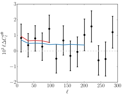
Figure 1: Excess cross-correlation (black points) between the overdensities of the UHECR flux ($E>8\,\mathrm{EeV}$) and galaxy count, together with standard deviations estimated from simulations. The dashed line corresponds to the $b=0$ model, the red and blue line show the best fit linear bias model $bC^{gg}$ with $b$ estimated using data to $\ell_{\mathrm{max}}$ of 106 and 211 respectively.

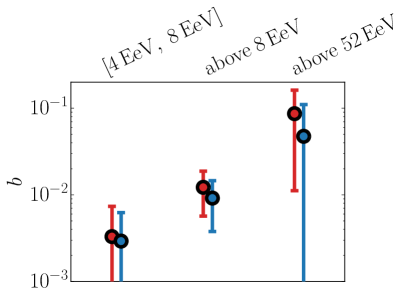
Figure 2: The best fit bias $b$ in three UHECR energy bins. Using the events between 4 EeV and 8 EeV (left), our fiducial sample with energies above 8 EeV (center) and the sample of events with energies above 52 EeV (right, overlaps the fiducial sample). Estimated using data to $\ell_{\mathrm{max}}$ of 106 (red) and 211 (blue).

Table 1: Best fit values of bias

UHECR Energy	$\ell_{\mathrm{max}}$
	$106$	$211$
4 EeV – 8 EeV	$\left(0.33\pm 0.41\right)\times 10^{-2}$	$\left(0.29\pm 0.33\right)\times 10^{-2}$
above 8 EeV	$\left(1.22\pm 0.65\right)\times 10^{-2}$	$\left(0.92\pm 0.54\right)\times 10^{-2}$
above 52 EeV	$\left(8.65\pm 7.54\right)\times 10^{-2}$	$\left(4.74\pm 6.29\right)\times 10^{-2}$

IV Results

In Fig. 1 we show the excess cross-correlation between galaxy and UHECR positions for our fiducial sample of UHECR events with energies over 8 EeV. The case of no bias, $b=0$, is represented by the dashed line, the red and blue curves represent the best fit $bC^{gg}$ when $\ell_{\mathrm{max}}$ is either 106 or 211. The best fit values of $b$ are listed in Table 1, we see a $\sim 1.8\sigma$ detection of positive bias of about a percent. The best fit bias is slightly smaller when the larger range of multipoles $\ell_{\mathrm{max}}$ is used.

We repeat the analysis for the UHECR events with energies between 4 EeV and 8 EeV and for the subset of events we know have energies above 52 EeV and show the resulting values of $b$ in Fig. 2. The best fit values of $b$ are again listed in Table 1.

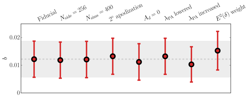
Figure 3: Testing impact of various assumptions (see text) on the outcome of our analysis, with $\ell_{\mathrm{max}}=106$. The left-most point is our fiducial analysis.

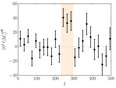
Figure 4: Excess cross-correlation between the overdensities of the flux of UHECR events with energies above 52 EeV and galaxy counts, together with standard deviations estimated from simulations (black points). The orange range shows the region with surprisingly strong cross-correlation.

For the flux of UHECR events with energies above 52 EeV we noticed a strange excess correlation in the multipole range 235 - 295, see Fig. 4. Local significance of the cross correlations observed in these three bins are 3.3$\sigma$, 2.6$\sigma$ and 2.7$\sigma$, which together with their clustering we found interesting enough to report here.

V Tests

For the catalog of events with energies above 8 EeV we repeated the analysis several times with different analysis choices, to test convergence and sensitivity to our assumptions. In Fig. 3 we show the final values of the bias for the case with $\ell_{\mathrm{max}}=106$; $\ell_{\mathrm{max}}=211$ leads to similar conclusions.

We tested:

• halving $N_{\mathrm{side}}$, the resolution of the underlying Healpix grid

• doubling $N_{\mathrm{sim}}$, the number of Monte Carlo simulations

• apodizing the masks with a $2^{\circ}$ cosine taper to ascertain there are no problems with ringing in the Fourier domain

• neglecting the UHECR dipole when generating mock catalogs by setting $A_{d}=0$

• changing $E(\delta)$ by artificially increasing / lowering the PAO latitude $\lambda_{\mathrm{PAO}}$ (see Appendix A) while keeping the observable part of the sky constant through a matching change in $\theta_{\mathrm{max}}$

• weighting the PAO events by $E^{2}(\delta)$ as opposed to $E(\delta)$ (see § III.2)

We also tested that choosing a finer binning with $\Delta\ell=5$ or using the full covariance matrix — as opposed to just the diagonal elements — to estimate $b$ does not significantly change the results.

We performed a similar suite of tests (without $N_{\mathrm{side}}$ and apodization) for the UHECR catalog with energies over 52 EeV and found that the $\sim 1^{\circ}$ anomaly is similarly robust with respect to our analysis choices.

VI Discussion

While the currently available data do not allow for any statistically significant detection, for the UHECR with energies above 8 EeV we see a preference for $b\sim 0.01$ with about a 1.8$\sigma$ random chance probability. If this correlation remains as more data is collected, this would provide an evidence that at least part of the UHECR events is related to the 2MRS galaxies. Interpreting our result from the opposite point of view, we limit the allowed values of $b$ for this sample to below 0.023 (95% confidence limits). Although we find preference for positive $b$ in all energy bins we study, in the other energy bins we do not observe nonzero $b$ with such a high significance. This is not surprising, given that in the lower energy bin PAO is yet to detect the UHECR dipole and that in the highest energy bin the sample size is limited, which leads to significantly increased error bars.

In general, we find a systematic decrease in the best fit value of $b$ when using a larger range of multipoles $\ell$ in the estimate. This is not surprising, as the high $\ell$ data are expected to be increasingly noise dominated due to the PAO resolution.

A natural explanation for the low value of the observed bias is a strong deflection of the UHECR by the magnetic fields between the UHECR sources and Earth, erasing the relationship between the directions to the source and the observed UHECR direction. A straightforward test of this hypothesis is investigation of the dependence of the bias on the UHECR energy, with the expectation of bias growing with energy as the high energy UHECR are less deflected. By looking at events in the 4 EeV – 8 EeV energy range and events above 52 EeV we indeed see a hint of the bias rising as the energy of UHECR sample increases (Fig. 2), but there is insufficient statistic to make any claims. It would be interesting to split the PA events above 8 EeV into finer energy bins and repeat the analysis, but to our knowledge the energies of individual events (except for the small number of events released with Aab et al. (2015a)) are not public.

Alternative explanation of the low values of $b$ would be that the UHECR trace not the full large scale structure as expressed through the 2MRS galaxies, but only a small subset of the galaxies (e.g. only the starburst galaxies). If this is the case, then cross-correlating with the whole 2MRS catalog effectively dilutes the signal, leading to lower values of $b$. Another avenue for future research is thus looking into correlations with more specific large scale structure datasets. Alternatively, one can consider linear combinations of multiple tracers, each with its own individual bias factor $b_{i}$, or split the objects to cross-correlate with into redshift bins to investigate redshift dependence.

The curious excess cross correlation between the highest energy UHECR sample and the 2MRS galaxies (see Fig. 4) appears at scales that correspond to slightly below a degree or so, $\ell$ in the range 235 – 295. While at these scales we would expect PAO to quickly start losing sensitivity due to experimental resolution, in principle PAO might still be capable of picking up signal here. However, it is hard to imagine a physical mechanism that would cause correlations at these scales which would not also manifest itself on larger angular scales. Probability to observe three consecutive bins fluctuate up by combined 8.6 standard deviations, which is what we observe in the data, is $5\cdot 10^{-6}$ when considering 15 bins ($\ell_{\mathrm{max}}=316$) and $7\cdot 10^{-6}$ when considering 20 bins ($\ell_{\mathrm{max}}=421$). However, one should be careful not to take these significances at face value as the anomaly was discovered only a posteriori. For example, it might have been that an anomaly appeared in two or four bins, instead of three, or had a more complicated $\ell$ dependence. It is not clear how exactly to calculate probability that “an anomaly” appears in the data and one should keep this in mind when interpreting the probabilities quoted in this paragraph. Fortunately, PAO should have detected over 100 new events with energies above 52 EeV that are not included in Aab et al. (2015a). With these new events, it should be possible to quickly confirm that this anomaly is just a statistical fluctuation, now without any penalty for an a posteriori selection.

Finally, we want to stress how the cross power spectrum technique allows us to simply probe the angular and energy dependence of the relation between the UHECR flux and the nearby large scale structure, something that is often clouded by scanning over energy and a smoothing scale in a typical anisotropy search.

Appendix A Pierre Auger Observatory Exposure

To approximate the exposure of the Pierre Auger Observatory, located at latitude $\lambda_{\mathrm{PAO}}=-35.21^{\circ}$, as a function of declination, we will assume PAO is capable of detecting all UHECR events coming from zenith angles $\theta<\theta_{\mathrm{max}}=80^{\circ}$, which was the cutoff selected in Aab et al. (2017, 2015a).

Working in a coordinate system with origin placed in the Earth’s center, with the $z$ axis going through the north pole and PAO located on the $x$ axis, the position of PAO is

$$\vec{v}_{\mathrm{PAO}}=\left(\cos\lambda_{\mathrm{PAO}},0,\sin\lambda_{\mathrm{PAO}}\right).$$ (18)

We can parameterize a general UHECR event as coming from

$$\vec{v}_{e}=\left(\cos\delta\cos\phi,\cos\delta\sin\phi,\sin\delta\right),$$ (19)

where $\delta$ is the declination and $\phi\in[-\pi,\pi]$. To be detected, this event must satisfy

$$\vec{v}_{e}\cdot\vec{v}_{\mathrm{PAO}}>\cos\theta_{\mathrm{max}},$$ (20)

which is equivalent to

$$\cos\phi > \frac{\cos\theta_{\mathrm{max}}-\sin\delta\sin\lambda_{\mathrm{PAO}}}{\cos\delta\cos\lambda_{\mathrm{PAO}}}$$ (21)

$$|\phi| < \phi_{\mathrm{cr}}(\delta),$$ (22)

where for our values of $\lambda_{\mathrm{PAO}}$

$$\phi_{\mathrm{cr}}(\delta)=\begin{cases}0,\ \ \delta>\theta_{\mathrm{max}}+\lambda_{\mathrm{PAO}}\\ \pi,\ \ \delta<\theta_{\mathrm{max}}-\lambda_{\mathrm{PAO}}-\pi\\ \arccos\left(\frac{\cos\theta_{\mathrm{max}}-\sin\delta\sin\lambda_{\mathrm{PAO}}}{\cos\delta\cos\lambda_{\mathrm{PAO}}}\right),\ \ \text{otherwise}.\end{cases}$$ (23)

The exposure for given declination is then proportional to

$$E(\delta) \propto \int_{-\phi_{\mathrm{cr}}(\delta)}^{\phi_{\mathrm{cr}}(\delta)}\vec{v}_{e}\cdot\vec{v}_{\mathrm{PAO}}\,\mathrm{d}\phi$$ (25)

$$\propto \cos(\lambda_{\mathrm{PAO}})\cos(\delta)\sin(\phi_{\mathrm{cr}})$$

$$\phantom{\cos(\lambda)}+\phi_{\mathrm{cr}}\sin(\lambda_{\mathrm{PAO}})\sin(\delta).$$

For the PAO parameters, the dependence of exposure on declination is shown in Figure 5 (compare with Figure S1 of Aab et al. (2017)), together with two other choices of parameters we use to test sensitivity of our results to the details of $E(\delta)$.

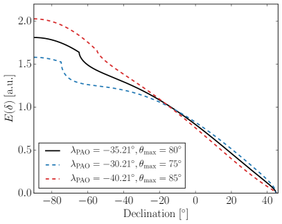
Figure 5: Declination dependence of PAO exposure (black). The two dashed lines show alternative choices of parameters we use to investigate sensitivity of our results to the details of $E(\delta)$.

References

- Alves Batista et al. (2019) R. Alves Batista et al., Front. Astron. Space Sci. 6, 23 (2019), arXiv:1903.06714 [astro-ph.HE] .
- Aab et al. (2017) A. Aab et al. (Pierre Auger), Science 357, 1266 (2017), arXiv:1709.07321 [astro-ph.HE] .
- Abbasi et al. (2014) R. Abbasi et al. (Telescope Array), Astrophys. J. Lett. 790, L21 (2014), arXiv:1404.5890 [astro-ph.HE] .
- Aab et al. (2018) A. Aab et al. (Pierre Auger), Astrophys. J. Lett. 853, L29 (2018), arXiv:1801.06160 [astro-ph.HE] .
- Kashti and Waxman (2008) T. Kashti and E. Waxman, JCAP 05, 006 (2008), arXiv:0801.4516 [astro-ph] .
- Koers and Tinyakov (2009) H. B. Koers and P. Tinyakov, JCAP 04, 003 (2009), arXiv:0812.0860 [astro-ph] .
- di Matteo et al. (2018) A. di Matteo, O. Deligny, K. Kawata, R. M. de Almeida, M. Mostafá, E. Moura Santos, H. Sagawa, P. Tinyakov, I. Tkachev, and N. Toshiyuki, JPS Conf. Proc. 19, 011020 (2018).
- di Matteo et al. (2020) A. di Matteo et al. (Pierre Auger, Telescope Array), PoS ICRC2019, 439 (2020), arXiv:2001.01864 [astro-ph.HE] .
- Abbasi et al. (2018a) R. Abbasi et al. (Telescope Array), Astrophys. J. Lett. 867, L27 (2018a), arXiv:1809.01573 [astro-ph.HE] .
- Tinyakov (2018) P. Tinyakov (Telescope Array), JPS Conf. Proc. 19, 011019 (2018).
- Oikonomou et al. (2013) F. Oikonomou, A. Connolly, F. B. Abdalla, O. Lahav, S. A. Thomas, D. Waters, and E. Waxman, JCAP 05, 015 (2013), arXiv:1207.4043 [astro-ph.HE] .
- Aab et al. (2015a) A. Aab et al. (Pierre Auger), Astrophys. J. 804, 15 (2015a), arXiv:1411.6111 [astro-ph.HE] .
- Abbasi et al. (2018b) R. Abbasi et al. (Telescope Array), Astrophys. J. 862, 91 (2018b), arXiv:1802.05003 [astro-ph.HE] .
- Denton and Weiler (2015) P. B. Denton and T. J. Weiler, Astrophys. J. 802, 25 (2015), arXiv:1409.0883 [astro-ph.HE] .
- Ahlers et al. (2018) M. Ahlers, P. Denton, and M. Rameez, PoS ICRC2017, 282 (2018).
- Urban et al. (2020) F. R. Urban, S. Camera, and D. Alonso, (2020), arXiv:2005.00244 [astro-ph.HE] .
- Aab et al. (2015b) A. Aab et al. (Pierre Auger), Nucl. Instrum. Meth. A 798, 172 (2015b), arXiv:1502.01323 [astro-ph.IM] .
- Huchra et al. (2012) J. P. Huchra et al., Astrophys. J. Suppl. 199, 26 (2012), arXiv:1108.0669 [astro-ph.CO] .
- Gorski et al. (2005) K. Gorski, E. Hivon, A. Banday, B. Wandelt, F. Hansen, M. Reinecke, and M. Bartelman, Astrophys. J. 622, 759 (2005), arXiv:astro-ph/0409513 .
- Hivon et al. (2002) E. Hivon, K. Gorski, C. Netterfield, B. Crill, S. Prunet, and F. Hansen, Astrophys. J. 567, 2 (2002), arXiv:astro-ph/0105302 .
- Chon et al. (2004) G. Chon, A. Challinor, S. Prunet, E. Hivon, and I. Szapudi, Mon. Not. Roy. Astron. Soc. 350, 914 (2004), arXiv:astro-ph/0303414 .
- Ando et al. (2018) S. Ando, A. Benoit-Lévy, and E. Komatsu, Mon. Not. Roy. Astron. Soc. 473, 4318 (2018), arXiv:1706.05422 [astro-ph.CO] .