Fast variable density node generation on parametric surfaces with application to mesh-free methods

Abstract

Domain discretization is considered a dominant part of solution procedures for solving partial differential equations. It is widely accepted that mesh generation is among the most cumbersome parts of the FEM analysis and often requires human assistance, especially in complex 3D geometries. When using alternative mesh-free approaches, the problem of mesh generation is simplified to the problem of positioning nodes, a much simpler task, though still not trivial. In this paper we present an algorithm for generation of nodes on arbitrary $d$-dimensional surfaces. This algorithm complements a recently published algorithm for generation of nodes in domain interiors, and represents another step towards a fully automated dimension-independent solution procedure for solving partial differential equations. The proposed algorithm generates nodes with variable density on surfaces parameterized over arbitrary parametric domains in a dimension-independent way in $O(N\log N)$ time. It is also compared with existing algorithms for generation of surface nodes for mesh-free methods in terms of quality and execution time.

65D99, 65N99, 65Y20, 68Q25

1 Introduction

Generation of nodes on surfaces and their enclosed volumes has many application in different fields of science and engineering, ranging from computer graphics, particularly rendering [3], to mesh-free numerical analysis of partial differential equations (PDEs) [25]. In general, specific applications require specific properties of generated nodes, e.g. for dithering in computer graphics a blue noise distribution is often desired [3], while in mesh-free numerical analysis nodes have to be positioned regularly enough to support stable numerical approximation of differential operators [25]. In the context of mesh-free analysis positioning algorithms have been developed and tested with different mesh-free numerical methods [11, 17, 23, 25, 30]. However, the treatment of boundaries, i.e. discretization of surfaces, has often been overlooked, obtained ad-hoc, or with algorithms for generation of surface meshes, which are needed in mesh based methods. Such approach is conceptually flawed as the whole point of mesh-free methods is to completely remove meshing from the procedure. Furthermore, it is also computationally inefficient, as surface mesh generation algorithms, such as [24] and [18], spend a great deal of time generating connectivity relations, only for those relations to be discarded later. This inefficiencies and increased demand for node generation on surfaces encourage researches to developed specialized algorithms.

Existing algorithms for point generation on parametric surfaces use different techniques, which are often generalizations of algorithms for spatial node generation. The most straightforward is the naive sampling, which generates parametric points in the parametric space, and then maps the points to the surface without any additional processing. Such approach inherently results in a non-uniform and distorted distribution. To avoid distortions, conformal mappings can be a promising option [11], if they are easily available for the surface and if the node placing algorithm in the parametric space supports variable spacing. Original spatial density can be scaled by square root of the Gramian of the parametric map to account for the non-uniformity caused by the map. If not analytically available, conformal mappings can be computed numerically [12], but the computation is expensive and not worth it, in general. For specific surfaces, such as spheres or tori, there are simpler specialized algorithms for point generation [14]. For general surfaces, probabilistic approaches are available [7, 16] which generate uniformly distributed points, but they are often not suitable as node generators for PDE discretization due to the potentially high irregularity. However, both naive and probabilistic approaches can be useful to generate initial distributions for iterative discretization generation schemes, such as minimal energy nodes [15], energy functional minimization [28] or via dynamic simulation with attractive/repulsive forces [24, 17], which are also commonly used in graphics community for various purposes, such as texture generation [27]. Another approach to surface node generation was presented in the paper by Shankar, Kirby and Fogelson [23], which presents surface reconstruction, surface node generation and spatial node generation algorithms. The algorithms were used to obtain discretizations suitable for strong form mesh-free methods, and the surface node generation technique they used is called supersampling-decimation, which samples the parametric space with increased density, maps the points and then decimates the mapped points to conform to the required nodal spacing.

Existing algorithms for node generation on curved surfaces have their shortcomings. Algorithms based on conformal maps are practical only for specific classes of surfaces, probabilistic algorithms usually do not produce distributions of sufficient quality and iterative schemes are needed to improve them, making them less efficient. The naive and supersampling-decimation approaches have their benefits in simplicity and speed in some cases, but the published version in [23] only deals with cases where the surface is homeomorphic to a sphere $\mathbb{S}^{1}$ or $\mathbb{S}^{2}$, parametric domain is a rectangle and nodal spacing is constant. In this paper we present an algorithm for discretization of surfaces that works in arbitrary dimensions with variable nodal spacing, with irregular surfaces and parametric domains, but at the cost of requesting the user to supply the Jacobian $\nabla\boldsymbol{r}$ of the surface map. It has guaranteed $O(N\log N)$ time complexity regardless of the domain shape and nodal spacing and the running time is comparable to published algorithms

The rest of the paper is organized as follows. The proposed surface node placing algorithm is presented in Section 2 along with possible generalizations, the comparison with existing surface placing algorithms is presented in Section 3, its use in meshless numerical simulations is presented in Section 4 and conclusions are presented in Section 5.

2 Node generation algorithm

Boundaries of computational domains can be represented in different forms. Most common ones are as parametrizations (possibly split into patches), such as produced with non-uniform rational B-splines (NURBS) [22] or Radial Basis Functions (RBFs) [4], as level-sets [31] or as subdivision surfaces [19]. Different representations have different desirable and undesirable properties, as discussed in e.g. [26]. We will assume that a parametric representation of the boundary in question is given as $\boldsymbol{r}\colon\Xi\subset\mathbb{R}^{d_{\Xi}}\to\partial\Omega\subset\mathbb{R}^{d}$, along with the Jacobian $\nabla\boldsymbol{r}$. Most of the algorithms described in the introduction also work with parametric representations, and a way to construct them is also offered in [23]. Some surface quantities obtained from higher order derivatives, such as curvature, may also be required to solve PDEs, but they will not be used during node generation. The elements of parametric space $\Xi$ will be called parameters, and the elements of target space $\partial\Omega$ will be called points or nodes, when specific emphasis on discretization is desired. Usually, the dimension $d_{\Xi}$ will be $d-1$, but as described in Section 2.2 this is not a requirement.

Given a nodal spacing function $h\colon\partial\Omega\subset\mathbb{R}^{d}\to(0,\infty)$, we wish to place nodes on $\partial\Omega$, such that spacing around node $\boldsymbol{p}\in\partial\Omega$ is approximately equal to $h(\boldsymbol{p})$.

The proposed node placing algorithm takes a regular parametrization $\boldsymbol{r}$, its Jacobian $\nabla\boldsymbol{r}$, a nodal spacing function $h$ and a set of “seed parameters” $\mathcal{X}$ from $\Xi$ as input. If no seed parameters are supplied by the user, the algorithm chooses a random starting parameter inside $\Xi$. It returns a set of regularly distributed nodes on the surface $\partial\Omega$, conforming to the spacing function $h$.

The node spacing does not take place directly in the target space $\mathbb{R}^{d}$. Instead, we place parameters in the parametric space $\Xi$ using the same principle as for spatial node placing. However, the distance between two parameters $\boldsymbol{\xi}_{1}$ and $\boldsymbol{\xi}_{2}$ is not chosen to be local spacing $h$ but is instead computed in such a way, that the distance between points $\boldsymbol{r}(\boldsymbol{\xi}_{1})$ and $\boldsymbol{r}(\boldsymbol{\xi}_{2})$ is approximately $h$. A spatial search structure of points in $\mathbb{R}^{d}$ is maintained to check for proximity violations.

The node placing algorithm processes nodes sequentially. Initially, seed parameters are put in a queue and their corresponding points in the spatial search structure. In each iteration, a parameter $\boldsymbol{\xi}_{i}$ is dequeued, and expanded into a set of candidate parameters $H_{i}$, by generating a set of directions, represented by unit vectors $\vec{s}_{i,j}$ that approximately uniformly cover all possible spatial directions in $\Xi$.

To derive how far from $\boldsymbol{\xi}_{i}$ a candidate parameter must be placed to achieve appropriate distance between points, we consider a candidate parameter $\boldsymbol{\eta}_{i,j}\in H_{i}$ in the direction $\vec{s}_{i,j}$ from $\boldsymbol{\xi}_{i}$,

(1) $$\boldsymbol{\eta}_{i,j}=\boldsymbol{\xi}_{i}+\alpha_{i,j}\vec{s}_{i,j},$$

for some distance $\alpha_{i,j}>0$. Denote the point corresponding to $\boldsymbol{\xi}_{i}$ as $\boldsymbol{p}_{i}=\boldsymbol{r}(\boldsymbol{\xi}_{i})$. We would like the distance between the candidate point $\boldsymbol{r}(\boldsymbol{\eta}_{i,j})$ and $\boldsymbol{p}_{i}$ in $\partial\Omega$ to be equal to $h(\boldsymbol{p}_{i})$

(2) $$\|\boldsymbol{r}(\boldsymbol{\eta}_{i,j})-\boldsymbol{r}(\boldsymbol{\xi}_{i})\|=h(\boldsymbol{p}_{i}),$$

where $\|\cdot\|$ is the standard Euclidean distance. Using first order Taylor’s expansion, we write

(3) $$\boldsymbol{r}(\boldsymbol{\eta}_{i,j})=\boldsymbol{r}(\boldsymbol{\xi}_{i}+\alpha_{i,j}\vec{s}_{i,j})\approx\boldsymbol{r}(\boldsymbol{\xi}_{i})+\alpha_{i,j}\nabla\boldsymbol{r}(\boldsymbol{\xi}_{i})\vec{s}_{i,j}.$$

Substituting the linear approximation (3) in (2), we obtain an equation for $\alpha_{i,j}$ as

(4) $$h(\boldsymbol{p}_{i})=\|\boldsymbol{r}(\boldsymbol{\xi}_{i})+\alpha_{i,j}\nabla\boldsymbol{r}(\boldsymbol{\xi}_{i})\vec{s}-\boldsymbol{r}(\boldsymbol{\xi}_{i})\|=\alpha_{i,j}\|\nabla\boldsymbol{r}(\boldsymbol{\xi}_{i})\vec{s}_{i,j}\|,$$

where we took into account the positivity of $\alpha_{i,j}$. This equation is solved for $\alpha_{i,j}$ to obtain the candidate parameter

(5) $$\boldsymbol{\eta}_{i,j}=\boldsymbol{\xi}_{i}+\frac{h(\boldsymbol{p}_{i})}{\|\nabla\boldsymbol{r}(\boldsymbol{\xi}_{i})\vec{s}_{i,j}\|}\vec{s}_{i,j},\quad\alpha_{i,j}=\frac{h(\boldsymbol{p}_{i})}{\|\nabla\boldsymbol{r}(\boldsymbol{\xi}_{i})\vec{s}_{i,j}\|}.$$

Higher order terms of the approximation could be used in (3), but the equation (4) would also be of higher order and higher derivatives of $\boldsymbol{r}$ would be required.

The set of candidates $H_{i}$ is generated from directions $\vec{s}_{i,j}$ as

(6) $$H_{i}=\left\{\boldsymbol{\xi}_{i}+\frac{h(\boldsymbol{p}_{i})}{\|\nabla\boldsymbol{r}(\boldsymbol{\xi}_{i})\vec{s}_{i,j}\|}\vec{s}_{i,j}\mid\vec{s}_{i,j}\in\text{directions}(\boldsymbol{\xi}_{i})\right\}.$$

Candidate parameters that lie outside of the parametric space $\Xi$ are discarded. Additionally, candidate parameters whose corresponding points lie too close to already accepted points are also rejected. The remaining candidate parameters are enqueued for expansion and their corresponding points are added to the spatial search structure.

When checking the distance from a candidate point to its closest already existing point, the algorithm compares the found distance with $\|\boldsymbol{r}(\boldsymbol{\eta}_{i,j})-\boldsymbol{r}(\boldsymbol{\xi}_{i})\|=:\hat{h}_{i,j}$ instead of $h(\boldsymbol{p}_{i})$. Unless this adjustment is made, no candidates would be accepted in areas where $\hat{h}_{i,j}$ is smaller than $h(\boldsymbol{p})$, since point $\boldsymbol{p}_{i}$ itself would be too close. On curves, this might even cause the algorithm to terminate prematurely.

Figure 1 illustrates the process of candidate generation on a surface parameterized with $\boldsymbol{r}(\xi_{1},\xi_{2})=(\xi_{1},\xi_{2},3\sin\xi_{1}\sin\xi_{2})$. Parameters in parametric space $\Xi$ (left) are generated in a way that when mapped to the main domain $\partial\Omega$ (right), they are approximately $h$ apart.

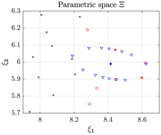
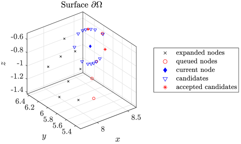
Figure 1: Illustration of candidate generation by the proposed algorithm in parametric space $\Xi$ (left) and main domain $\partial\Omega$ (top), around parameter $\boldsymbol{\xi}=(8.42,5.99)$ with spacing $h=0.23$.

Figure 2 illustrates the execution of the proposed algorithm on a part of a unit sphere (non-standardly) parameterized by $\boldsymbol{r}(\xi_{1},\xi_{2})=(\cos\xi_{1}\sin\xi_{2}^{2},\sin\xi_{1}\sin\xi_{2}^{2},\cos\xi_{2}^{2})$ with a constant nodal spacing. The algorithm begins with a single node (leftmost image) and then expands it in all directions. Subsequent images show progress of the proposed algorithm and the final result (rightmost image).

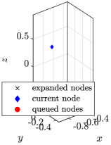
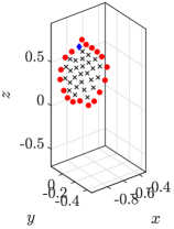
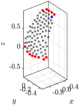
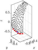
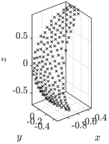
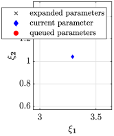
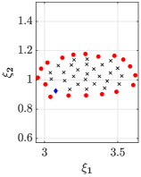
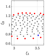
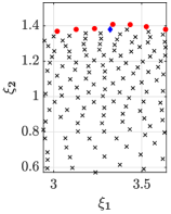
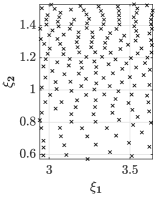
Figure 2: Execution illustration of the proposed algorithm algorithm (left to right) in parametric domain $\Xi$ (bottom) and main domain $\partial\Omega$ (top). Part of a unit sphere was sampled with nodal spacing $h=0.08$.

An efficient implementation with an implicit queue contained in the array of final points and the $k$-d tree spatial structure [21] is presented as Algorithm 1.

Algorithm 1 Proposed surface node placing algorithm.

Input: Parametric domain $\Xi\subseteq\mathbb{R}^{d_{\Xi}}$, given by its characteristic function $\chi_{\Xi}\colon\mathbb{R}^{d_{\Xi}}\to\{0,1\}$.
Input: Parametrization $\boldsymbol{r}\colon\Xi\to\partial\Omega\subset\mathbb{R}^{d}$ and its Jacobian matrix $\nabla\boldsymbol{r}$.
Input: A list of starting parameters $\mathcal{X}$ from the parametric domain $\Xi$.
Input: A nodal spacing function $h\colon\partial\Omega\subset\mathbb{R}^{d}\to(0,\infty)$.
Input: Number of candidates generated in each iteration $n$.
Output: A list of points in $\partial\Omega$ distributed according to spacing function $h$.

1:function proposedAlgorithm($\Xi,\boldsymbol{r},\nabla\boldsymbol{r},h,\mathcal{X},n$)

2:    $T\leftarrow\textsc{kdtreeInit}(\boldsymbol{r}(\mathcal{X}))$ $\triangleright$ Initialize spatial search structure on points $\boldsymbol{r}(\mathcal{X})$.

3:    $i\leftarrow 0$ $\triangleright$ Current node index.

4:    while $i<|\mathcal{X}|$ do $\triangleright$ Until the queue is not empty.

5:         $\boldsymbol{\xi}_{i}\leftarrow\mathcal{X}[i]$ $\triangleright$ Get next parameter values from the start of the queue.

6:         $\boldsymbol{p}_{i}\leftarrow\boldsymbol{r}(\boldsymbol{\xi}_{i})$ $\triangleright$ Compute the corresponding node in $\partial\Omega$.

7:         $h_{i}\leftarrow h(\boldsymbol{p}_{i})$ $\triangleright$ Compute its nodal spacing.

8:         for each $\vec{s}_{i,j}$ in candidates($n$) do $\triangleright$ Loop through random unit vectors.

9:             $\boldsymbol{\eta}_{i,j}\leftarrow\boldsymbol{\xi}_{i}+\frac{h_{i}}{\|\nabla\boldsymbol{r}(\boldsymbol{\xi}_{i})\vec{s}_{i,j}\|}\vec{s}_{i,j}$ $\triangleright$ Calculate new candidate.

10:             if $\boldsymbol{\eta}_{i,j}\in\Xi$ then $\triangleright$ Discard candidates outside the parametric domain.

11:                 $\boldsymbol{c}_{i,j}\leftarrow\boldsymbol{r}(\boldsymbol{\eta}_{i,j})$ $\triangleright$ Compute the candidate point in $\partial\Omega$.

12:                 $\hat{h}_{i,j}\leftarrow\|\boldsymbol{c}_{i,j}-\boldsymbol{p}_{i,j}\|$ $\triangleright$ Compute the actual spacing.

13:                 $\boldsymbol{n}_{i,j}\leftarrow\textsc{kdtreeClosest}(T,\boldsymbol{c}_{i,j})$ $\triangleright$ Find nearest node for proximity test.

14:                 if $\|\boldsymbol{c}_{i,j}-\boldsymbol{n}_{i,j}\|\geq\hat{h}_{i,j}$ then $\triangleright$ Test that $\boldsymbol{c}_{i,j}$ is not too close to other nodes.

15:                     append($\mathcal{X},\boldsymbol{\eta}_{i,j}$) $\triangleright$ Enqueue $\boldsymbol{\eta}_{i,j}$ as the last element of $\mathcal{X}$.

16:                     kdtreeInsert($T,\boldsymbol{c}_{i,j}$) $\triangleright$ Insert $\boldsymbol{c}_{i,j}$ into the spatial search structure.

17:                 end if

18:             end if

19:         end for

20:         $i\leftarrow i+1$ $\triangleright$ Dequeue current parameter and move to the next one.

21:    end while

22:    return $\boldsymbol{r}(\mathcal{X})$

23:end function

The proposed algorithm includes generation of random unit direction vectors on line 8, that needs to be clarified. There are different ways of generating unit vectors that cover all possible directions well, according to discussion in [25], randomized pattern candidates technique shall be used. A set of random unit vectors is obtained by randomly rotating a fixed discretization of a $d$-dimensional unit ball. The set of candidates $\textsc{candidates}(n)$ on a unit ball in 2D is obtained simply by

(7) $$\textsc{candidates}(n)=\left\{(\cos\varphi,\sin\varphi);\ \varphi\in\{0,\varphi_{0},2\varphi_{0},\ldots,(n-1)\varphi_{0}\},\varphi_{0}=\frac{2\pi}{n}\right\}.$$

In $d$ dimensions, the discretization of a unit ball is obtained by recursively discretizing appropriate $d-1$ dimensional slices along the last coordinate.

The number of generated candidates $n$ in each iteration on line 8 is also a free parameter in our implementation of the proposed algorithm and recommendations based on the dimension $d_{\Xi}$ are given in [25]. We will use $n=2$ when $d_{\Xi}=1$ and $n=15$ when $d_{\Xi}=2$ in our analyses, unless stated otherwise.

2.1 Time complexity analysis

We will derive the time complexity in terms of the number of generated nodes. Let us denote the number of starting points with $N_{s}$, the number of final points with $N$, the cost of spatial search structure precomputation, query and insertion with $P(N_{s}),Q(N)$ and $I(N)$ respectively, the cost of evaluating $\boldsymbol{r}$ with $e_{1}$ and the cost of evaluating $\nabla\boldsymbol{r}$ with $e_{2}$. All other operations are assumed to have (amortized) constant cost.

The main while loop (line 4) iterates exactly $N$ times and the inner for loop (line 8) iterates $n$ times. Each iteration of the inner for loop executes one query and one $\boldsymbol{r}$ evaluation. Every candidate was inserted once and $\nabla\boldsymbol{r}$ is evaluated once for each node when expanding it, since its value can be stored for later use in the inner for loop. Therefore, the total time complexity of the proposed algorithm is equal to

(8) $$T_{\text{PA-general}} =P(N_{s})+\sum_{i=1}^{N}(I(N)+e_{1}+e_{2}+\sum_{j=1}^{n}(e_{1}+Q(N)))$$

$$=O(P(N_{s})+N(n+1)e_{1}+Ne_{2}+NnQ(N)+NI(N)).$$

Since we are using a $k$-d tree as the spatial search structure, we know that $P(N_{s})=O(N_{s}\log N_{s}),Q(N)=O(\log N)$ and $I(N)=O(\log N)$. Both $e_{1}$ and $e_{2}$ are also usually constant cost operations and $N_{s}=O(N)$ (usually even $N_{s}\ll N$). This simplifies equation (8) to

(9) $$T_{\text{PA}}=O(N_{s}\log N_{s}+nN+nN\log N)=O(nN\log N).$$

Other data structures can be used in special cases. If $h$ is constant, a background grid with spacing $O(h/\sqrt{d})$ can be faster, but less space efficient, supporting query and insert operations in $O(1)$. Additionally, when when sampling simple curves from a single starting point, the search structure is unnecessary as the parameters are sampled in the interval and we can simply advance in both directions and the only conflict can appear when the two ends of the curve potentially meet.

In this article, we will be using the general $k$-d tree version of the algorithm unless stated otherwise explicitly.

2.2 Remarks on generalizations

In general, the parametrization function $\boldsymbol{r}$ does not need to map to a smooth boundary $\partial\Omega$ of a domain $\Omega$. However, having orientability and co-dimension one allows the algorithm to also uniquely generate unit normals from $\nabla\boldsymbol{r}$. Normal generation aside, neither orientability nor co-dimension are requirements for the algorithm. The algorithms works in exactly the same manner if $d_{\Xi}<d-1$, e.g. for a curve embedded in 3D space.

Additionally, there are also no problems with self-intersecting surfaces. As an example of that, the discretization of the (non-orientable) Roman surface is shown in Fig. 3. The Roman surface is a mapping of the real projective plane $\mathbb{R}\textup{P}^{2}$ in $\mathbb{R}^{3}$, given by

(10) $$\boldsymbol{r}(\theta,\varphi)=(R^{2}\cos\theta\sin\theta\sin\varphi,R^{2}\cos\theta\sin\theta\cos\varphi,R^{2}\cos^{2}\theta\cos\varphi\sin\varphi).$$

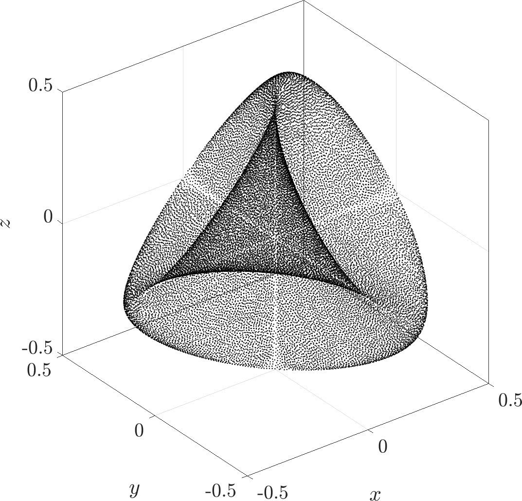
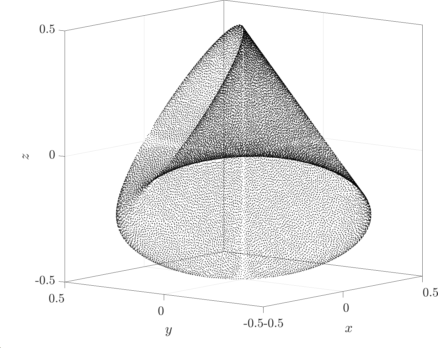
Figure 3: Nodes generated by the proposed algorithm on the Roman surface (10) with $R=1,h=0.005$.

Although all examples in this paper only deal with closed surfaces, the generalization to bounded surfaces is straightforward. First, the boundary is to be discretized, using the proposed algorithm, followed by discretization of remaining of the surface using the generated boundary nodes as seed nodes.

There is also a possibility to extend the algorithm to surfaces defined by multiple possibly intersecting patches, such as models created by Computer aided design (CAD) software or parameterized submanifolds. The algorithm can discretize the surface patch by patch and the spatial search structure keeps all the information about stored nodes from the previous patches, to check for spacing violations. Problems might arise on patch joints, similarly to front-joints, which could be dealt with post-process algorithms [17]. However, further discussion on this topic is out of scope of this paper and is left for future work.

3 Discussion and comparison

The proposed algorithm is compared with the supersampling-decimation technique, recently published by Shankar, Kirby and Fogelson [23], and the naive sampling algorithm, which was also used in [23] to show the significance of the supersampling-decimation technique. A brief description of both algorithms follows, using the same notation as in Section 2. When needed, we will refer to the naive algorithm as NA, to the supersampling-decimation approach as SD and to the proposed algorithm as PA.

3.1 Existing algorithms

3.1.1 Naive parametric sampling

Naive parametric sampling attempts to generate a discretization of a surface parameterized with $\boldsymbol{r}\colon\Xi\subset\mathbb{R}^{d_{\Xi}}\to\partial\Omega\subset\mathbb{R}^{d}$, by discretizing $\Xi$ with nodal spacing $h$, obtaining a set of parameters $\mathcal{X}_{\Xi}$. The discretization points are obtained by simply mapping elements of $\mathcal{X}_{\Xi}$ to the surface, i.e. the resulting set of points $\mathcal{X}$ is given by $\mathcal{X}=\boldsymbol{r}(\mathcal{X}_{\Xi})$.

This type of sampling is useful for its simplicity, especially if $\Xi$ is box-shaped, $h$ constant and gradients $\nabla\boldsymbol{r}$ are not too large. The algorithm is included in this paper mostly as a reference to put results in perspective.

3.1.2 Supersampling-decimation

The supersampling algorithm is based on the naive algorithm, except that the discretization of the parametric space $\Xi$ uses spacing $h_{\Xi}:=h/\gamma$ instead of $h$, where $\gamma>0$ is called the supersampling factor. This is done in order to generate enough nodes even where the mapping $\boldsymbol{r}$ might cause them to spread out on the surface. After the set of parameters $\mathcal{X}_{\Xi}$ with spacing $h/\gamma$ has been generated, decimation or thinning is performed, to keep only the appropriate nodes. The parameters are mapped to the surface in sequence, accepting only the points that are not too close to already accepted ones. This requires the use of a spatial search structure that supports ball queries. The end result is a set of nodes $\mathcal{X}$ in $\partial\Omega$, that are spaced approximately by $h$.

The algorithm as described in [23] assumes that $\Xi$ is either a line or a rectangle and that spacing $h$ is constant. Additionally, $\gamma$ is not chosen directly, but indirectly by estimating the number of nodes $N$ on the generated surface as $N=|\partial\Omega|/h^{d}$ and generating $\tau N$ of them, with spacing $h_{\mathcal{X}}=\sqrt[d_{\Xi}]{|\Xi|/(\tau N)}=h\sqrt[d_{\Xi}]{|\Xi|/(\tau|\partial\Omega|)}$, effectively choosing $\gamma=\sqrt[d_{\Xi}]{\tau|\partial\Omega|/|\Xi|}$. As $|\partial\Omega|$ is not known directly, is is estimated with the surface of an (oriented) bounding box of $\Omega$.

We will similarly take into the account the scaling due to different surface areas, but will scale $h$ directly by $\tau$, using $\gamma=\tau\sqrt[d_{\Xi}]{|\partial\Omega|/|\Xi|}$. Value $\tau=5$ will be sufficient in most cases and will be used unless otherwise specified.

3.2 Setup for comparison

In this paper we focus on generating nodes for use in meshless numerical analysis and therefore all analyses are done with guidelines established in [25] in mind. These include local regularity, minimal spacing requirements, computational efficiency and the number of tuning parameters. In the following discussion we analyze algorithm presented in Section 2 and compare it to the naive and supersampling algorithms.

In most of the analyses we will use a polar curve used in [23], given by

(11) $$r_{p}(\varphi)=|\cos(1.5\varphi)|^{\sin(3\varphi)},\quad\boldsymbol{r}_{p}(\varphi)=(r_{p}(\varphi)\cos\varphi,r_{p}(\varphi)\sin\varphi),\quad\varphi\in[0,2\pi)$$

and a heart-like surface in 3D, given by

(12) $$\boldsymbol{r}_{h}(u,v)=(\sqrt{1-v^{2}}\cos(u)+v^{2},\sqrt{1-v^{2}}\sin(u),v),\quad(u,v)\in[0,2\pi)\times[-1,1).$$

Both of these parametrizations have large variations in absolute value of partial derivatives, which makes them good candidates for analyses.

All three algorithms were implemented in C++ using the same library for $k$-d tree spatial search structure (nanoflann [2]) and the same linear algebra library (Eigen [13]) to ensure as fair comparison as possible. This implementation of the proposed algorithm is included in the Medusa library [20], a C++ library focused on tools for solving Partial Differential Equations with strong-form meshless methods. Its standalone C++ implementation is also available at [8].

3.3 Local regularity

We begin our analysis by visually comparing the node sets, generated with different algorithms. In Fig. 4 we can see their performance on the polar curve $\boldsymbol{r}_{p}$. It is clear that the naive algorithm does not perform well on curves with variable derivatives. We can also see some irregularly big gaps between nodes generated by the supersampling algorithm, since the supersampling algorithm is based on the naive algorithm. However, this can be improved by choosing a bigger value of the supersampling parameter $\tau$, at greater cost to execution time and memory. Nodes generated by the proposed algorithm only have one visually bigger gap, where two sides of the parametric domain meet.

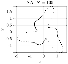
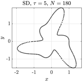
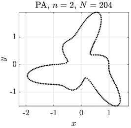
Figure 4: Comparison of different algorithms on a 2D polar curve from (11) sampled with $h=0.06$

In Fig. 5 we can see their performance in 3D on the heart-like surface $\boldsymbol{r}_{h}$. Naive algorithm’s performance is similarly poor as in 2D case. Nodes generated by the supersampling algorithm have bigger gaps only around $(1,0,1)$ and $(1,0,-1)$, where partial derivatives of $\boldsymbol{r}_{h}$ diverge. In the same way as in the 2D case, increasing $\tau$ gives better results, but the increase must be dependent on $h$ to achieve good quality in all cases. The proposed algorithm also performs worse near those points. However, it can handle such problematic areas automatically and provides stable results regardless the $h$. A more in-depth analysis of minimal and maximal spacing for various $h$ is presented in Section 3.4.

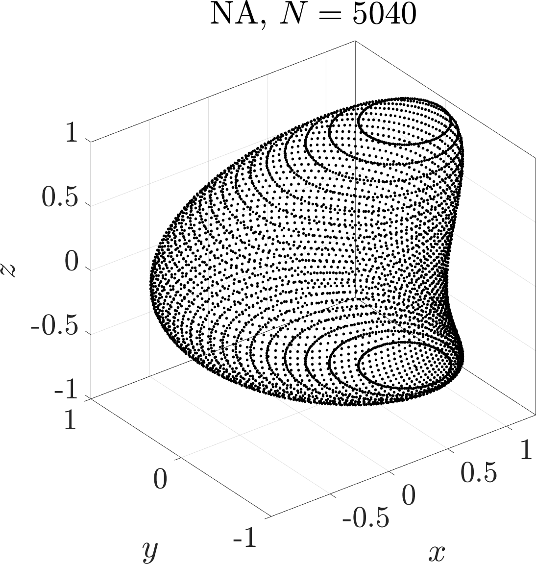
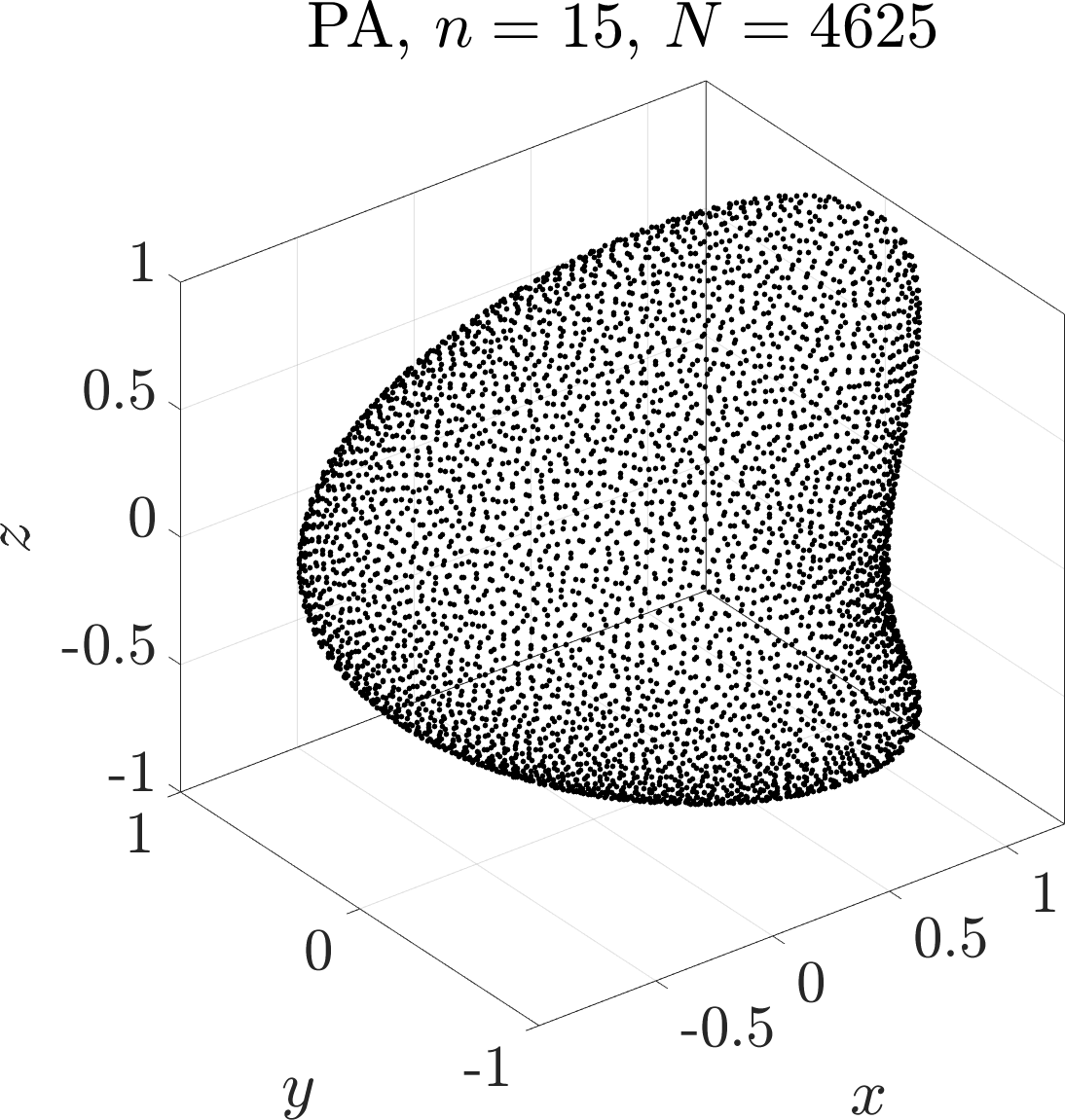
Figure 5: Comparison of different algorithms on a 3D heart-like surface from (12) sampled with $h=0.05$

To further analyze local regularity, we examine the distribution of distances to nearest neighbors. For each node $\boldsymbol{p}_{i}$ we find $c$ nearest neighbors $\boldsymbol{p}_{i,j},j=1,2,\dots c$ and calculate the average distance between them $\bar{d}_{i}=\frac{1}{c}\sum_{j=1}^{c}\|\boldsymbol{p}_{i}-\boldsymbol{p}_{i,j}\|$. We also calculate the maximum and minimum distances for each point, $d_{i}^{\text{min}}$ and $d_{i}^{\text{max}}$, where

(13) $$d_{i}^{\text{min}}=\min_{j=1,\dots c}\|\boldsymbol{p}_{i}-\boldsymbol{p}_{i,j}\|,\qquad d_{i}^{\text{max}}=\max_{j=1,\dots c}\|\boldsymbol{p}_{i}-\boldsymbol{p}_{i,j}\|.$$

with $c=2$ for $d_{\Xi}=1$ and $c=3$ for $d_{\Xi}=2$. The results are presented in terms of normalized distances ($\bar{d}^{\prime}$, $(d_{i}^{\text{min}})^{\prime}$, etc.) which are scaled by $h$, e.g.

(14) $$\bar{d}^{\prime}=\bar{d}/h.$$

Numerical results of this analysis are shown in Table 1.

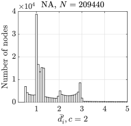
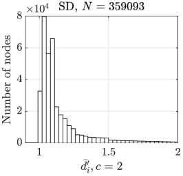
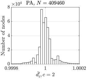
Figure 6: Histogram of normalized average distances to 2 nearest neighbors a polar curve from (11) sampled with $h=0.00003$. $\tau=5,n=2$. Note the different scaling on the horizontal axes.

Figure 6 shows the distribution of normalized average distances for 2 nearest neighbors on the polar curve. The supersampling algorithm and the proposed algorithm perform much better than the naive algorithm, with distribution of nodes generated by the proposed algorithm being of higher quality. The proposed algorithm produces distribution with normalized mean distance much closer to the target value $1$ in comparison to the supersampling algorithm. Furthermore, the standard deviation of $\bar{d}^{\prime}$ of nodes generated by the proposed algorithm is a few orders of magnitude smaller than the standard deviation of $\bar{d}^{\prime}$ of nodes generated by the supersampling algorithm (see Table 1). Both algorithms show similar mean difference between the maximum and minimum distance, with the supersampling algorithm performing slightly better in this aspect.

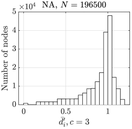
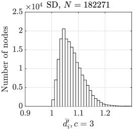
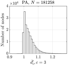
Figure 7: Histogram of normalized average distances to 3 nearest neighbors on a heart-like surface from (12) sampled with $h=0.008$.

Figure 7 shows the same plots for 3 neighbors on the heart-like surface. The results are also similar to the $d_{\Xi}=1$ case, the proposed algorithm has a more favorable mean and standard deviation of $\bar{d}^{\prime}$ than supersampling algorithm, while the naive algorithm is much worse than both of them. However, the differences between the proposed and supersampling algorithms are much smaller than in the previous analysis. It is important to note that increasing the supersampling parameter $\tau$ would, to some degree, improve the results of supersampling, however at greater computational cost.

Table 1: Numerical quantities related to local regularity. 2D polar curve from (11) sampled with $h=0.00003$ and 3D heart-like surface from (12) sampled with $h=0.004$.

case	alg.	$\operatorname{mean}\bar{d}^{\prime}_{i}$	$\operatorname{std}\bar{d}^{\prime}_{i}$	$\operatorname{mean}\left(\left(d_{i}^{\text{max}}\right)^{\prime}-\left(d_{i}^{\text{min}}\right)^{\prime}\right)$
$d_{\Xi}=1$	PA	1.0001	$5.1483\times 10^{-4}$	$1.1136\times 10^{-10}$
	SD	1.1403	0.1715	$5.7655\times 10^{-9}$
	NA	1.9550	1.8386	$2.7922\times 10^{-8}$
$d_{\Xi}=2$	PA	1.0357	0.0374	$3.8888\times 10^{-4}$
	SD	1.0764	0.0473	$3.3444\times 10^{-4}$
	NA	0.8946	0.2086	0.0013

A graph of $\bar{d}_{i}^{\prime}$ for each node $\boldsymbol{p}_{i}$ with error bars showing $(d_{i}^{\text{max}})^{\prime}$ and $(d_{i}^{\text{min}})^{\prime}$ is shown in Fig. 8 for the polar curve. From this graph we can see that all three algorithms have degraded performance only on certain points on the curve, where derivatives of $\boldsymbol{r}_{p}$ rapidly increase. Nevertheless, the proposed algorithm handles curves with large derivatives better.

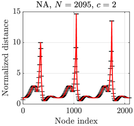
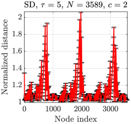
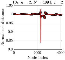
Figure 8: Graph of normalized average distances to 2 nearest neighbors on a 2D polar curve from (11) sampled with $h=0.003$. Error bars show minimal and maximal normalized distances to 2 nearest neighbors. Note the different $y$-axis range in the plots.

Figure 9 shows the same analysis as Fig. 8 for $d_{\Xi}=2$ case. The differences between the supersampling and the proposed algorithm decrease and it can be seen that the supersampling algorithm actually has fewer outliers with high valued $\bar{d}_{i}^{\prime}$ and $(d_{i}^{\text{max}})^{\prime}$ or low valued $(d_{i}^{\text{min}})^{\prime}$.

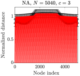
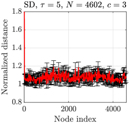
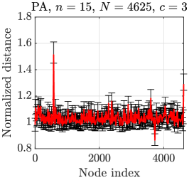
Figure 9: Graph of normalized average distances to 3 nearest neighbors on a 3D heart-like surface from (12) sampled with $h=0.5$. Error bars show minimal and maximal normalized distances to 3 nearest neighbors. Note the different $y$-axis range in the plots.

3.4 Minimal and maximal spacing requirements

Minimal and maximal spacing guarantees are in principle inherited from the underlying algorithm used to discretize $\Xi$, but they are distorted by application of $\boldsymbol{r}$ in the naive algorithm. Supersampling algorithm ensures directly that minimal spacing $h$ is respected in its decimation step. The proposed algorithm uses $\hat{h}_{i,j}$ instead of $h$ to check for distance violations, and this introduces an error caused by using linear Taylor’s approximation. The exact spacing at point $\boldsymbol{p}=r(\boldsymbol{\xi})$ is equal to $h(\boldsymbol{p})$, while the actual computed spacing is equal to $\hat{h}(\boldsymbol{\xi},\vec{s})=\|\boldsymbol{r}(\boldsymbol{\xi}+(h(\boldsymbol{p})/\|\nabla\boldsymbol{r}(\boldsymbol{\xi})\vec{s}\|)\vec{s})-\boldsymbol{r}(\boldsymbol{\xi})\|$. We wish to estimate the error $\Delta h(\boldsymbol{\xi},\vec{s})=h(\boldsymbol{p})-\hat{h}(\boldsymbol{\xi},\vec{s})$, specifically, we would like upper bounds of the form $|\Delta h|\leq M$. Three types of bounds are of interest: where $M$ depends on $\boldsymbol{\xi}$ and $\vec{s}$, where $M$ depends only on $\xi$ and where $M$ is independent and the bound is global.

Proposition 3.1.

The following estimates hold for the error of local node spacing radius due to linear approximation in (3):

(15) $$|\Delta h(\boldsymbol{\xi},\vec{s})| \leq\frac{\sqrt{d_{\Xi}}}{2}h(\boldsymbol{p})^{2}\frac{\displaystyle\max_{i=1,\ldots,d_{\Xi}}\max_{\theta\in[0,\alpha]}\left|\vec{s}^{\mathsf{T}}(\nabla\nabla r_{i})(\boldsymbol{\xi}+\theta\vec{s})\vec{s}\right|}{\|\nabla\boldsymbol{r}(\boldsymbol{\xi})\vec{s}\|^{2}},\alpha=\frac{h(\boldsymbol{p})}{\|\nabla\boldsymbol{r}(\boldsymbol{\xi})\vec{s}\|},$$

(16) $$|\Delta h(\boldsymbol{\xi})| \leq\frac{\sqrt{d_{\Xi}}}{2}h(\boldsymbol{p})^{2}\frac{\displaystyle\max_{i=1,\ldots,d_{\Xi}}\max_{\boldsymbol{\zeta}\in\bar{B}(\boldsymbol{\xi},\rho_{\boldsymbol{\xi}})}\sigma_{1}((\nabla\nabla r_{i})(\boldsymbol{\zeta}))}{\sigma_{d_{\Xi}}(\nabla\boldsymbol{r}(\boldsymbol{\xi}))^{2}},\;\rho_{\boldsymbol{\xi}}=\frac{h(\boldsymbol{p})}{\sigma_{d_{\Xi}}(\nabla\boldsymbol{r}(\boldsymbol{\xi}))},$$

(17) $$|\Delta h| \leq\frac{\sqrt{d_{\Xi}}}{2}h_{M}^{2}\frac{\sigma_{1,M}(\nabla\nabla\boldsymbol{r})}{\sigma_{d_{\Xi},m}^{2}(\nabla\boldsymbol{r})},$$

where

(18) $$h_{M} =\max_{\boldsymbol{\xi}\in\Xi}h(\boldsymbol{p}),$$

(19) $$\sigma_{1,M}(\nabla\nabla\boldsymbol{r}) =\max_{i=1,\ldots,d_{\Xi}}\max_{\boldsymbol{\xi}\in\Xi}\sigma_{1}((\nabla\nabla r_{i})(\boldsymbol{\xi})),$$

(20) $$\sigma_{d_{\Xi},m}(\nabla\boldsymbol{r}) =\min_{\boldsymbol{\xi}\in\Xi}\sigma_{d_{\Xi}}(\nabla\boldsymbol{r}(\boldsymbol{\xi})),$$

and $\sigma_{i}(A)$ denotes the $i$-th largest singular value of $A$.

In particular, this means that the relative error in spacing $|\Delta h|/h$ decreases linearly with $h$ for well behaved $\boldsymbol{r}$ and the algorithm for placing points on surfaces asymptotically retains the minimal spacing and quasi-uniformity bounds of the underlying algorithm for flat space.

Proposition 3.1 tells us that the relative error due to linear approximation when computing $\alpha$ is of order $h$, where the proportionality constant depends on properties of $\nabla\boldsymbol{r}$ and $\nabla\nabla\boldsymbol{r}$. Its proof is given in Appendix A.

To analyze minimal and maximal spacing quantitatively, we can use standard concepts (see e.g. [29, 14]), such as maximum empty sphere radius and separation distance. For a set of points $\mathcal{X}=\{x_{1},\dots,x_{N}\}\subseteq\partial\Omega$, the maximum empty sphere radius is defined as

(21) $$r_{\max,\mathcal{X}}=\sup_{x\in\partial\Omega}\min_{1\leq j\leq N}\|x-x_{j}\|$$

and the separation distance is defined as

(22) $$r_{\min,\mathcal{X}}=\frac{1}{2}\min_{i\neq j}\|x_{i}-x_{j}\|$$

For numerical computation we compute $r_{\min,\mathcal{X}}$ exactly using a spatial search structure, such as a $k$-d tree, and we estimate $r_{\max,\mathcal{X}}$ by discretizing the surface with a much smaller nodal spacing $h$ and finding the maximum empty sphere with center in one of the generated nodes.

According to Proposition 3.1 we conclude that $r_{\min,\mathcal{X}}/h\geq 1+|\Delta h|/h$ for constant $h$. This bound has been tested on a torus parameterized with $\boldsymbol{r}(\xi_{1},\xi_{2})=((\cos\xi_{2}+2)\cos\xi_{1},(\cos\xi_{2}+2)\sin\xi_{1},\sin\xi_{2}),\xi_{1},\xi_{2}\in[0,2\pi]$. By using a computer algebra system, we can calculate that $\sigma_{1,M}(\nabla\nabla\boldsymbol{r})/\sigma_{d_{\Xi},m}^{2}(\nabla\boldsymbol{r})=3$ and compare this with practical results, shown in Fig. 10. We can see that the $r_{\min,\mathcal{X}}$ obeys its lower bound.

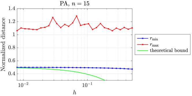
Figure 10: Comparison of practical separation distance and its theoretical lower on nodes generated by the proposed algorithm on a torus in 3D.

Figure 11 shows a graph of maximum empty sphere radius and normalized separation distance of the polar curve $\boldsymbol{r}_{p}$. For the naive and supersampling algorithms, normalized maximum empty sphere radius is increasing with decreasing $h$, because neither of them is able to adapt to the varying value of partial derivatives, and both perform poorly when $\nabla\boldsymbol{r}_{p}$ has high values and when $h$ is smaller. The proposed algorithm scales much better, i.e. $r_{\max}$ remains relatively stable, but does not have a strict separation distance minimum of $0.5$, due to the linear approximation error, as discussed previously.

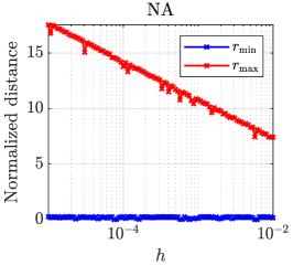
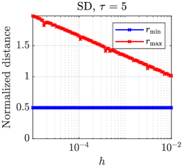
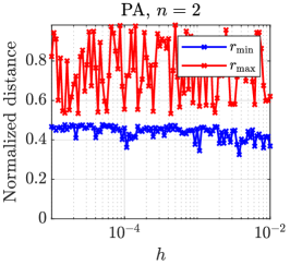
Figure 11: Graph of separation distance and maximum empty sphere radius for different $h$ on the polar curve $\boldsymbol{r}_{p}$ (11). Note the different $y$-axis spans on the plots.

In Fig. 12 we can see the same graph for the heart-like surface $\boldsymbol{r}_{h}$ (12). The results are similar, however $r_{\max}$ is increasing faster and does not seem bounded for nodes generated by the proposed algorithm. The reason is similar to the one in 2D, only in this case, higher order partial derivatives are increasing faster. If this is causing problems, the proposed algorithm can be improved by using higher orders in the Taylor expansion discussed in Section 2. The performance of the supersampling algorithm can also be improved by using the higher value of the supersampling parameter $\tau$, which delays the problem until even smaller $h$. To mitigate this issue, $\tau$ should be appropriately increased every time $h$ is decreased.

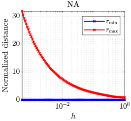
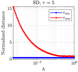
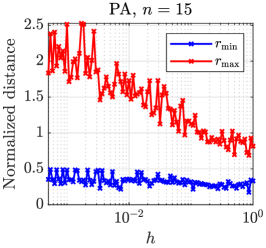
Figure 12: Graph of separation distance and maximum empty sphere radius for different $h$ for the heart-like surface $\boldsymbol{r}_{h}$ (12). Note the different $y$-axis spans on the plots.

3.5 Spatial variability

An important feature of the proposed algorithm, which other algorithms discussed here do not posses, is sampling of parametric surfaces with non-constant spacing functions $h$. As a demonstration, a spherical model of Earth (using the parametrization in spherical coordinates) was sampled by the proposed algorithm, with density function $h$ representing altitudes at different points on Earth. Our implementation of the proposed algorithm has generated $100\,457$ nodes in less than $0.3\,\mathrm{s}$ on an Intel(R) Xeon(R) CPU E5-2620 v3 @ 2.40GHz. The necessary data was acquired from Matlab^®’s topo.mat file, also available from US National Geophysical Data Center [5]. The results can be seen in Fig. 13.

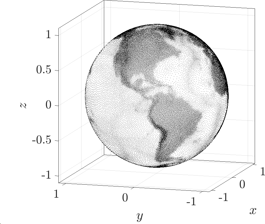
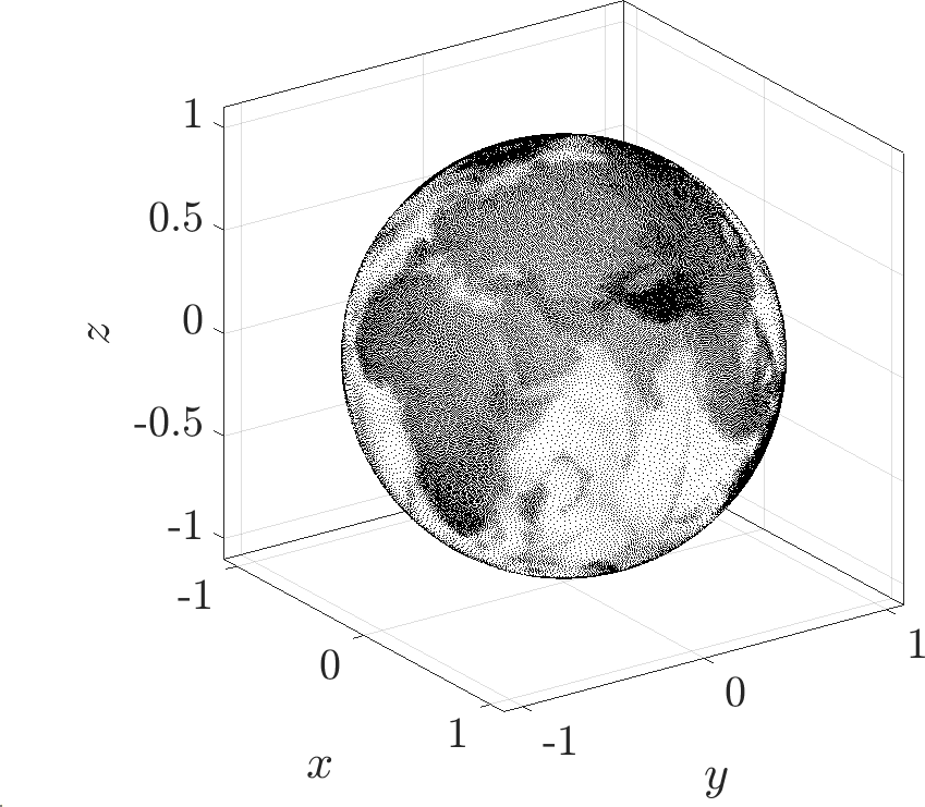
Figure 13: Spherical Earth model sampled proportionally with altitude, $N=100\,457$.

3.6 Computational complexity and execution time

Theoretical computational complexity of the proposed algorithm was already analyzed in Section 2.1, and was derived to be

(23) $$T_{\text{PA}}=O(nN\log N),$$

for the general version with a $k$-d tree spatial structure. The computational complexity of the naive algorithm is clearly

(24) $$T_{\text{NA}}=O(N),$$

since the parameters are generated on a grid inside a box-shaped parametric domain $\Xi$ and mapped to the surface.

The computational complexity of the supersampling-decimation algorithm can be written in terms of the number of generated parameters. If $N_{p}$ is the number of parameters that are generated in the parametric domain $\Xi$ with spacing $h_{\Xi}=h/\gamma$, the time complexity of the algorithm is $O(N_{p}\log(N_{p}))$, as the mapping of the parameters taken $O(N_{p})$ time and closest node queries take $\log(N_{p})$ per node using a $k$-d tree data structure. To compare this result other time complexities, it would need to be expressed in terms of $N$, the number of finally accepted nodes. It always holds that $N\leq N_{p}$, but relating $N$ to $N_{p}$ in the form of $N_{p}=O(f(N))$ is not trivial in general and depends on the parametrization $\boldsymbol{r}$. However, by our choice of $\gamma$ it can be estimated that the SD algorithm generates $\tau^{d_{\Xi}}|\operatorname{obb}\partial\Omega|/|\partial\Omega|$ more points than it returns, where $|\operatorname{obb}\partial\Omega|$ and $|\partial\Omega|$ are surface areas of the oriented bounding box and the parameterized surface, respectively. Thus we can informally estimate

(25) $$T_{\text{SD}}\approx O\left(\tau^{d_{\Xi}}\frac{|\operatorname{obb}\partial\Omega|}{|\partial\Omega|}N\log\left(\tau^{d_{\Xi}}\frac{|\operatorname{obb}\partial\Omega|}{|\partial\Omega|}N\right)\right).$$

To achieve good quality of nodes, the parameter $\tau$ needs to be as large or larger than $\max_{\boldsymbol{p}\in\partial\Omega}\|\nabla\boldsymbol{r}(\boldsymbol{p})\|$. Nonetheless, the supersampling-decimation algorithm can be faster than the proposed algorithm in many real world cases, while the proposed algorithm offers consistent execution time over a wider range of cases.

To compare the actual execution time of the three algorithms they were run with various $h$ on curve $\boldsymbol{r}_{p}$ (11) and the heart-like surface $\boldsymbol{r}_{h}$ (12). The measurements were done on a machine with an Intel(R) Xeon(R) CPU E5-2620 v3 @ 2.40GHz processor and 64 GB DDR3 RAM. Code was compiled with g++ (GCC) 8.1.0 for Linux with -std=c++11 -O3 -DNDEBUG flags. Measurements for each data point were executed 9 times and the median time was taken. The results are shown in Fig. 14.

Growth factors obtained from practical results match the theoretical time complexities. A different choice of $\tau$ can make the supersampling algorithm faster or slower than proposed algorithm. Both are able to generate $10^{6}$ nodes in order of a few seconds in $d_{\Xi}=1$ case and in order of few 10s of seconds in $d_{\Xi}=2$ case.

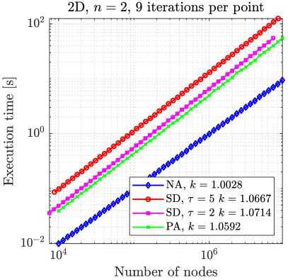
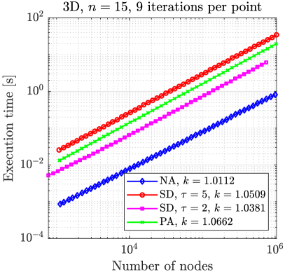
Figure 14: Execution time for different algorithms for different densities in 2D and 3D. Sampling of 2D polar curve from (11) and 3D heart-like surface from (12). The values $k$ represent the estimated line slopes.

4 Mesh-free numerical analysis example

In this section we demonstrate the performance of the proposed algorithm in providing the discretization of domain boundary for meshless solution of PDEs. Consider a domain $\Omega$ bounded by the polar curve $\boldsymbol{r}_{p}$ in 2D and bounded by the heart-like surface $\boldsymbol{r}_{h}$ in 3D.

For the closed form solution we choose $u_{2}(x,y)=\sin(\pi x)\cos(2\pi y)$ in 2D and $u_{3}(x,y,z)=\sin(\pi x)\cos(2\pi y)\sin(\frac{1}{2}\pi z)$ in 3D and define the following Poisson problem in $d$ dimensions (for $d=2,3$):

(26) $$\hskip 113.81102pt\nabla^{2}u =f \text{in $\Omega$},\hskip 113.81102pt$$

(27) $$\hskip 113.81102ptu =u_{d} \text{on $\Gamma_{e}$},\hskip 113.81102pt$$

(28) $$\hskip 113.81102pt\vec{n}\cdot\nabla u =g \text{on $\Gamma_{n}$},\hskip 113.81102pt$$

where $f$ and $g$ are computed from $u_{d}$.

The domain $\Omega$ is discretized in two steps. First, boundary $\partial\Omega$ is discretized using the proposed algorithm. In the second step, the interior of $\Omega$ is populated with nodes using the algorithm introduced in [25] where the boundary nodes from the first step are used as the seed nodes.

Once the domain is fully populated with nodes, a radial basis function-generated finite differences (RBF-FD) method, using polyharmonic basis functions augmented with monomials is used. RBF-FD using polyharmonics augmented with monomials is a promising mesh-free method that combines the robustness of classical RBF-FD but circumvents the stagnation errors and achieves high-order accuracy by leveraging monomial augmentation [1].

We used RBF-FD with monomial augmentation up to order $m\in\{2,4,6\}$, where we chose stencil size $n=4\binom{m+2}{2}$ in 2D and $n=4\binom{m+3}{3}$ in 3D, based on guidelines from [1], to obtain the mesh-free approximations of the differential operators involved. The resulting sparse system is solved with BiCGSTAB using an ILUT preconditioner.

Figures 15 and 16 show the relative discrete $p$-norm error $e_{p}=\|u-\hat{u}\|_{p}/\|u\|_{p}$ for increasing number of nodes in two cases. In one case, only Dirichlet boundary conditions were used ($\Gamma_{e}=\partial\Omega$ and $\Gamma_{n}=\emptyset$) and in the other case, labeled “mixed”, Dirichlet boundary conditions were used for boundary nodes with negative $x$-coordinate and Neumann boundary conditions were used otherwise.

The error behaves as expected in 3D, but starts diverging when the number of nodes is big in 2D. This is because of finite precision errors discussed by Flyer et al. [10]. Until that point, the error also behaves as expected in 2D.

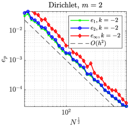
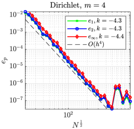
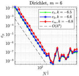
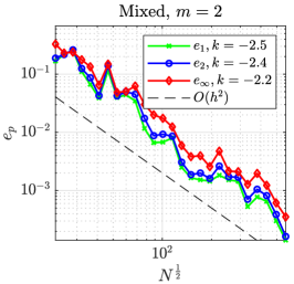
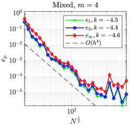
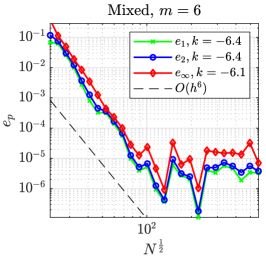
Figure 15: Convergence of Poisson’s equation $u(x,y)=\sin(\pi x)\cos(2\pi y)$ with different boundary conditions and monomials up to order $m$ on nodes generated by the proposed algorithm and the algorithm presented in [25] on 2D polar curve from (11). The values $k$ represent the estimated line slopes until the error starts diverging.

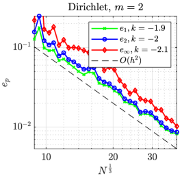
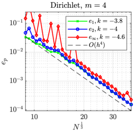
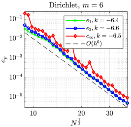
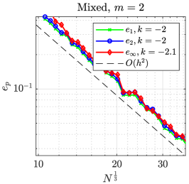
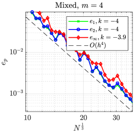
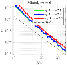
Figure 16: Convergence of Poisson’s equation $u(x,y,z)=\sin(\pi x)\cos(2\pi y)\sin(\frac{1}{2}\pi z)$ with mixed boundary conditions and monomials up to order $m$ on nodes generated by the proposed algorithm and the algorithm presented in [25] on 3D heart-like surface from (12). The values $k$ represent the estimated line slopes.

5 Conclusions

A new algorithm for generating nodes on parametric surfaces was developed and compared with naive parametric sampling and the supersampling-decimation algorithm [23]. All three algorithms require that a parametrization $\boldsymbol{r}$ of a curve/surface in question is given.

Of the three algorithms, both supersampling and the proposed algorithm produce quasi-uniform discretizations. The proposed algorithm requires that $\nabla\boldsymbol{r}$ is given in addition to $\boldsymbol{r}$, which can be problematic, but is usually known in case of closed form parametrization, RBF models or CAD models. Contrary to the other two algorithms, the proposed algorithm supports generation of nodes with variable nodal spacing, and on irregular parametric domains. It also adapts to parametrizations with variable $\|\nabla\boldsymbol{r}\|$ without modifications. We also proved minimal spacing requirements of the proposed algorithm, for both uniform and variable spacing.

Both the proposed and the supersampling-decimation algorithm support generation of nodes in arbitrary dimensions. The time complexity of the proposed algorithm is $O(N\log N)$ to generate $N$ nodes in all cases, while the time complexity of the supersampling algorithm varies a lot with $\tau$ and the properties of the parametrization $\boldsymbol{r}$. The execution times of the algorithm are comparable, with execution time of supersampling-decimation algorithm depending heavily on choice of $\tau$. It takes around 1 s to generate $10^{6}$ nodes in 2D and 10 s to generate $10^{6}$ nodes in 3D.

Future work is focused on the parallelization of the underlying spatial generation algorithm, with some successful preliminary results [6] and analyzing the behavior of the algorithm for surfaces composed of multiple patches, with the ultimate goal to support automatic meshless discretization of CAD models.

Appendix A Node spacing error proposition

Proposition 3.1.

The following estimates hold for the error of local node spacing radius due to linear approximation in (3):

(29) $$|\Delta h(\boldsymbol{\xi},\vec{s})| \leq\frac{\sqrt{d_{\Xi}}}{2}h(\boldsymbol{p})^{2}\frac{\displaystyle\max_{i=1,\ldots,d_{\Xi}}\max_{\theta\in[0,\alpha]}\left|\vec{s}^{\mathsf{T}}(\nabla\nabla r_{i})(\boldsymbol{\xi}+\theta\vec{s})\vec{s}\right|}{\|\nabla\boldsymbol{r}(\boldsymbol{\xi})\vec{s}\|^{2}},\alpha=\frac{h(\boldsymbol{p})}{\|\nabla\boldsymbol{r}(\boldsymbol{\xi})\vec{s}\|},$$

(30) $$|\Delta h(\boldsymbol{\xi})| \leq\frac{\sqrt{d_{\Xi}}}{2}h(\boldsymbol{p})^{2}\frac{\displaystyle\max_{i=1,\ldots,d_{\Xi}}\max_{\boldsymbol{\zeta}\in\bar{B}(\boldsymbol{\xi},\rho_{\boldsymbol{\xi}})}\sigma_{1}((\nabla\nabla r_{i})(\boldsymbol{\zeta}))}{\sigma_{d_{\Xi}}(\nabla\boldsymbol{r}(\boldsymbol{\xi}))^{2}},\;\rho_{\boldsymbol{\xi}}=\frac{h(\boldsymbol{p})}{\sigma_{d_{\Xi}}(\nabla\boldsymbol{r}(\boldsymbol{\xi}))},$$

(31) $$|\Delta h| \leq\frac{\sqrt{d_{\Xi}}}{2}h_{M}^{2}\frac{\sigma_{1,M}(\nabla\nabla\boldsymbol{r})}{\sigma_{d_{\Xi},m}^{2}(\nabla\boldsymbol{r})},$$

where

(32) $$h_{M} =\max_{\boldsymbol{\xi}\in\Xi}h(\boldsymbol{p}),$$

(33) $$\sigma_{1,M}(\nabla\nabla\boldsymbol{r}) =\max_{i=1,\ldots,d_{\Xi}}\max_{\boldsymbol{\xi}\in\Xi}\sigma_{1}((\nabla\nabla r_{i})(\boldsymbol{\xi})),$$

(34) $$\sigma_{d_{\Xi},m}(\nabla\boldsymbol{r}) =\min_{\boldsymbol{\xi}\in\Xi}\sigma_{d_{\Xi}}(\nabla\boldsymbol{r}(\boldsymbol{\xi})),$$

and $\sigma_{i}(A)$ denotes the $i$-th largest singular value of $A$.

In particular, this means that the relative error in spacing $|\Delta h|/h$ decreases linearly with $h$ for well behaved $\boldsymbol{r}$ and the algorithm for placing points on surfaces asymptotically retains the minimal spacing and quasi-uniformity bounds of the underlying algorithm for flat space.

Proof A.1.

The following estimate for $a\in\mathbb{R}$ and $b,c\in\mathbb{R}^{n}$ will be used:

(35) $$|a-\|b+c\||\leq|a-\|b\||+\|c\|.$$

The dependence of $\alpha$ on $\boldsymbol{\xi}$ and $\vec{s}$ will also be written explicitly, $\alpha(\boldsymbol{\xi},\vec{s})$. We begin to estimate the error locally

(36) $$|\Delta h(\boldsymbol{\xi},\vec{s})| \leq|h(\boldsymbol{p})-\hat{h}(\boldsymbol{\xi},\vec{s})|$$

(37) $$=|h(\boldsymbol{p})-\|\boldsymbol{r}(\boldsymbol{\eta})-\boldsymbol{r}(\boldsymbol{\xi})\||=|h(\boldsymbol{p})-\|\alpha(\boldsymbol{\xi},\vec{s})\nabla\boldsymbol{r}(\boldsymbol{\xi})\vec{s}+\boldsymbol{R}(\boldsymbol{\xi},\vec{s})\||$$

(38) $$\leq|h(\boldsymbol{p})-\|\alpha(\boldsymbol{\xi},\vec{s})\nabla\boldsymbol{r}(\boldsymbol{\xi})\vec{s}\||+\|\boldsymbol{R}(\boldsymbol{\xi},\vec{s})\|$$

(39) $$=\left|h(\boldsymbol{p})-\frac{h(\boldsymbol{p})}{\|\nabla\boldsymbol{r}(\boldsymbol{\xi})\vec{s}\|}\|\nabla\boldsymbol{r}(\boldsymbol{\xi})\vec{s}\|\right|+\|\boldsymbol{R}(\boldsymbol{\xi},\vec{s})\|$$

(40) $$=\|\boldsymbol{R}(\boldsymbol{\xi},\vec{s})\|,$$

where $\boldsymbol{R}(\boldsymbol{\xi},\vec{s})$ is the remainder of the Taylor approximation

(41) $$\boldsymbol{R}(\boldsymbol{\xi},\vec{s})=\boldsymbol{r}(\boldsymbol{\eta})-\boldsymbol{r}(\boldsymbol{\xi})-\alpha\nabla\boldsymbol{r}(\boldsymbol{\xi})\vec{s},$$

which can also we viewed as an Taylor expansion of $\boldsymbol{r}(\boldsymbol{p}+\alpha\vec{s})$ around $\alpha=0$. The remainder can be further estimated component-wise:

(42) $$\|\boldsymbol{R}(\boldsymbol{\xi},\vec{s})\|\leq\sqrt{d_{\Xi}}\max_{i=1,\ldots,d_{\Xi}}\|R_{i}(\boldsymbol{\xi},\vec{s})\|.$$

Using the Lagrange form of remainder for each component of $R(\boldsymbol{\xi})$, we arrive at

(43) $$R_{i}(\boldsymbol{\xi},\vec{s})=\frac{1}{2}h(\boldsymbol{p})^{2}\frac{\vec{s}^{\mathsf{T}}(\nabla\nabla r_{i})(\boldsymbol{\xi}+\theta\vec{s})\vec{s}}{\|\nabla\boldsymbol{r}(\boldsymbol{\xi})\vec{s}\|^{2}}$$

for some $\theta\in[0,\alpha]$, where $\nabla\nabla r_{i}$ is the Hessian matrix of $r_{i}$. Thus we can bound each component as

(44) $$|R_{i}(\boldsymbol{\xi},\vec{s})|\leq\frac{1}{2}h(\boldsymbol{p})^{2}\frac{\max_{\theta\in[0,\alpha]}|\vec{s}^{\mathsf{T}}(\nabla\nabla r_{i})(\boldsymbol{\xi}+\theta\vec{s})\vec{s}|}{\|\nabla\boldsymbol{r}(\boldsymbol{\xi})\vec{s}\|^{2}},$$

which gives us the local error bound for a point-candidate pair:

(45) $$|\Delta h(\boldsymbol{\xi},\vec{s})|\leq\frac{\sqrt{d_{\Xi}}}{2}h(\boldsymbol{p})^{2}\frac{\displaystyle\max_{i=1,\ldots,d_{\Xi}}\max_{\theta\in[0,\alpha]}\left|\vec{s}^{\mathsf{T}}(\nabla\nabla r_{i})(\boldsymbol{\xi}+\theta\vec{s})\vec{s}\right|}{\|\nabla\boldsymbol{r}(\boldsymbol{\xi})\vec{s}\|^{2}}.$$

To estimate the error around $\boldsymbol{p}$ for all candidates, we can further bound (44) more independently of $\vec{s}$ by using

(46) $$\|\nabla\boldsymbol{r}(\boldsymbol{\xi})\vec{s}\| \geq\sigma_{d_{\Xi}}(\nabla\boldsymbol{r}(\boldsymbol{\xi}))>0$$

(47) $$\left|\vec{s}^{\mathsf{T}}(\nabla\nabla r_{i})(\boldsymbol{\xi}+\theta\vec{s})\vec{s}\right| \leq\sigma_{1}((\nabla\nabla r_{i})(\boldsymbol{\xi}+\theta\vec{s}))$$

where $\sigma_{d_{\Xi}}$ is the smallest singular value of the Jacobian, which is positive as $\boldsymbol{r}$ is regular and $\sigma_{1}$ is the largest singular value of the Hessian. Following that, we can bound $R_{i}$ as

(48) $$|R_{i}(\boldsymbol{\xi},\vec{s})| \leq\frac{1}{2}h(\boldsymbol{p})^{2}\frac{\max_{\boldsymbol{\zeta}\in[0,\alpha]}\sigma_{1}((\nabla\nabla r_{i})(\boldsymbol{\xi}+\theta\vec{s}))}{\sigma_{d_{\Xi}}(\nabla\boldsymbol{r}(\boldsymbol{\xi}))^{2}}$$

(49) $$\leq\frac{1}{2}h(\boldsymbol{p})^{2}\frac{\displaystyle\max_{\boldsymbol{\zeta}\in\bar{B}(\boldsymbol{\xi},\rho_{\boldsymbol{\xi}})}\sigma_{1}((\nabla\nabla r_{i})(\boldsymbol{\zeta}))}{\sigma_{d_{\Xi}}(\nabla\boldsymbol{r}(\boldsymbol{\xi}))^{2}}$$

where

(50) $$\rho_{\boldsymbol{\xi}}=\frac{h(\boldsymbol{p})}{\sigma_{d_{\Xi}}(\nabla\boldsymbol{r}(\boldsymbol{\xi}))}\geq\alpha(\boldsymbol{\xi},\vec{s})$$

is the radius of the closed ball $\bar{B}(\boldsymbol{\xi},\rho_{\boldsymbol{\xi}})$ centered at $\boldsymbol{\xi}$. The inequality (49) holds as the maximum is sought over a larger domain. This gives the local estimate around a point as

(51) $$|\Delta h(\boldsymbol{\xi})|\leq\frac{\sqrt{d_{\Xi}}}{2}h(\boldsymbol{p})^{2}\frac{\displaystyle\max_{i=1,\ldots,d_{\Xi}}\max_{\boldsymbol{\zeta}\in\bar{B}(\boldsymbol{\xi},\rho_{\boldsymbol{\xi}})}\sigma_{1}((\nabla\nabla r_{i})(\boldsymbol{\zeta}))}{\sigma_{d_{\Xi}}(\nabla\boldsymbol{r}(\boldsymbol{\xi}))^{2}}.$$

To obtain a simple global estimate, we take the maximum of (51) over $\boldsymbol{\xi}$

(52) $$|\Delta h| \leq\max_{\boldsymbol{\xi}\in\Xi}\left(\frac{\sqrt{d_{\Xi}}}{2}h(\boldsymbol{p})^{2}\frac{\displaystyle\max_{i=1,\ldots,d_{\Xi}}\max_{\boldsymbol{\zeta}\in\bar{B}(\boldsymbol{\xi},\rho_{\boldsymbol{\xi}})}\sigma_{1}((\nabla\nabla r_{i})(\boldsymbol{\zeta}))}{\sigma_{d_{\Xi}}(\nabla\boldsymbol{r}(\boldsymbol{\xi}))^{2}}\right)$$

(53) $$\leq\frac{\sqrt{d_{\Xi}}}{2}h_{M}^{2}\frac{\displaystyle\max_{i=1,\ldots,d_{\Xi}}\max_{\boldsymbol{\xi}\in\Xi}\max_{\boldsymbol{\zeta}\in\bar{B}(\boldsymbol{\xi},\rho_{\boldsymbol{\xi}})}\sigma_{1}((\nabla\nabla r_{i})(\boldsymbol{\zeta}))}{\min_{\boldsymbol{\xi}\in\Xi}\sigma_{d_{\Xi}}^{2}(\nabla\boldsymbol{r}(\boldsymbol{\xi}))}$$

(54) $$\leq\frac{\sqrt{d_{\Xi}}}{2}h_{M}^{2}\frac{\sigma_{1,M}(\nabla\nabla\boldsymbol{r})}{\sigma_{d_{\Xi},m}^{2}(\nabla\boldsymbol{r})},$$

where

(55) $$h_{M} =\max_{\boldsymbol{\xi}\in\Xi}h(\boldsymbol{p}),$$

(56) $$\sigma_{1,M}(\nabla\nabla\boldsymbol{r}) =\max_{i=1,\ldots,d_{\Xi}}\max_{\boldsymbol{\xi}\in\Xi}\sigma_{1}((\nabla\nabla r_{i})(\boldsymbol{\xi})),$$

(57) $$\sigma_{d_{\Xi},m}(\nabla\boldsymbol{r}) =\min_{\boldsymbol{\xi}\in\Xi}\sigma_{d_{\Xi}}(\nabla\boldsymbol{r}(\boldsymbol{\xi})),$$

and the equality in (56) holds since the inner maximum over local balls is superfluous when the maximum is sought over the whole domain. In particular, if $h$ is constant, the absolute error is of order $h^{2}$ and the relative error is linear.

References

- [1] V. Bayona, N. Flyer, B. Fornberg, and G. A. Barnett, On the role of polynomials in RBF-FD approximations: II. Numerical solution of elliptic PDEs, J. Comput. Phys., 332 (2017), pp. 257–273, https://doi.org/10.1016/j.jcp.2016.12.008.
- [2] J. L. Blanco and P. K. Rai, nanoflann: a C++ header-only fork of FLANN, a library for nearest neighbor (NN) with KD-trees, 2014, https://github.com/jlblancoc/nanoflann.
- [3] R. Bridson, Fast Poisson disk sampling in arbitrary dimensions, in SIGGRAPH sketches, 2007, p. 22, https://doi.org/10.1145/1278780.1278807.
- [4] J. C. Carr, R. K. Beatson, B. C. McCallum, W. R. Fright, T. J. McLennan, and T. J. Mitchell, Smooth surface reconstruction from noisy range data, in Proceedings of the 1st international conference on Computer graphics and interactive techniques in Australasia and South East Asia, ACM, 2003, pp. 119–ff.
- [5] Data announcement 88-MGG-02, Digital relief of the surface of the Earth. NOAA, National Geophysical Data Center, Boulder, Colorado, 1988, https://www.ngdc.noaa.gov/mgg/global/etopo5.html.
- [6] M. Depolli, G. Kosec, and J. Slak, Parallelizing a node positioning algorithm for meshless methods, in ParNum 2019 book of abstracts, 13th Parallel numerics workshop, Dubrovnik, Croatia,, University of Zagreb, 2019, https://www.fsb.unizg.hr/parnum2019/abs_book_web.pdf.
- [7] P. Diaconis, S. Holmes, M. Shahshahani, et al., Sampling from a manifold, in Advances in modern statistical theory and applications: a Festschrift in honor of Morris L. Eaton, Institute of Mathematical Statistics, 2013, pp. 102–125.
- [8] U. Duh, G. Kosec, and J. Slak, Standalone implementation of the proposed algorithm. http://e6.ijs.si/medusa/static/PA.zip.
- [9] N. Flyer, G. A. Barnett, and L. J. Wicker, Enhancing finite differences with radial basis functions: Experiments on the navier–stokes equations, Journal of Computational Physics, 316 (2016), pp. 39 – 62, https://doi.org/10.1016/j.jcp.2016.02.078.
- [10] N. Flyer, B. Fornberg, V. Bayona, and G. A. Barnett, On the role of polynomials in RBF-FD approximations: I. Interpolation and accuracy, Journal of Computational Physics, 321 (2016), pp. 21–38, https://doi.org/10.1016/j.jcp.2016.05.026.
- [11] B. Fornberg and N. Flyer, Fast generation of 2-D node distributions for mesh-free PDE discretizations, Computers & Mathematics with Applications, 69 (2015), p. 531–544, https://doi.org/10.1016/j.camwa.2015.01.009.
- [12] X. D. Gu, W. Zeng, F. Luo, and S.-T. Yau, Numerical computation of surface conformal mappings, Computational Methods and Function Theory, 11 (2012), pp. 747–787, https://doi.org/10.1007/BF03321885.
- [13] G. Guennebaud, B. Jacob, et al., Eigen v3, 2010, http://eigen.tuxfamily.org.
- [14] D. P. Hardin, T. Michaels, and E. B. Saff, A comparison of popular point configurations on , Dolomites Research Notes on Approximation, 9 (2016).
- [15] D. P. Hardin and E. B. Saff, Discretizing manifolds via minimum energy points, Notices of the AMS, 51 (2004), pp. 1186–1194.
- [16] N. P. Kopytov and E. A. Mityushov, Uniform distribution of points on hypersurfaces: simulation of random equiprobable rotations, Vestnik Udmurtskogo Universiteta. Matematika. Mekhanika. Komp'yuternye Nauki, 25 (2015), pp. 29–35, https://doi.org/10.20537/vm150104.
- [17] G. Kosec, A local numerical solution of a fluid-flow problem on an irregular domain, Adv. Eng. Software, 120 (2018), pp. 36–44, https://doi.org/10.1016/j.advengsoft.2016.05.010.
- [18] T. S. Lau, S. H. Lo, and C. K. Lee, Generation of quadrilateral mesh over analytical curved surfaces, Finite Elements in Analysis and Design, 27 (1997), pp. 251–272, https://doi.org/10.1016/S0168-874X(97)00015-2.
- [19] N. Litke, A. Levin, and P. Schröder, Fitting subdivision surfaces, in Proceedings of the conference on Visualization’01, IEEE Computer Society, 2001, pp. 319–324.
- [20] Medusa library, http://e6.ijs.si/medusa/.
- [21] A. W. Moore, An introductory tutorial on kd-trees, phdthesis 209, Computer Laboratory, University of Cambridge, 1991, https://www.ri.cmu.edu/pub_files/pub1/moore_andrew_1991_1/moore_andrew_1991_1.pdf.
- [22] L. Piegl and W. Tiller, The NURBS book, Springer Science & Business Media, 2012.
- [23] V. Shankar, R. M. Kirby, and A. L. Fogelson, Robust node generation for meshfree discretizations on irregular domains and surfaces, SIAM J. Sci. Comput., 40 (2018), pp. 2584–2608, https://doi.org/10.1137/17m114090x.
- [24] K. Shimada and D. C. Gossard, Automatic triangular mesh generation of trimmed parametric surfaces for finite element analysis, Computer Aided Geometric Design, 15 (1998), pp. 199–222, https://doi.org/10.1016/s0167-8396(97)00037-x.
- [25] J. Slak and G. Kosec, On generation of node distributions for meshless PDE discretizations, SIAM Journal on Scientific Computing, 41 (2019), pp. A3202–A3229, https://doi.org/10.1137/18M1231456.
- [26] I. Stroud, Boundary representation modelling techniques, Springer Science & Business Media, 2006.
- [27] G. Turk, Texture synthesis on surfaces, in Proceedings of the 28th annual conference on Computer graphics and interactive techniques, ACM, 2001, pp. 347–354, https://doi.org/10.1145/383259.383297.
- [28] O. Vlasiuk, T. Michaels, N. Flyer, and B. Fornberg, Fast high-dimensional node generation with variable density, Computers & Mathematics with Applications, 76 (2018), pp. 1739 – 1757, https://doi.org/10.1016/j.camwa.2018.07.026.
- [29] H. Wendland, Scattered data approximation, vol. 17, Cambridge university press, 2004.
- [30] R. Zamolo and E. Nobile, Two algorithms for fast 2d node generation: Application to rbf meshless discretization of diffusion problems and image halftoning, Computers & Mathematics with Applications, 75 (2018), pp. 4305–4321, https://doi.org/10.1016/j.camwa.2018.03.031.
- [31] H.-K. Zhao, S. Osher, and R. Fedkiw, Fast surface reconstruction using the level set method, in Proceedings IEEE Workshop on Variational and Level Set Methods in Computer Vision, IEEE, 2001, pp. 194–201.