Toward ultrametric modeling of the epidemic spread
Abstract
An ultrametric model of epidemic spread of infections based on the classical SIR model is proposed. Ultrametrics on a set of individuals is introduced based on their hierarchical clustering relative to the average time of infection contact. The general equations of the ultrametric SIR model are written down and their particular implementation using the -adic parametrization is presented. A numerical analysis of the -adic SIR model and a comparison of its behavior with the classical SIR model are performed. The concept of hierarchical isolation and the scenario of its management in order to reduce the level of epidemic spread is considered.
Keywords: SIR model, hierarchical clustering, ultrametrics, -adic models, epidemic spread.
1 Introduction
Recently, there has been activity in the development of mathematical models of the spread of infectious diseases (see, for example, [1, 2, 3, 4, 5]). This is primarily due to both the detection of old foci of existing viral infections, such as plague, anthrax, Ebola, and the emergence of the new infections caused by coronaviruses such as SARS-CoV (2002), MERS-CoV (2015), and SARS-CoV-2 (2019). Almost all mathematical models describing the development of epidemics are based on the model proposed in 1927 by Kermack and McKendrick in work [6], which is now known as the classic SIR model. This model is based on 3-step development of the epidemic, in which healthy but susceptible individuals (S) as a result of infection go to the infected class (I) individuals who, in turn, move to the removed class (R), i.e. recover by acquiring immunity, or die. Note that the SIR model was constructed by analogy with the theory of homogeneous chemical reactions. This model has many generalizations that include additional intermediate stages of individuals known as SIRS, SEIR, SEIRS, and others.
The essence of the simplest SIR model is as follows. Let is the number of susceptible, is the number of infected, is the number of removed individuals. The following simplifying assumptions are accepted: 1) the set of individuals is homogeneous; 2) the number of individuals under consideration (susceptible, infected and removed) is constant, i.e. ; 3) the probability of transmission per unit time from an infected individual to a susceptible individuals is constant; 3) the probability of reinfection is zero. Given these simplifying assumptions the SIR model equations are written as
| (1) |
| (2) |
| (3) |
Here is infection rate (or the average number of contacts with susceptible individuals that leads to the new infected individuals per time unit per infective), and is removing rates (or the average rate of removal of infective per unit time per infective).
| (4) |
where and is reproductive ratio. It follows from (4) that
| (5) |
where . Equation (5) with is solvable for on the segment only under condition and there is no solutions on this segment when . For this reason, condition is interpreted in this model as an outbreak condition of epidemic. Today, many generalizations of the classic SIR model have been proposed, which use more complex scenarios for the development of the epidemic, taking into account the latency period, the finiteness of the time when individuals are in the stage of immunity, the impact of vaccination, etc. The classical SIR model, as well as most of its generalizations, are essentially homogeneous models, i.e. they assume that the intensity of infection does not depend on any relationship between susceptible and infected individuals. Nevertheless, even in such homogeneous models, adequate estimates of the scenario for the development of real epidemics are possible. Recently, a number of heterogeneous generalizations of the SIR models based on deterministic or random networks have also been proposed (see, for example, [7, 8, 9, 10]), taking into account the heterogeneous nature of the populations in which the epidemic is spreading. As a rule, this heterogeneity is associated with the difference in the characteristics of individuals, or with the heterogeneity of population density.
Meanwhile, the most important characteristic that plays a crucial role in the speed of spread of the epidemic is the distribution of the time duration of infectious contact between pairs of individuals. This value can be a characteristic of population heterogeneity, and it allows us to introduce a distance function on a set of individuals (metric) in terms of which it is possible to generalize the classical SIR model.
In this paper, we propose an inhomogeneous generalization of the classical SIR model, which is based on the hierarchical clustering of the population according to the degree of potential infectious influence of individuals on each other. We describe the procedure for such hierarchical clustering of a set of individuals and show that such clustering involves the introduction of a distance function on the set of individuals, which is ultrametrics. This distance function is not directly related to the spatial distance between individuals, it is determined only by the potential for transmission of infection from one individual to another per unit time. Using the ultrametric distance on a set of individuals, we generalize the equations of the classical SIR model and arrive at a model that we call the basic ultrametric SIR model. As known, a convenient tool for parameterizing ultrametric spaces is the field of -adic numbers. We consider the ultrametric set of individuals that can be maped to the boundary of a finite hierarchical graph with a constant number of branches. Such a set can be parameterized by the set of a -adic balls of unit radius contained in a -adic ball of radius greater than 1. We call the corresponding ultrametric SIR model the -adic SIR model. We present a numerical analysis of the -adic SIR model and compare its behavior with the classical SIR model. We also introduce the concept of hierarchical isolation index and consider the simplest scenario for managing this parameter in order to reduce the spread of the epidemic.
2 Hierarchical clustering of human population and ultrametric
Let be a set of individuals. Infectious contact of two individuals and we will call any continuous time interval which satisfies the condition: during interval one of the individuals (for example, ) can be infected by another individual , provided that individual is infected throughout the entire interval , and the probability of infection per unit time is non zero on interval on almost everywhere.
Note that the concept of an infectious contact is a purely model. In almost every specific case, the value of the infective contact is extremely difficult to calculate accurately, but it is always possible to approximate it. However, in any real assessment of the duration of an infectious contact, it must be understood that this concept does not necessarily mean physical contact between two individuals. The probability of infection of one individual by another individual may occur indirectly, i.e. through a physical contact with surrounding bodies (air, objects) that became sources of infection after a physical contact with an infected individual. However, an infectious contact does not imply the possibility of infection of a susceptible individual by an already infected individual through any other individuals. Intuitively speaking, the term “infectious contact” is a continuous period of time during which a particular individual has the potential for infection (no matter how small it is) at any time, and this possibility of infection is caused by a particular other individual.
Let be the value of a certain time interval during which we observe the behavior of individuals. Then for individual , there is a finite number of infectious contacts , with individual during this interval. Denote by the sum of the interval lengths . Obviously always . Since the behavior of individuals is random, is a random function which depends on the specific implementation of an ensemble of populations of individuals. Expected value is the average time of an infectious contact between two individuals during interval . It is obvious that the function is symmetric.
Function plays the main role in the hierarchical clustering of individuals, which we describe below. Consider an infinite decreasing sequence of numbers of real positive numbers , such that . Let’s divide all the set of individuals into groups , , …, , as follows. We will require that for any and for any individual there exists another individual from the same group for which inequality holds. Obviously, this partition is the only one. It then follows that if , then and then we have . Groups will be called the first level clusters.
First level clusters can be combined into larger sets of individuals – the second level clusters, which we will denote by , , …, , , . In this case, we require that for any individual there exists another individual from the same cluster for which inequality holds. It is obvious that if , then and then . Also for any if and we have if and belong to the same first level cluster and if and belong to different first level clusters. Similarly the clusters of the second level can be combined into third level clusters , , …, , , . For any individual , there exists another individual from the same cluster for which inequality holds. The third level clusters can be combined into fourth level clusters , , …, , , , and so on. This procedure of hierarchical clustering of individuals must eventually be interrupted, because at some -th step we will get a single cluster of -th level that will coincide with the set of individuals . For any individual , there exists an individual for whisch holds.
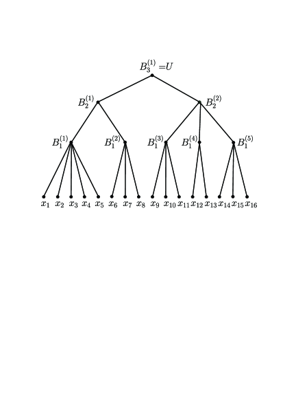
So, the hierarchical procedure for clustering individuals described above allows us to introduce on set the structure of hierarchically nested clusters . By construction, any two clusters of arbitrary levels either do not intersect, or one is contained in the other. The resulting hierarchical structure of clusters at various levels can be described by a hierarchical graph. An example of such a graph is shown in Figure 1.
Hierarchical clustering of the set of individuals allows us to introduce the ultrametrics on this set. We define function in the following way. If individuals and belong to the same level cluster, but belong to different level subclusters, then we put . If , we will put .
Proposition. Function is ultrametric, i.e. it satisfies the strong triangle inequality
| (6) |
Proof. To prove that function is ultrametric, it is sufficient to prove that any “triangle” , where , , is isosceles, and the two largest “sides” are equal. Let . Then by definition , individuals and belong to some level cluster , but they belong to different subclusters and level . Next, we have , . Suppose that inequalities and hold. Then each of the pairs and belongs to some cluster of a level smaller than . Let , , where . Both clusters and contain the same element . Therefore, one of them is contained in the other. Then the larger cluster must contain all three individuals . But this means that and are contained in a cluster of a level smaller than . Therefore, inequalities and cannot simultaneously be satisfied. Hence either , or . The proposition is proven.
3 Ultrametric formulation of the SIR model
In its meaning, ultrametrics on a set of individuals is a value equal to the ratio of the population observation time to the minimum boundary value of the average times of infectious contact of any two individuals belonging to the same minimal cluster as individuals and . We make the model assumption that the probability of infection of a susceptible individual by an infected individual per unit time is proportional to value . Naturally, this assumption is rather a rough approximation, since it assumes that during the infectious contact of individuals, the probability of infection per unit time of a susceptible individual infected is constant. Naturally, real function is not constant and depends on many factors (contact space, pathogen concentration, individual susceptibility, etc.). However, this approximation allows us to simplify the model significantly, while preserving its main quality property – the hierarchical nature of the development of the epidemic.
Let , , be the probability that at time , individual is correspondingly susceptible, infected, or removed. Then we can write the following ultrametric generalization of the equations (1) – (3)
| (7) |
| (8) |
| (9) |
Function
| (10) |
makes sense of the probability of infection by an infected individual of a susceptible individual per unit time. For large , the total number of susceptible, infected, and removed individuals is
| (11) |
Then in the case of the triviality of ultrametrics
and the independence of the functions , , from variable , taking into account , , , we get the system of equations
4 -adic parametrization of the ultrametric SIR model
Recall the definition of -adic number. Let be a field of rational numbers and let be a fixed prime number. Any rational number is uniquely represented as
| (12) |
where is an integer, and , are natural numbers that are not divisible by and have no common multipliers. The -Adic norm of number is defined by the equalities , . The field of -adic numbers is defined as a completion of the field of rational numbers by -adic norm . The norm on induces the metric which is ultrametric, i.e. satisfies the strong triangle inequality (6). We will denote: – a ball of radius centered at point , – a sphere of radius centered at point , , , . On there exists a unique (up to a factor) Haar measure which is invariant with respect to translations . We assume that is a full measure; that is,
| (13) |
Under this hypothesis the measure is unique. For more information about -adic numbers, the -adic analysis and its applications, see [11, 12, 13].
For our purposes, we can assume that number is a natural number . In this case is a ring of -adic numbers with the pseudo-norm , which also induces on the ultrametrics [14]. So let be a natural number. Further, let each level cluster contains exactly level clusters, the number of levels is , and the total number of individuals is . In this case, the set of individuals can be parameterized by the factor set and we assume that . Alternatively, we can describe the set of individuals by , but assume that each individual is described by a ball of unit radius.
Let be an arbitrary non-negative non-decreasing function defined on and satisfy the condition . Then function is also an ultrametrics on and we can write the equations of the basic ultrametric SIR model (7) – (9) in the form:
| (14) |
| (15) |
| (16) |
where
| (17) |
To preserve the interpretation, we will assume that functions , , lie in the class . Here is the class of functions that are constant on any ball of unit radius, is the class of functions that are integrable on and is the class of functions that are differentiable with respect to .
As each individual is described by a ball of unit radius. In this case, the possible non-zero values of ultrametrics (17) are , . This means that the ratio of boundaries of an average infection contact times of individuals belonging to different maximum subclusters of level and clusters is
| (18) |
In the -adic model under consideration, we will call value the hierarchical isolation index.
We will assume that coefficient depends on . We fix this dependence by requiring that the average value of of function (10) over all pairs of individuals, coincides with , where is an infection rate of classic SIR model. In this case we have
Imposing the requirement we get
and . Thus, the -adic SIR model is characterized by the following parameters: is the number of maximum subclusters for each cluster; is the number of levels for hierarchical clustering; is an infection rate of classical SIR model; is an removing rate; , where is the ratio of the boundaries of the average times of an infectious contact of individuals belonging to different maximum subclusters of clusters of neighboring levels.
5 Numerical analysis of the -adic SIR model and management of hierarchical isolation
Let there be a single infected individual at the initial time . This means the following choice of initial conditions of the Cauchy problem for equations (14) – (16):
where
From the structure of equations (14) – (16) and the type of function (17), it follows that functions , , will be constant on subsets for . We denote by a characteristic function of a subset of . Then functions , , can be decomposed by the basis of functions :
| (19) |
| (20) |
| (21) |
The total number of susceptible, infected, and removed individuals is
| (22) |
| (23) |
| (24) |
Below we investigate numerical solutions of equation (19) – (21) by Runge-Kutta-Fehlberg 45 method. Figure 2 shows the dependence of the cumulative number of infected individuals on time in the classical and -adic SIR models.
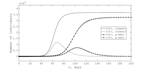
In doing so, we have chosen (the number of individuals in the minimal cluster), (the number of clusters), and . The value of an infection rate for the classical SIR model is chosen as . We also choose the average time of the disease course is equal 10 days, which corresponds to value . Accordingly, the reproductive ratio for the classical SIR model is (for comparison, the reproductive ratio for flu is , for COVID-19 [15]). For these parameters, we have 2.24 and the ratio of the maximum and minimum average time of an infection contact between individuals is . The initial conditions of the Cauchy problem of equations (19) - (21) are chosen as , . This corresponds to one infected individual at the initial time.
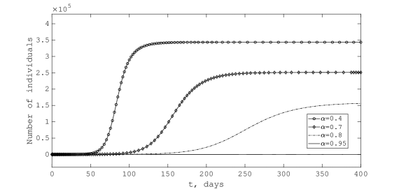
Figure 3 and Figure 4 show similar dependencies for values and , respectively, and unchanged other parameters The values of and respectively are =3.62 , for Figure 3 and , for Figure 4. Figure 4 corresponds to the case of a very weak spread of the epidemic in the -adic model.
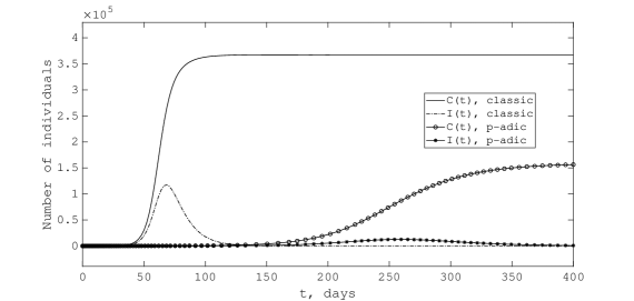
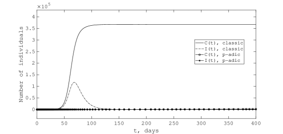
Fig. 5 shows dependence of the cumulative number of infected individuals in -adic SIR model for parameters , , , and different . As it can be seen from these dependencies there must exist critical such that at the spread of the epidemic takes place, but at the epidemic does not spread. For values ,, , , we have the numerical value of . Unfortunately, we could not get an exact analytical expression for function .
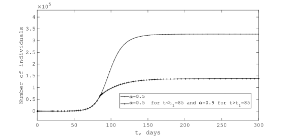
In the -adic SIR model, the hierarchical isolation index (18) can be considered as a control parameter that can be changed to control the spread of an epidemic. To illustrate, we will consider a situation where, as the epidemic grows, enforcement restrictions are introduced to redistribute the time of an infectious contact between individuals in clusters of different levels, while maintaining the average contact time is constant. In reality, the introduction of such restrictions means that an infectious contact between pairs of individuals with a small ultrametric distance must be increased, and an infectious contact between pairs of individuals with a large ultrametric distance must be decreased. In the -adic model, the introduction or strengthening of already introduced restrictions means an increase in the parameter. In Figure 6, we present dependence of the cumulative number of infected individuals in the case of controlling their hierarchical isolation, i.e., increasing the value of parameter at time from value to value with other parameters equal to , , , . We see that taking an adequate enforcement restriction to increase the hierarchical isolation index from to reduces the cumulative number of infected by more than 2 times.
6 Conclusion
In this paper, we have developed an ultrametric model of the epidemic spread of infection in the population, based on the classical SIR model. This model is also based on the concept of an infectious contact between any two individuals in the population, which determines the potential for transmission of infection from one individual to another. The formalization of this concept leads to hierarchical clustering of the population and the introduction of the ultrametric distance on a set of individuals. The ultrametric distance between individuals reflects the measure of transmission of infection between individuals and is included in the ultrametric generalization equations of the classical SIR model.
Changing the ultrametric structure of the proposed model can affect the spread of the epidemic in the population. Therefore, in contrast to the classic SIR model and its modifications, the proposed model can provide recommendations for avoiding a cumulative scenario of epidemic development based on managing the process of an infectious interaction between clusters of individuals at various levels. This corresponds to a certain algorithm for isolating separate social strata of the population at the micro, meso, and macro levels.
In conclusion, we note that the ultrametric model proposed in this paper is the basic model. It can be supplemented with various additional scenarios, such as the possibility of re-infection, the latent period, the time spent by individuals in the immune stage, the impact of vaccination, etc. We reserve the implementation and application of numerous extensions of the basic ultrametric model for future research.
The study was supported in part by the Ministry of Education and Science of Russia by State assignment to educational and research institutions under project FSSS-2020-0014.
References
- [1] R. Anderson and R. May, Infection Deseases of Humans: Dynamics and Control, New York, Oxford University Press, 1992.
- [2] O. Diekmann and J.A.P. Heesterbeek, Mathematical Epidemiology of Infectious Diseases: Model Building, Analysis and Interpretation, John Wiley and Sons, 2000.
- [3] M. Keeling and P. Rohani, Modeling Infectious Diseases in Humans and Animals, Princeton University Press, 2007.
- [4] F. Brauer F and C. Castillo-Chavez, Mathematical models in population biology and epidemiology. Springer, 2012.
- [5] Z. Wang, C.T. Bauch C.T., S. Bhattacharyya, et al., Statistical physics of vaccination, Phys. Rep., 664, 2016, 1–113.
- [6] W.O. Kermack and A.G. McKendrick, Contribution to the Mathematical Theory of Epidemics, Proceedings of the Royal Statistical Society A, 115, 1927, 700–721.
- [7] A.L. Lloyd and R.M. May, How viruses spread among computers and people, Science, 2001292 (5520), 2001, 1316–1317.
- [8] Y. Moreno, R. Pastor-Satorras and A. Vespignani, Epidemic outbreaks in complex heterogeneous networks. The European Physical Journal B-Condensed Matter and Complex Systems, 26 (4), 2002, 521–529.
- [9] R. Yang, B.H. Wang, J. Ren, W.J. Bai, Z.W. Shi, W.X. Wang, and T. Zhou, Epidemic spreading on heterogeneous networks with identical infectivity, Physics Letters A, 364 (3-4), 2007, 189–193.
- [10] E. Volz, SIR dynamics in random networks with heterogeneous connectivity. Journal of mathematical biology, 56 (3), 2008, 293–310.
- [11] B. Dragovich, A. Yu. Khrennikov, S. V. Kozyrev and I. V. Volovich, On -adic mathematical physics, -Adic Numbers, Ultrametric Analysis and Applications 1 (1), 2009, 1–17.
- [12] V. S. Vladimirov, I. V. Volovich and E. I. Zelenov, -Adic analysis and mathematical physics, World Sci. Publishing, Singapore, 1994.
- [13] W.H. Schikhof, Ultrametric calculus. An Introduction to -adic Analysis, Cambridge Studies in Advanced Mathematics, Cambridge University Press, Cambridge, 1984.
- [14] M.V. Dolgopolov, and A.P. Zubarev, Some aspects of the -adic analysis and its applications to -adic stochastic processes, -Adic Numbers, Ultrametric Analysis and Applications 3 (1), 2009, 39–51.
- [15] S. Sanche, Y.T. Lin, C. Xu, E. Romero-Severson, N. Hengartner and R. Ke, High Contagiousness and Rapid Spread of Severe Acute Respiratory Syndrome Coronavirus 2, Emerging infectious diseases, 26 (7), 2020.