Space-time metamorphosis

Abstract

We study the problem of registering images. The framework we use is metamorphosis and we construct a variational Eulerian space-time setting and pose the registration problem as an infinite-dimensional optimisation problem. The geodesic equations correspond to a system of advection and continuity equations and are solved analytically. Well-posedness of a primal conforming finite element method is established and its convergence is investigated numerically. This provides a discrete forward operator for the matching parameterized by a space-time velocity field. We propose a gradient descent method on this control variable and show several promising numerical results for this approach. Shape analysis; Metamorphosis; Finite element method.

1 Introduction

In shape analysis, metamorphosis [51, 30] is a metric framework for shape matching between potentially topologically different shapes. This image registration framework is a special case of Grenander’s group action model using the theory of deformable templates [24, 26]. In this setting, registration (or matchings) between different shapes (or deformable templates) are found by identifying the action in some group of transformations so that the application of the group action maps between the two shapes. A particular strength of the group action framework is its ability to handle the non-linear nature of shapes. Equipping a shape space with a metric not only provides a quantitative measure of closeness but also generates a meaningful way of interpolating, in sense of the prescribed metric, between elements of the space. In this paper, shapes are images given as functions with compact support on some polygonal Lipschitz domain where the goal is to match a template image $I_{0}$ with a target $I_{1}$ using metamorphosis. We aim to solve the geodesic equations associated with the energy of the matching in a space-time Eulerian frame and discretize these partial differential equations (PDEs) using the finite element method. Defining solution spaces over space-time allows us to leverage computational platforms featuring parallelism in both space and time at the expense of dealing with a larger system. This then defines a forward operator taking as input a time-dependent family of velocity fields and provides the associated geodesics for the images, motivating a gradient descent method to solve the inverse problem for the space-time velocity. Applications are manifold in everything from medical imaging to music videos [37, 6, 5, 52, 19, 23, 7, 3].

Diffeomorphic matching frameworks such as the popular large deformation diffeomorphic metric mapping (LDDMM) approach [6] preserve the underlying topology of the shapes on which they act. This class of methods relies on an observation in [2] that spaces of smooth vector fields $V$ generate a subgroup of diffeomorphisms ${\textnormal{Diff}_{V}}$ of some shape space via the following ODE:

$$\dot{\varphi}_{t}=u_{t}\circ\varphi_{t},\qquad t\in[0,1],$$

where $u_{t}\in V$, $\varphi_{t}\in{\textnormal{Diff}_{V}}$ and $\dot{g}=\frac{\partial g}{\partial t}$. A match between two shapes $I_{0}$ and $I_{1}$ is therefore given by the curve of diffeomorphisms that minimize the quantity:

$$\int_{0}^{1}\|u_{t}\|_{V}^{2}\,\textnormal{d}{t}+c\|I_{1}-I_{0}\circ\varphi_{1}^{-1}\|^{2},$$

for some penalty parameter $c>0$ where the first term is referred to as the kinetic energy. This approach was, to the best of the authors’ knowledge, first used for matching problems in [15, 48] with further early applications in [49]. $\|\cdot\|_{V}$ is typically some higher-order Sobolev norm or induced by a smooth kernel. See also [54] for a textbook on shapes and diffeomorphisms and [4, 13] for an overview of the diffeomorphism group and Riemannian geometry for shape analysis. When a purely diffeomorphic matching is no longer possible or necessary, metamorphosis allows for shape matching with topological changes. An early example of this is in [25] where the growth represents a tumour appearing on a medical image over the course of time. For the technical development of metamorphosis we refer to [40, 39]. [50] takes a more geometric point of view and describes in great detail a Riemannian construction.

First, we introduce some basic notation in order to sketch the main ideas of this paper and our contribution to the literature. ${\omega}=[0,1]^{d}$ denotes the spatial $d$-dimensional unit domain representing the spatial dimension of the images we are matching and we let $\Omega=[0,1]\times{\omega}$, where the first coordinate denotes time. ${\omega}$ will in certain cases be periodic in its $d$ dimensions. We let $\Gamma_{0}$ and $\Gamma_{1}$ denote the $d$-dimensional submanifolds of $\Omega$ given by the restriction of $\Omega$ in the first coordinate to the boundaries i.e. $t=0$ and $t=1$ specifying where we impose the images $I_{j}$, $j=0,1$ that we aim to match. When $d=1$, $\Omega$ is a simple unit square and $\Gamma_{j}$, $j=1,0$ are simply opposite boundaries; for $d=2$ these are opposing facets of the unit cube. Further we let $\Gamma=\Gamma_{0}\cup\Gamma_{1}$. Similarly, we shall sometimes use the notation $\Omega_{t}={\omega}$, $t\in[0,1]$. For ease of notation we define the operator $\frac{\partial}{\partial t}+u\cdot\nabla\equiv\mathbf{b}\cdot\nabla_{t}$ taking values in a real Hilbert space $G$ that we define later on. Here we use the $d$-dimensional row vector $\mathbf{b}=(u,\,1)^{\top}$, $\nabla_{t}=(\nabla,\frac{\partial}{\partial t})$ and $-\,\textnormal{div}_{t}$ its adjoint. In the following $\|\cdot\|_{0,\Omega}$ is the $L^{2}(\Omega)$ norm, and note that this is over space-time. Furthermore, let ${L^{2}([0,1],V)}$ denote functions $v$ such that for $t\in[0,1]$, $t\mapsto\|v(\cdot,t)\|_{V}$ is $L^{2}$ and for $x\in\omega$, $x\mapsto v(x,t)$ is in $V$. We can compute a metamorphic matching between $I_{0}$ and $I_{1}$ be solving the following infinite-dimensional optimisation problem:

$$\inf_{u\in{L^{2}([0,1],V)},I\in G}\quad \frac{1}{2}\int_{0}^{1}\frac{1}{2}\|u\|_{V}^{2}\;\textnormal{d}t+\sigma^{-2}\|\mathbf{b}\cdot\nabla_{t}I\|_{0,\Omega}^{2}$$ (1a)

subject to $$I|_{\Gamma_{j}}=I_{j},\quad j=0,1,$$ (1b)

where $u$ and $I$ depend both on space and time and $\sigma^{-2}>0$ is a penalty parameter. (1b) is understood in an $L^{2}(\Omega)$ sense. We aim to solve a type of relaxation of (1) and implicitly define $I$ by the velocity via a forward operator in the form of a PDE. Indeed for fixed $u$, the second term in (1) is a least-squares advection problem for $I$. With the previous idea in mind we write (1) as:

$$\inf_{(u,z)\in{L^{2}([0,1],V)}\times{L^{2}(\Omega)}}\quad \frac{1}{2}\int_{0}^{1}\|u\|_{V}^{2}\;\textnormal{d}t+\sigma^{-2}\|z\|_{0,\Omega}^{2}$$ (2a)

subject to $$z=\mathbf{b}\cdot\nabla_{t}I^{*}[u]\quad\textnormal{in } L^{2}(\Omega)$$ (2b)

$$I^{*}[u]\triangleq\arg\inf_{\begin{subarray}{c}I\in G,\\ I|_{\Gamma_{0}}=I_{0},\\ I|_{\Gamma_{1}}=I_{1}\end{subarray}}\|\mathbf{b}\cdot\nabla_{t}I\|^{2}_{0,\Omega}.$$ (2c)

We aim to solve (1) in section 2 and determine suitable function spaces $V$ and $G$ defined over space-time so that $\mathbf{b}\cdot\nabla_{t}:G\rightarrow{L^{2}(\Omega)}$. Since the optimisation problem in the constraint is convex in $I$ we can differentiate the functional in (2c) with respect to a variation in $I$ and find necessary and sufficient optimality conditions for an ’optimal’ image. Section 2.1 is devoted to studying this inner problem, meaning we show that each image metamorphosis solution $I\in G$ can be be parameterized by a certain vector field $u$. Next, section 2.2 shows that since $I$ satisfies a system of linear equations implicitly defined for any candidate $u\in{L^{2}([0,1],V)}$, we can cast (2) as an inverse problem in the $u$ variable to which a gradient method can be applied. We call this the outer problem and show that on certain subspaces, minimizers of (2a) are also minimizers of (1a). Section 3 concludes this paper and highlights our accomplishments as well as the main challenges going forward. Our contributions are as follows. We derive several theoretical results for the inner problem leading to a primal finite element method. We study its convergence properties numerically, and based on the relaxation in (2) propose a gradient descent scheme on the velocity. Several numerical results are shown for one and two-dimensional images.

We highlight some differences between the setting we propose and the literature. Neither the space-time nor the finite element approaches are novel here. Generally speaking, space-time methods are advantageous when a one-shot (i.e. solving a PDE for all time and space simultaneously) solution approach is preferred to a time-marching scheme. Early works applying space-time finite elements include [33, 34] in the context of hyperbolic problems and elastodynamics, motivated by the desire to resolve discontinuities in the solution via adaptivity. This approach permits a so-called unstructured mesh which means that the elements form an irregular pattern as opposed to e.g. a uniform quadrilateral discretization in space and time. We are therefore adopting this framework to not only develop a more computationally expedient method but also to pave the way towards an adaptive strategy, where local mesh resolutions in space-time can help accurate resolve sharp image gradients. See the recent textbook [35] for more general space-time methods for PDEs. Finite element methods have appeared before in the computational anatomy community [11, 27]. Much of this work uses anatomical models i.e. applying finite element methods to model tissues from volumetric data. To the best of our knowledge using finite elements to directly model both the image and velocity in an Eulerian setting has not yet been investigated and this forms our contribution to the literature. Finally, very recently, [21] develops a shooting method for metamorphosis of weakly differentiable images via a time-discrete forward map. The regularity of deformation is ensured through cubic splines on a coarse mesh, while the image is discretized using bilinear elements on a fine mesh.

2 Variational Space-time Method

Before describing the inner problem (2c) in the next section we begin with a standard assumption on the velocity. Throughout this paper, $u\in{L^{2}([0,1],V)}$ will be a velocity field and we state the following assumptions:

Assumption 2.1

1. $V$ is a Lipschitz function space ($W^{1,\infty}({\omega})$) such that for $t\in[0,1]$, $x\mapsto u(x,t)$ is a Lipschitz mapping in $x$ and $t\mapsto\|u(\cdot,t)\|_{V}$ is $L^{2}([0,1])$. When ${\omega}$ is not periodic we restrict further to $u(\cdot,t) \in H_{0}^{1}({\omega})\cap W^{1,\infty}({\omega})$, where $H_{0}^{1}({\omega})$ is the kernel of the trace map on $\partial{\omega}$.

2. Denote by $\varphi:[0,1]\rightarrow\textnormal{Diff}({\omega})$ the flow map associated with each $u\in{L^{2}([0,1],V)}$ such that for any point $\hat{x}\in\Gamma_{0}$, $\varphi$ solves the following system uniquely, see [2]:

   $$\begin{cases}\dot{\varphi}_{t}(\hat{x})=u(\varphi_{t}(\hat{x}),t),\quad t\in[0,1],\\ \varphi_{0}=\textnormal{{id}}.\end{cases}$$ (3)

The work [20] shows that $H^{3}({\omega})$ is sufficient to ensure the spatial Lipschitz property in assumption 2.1, and we let $V$ be comprised of functions $v$ that are finite in the following norm, where $\langle\cdot,\cdot\rangle_{0,\Omega}$ denotes the inner product on $L^{2}(\Omega)$:

$$\|v\|_{V}^{2}=\langle Lv,v\rangle_{0,\Omega}.$$ (4)

Here, $L=(\textnormal{{id}}-\alpha^{2}\Delta)^{3}$ and $\alpha^{2}$ is a length-scale. A candidate velocity field with the regularity above is Lipschitz in space. The assumption above also establishes a bijection between $\Gamma_{0}$ and $\Gamma_{1}$ in the sense that for any $\hat{x}_{0} \in\Gamma_{0}$ there exists a unique $\hat{x}_{1}\in\Gamma_{1}$ such that $\hat{x}_{0}=\varphi_{1}^{-1}(\hat{x}_{1})$, and that for all times $t\in[0,1]$, $\varphi_{t}$ is a diffeomorphism of the domain $\Omega_{t}$.

Based on this assumption we now determine the image space $G$ induced by the space-time vector field $\mathbf{b}$. We define an energy semi-norm:

$$\|f\|_{{E(\mathbf{b};\Omega)}}=\|\mathbf{b}\cdot\nabla_{t}f\|_{0,\Omega},$$ (5)

and the graph norm:

$$\|f\|_{{G(\mathbf{b};\Omega)}}^{2}=\|f\|_{0,\Omega}^{2}+\|f\|_{{E(\mathbf{b};\Omega)}}^{2}.$$ (6)

The solution space for the images is then given by:

$${G(\mathbf{b};\Omega)}=\{ f\in L^{2}(\Omega)\;|\;\|f\|_{{G(\mathbf{b};\Omega)}} <\infty\},$$ (7)

and $G={G(\mathbf{b};\Omega)}$ when it is clear from the context. It is clear that $H^{1}(\Omega)\subset{G(\mathbf{b};\Omega)}$. The spaces above admit the inner products:

$$\langle i,j\rangle_{E(\mathbf{b};\Omega)}=\langle\mathbf{b}\cdot\nabla_{t}i,\mathbf{b}\cdot\nabla_{t}j\rangle_{0,\Omega},$$

$$\langle i,j\rangle_{G(\mathbf{b};\Omega)}=\langle i,j\rangle_{0,\Omega}+\langle i,j\rangle_{E(\mathbf{b};\Omega)}.$$

We also define the boundary norm:

$$\|f\|_{2,\Gamma}^{2}=\sum_{i=0,1}\|f\|_{2,\Gamma_{i}}^{2},\qquad\|f\|_{2,\Gamma_{i}}^{2}=\int_{\Gamma_{i}}f^{2}\,\textnormal{d}\hat{x},\;i=0,1.$$ (8)

2.1 Inner Problem

In this section we solve the least-squared advection problem in (2c) for a fixed $u$ satisfying assumption 2.1:

$$\text{Find }I^{*}=\arg\inf_{I\in G}\frac{1}{2}\|\mathbf{b}\cdot\nabla_{t}I\|_{0,\Omega}^{2}$$ (9a)

$$\text{subject to}\quad I|_{\Gamma_{j}}=I_{j},\quad j=0,1.$$ (9b)

A minimizer of this convex problem can be shown to satisfy a (necessary and sufficient) coupled system between advection and continuity. In section 2.1.1 we solve these strong form equations analytically and formulate a regularity theorem. Next, section 2.1.2 contains the main results of this paper wherein we develop a variational setting in which well-posedness is obtained and from which finite element methods are derived.

2.1.1 Analytical Solution

To derive the analytical solution to the convex problem described by problem 9 we assume for the moment that everything is smooth and that a unique minimizer to this problem exists, then retrace our steps to impose the minimum required regularity of our solutions. Substituting $\mathbf{b}\cdot\nabla_{t}I=z$ in (9) leads to the equivalent problem:

$$\inf_{(I,z)\in G\times{L^{2}(\Omega)}}\frac{1}{2}\|z\|_{0,\Omega}^{2}$$ (10a)

$$\text{subject to }\;\mathbf{b}\cdot\nabla_{t}I=z,$$ (10b)

$$\text{\phantom{subject to }}\quad I|_{\Gamma_{j}}=I_{j},\quad j=0,1.$$ (10c)

Now using space-time Lagrange multipliers $\phi\in G$ and $\mu\in L^{2}(\Gamma)$ for the respective constraints in (10) we obtain the following functional:

$$F=\frac{1}{2}\|z\|_{0,\Omega}^{2}+\langle\phi,\mathbf{b}\cdot\nabla_{t}I-z\rangle_{0,\Omega}+\langle\mu,I^{*}-I\rangle_{0,\Gamma},$$

where $I^{*}$ represents the boundary data in the sense that:

$$\langle\mu,I^{*}-I\rangle_{0,\Gamma}=\sum_{i=0,1}\langle\mu,I_{i}-I\rangle_{0,\Gamma_{i}}.$$

Taking variations in $F$ in the four variables i.e. $\delta F=0$ and inspecting the resulting equations:

$$\langle z,\delta z\rangle_{0,\Omega}=\langle\phi,\delta z\rangle_{0,\Omega},\quad\forall\delta z\in G,$$ (11a)

$$-\langle z,\delta\phi\rangle_{0,\Omega}+\langle\mathbf{b}\cdot\nabla_{t}I,\delta\phi\rangle_{0,\Omega}=0,\quad\forall\delta\phi\in G,$$ (11b)

$$-\langle\phi,\mathbf{b}\cdot\nabla_{t}\delta I\rangle_{0,\Omega}-\langle\mu,\delta I\rangle_{0,\Gamma}=0,\quad\forall\delta I\in G,$$ (11c)

$$\langle\delta\mu,I^{*}-I\rangle_{0,\Gamma}=0,\quad\forall\delta\mu\in{L^{2}(\Gamma)}.$$ (11d)

The first equation states an equivalence between $z$ and $\phi$ so we can reduce the system by simple substitution. Further, choosing $\mu=\mathbf{b}\cdot\eta z|_{\Gamma}$ as ansatz we can integrate by parts in the third equation to write it as:

$$-\langle\,\textnormal{div}_{t}(\mathbf{b}z),\delta I\rangle_{0,\Omega}=0,\quad\forall\delta I\in G.$$

In summary we arrive at:

$$\,\textnormal{div}_{t}(\mathbf{b}z)=0,$$ (12a)

$$\mathbf{b}\cdot\nabla_{t}I=z,$$ (12b)

$$I|_{\Gamma_{j}}=I_{j},\quad j=0,1,$$ (12c)

$$\mu=\mathbf{b}\cdot\eta z|_{\Gamma}.$$ (12d)

Now any solution to (12) is also a solution to (11). To solve this we need a property of the Jacobian determinant of the flow map $\varphi_{t}$ generated by $u$. Let $J_{t}=\frac{\partial\varphi_{t}}{\partial\hat{x}}$ denote the Jacobian of $\varphi_{t}$ at $\hat{x}$ and the Jacobian determinant by:

$$\Phi_{t}=\det J_{t}.$$ (13)

Since $\varphi_{t}\circ\varphi_{t}^{-1}(x)=x$, $\Phi_{t}$ is not degenerate and so the inverse function theorem holds:

$$\Phi_{t}(\hat{x})=(\Phi_{t}^{-1}\circ\varphi_{t}(\hat{x}))^{-1},$$

$$\Phi_{t}^{-1}(x)=(\Phi_{t}\circ\varphi_{t}^{-1}(x))^{-1}.$$

This quantity can be seen to satisfy the continuity equation since for $t\in[0,1]$ a time slice of the space-time domain $\Omega_{t}=\{(x,t)\;|\;x\in{\omega}\}$ we have:

$$\int_{\Omega_{t}}\Phi_{t}^{-1}\;\textnormal{d}x=\int_{\Gamma_{0}}\Phi_{t}^{-1}\circ\varphi_{t}\Phi_{t}\;\text{d}\hat{x}=\int_{\Gamma_{0}}\;\text{d}\hat{x}=\text{constant},$$ (14)

implying:

$$\frac{\textnormal{d}}{\textnormal{d}t}\int_{\Omega_{t}}\Phi_{t}^{-1}\;\textnormal{d}x=0,$$

so the integral of $\Phi_{t}^{-1}$ is conserved. By Reynold’s transport theorem [14] (differentiation under the integral sign and using the divergence theorem) we obtain:

$$\,\textnormal{div}_{t}(\mathbf{b}\Phi_{t}^{-1})=0,$$ (15a)

$$\Phi_{0}^{-1}=1.$$ (15b)

Therefore, since the governing equation (12a) for $z$ is the same it must be of the form $z=\lambda\Phi_{t}^{-1}$, where $\lambda$ solves $\frac{\partial\lambda}{\partial t}+u\cdot\nabla\lambda=0$ as shown by the following computation:

$$\frac{\partial z}{\partial t} =\frac{\partial\lambda}{\partial t}\Phi_{t}^{-1}+\lambda\frac{\partial\Phi_{t}^{-1}}{\partial t}$$

$$=-u\cdot\nabla\lambda\Phi_{t}^{-1}-\lambda\textnormal{div}(u\Phi_{t}^{-1})$$

$$=-\textnormal{div}(u\lambda\Phi_{t}^{-1})$$

$$=-\textnormal{div}(uz).$$

so clearly $\,\textnormal{div}_{t}(\mathbf{b}z)=\frac{\partial z}{\partial t}+\textnormal{div}(uz)=0$. $\lambda$ is constant along streamlines which we denote by $\lambda_{\hat{x}}$ for each selection of initial $\hat{x}\in\Gamma_{0}$. As a result:

$$\frac{\partial I}{\partial t}+u\cdot\nabla I=\lambda_{\hat{x}}\Phi_{t}^{-1}\,.$$ (16)

Letting $\gamma_{t}(\hat{x})=\int_{0}^{t}\Phi_{s}^{-1}\circ\varphi_{s}(\hat{x})\;\textnormal{d}s$ we define the ansatz solution as a kind of interpolation between the boundary conditions along the streamlines of $u$:

$$I(\varphi_{t}(\hat{x}),t):=\tilde{I}(\hat{x},t) :=\frac{\gamma_{t}(\hat{x})}{\gamma_{1}(\hat{x})}\Big{[}I_{1}\circ\varphi_{1}(\hat{x})-I_{0}(\hat{x})\Big{]}+I_{0}(\hat{x})\,.$$ (17)

Now we differentiate (17) with respect to time yields. On the left-hand side we get:

$$\frac{\textnormal{d}}{\textnormal{d}t}I(\varphi_{t}(\hat{x}),t) =\nabla I(\varphi_{t}(\hat{x}),t)\cdot\dot{\varphi}_{t}\circ\varphi_{t}(\hat{x})+\frac{\partial I}{\partial{t}}(\varphi_{t}(\hat{x}),t)$$

$$=\nabla I(x,t)\cdot u(x,t)+\frac{\partial I}{\partial{t}}(x,t)\,,$$

and on the right:

$$\frac{\textnormal{d}}{\textnormal{d}t}\frac{\gamma_{t}(\hat{x})}{\gamma_{1}(\hat{x})}\Big{[}I_{1}\circ\varphi_{1}(\hat{x})-I_{0}(\hat{x})\Big{]}+I_{0}(\hat{x})=\lambda_{\hat{x}}\frac{\partial\gamma_{t}}{\partial{t}}(\hat{x})=\lambda_{\hat{x}}\Phi_{t}^{-1}\circ\varphi_{t}(\hat{x})\,,$$

where $\lambda_{\hat{x}}=\frac{1}{\gamma_{1}(\hat{x})}\Big{[}I_{1}\circ\varphi_{1}(\hat{x})-I_{0}(\hat{x})\Big{]}$. Reverting to $I$ we see that (17) satisfies (16), so the solution to (12) is given by

$$I(x,t)=\tilde{I}(\varphi_{t}^{-1}(x),t)$$ (18a)

$$z(x,t)=\lambda_{\varphi_{t}^{-1}(x)}\Phi_{t}^{-1}(x)\,.$$ (18b)

(18) is valid for $I_{j}\in L^{2}(\Gamma_{j})$, $j=0,1$. Next, we state conditions that imply higher-order regularity of the solutions obtained above. Prescribing regularity of Jacobian determinants is in and of itself a field of study, and is particularly non-trivial when restricted to functions $W^{1,\infty}({\omega})$, see [18, 47]. This poses a challenge for the study of regularity of the solutions obtained here. We provide one example below of what we can expect when restricting $V$ to be a sufficiently smooth subspace.

Proposition 1 (Streamline regularity)

Suppose $\varphi_{t}\in\mathsf{C}^{2}({\omega})^{d}$ and assume $I_{j}\in H^{1}(\Gamma_{j})$, $j=0,1$. Then for any $\hat{x}\in\Gamma_{0}$ the map $t\mapsto\tilde{I}(\hat{x},t)$ has a continuous second derivative.

Proof

By using $\frac{\partial\tilde{I}}{\partial t}=\lambda_{\varphi_{t}^{-1}(x)}\Phi_{t}^{-1}\circ\varphi_{t}$ we simply apply direct computation to arrive at the following expression for the second derivative:

$$\frac{\partial^{2}\tilde{I}}{\partial t^{2}} =\lambda_{\varphi_{t}^{-1}(x)}\frac{\text{d}}{\text{d}t}\Phi_{t}^{-1}\circ\varphi_{t}$$

$$=\lambda_{\varphi_{t}^{-1}(x)}(\nabla\Phi_{t}^{-1})\circ\varphi_{t}\cdot\frac{\partial\varphi_{t}}{\partial t}$$

$$=\lambda_{\varphi_{t}^{-1}(x)}(\nabla\Phi_{t}^{-1})\circ\varphi_{t}\cdot u.$$

Now the $i$^th component of $\nabla\Phi_{t}^{-1}$, $i=1,...,d$, can be expressed using Jacobi’s formula (see e.g. [14]) as:

$$\big{[}\nabla\Phi_{t}^{-1}\big{]}_{i}=\Phi_{t}^{-1}\textnormal{trace}\Big{[}J_{t}\frac{\partial J_{t}^{-1}}{\partial x_{i}}\Big{]}.$$

The right-hand side is well-defined if the second derivative of the flow map is continuous i.e. $\frac{\partial^{2}\varphi_{t}^{k,j}}{\partial x_{j}\partial x_{k}}\in\mathsf{C}^{0}({\omega})$, for all $k,j=1,...,d$. Since it is a diffeomorphism the same regularity holds for its inverse.

2.1.2 Primal Formulation

This section studies the least-square advection problem described in problem (9). We examine the stability of the resulting least-squares boundary value problem for the image by differentiating the functional in this problem with respect to a variation in the image. What we present here is not the first study of hyperbolic equations in the least-squares finite element literature, so we first provide a brief historical review. The early work of [43] presents a least-squares space-time method for the advection-diffusion equation. The direction we take here is mostly similar to the work of Perrochet in 1995 [45]. See the textbook reference [10] for an overview of least-square FEM. Our problem differs through the boundary conditions we use which in the present context are the images we are registering.

We start by stating the following proposition which is central to the analysis carried out in this section. This follows from the more general results stated in [10, Section 10.2.1] for general graph norms.

Proposition 2

${G(\mathbf{b};\Omega)}$ is a Hilbert space in which $H^{1}(\Omega)$ is dense.

We now state and prove results for these spaces that are considered standard for Sobolev spaces: a trace inequality similar to that shown for linear first-order PDEs in [31], Poincaré-type inequality, a trace theorem and well-posedness. We highlight the reference [16] as a foundation on which our work relies as we can adapt to the setting described therein with relative ease, itself using similar techniques to [36] where a neutron transport problem was interpreted as a least-squares problem.

Theorem 2.2 (Trace inequality)

Given assumption 2.1, $\exists C>0$ depending only on $\Omega$ and $u$ such that for any $I\in{G(\mathbf{b};\Omega)}$,

$$\|I\|_{2,\Gamma_{i}}^{2}\leq C\|I\|_{{G(\mathbf{b};\Omega)}}^{2},\quad i=0,1\,.$$

Proof

Let $\hat{x}\in\Gamma_{0}$ and let $f\in\mathsf{C}^{\infty}(\bar{\Omega})$ such that the following integration by parts formula holds:

$$f(x,t)=f(\hat{x},0)+\int_{0}^{t}\frac{\partial}{\partial t}{f}(\varphi_{s}(\hat{x}),s)+u_{s}\circ\varphi_{s}(\hat{x})\cdot\nabla f(\varphi_{s}(\hat{x}),s)\,\textnormal{d}s\,.$$

In particular, for $f=p^{2}$, where $p$ is some smooth function we obtain:

$$p^{2}(\hat{x},0)\leq p^{2}(x,t)+\int_{0}^{t}\left|\frac{\partial}{\partial t}{p^{2}}(\varphi_{s}(\hat{x}),s)+u_{s}\circ\varphi_{s}(\hat{x})\cdot\nabla(p^{2})(\varphi_{s}(\hat{x}),s)\right|\,\textnormal{d}s\,.$$

Now integrating in time we get:

$$1\cdot p^{2}(\hat{x},0)\leq\int_{0}^{1}p^{2}(x,t)+\int_{0}^{1}\left|\frac{\partial}{\partial t}{p^{2}}(\varphi_{t}(\hat{x}),t)+u_{t}\circ\varphi_{t}(\hat{x})\cdot\nabla(p^{2})(\varphi_{t}(\hat{x}),t)\right|\,\textnormal{d}t\,.$$ (19)

We integrate over $\Gamma_{0}$ on both sides of (19) and use $p^{2}(x,t)=p^{2}(\varphi_{t}(\hat{x}),t)$:

$$\|p\|_{2,\Gamma_{0}}^{2} =\int_{\Gamma_{0}}\int_{0}^{1}p^{2}(\varphi_{t}(\hat{x}),t)\,\textnormal{d}t\,\textnormal{d}\hat{x}$$

$$+\int_{\Gamma_{0}}\int_{0}^{1}\left|\frac{\partial}{\partial t}{p^{2}}(\varphi_{t}(\hat{x}),t)+u_{t}\circ\varphi_{t}(\hat{x})\cdot\nabla(p^{2})(\varphi_{t}(\hat{x}),t)\right|\,\textnormal{d}t\,\textnormal{d}\hat{x}\,.$$

Examining the first term on the right-hand side:

$$\int_{\Gamma_{0}}\int_{0}^{1}p^{2}(\varphi_{t}(\hat{x}),t)\,\textnormal{d}t\,\textnormal{d}\hat{x} =\int_{\varphi_{t}\circ\Gamma_{0}}\int_{0}^{1}p^{2}(x,t)\left|\frac{\partial\varphi_{t}^{-1}}{\partial x}\right|\,\textnormal{d}t\,\textnormal{d}x\leq C_{u}\|p\|_{0,\Omega}^{2},$$

where we have used the fact that $\varphi_{t}\circ\Gamma_{0}\times[0,1]=\Omega$, for all $t\in[0,1]$ due to the spatial boundary conditions for $u$ and where $C_{u}=\sup_{(x,t)\in\Omega}\left|\frac{\partial\varphi_{t}^{-1}}{\partial x}\right|$, which by assumption 2.1 holds. Now the second term can also be bounded by the same reasoning and an application of Hölder’s inequality:

$$\int_{\Gamma_{0}}\int_{0}^{1}\left|\frac{\partial}{\partial t}{p^{2}}(\varphi_{t}(\hat{x}),t)+u_{t}\circ\varphi_{t}(\hat{x})\cdot\nabla(p^{2})(\varphi_{t}(\hat{x}),t)\right|\,\textnormal{d}t\,\textnormal{d}\hat{x}$$

$$\leq \int_{\varphi_{t}\circ\Gamma_{0}}\int_{0}^{1}\left|\frac{\partial}{\partial t}{p^{2}}(x,t)+u_{t}(x)\cdot\nabla(p^{2})(x,t)\right|\left|\frac{\partial\varphi_{t}^{-1}}{\partial x}\right|\,\textnormal{d}t\,\textnormal{d}x$$

$$\leq C_{u}\|\mathbf{b}\cdot\nabla_{t}{p^{2}}\|_{0,\Omega}^{2}$$

$$\leq 2C_{u}\|p\|_{0,\Omega}\|\mathbf{b}\cdot\nabla_{t}{p}\|_{0,\Omega}.$$

Now using Young’s $\epsilon$-inequality on this and collecting the terms above we get

$$\|p\|_{2,\Gamma_{0}}^{2} \leq\|p\|_{0,\Omega}^{2}+\frac{C_{u}^{2}}{2}(\|p\|_{0,\Omega}^{2}+\|\mathbf{b}\cdot\nabla_{t}{p}\|_{0,\Omega}^{2})$$

$$\leq(1+\frac{C_{u}^{2}}{2})\|p\|_{{G(\mathbf{b};\Omega)}}^{2}$$

showing the result for $\Gamma_{0}$. Since the ODE (3) is time-reversible (compose $\varphi_{t}$ with $g(t)=-t$ in time and take the derivative: the same equations are obtained), the same procedure can be carried out if we follow the streamlines backwards in time from $\Gamma_{1}$ so adding these proves the claim for smooth functions. Now we simply extend this from the dense set $\mathsf{C}^{\infty}(\bar{\Omega})$ to ${G(\mathbf{b};\Omega)}$ by a limiting procedure.

Theorem 2.3 (Poincaré inequality)

Given assumption 2.1, $\exists C>0$ depending only on $\Omega$ and $u$ such that for any $I\in{G(\mathbf{b};\Omega)}$,

$$\|I\|_{0,\Omega}^{2}\leq C\Big{(}\|I\|_{2,\Gamma}^{2}+\|\mathbf{b}\cdot\nabla_{t}I\|_{0,\Omega}^{2}\Big{)}$$

Proof

As before, let $\hat{x}\in\Gamma_{0}$ and let $f\in\mathsf{C}^{\infty}(\bar{\Omega})$ be such that the streamline integration by parts formula from theorem 2.2 holds:

$$f(x,t)=f(\hat{x},0)+\int_{0}^{1}\frac{\partial}{\partial t}{f}(\varphi_{s}(\hat{x}),s)+u_{s}\circ\varphi_{s}(\hat{x})\cdot\nabla f(\varphi_{s}(\hat{x}),s)\,\textnormal{d}s\,.$$

Square both sides, using Jensen’s inequality:

$$f^{2}(x,t)\leq 2f^{2}(\hat{x},0)+\int_{0}^{t}\left|\frac{\partial}{\partial t}{f}(\varphi_{s}(\hat{x}),s)+u_{s}\circ\varphi_{s}(\hat{x})\cdot\nabla f(\varphi_{s}(\hat{x}),s)\right|^{2}\,\textnormal{d}s\,.$$

Now we multiply both sides of the equation by $\Phi_{t}^{-1}$ defined in (13) and integrate over time and $\Gamma_{0}$:

$$\int_{\Gamma_{0}}\int_{0}^{1}f^{2}(x,t)\Phi_{t}^{-1}\,\textnormal{d}t\,\textnormal{d}\hat{x} \leq\int_{\Gamma_{0}}f^{2}(\hat{x},0)\Phi_{t}^{-1}\,\textnormal{d}\hat{x}$$

$$+\int_{\Gamma_{0}}\int_{0}^{1}\left|\frac{\partial}{\partial t}{f}(\varphi_{t}(\hat{x}),t)+u_{t}\circ\varphi_{t}(\hat{x})\cdot\nabla f(\varphi_{t}(\hat{x}),t)\right|^{2}\Phi_{t}^{-1}\,\textnormal{d}t\,\textnormal{d}\hat{x}\,.$$

Using the results from the theorem 2.2 this inequality simplifies to:

$$\|f\|_{0,\Omega}^{2} \leq\int_{\Gamma_{0}}f^{2}(\hat{x},0)\Phi_{t}^{-1}\,\textnormal{d}\hat{x}+\|f\|_{{G(\mathbf{b};\Omega)}}^{2}\,,$$

so we can state:

$$\|f\|_{0,\Omega}^{2} \leq(1+C_{u})(\|f\|_{2,\Gamma_{0}}^{2}+\|f\|_{{G(\mathbf{b};\Omega)}}^{2})$$

as required, where $C_{u}$ is defined as in theorem 2.2. The proof follows by density.

We also have a trace theorem in the setting presented thus far.

Corollary 1 (Trace theorem )

Given assumption 2.1, there exists a bounded surjective operator: $\gamma_{G(\mathbf{b};\Omega)}:{G(\mathbf{b};\Omega)}\rightarrow H^{1/2}(\Gamma)$.

Proof

Proposition 2 states that $H^{1}(\Omega)$ is dense in ${G(\mathbf{b};\Omega)}$ so the standard trace operator $\gamma_{H^{1}(\Omega)}:H^{1}(\Omega)\rightarrow H^{1/2}(\Gamma)$ admits a continuous extension which we denote by $\gamma_{G(\mathbf{b};\Omega)}$. Boundedness follows by theorem 2.2.

This theorem does not follow from the analytical solution (17). Equation (17) tells us that for any data $g_{\Gamma}\in{L^{2}(\Gamma)}$, the analytical solution (17) provides a function $g\in{G(\mathbf{b};\Omega)}$ such that $g|_{\Gamma}=g_{\Gamma}$. This does not on its own guarantee that we can evaluate the trace of an arbitrary function in ${G(\mathbf{b};\Omega)}$.

Equipped with corollary 1 we can define the space ${\stackrel{{\scriptstyle\circ}}{{G}}(\mathbf{b};\Omega)}$ of functions that vanish on $\Gamma$ as follows:

$${\stackrel{{\scriptstyle\circ}}{{G}}(\mathbf{b};\Omega)}=\{f\in{G(\mathbf{b};\Omega)}\,|\,\gamma_{G(\mathbf{b};\Omega)}f=0\}.$$ (20)

Remark 1 (Historical comments)

Theorem 2.3 was first called a curved Poincaré result in the early work [45] but was not proved there. We also mention that the theory of Friedrich systems [31] forms some of the basis for the analysis of least-squared advection systems, or can at the very least be applied in certain circumstances e.g. in the construction of trace theorems.

We return to show well-posedness of (9).

Theorem 2.4 (Existence of a minimizer)

Given assumption 2.1 there exists a unique minimizer to (9) and the associated necessary first-order optimality conditions are necessary and sufficient.

Proof

The functional (9a) is clearly bounded from below and admits a minimizing sequence $\mathcal{I}=\{I_{k}\}_{k\geq 0}$. Then by the Poincaré estimate in theorem 2.3, $\mathcal{I}$ is bounded in ${G(\mathbf{b};\Omega)}$. Because this space is reflexive we find a subsequence of $\mathcal{I}$ that converges weakly to a minimizer of (9a). Convexity implies lower semi-continuity of the functional, and the unique minimizer is obtained.

The optimality conditions of (9) are described by differentiating (9a) with respect to an arbitrary variation $\delta I\in{G(\mathbf{b};\Omega)}$ in the image $I$ and obtain what we call the primal inner problem. In the following, define the bilinear form $a(I,\delta I)=\langle I,\delta I\rangle_{E(\mathbf{b};\Omega)}$:

$$\text{Find }I\in{G(\mathbf{b};\Omega)}\;\text{ such that:}$$ (21a)

$$a(I,\delta I)=0,\qquad\forall\delta I\in{G(\mathbf{b};\Omega)},$$ (21b)

$$I|_{\Gamma_{i}}=I_{i},\,\quad i=0,\,1.$$ (21c)

Theorem 2.5 (Existence, uniqueness and stability for the inner problem)

Given assumption 2.1, for any boundary data $I_{i}\in H^{1/2}(\Gamma_{i})$, $i=0,1$, there exists a unique $I\in{G(\mathbf{b};\Omega)}$ solving (21) such that:

$$\|I\|_{{G(\mathbf{b};\Omega)}}\lesssim\|I\|_{2,\Gamma}.$$

Proof

Let $g$ be any extension of the boundary data $I_{i}$, $i=0,1$ to the domain via corollary 1. Thanks to theorem 2.3 the inner product associated to $\|\cdot\|_{{E(\mathbf{b};\Omega)}}$ is equivalent to $\|\cdot\|_{{G(\mathbf{b};\Omega)}}$ on the subspace ${\stackrel{{\scriptstyle\circ}}{{G}}(\mathbf{b};\Omega)}$. By the Riesz representation theorem we know that we can find a unique $\xi\in{\stackrel{{\scriptstyle\circ}}{{G}}(\mathbf{b};\Omega)}$ such that:

$$a(\xi,v)=-a(g,v),\qquad\forall v\in{\stackrel{{\scriptstyle\circ}}{{G}}(\mathbf{b};\Omega)}\,.$$ (22)

By construction we have $I=\xi+g$. The bound is provided by the trace operator cf. theorem 1.

We now turn to discretizing problem 21 using a conforming finite element space. Based on the results above the rest of the analysis here is trivial. The Galerkin finite element space [12] $G_{h}\subset{G(\mathbf{b};\Omega)}$ denotes a finite-dimensional $\mathsf{C}^{0}(\Omega)$ conforming subset of ${G(\mathbf{b};\Omega)}$ spanned by the standard $\mathcal{P}^{1}(K)$ shape functions associated with a shape-regular quasi-uniform triangulation $\Omega_{h}$ of $\Omega$ [22]. To describe a discrete analogue of 21 we first project the boundary conditions into the lower-dimensional space. Let $g$ be an extension of the data introduced in theorem 2.5 and definte $g_{h}$ by:

$$a(g_{h}-g,\delta I)=0,\quad\forall\delta I\in G_{h},$$

and let $I_{i}^{h}=g_{h}|_{\Gamma_{i}}$, $i=0,1$. Then a conforming discretisation of 21 is as follows:

$$\text{Find }I_{h}\in G_{h}\;\text{ such that:}$$ (23a)

$$a(I_{h},\delta I)=0,\qquad\forall\delta I\in G_{h},$$ (23b)

$$I_{h}|_{\Gamma_{i}}=I_{i}^{h},\,\quad i=0,1,$$ (23c)

where the boundary conditions are understood in a weak sense. The bilinear form in problem 21 remains coercive by conformity and hence the results above remain valid and this finite-dimensional problem (23) is well-posed. Similar to what was done in theorem 2.5 we can write the solution $I_{h}$ of (23) in terms of its homogeneous part $\xi_{h}$ as follows:

$$a(\xi_{h},v_{h})=-a(g_{h},v_{h}),\qquad\forall v_{h}\in{\stackrel{{\scriptstyle\circ}}{{G}}_{h}}\,.$$ (24)

This implies the bound described by the following proposition.

Proposition 3

Suppose assumption 2.1 holds. Let $I\in{G(\mathbf{b};\Omega)}$ solve (21) and $I_{h}\in G_{h}$ solve (23). Then $I_{h}$ is optimal in the energy norm in the following sense:

$$\|\xi-\xi_{h}\|_{{E(\mathbf{b};\Omega)}}\lesssim\inf_{\delta I\in G_{h}}\|\xi-\delta I\|_{{E(\mathbf{b};\Omega)}}.$$

Proof

Observe that for a test function $\delta I\in G_{h}$,

$$a(\xi-\xi_{h},\xi-\xi_{h}) =a(\xi-\xi_{h}+\delta I-\delta I,\xi-\xi_{h})$$

$$=a(\xi-\delta I,\xi-\xi_{h})+a(\delta I-\xi_{h},\xi-\xi_{h})$$

$$=a(\xi-\delta I,\xi-\xi_{h})+a(\delta I-\xi_{h},g_{h}-g)$$

$$=a(\xi-\delta I,\xi-\xi_{h})$$

$$\lesssim\|\xi-\delta I\|_{{E(\mathbf{b};\Omega)}}\|\xi-\xi_{h}\|_{{E(\mathbf{b};\Omega)}},$$

and the result follows.

This essentially recovers some Galerkin orthogonality whenever the boundary conditions for the discrete problem is obtained by projection via the conforming finite element space.

2.1.3 Examples for fixed $u$

We manufacture solutions to problem 21 and show convergence using a conforming piecewise linear finite element space. The results presented here are for a periodic spatial domain ${\omega}$. Table 1 shows four such manufactured solutions with exact solution $I$ and velocity field $u$, where $\chi_{M}$ is the indicator function i.e. equal to $1$ on $M$ and $0$ otherwise. Figure 1 depicts the computed matches for each of these manufactured solutions using the software package Firedrake [46, 55]. The intensities across the four solutions are normalized to the same colour scale as their values are not important here and are only presented to develop an intuition about the $L^{2}$ and energy convergence rates we can observe in Fig. 2. The latter measures the semi-norm specified in (5). Appendix Appendix A. Inner Problem Convergence Results for $d=1$ shows the numerical values of these errors and convergence rates for these four manufactured solutions. We observe some interesting phenomena. For example 0 the boundary data is discontinuous along $\Gamma$, so even with a simple constant velocity field the method cannot recover a positive convergence rate in the energy norm.

Remark 2

The results for example 0 are not contradictory to our theoretical findings but rather indicating that a linear $\mathsf{C}^{0}(\Omega)$ finite element space poorly approximates the analytical solution.

Some convergence in the $L^{2}$ norm is recovered as this norm is somehow agnostic to the discontinuity in the derivative. Upon inspection of example 0 in Fig. 1 we see that the continuous approximation space fails to resolve the fine discontinuity along the streamline of $u=-0.2$ and the smoothing effect is clearly seen on the interior of the domain. Examples 1, 2 and 3 provide a manufactured solution with smooth data and the finite element space is suitable for approximating the global smoothness of the solutions. The rates are spurious before entering an asymptotic regime. These rates also indicate that some higher-order convergence may be recovered with more in-depth error analysis. We highlight that example 2 is essentially identical to example 0 albeit with smooth data, and we clearly see that this is reflected in the convergence rate of the method. The works [9, 32] look at a posteriori analysis for scalar hyperbolic and transport problems and it may be of interest to investigate these further in the context above. For completeness appendix Appendix B. Inner Problem Convergence Results for $d=2$ shows similar results for $d=2$. Given this numerical evidence that the inner problems are well-posed given a velocity satisfying assumption 2.1.

Table 1: Manufactured solutions to (21) where $d=1$

No.	$I(x,t)$	$u(x,t)$
0	$\chi_{[0.6-0.2t<x,x<0.8-0.2t]}$	$-0.2$
1	$e^{-100(x-t(1-t)-0.5)^{2}}$	$1-2t$
2	$e^{\frac{-(x-0.4(1-t)-0.3)^{2}}{125}}$	$-0.4$
3	$e^{-25(-4.3x+5.16x^{3}+0.5+t)^{2}}$	$e^{-(0.5-x)^{2}}$

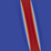
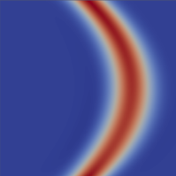
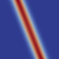
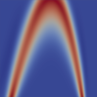
Figure 1: Density matches computed from the manufactured solutions to problem 21 in Table 1. Left to right: example 0 through 3.

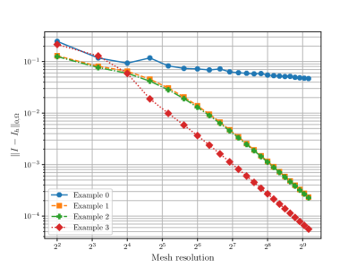
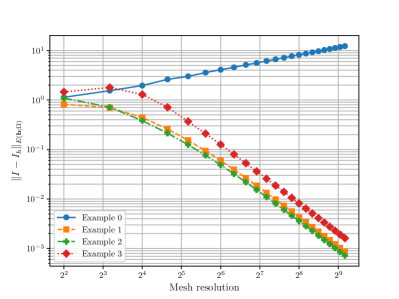
Figure 2: Convergence as a function of mesh resolution $h^{-1}$ for the examples in Table 1. Left: $L^{2}$ errors. Right ${E(\mathbf{b};\Omega)}$ errors.

2.2 Outer Problem

The inner problem equips us with a forward operator that maps the one-parameter family of velocity fields to a solution of the inner problem. These forward operators motivate a gradient descent method to solve the inverse problem of finding the optimal velocity $u$ minimizing the metamorphosis functional (1a).

Central to the preceding analysis was the space ${G(\mathbf{b};\Omega)}$ which depends explicitly on the velocity $u$ via $\mathbf{b}$. If we wish to explore the space ${L^{2}([0,1],V)}$ by means of a gradient descent method perturbing a velocity $u\mapsto u+\delta u$ (where $\delta u$ is some appropriate search direction) implies a change in the Hilbert space ${G(\mathbf{b};\Omega)}$. Since a variation $\delta u$ in the velocity is arbitrary, it is not straight-forward to characterize the derivative of image $I\in{G(\mathbf{b};\Omega)}$ since it surely will not occupy ${G(\mathbf{b};\Omega)}$ unless the variation $\delta u$ vanishes. A practical solution to this problem is therefore simply to restrict the space of images to be continuous everywhere on $\Omega$ by using the conforming discretization (23). The approach we take here is called a discretize-then-optimize strategy, where we replace the function spaces with finite-dimensional surrogates and then apply a gradient descent method. This is in contrast with an optimize-then-discretize scheme, where an optimality system (sometimes referred to as the Karush-Kuhn-Tucker system) is derived for an infinite-dimensional optimisation problem after which the resulting equations are discretized together. We return to this briefly later on, see also [29, Chapter 3] for details.

First we define a semi-discrete version of (2) where the velocity is infinite-dimensional and the solution image occupies the conforming finite element space. This version of the inverse problem is as follows:

$$\inf_{(u,I)\in{L^{2}([0,1],V_{h})}\times G_{h}}\quad H=\frac{1}{2}\int_{0}^{1}\|u\|_{V}^{2}\;\textnormal{d}t+\sigma^{-2}\|\mathbf{b}\cdot\nabla_{t}I^{*}[u]\|_{0,\Omega}^{2}$$ (25a)

subject to $$I^{*}[u]\triangleq\arg\inf_{\begin{subarray}{c}I\in G_{h},\\ I|_{\Gamma_{0}}=I_{0},\\ I|_{\Gamma_{1}}=I_{1}\end{subarray}}\|\mathbf{b}\cdot\nabla_{t}I\|^{2}_{0,\Omega}.$$ (25b)

We write this as a reduced problem for the control variable $u$:

$$\inf_{u\in V}\quad H_{R}=\frac{1}{2}\int_{0}^{1}\|u\|_{V}^{2}\;\textnormal{d}t+\sigma^{-2}\|\mathbf{b}\cdot\nabla_{t}I^{*}[u]\|_{0,\Omega}^{2}$$ (26a)

subject to $$I^{*}[u]\text{ solves problem }\ref{leastsquareadvection}.$$ (26b)

$I^{*}[u]$ is the optimal source term given $u$ in sense of the inner problem. First, we note that (25) and (26) lead to the same stationary points, so the reformulation is idempotent. Indeed, setting $\delta H=0$ yields:

$$\int_{0}^{1}\langle u,\delta u\rangle_{V}\;\textnormal{d}t=-\sigma^{-2}\langle\mathbf{b}\cdot\nabla_{t}I,\delta u\cdot\nabla I\rangle_{0,\Omega},\quad \forall\delta u\in{L^{2}([0,1],V)},$$

$$\langle\mathbf{b}\cdot\nabla I,\mathbf{b}\cdot\nabla\delta I\rangle_{0,\Omega}=0,\quad \forall\delta I\in G_{h},$$

with the image at time $t=0,1$ fixed. Since $G_{h}$ is a globally continuous piecewise finite-dimensional space, the spatial derivative is well-defined in a weak sense. Carrying out the same steps for $H_{R}$ we get:

$$\int_{0}^{1}\langle u,\delta u\rangle_{V}\;\textnormal{d}t=-\sigma^{-2}\langle\mathbf{b}\cdot\nabla_{t}I^{*}[u],\mathbf{b}\cdot\nabla_{t}\frac{\delta I^{*}}{\delta u}[u]\delta u+\delta u\cdot\nabla I^{*}[u]\rangle_{0,\Omega},\quad \forall\delta u\in{L^{2}([0,1],V)},$$ (27)

where $\frac{\delta I^{*}}{\delta u}[u]\delta u$ is the sensitivity of $I^{*}[u]$ at $u$ with respect to $u$. We notice that the reduced nature of the reformulation (26) introduces a new term in the equation for $u$. However, since $\frac{\delta I^{*}}{\delta u}[u]\delta u\in G_{h}$ (since the variational derivative is taken in sense of Fréchet), then:

$$\langle\mathbf{b}\cdot\nabla_{t}I^{*}[u],\mathbf{b}\cdot\nabla_{t}\frac{\delta I^{*}}{\delta u}[u]\rangle_{0,\Omega}=0,$$

since $I^{*}[u]$ solves problem 21, which is a convex problem, so the equivalence follows.

Equipped with a reduced problem we now discretise the space of the velocity field. The norm in (4) is equivalent to an $H^{3}$ norm in space in line with assumption 2.1. Ideally, this property must be preserved under discretization, independently of the mesh refinement parameter. An $H^{3}$ conforming finite element space is globally $\mathsf{C}^{2}$ and an implementation is, to the best of the authors’ knowledge, not available. In this paper we focus our mathematical analysis on the inner problem and in this section concentrate our work on developing and implementing a gradient descent scheme on the velocity field. Deferring convergence analysis pertaining to the velocity field to future work we therefore discretize the velocity field by continuous piecewise affine functions. In practice we use the iterated nature of the operator $L$ in (4) and solve a modified version of (26) as follows. Using the space-time bilinear form:

$$a(w,v)=\langle w,v\rangle_{0,\Omega}+\alpha^{2}\langle\nabla w,\nabla v\rangle_{0,\Omega},$$

this version given by (28) below:

$$\inf_{v_{h}^{0}\in\mathcal{P}^{1}(\Omega_{h})}\quad H_{R}=\frac{1}{2}\|v_{h}^{0}\|_{0,\Omega}^{2}+\sigma^{-2}\|\mathbf{b}\cdot\nabla_{t}I_{h}^{*}[u_{h}]\|_{0,\Omega}^{2}$$ (28a)

subject to $$G_{h}\ni I_{h}^{*}[u_{h}]\text{ solves problem }\ref{leastsquareadvection:disc},$$ (28b)

$$a(v^{1}_{h},w)=\langle v_{h}^{0},w\rangle_{0,\Omega},\quad\forall w\in\mathcal{P}^{1}(\Omega_{h}),$$ (28c)

$$a(v_{h}^{2},w)=\langle v_{h}^{1},w\rangle_{0,\Omega},\quad\forall w\in\mathcal{P}^{1}(\Omega_{h}),$$ (28d)

$$a(u_{h},w)=\langle v_{h}^{2},w\rangle_{0,\Omega},\quad\forall w\in\mathcal{P}^{1}(\Omega_{h}),$$ (28e)

where $\mathcal{P}^{1}(\Omega_{h})$ is a $\mathsf{C}^{0}$ conforming finite element space consisting of piecewise affine functions defined over the mesh $\Omega$. Although this precludes $u_{h}$ from having a mesh-independent Lipschitz constant, (28) forms the basis for a useful numerical method. The next section discusses how this can be realized numerically using the Firedrake software package [46] as well as how knowledge of the existence of the gradient from the previous section motivates an adjoint-based automatic differentiation algorithm.

2.3 Numerical Examples

Automatic differentiation is a software abstraction allowing for the numerical evaluation of the Jacobian of expressions that are given as functions in a programming language, see [42]. These essentially articulate chain and product rules for computer programmes. The implementation of such an abstraction permits a user to evaluate gradients of for instance complex composite functions for use in an optimisation loop. For instance, formally speaking, the derivative of the functional in (26) with respect to the velocity requires some sense to be made about the expression $\frac{\delta z^{*}[u]}{\delta u}$. In the PDE-constrained optimisation community this expression is called the adjoint and it is precisely the machinery of automatic differentiation that (upon suitable discretization) allows for its numerical evaluation. This machinery is indeed necessary as no explicit gradient can be evaluated from $z^{*}[u]$. Firedrake supports an automatic differentiation engine (see [41]) so with only a few lines of code expresses the optimisation problem (26) which can then be solved by e.g. a Broyden-Fletcher-Goldfarb-Shanno (BFGS) algorithm [44] (we used the Rapid Optimization Library (ROL), see trilinos.github.io). Here we provide but a few numerical examples to support our work in section 2.1.2.

Figures 3–4 show the image (or density) $I$ results of a gradient descent applied to the problem in (26) using Firedrake’s automatic differentiation abstraction and the conforming discretization from section 21. In these figures, $h=0.0125$. Both the image and the velocity field is discretized using a globally continuous piecewise linear finite element space on a spatially periodic domain. These figures show that our method is able to compute meaningful matches between different densities. In Fig. 3.A and E we see that transport solutions are recovered, even in the presence of a template with a sharp spatial gradient. For the other cases we have chosen densities which can be matched without pure transport. In some instances, i.e. F and D, the gradient descent finds intuitive matches between the data, while B, C and G struggle to recover the same visual effect. For these three configurations we find that advection is recovered for some parts of the image but we do not see a merging effect as before. For instance, in Fig. 3.C it is more economical to seek an approximately constant velocity field to match the left-most mode of the template while causing the right-most mode to vanish.

We also comment on the role of $\sigma$ which we recall acts as a penalisation parameter for advection term. In Fig. 3 the two terms in (26) are weighted equally. Figure 4 uses the same data as in Fig. 3, albeit with $\sigma^{-2}=10^{5}$. We observe similar results as before with the exception of B and C. Adjusting the value of the penalty parameter allows the gradient method to recover, with moderate success, some of the density merging behaviour observed previously. With a more complete theoretical understanding of the space-time gradient descent method, and more expertise in numerical optimisation, we can begin to carry out more careful parameter studies for $\sigma$. This is deferred to future work.

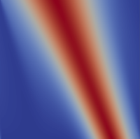
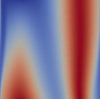
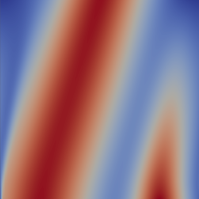
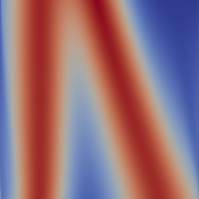
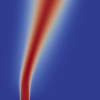
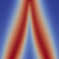
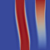
Figure 3: Results for the outer problem for various template and target pairs in one dimension. The vertical dimension is time and the horizontal dimension is space, so the north and south faces of the domain represent the target and template, respectively. Here we have taken $\sigma^{-2}=1$.

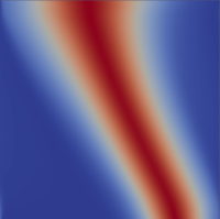
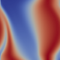
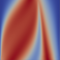
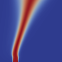
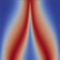
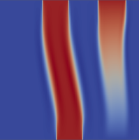
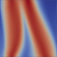
Figure 4: Results for the outer problem for various template and target pairs in one dimension with the same template and target densities as in Fig. 4. Here we have taken $\sigma^{-2}=10^{5}$ thereby forcing the algorithm to seek more diffeomorphic geodesics.

We also present some results for $d=2$ in Fig. 5 and 6 for different values of $\sigma$. Here we use the boundary conditions $u_{t}|_{\partial{\omega}}=0$, $\forall t\in[0,1]$, meaning that there is no inflow or outflow boundaries in space. In the spatial dimension, $h=0.0125$ and extruded in time with $15$ subdivisions. The observations are similar to those in the one-dimensional case. We comment on a few of these. For transport-type problems (the first and third rows of Figs. 5–6), the parameter $\sigma$ does not change the nature of the solutions, albeit smearing out the smooth data in the first row when the penalty parameter is low. This behaviour is not present for discontinuous data which we attribute the flow being almost grid-aligned and constant in time. $\sigma$ does not appear to alter the merging effect in the example provided in the second row of the figures, though overall the intensity values are lower whenever $\sigma=1$. Again this can be explained by advection being enforced to a lesser extent, but not changing the direction of the velocity field. Lastly are the fourth and fifth rows where we truly see the influence of $\sigma$. When $\sigma=1$ in Fig. 5, very little advection is observed and the motion between the template and the target can be viewed as a simple ”fading in/out” effect. In Fig. 6, however, we see some interesting results showing more meaningful (qualitatively speaking), geodesics between the images. Although these results are still of a toy problem nature they show clear promise for our approach. These results can be generated in less than 24 hours on standard consumer hardware (without using any preconditioning whatsoever). Applying high performance parallel algorithms are the subject of future research.

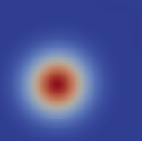
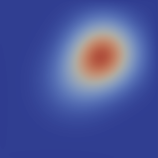
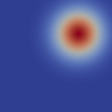
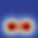
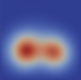
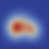
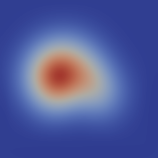
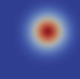
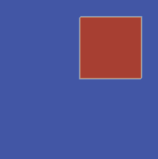
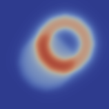
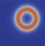
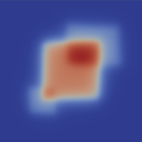
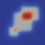
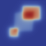
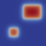
Figure 5: Results for the outer problem for various template and target pairs in two dimensions for $\sigma^{-2}=1$. Each row shows the evolution at time $t=0,0.25,0.5,0.75,1$.

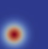
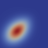
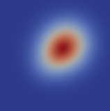
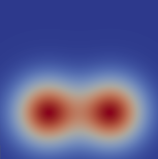
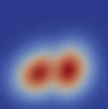
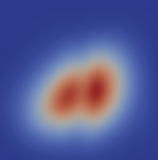
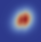
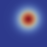
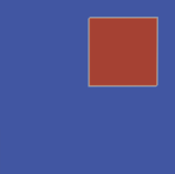
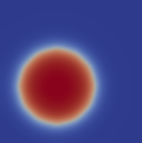
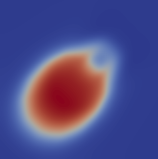
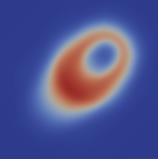
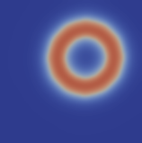
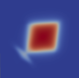
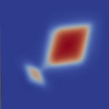
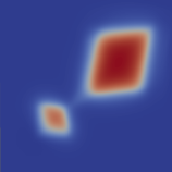
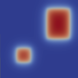
Figure 6: Results for the outer problem for various template and target pairs in two dimensions for $\sigma^{-2}=10^{5}$ to seek more diffeomorphic geodesics. Each row shows the evolution at time $t=0,0.25,0.5,0.75,1$.

3 Summary

We successfully cast the metamorphosis problem in a variational Hilbertian space-time setting. The variational setting introduced in section 2.1 provides a novel framework to study weakly space-time $\mathbf{b}\cdot\nabla_{t}$-differentiable geodesics for metamorphosis. A primal least-squared formulation was studied and we showed several theoretical results for the inner problem. Based on this we presented a simple conforming finite element method. Section 2.2 showed a practical adjoint-based way to solve the inverse problem to find a suitable velocity field $u$ requiring minimal implementation effort by the user.

There are many open problems and options yet to be explored for space-time metamorphosis. The main theoretical challenges for the inner problem is showing a regularity result akin to the usual elliptic regularity for $H^{1}$ variational problems. Preconditioning of the least-squared system in section 2.1.2 is another option for future research, as is the investigation of weaker notions of discretizations e.g. using the discontinuous Petrov-Galerkin framework, see [17]. The work of [1] offers some insights into preconditioning for a space-time wave equation and offers excellent numerical evidence that might be useful in this endeavour. Space-time adaptivity could also be explored in order to resolve details of images represented as finite element functions, in which case one would dispense with a quasi-uniformity assumption on the mesh. In view of our numerical experiments for $d=2$ we believe this paper provides the basis for a powerful method given good preconditioners and more bespoke numerical optimizers.
The outer problem also presents some possibilities for future work. As mentioned, a conforming finite element discretization of $V$ is desirable, although a $\mathsf{C}^{0}$ conforming $H^{3}$ non-conforming finite element exists and could be explored, see [53]. Since the Lipschitz regularity of the velocity field is only required in space, such an implementation over the spatial domain could be combined with extruded quadrilateral meshes to impose different temporal and spatial regularity, see [38, 8].
In this project we have chosen to treat the outer problem with a discretize-then-optimize approach because of the availability of the seamless adjoint framework in Firedrake. Another approach that was attempted was to derive the Euler-Lagrange equations for the ”full” metamorphosis problem (also called EPDiff in the literature) to solve for $u$, $I$ and $z$ simultaneously, and then discretize this non-linear system of equations. A Newton method could then be applied for this system. Some work has been done previously in this area for LDDMM, see [28]. Also, the work [56] establishes a fast algorithm for computing finite-dimensional velocity fields which could be used in conjunction with the inner problem formulations above. This may be morally similar to discretizing the velocity field using finite elements but we simply mention this as a possible avenue owing to the numerical evidence in support of the authors’ work.

Appendix A. Inner Problem Convergence Results for $d=1$

Table 2: Convergence rates for example 0 from Table 1

$h^{-1}$

Table 3: Convergence rates for example 1 from Table 1

$h^{-1}$

Table 4: Convergence rates for example 2 from Table 1

$h^{-1}$

Table 5: Convergence rates for example 3 from Table 1

$h^{-1}$

Appendix B. Inner Problem Convergence Results for $d=2$

We also construct a test suite for $d=2$ for some simple advection problems. Table 6 shows these manufactured solutions with convergence rates shown in Table Appendix B. Inner Problem Convergence Results for $d=2$, Appendix B. Inner Problem Convergence Results for $d=2$ and Appendix B. Inner Problem Convergence Results for $d=2$. These rates are also depicted in Fig. 7.

Table 6: Manufactured solutions to (21) where $d=2$

No.	$I(x,t)$	$u(x,t)$
0	$e^{-25((x-0.3(1-t)-0.6t)^{2}+(y-0.3(1-t)-0.6t)^{2})}$	$(0.3,0.3)$
1	$e^{-25((x-0.3(1-t)-0.7t)^{2}+(y-0.5)^{2})}$	$(0.4,0)$
2	$e^{-25((y-0.3(1-t)-0.7t)^{2}+(x-0.5)^{2})}$	$(0,0.4)$

Table 7: Convergence rates for example 0 from Table 6

$h^{-1}$

Table 8: Convergence rates for example 1 from Table 6

$h^{-1}$

Table 9: Convergence rates for example 2 from Table 6

$h^{-1}$

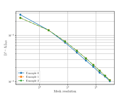
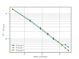
Figure 7: Convergence as a function of mesh resolution $h^{-1}$ for the examples in Table 6. Left: $L^{2}$ errors. Right ${E(\mathbf{b};\Omega)}$ errors.

References

- [1] M. Anderson and J.-H. Kimn. A numerical approach to space-time finite elements for the wave equation. Journal of Computational Physics, 226(1):466–476, 2007.
- [2] V. I. Arnold. Sur la géométrie différentielle des groupes de Lie de dimension infinie et ses applications à l’hydrodynamique des fluides parfaits. Ann. Inst. Fourier, 16(1):319–361, 1966.
- [3] R. Bajcsy and S. Kovačič. Multiresolution elastic matching. Computer vision, graphics, and image processing, 46(1):1–21, 1989.
- [4] M. Bauer, M. Bruveris, and P. W. Michor. Overview of the geometries of shape spaces and diffeomorphism groups. Journal of Mathematical Imaging and Vision, 50(1-2):60–97, 2014.
- [5] M. F. Beg and A. Khan. Computing an average anatomical atlas using LDDMM and geodesic shooting. In 3rd IEEE International Symposium on Biomedical Imaging: Nano to Macro, 2006., pages 1116–1119. IEEE, 2006.
- [6] M. F. Beg, M. I. Miller, A. Trouvé, and L. Younes. Computing large deformation metric mappings via geodesic flows of diffeomorphisms. International Journal of Computer Vision, 61(2):139–157, 2005.
- [7] T. Beier and S. Neely. Feature-based image metamorphosis. ACM SIGGRAPH computer graphics, 26(2):35–42, 1992.
- [8] G.-T. Bercea, A. T. McRae, D. A. Ham, L. Mitchell, F. Rathgeber, L. Nardi, F. Luporini, and P. H. Kelly. A structure-exploiting numbering algorithm for finite elements on extruded meshes, and its performance evaluation in Firedrake. arXiv preprint arXiv:1604.05937, 2016.
- [9] P. Bochev and J. Choi. Improved least-squares error estimates for scalar hyperbolic problems. Computational Methods in Applied Mathematics Comput. Methods Appl. Math., 1(2):115–124, 2001.
- [10] P. B. Bochev and M. D. Gunzburger. Least-squares finite element methods, volume 166. Springer Science & Business Media, 2009.
- [11] S. K. Boyd. Image-based finite element analysis. In Advanced Imaging in Biology and Medicine, pages 301–318. Springer, 2009.
- [12] S. Brenner and R. Scott. The Mathematical Theory of Finite Element Methods, volume 15. Springer Science & Business Media, 2007.
- [13] M. Bruveris. Riemannian geometry for shape analysis and computational anatomy. arXiv preprint arXiv:1807.11290, 2018.
- [14] A. J. Chorin, J. E. Marsden, and J. E. Marsden. A mathematical introduction to fluid mechanics, volume 3. Springer, 1990.
- [15] G. E. Christensen, R. D. Rabbitt, and M. I. Miller. Deformable templates using large deformation kinematics. IEEE transactions on image processing, 5(10):1435–1447, 1996.
- [16] H. De Sterck, T. A. Manteuffel, S. F. McCormick, and L. Olson. Least-squares finite element methods and algebraic multigrid solvers for linear hyperbolic PDEs. SIAM Journal on Scientific Computing, 26(1):31–54, 2004.
- [17] L. Demkowicz and J. Gopalakrishnan. A class of discontinuous Petrov–Galerkin methods. part i: The transport equation. Computer Methods in Applied Mechanics and Engineering, 199(23-24):1558–1572, 2010.
- [18] Y. Dong. Prescribing the Jacobian determinant in Sobolev spaces. In Annales de l’Institut Henri Poincare (C) Non Linear Analysis, volume 11, pages 275–296. Elsevier, 1994.
- [19] J. Du, L. Younes, and A. Qiu. Whole brain diffeomorphic metric mapping via integration of sulcal and gyral curves, cortical surfaces, and images. NeuroImage, 56(1):162–173, 2011.
- [20] P. Dupuis, U. Grenander, and M. I. Miller. Variational problems on flows of diffeomorphisms for image matching. Quarterly of Applied Mathematics, pages 587–600, 1998.
- [21] A. Effland, M. Rumpf, and F. Schäfer. Image extrapolation for the time discrete metamorphosis model - existence and applications. arXiv preprint arXiv:1705.04490, 2017.
- [22] A. Ern and J.-L. Guermond. Theory and practice of finite elements, volume 159. Springer Science & Business Media, 2013.
- [23] B. Fischer and J. Modersitzki. Ill-posed medicine - an introduction to image registration. Inverse Problems, 24(3):34008, 2008.
- [24] U. Grenander. General pattern theory, 1993.
- [25] U. Grenander and M. I. Miller. Representations of knowledge in complex systems. Journal of the Royal Statistical Society. Series B (Methodological), pages 549–603, 1994.
- [26] U. Grenander and M. I. Miller. Pattern theory: from representation to inference. Oxford University Press, 2007.
- [27] A. Günther, H. Lamecker, and M. Weiser. Direct LDDMM of discrete currents with adaptive finite elements. 2011.
- [28] M. Hernandez and S. Olmos. Gauss-Newton optimization in diffeomorphic registration. In 2008 5th IEEE International Symposium on Biomedical Imaging: From Nano to Macro, pages 1083–1086. IEEE, 2008.
- [29] M. Hinze, R. Pinnau, M. Ulbrich, and S. Ulbrich. Optimization with PDE constraints, volume 23. Springer Science & Business Media, 2008.
- [30] D. D. Holm, A. Trouvé, and L. Younes. The Euler-Poincaré theory of metamorphosis. Quarterly of Applied Mathematics, pages 661–685, 2009.
- [31] P. Houston, J. A. Mackenzie, E. Süli, and G. Warnecke. A posteriori error analysis for numerical approximations of Friedrichs systems. Numerische Mathematik, 82(3):433–470, 1999.
- [32] P. Houston, R. Rannacher, and E. Süli. A posteriori error analysis for stabilised finite element approximations of transport problems. Computer methods in applied mechanics and engineering, 190(11-12):1483–1508, 2000.
- [33] T. J. Hughes and G. M. Hulbert. Space-time finite element methods for elastodynamics: formulations and error estimates. Computer methods in applied mechanics and engineering, 66(3):339–363, 1988.
- [34] G. M. Hulbert and T. J. Hughes. Space-time finite element methods for second-order hyperbolic equations. 1990.
- [35] U. E. Langer and O. S. (Ed.). Space-Time Methods. Applications to Partial Differential Equations. De Gruyter, 2019.
- [36] T. A. Manteuffel, K. J. Ressel, and G. Starke. A boundary functional for the least-squares finite-element solution of neutron transport problems. SIAM Journal on Numerical Analysis, 37(2):556–586, 1999.
- [37] C. R. Maurer and J. M. Fitzpatrick. A review of medical image registration. Interactive Image-guided Neurosurgery, 17, 1993.
- [38] A. T. McRae, G.-T. Bercea, L. Mitchell, D. A. Ham, and C. J. Cotter. Automated generation and symbolic manipulation of tensor product finite elements. SIAM Journal on Scientific Computing, 38(5):S25–S47, 2016.
- [39] M. I. Miller, A. Trouvé, and L. Younes. On the metrics and Euler-Lagrange equations of computational anatomy. Annual Review of Biomedical Engineering, 4(1):375–405, 2002.
- [40] M. I. Miller and L. Younes. Group actions, homeomorphisms, and matching: A general framework. International Journal of Computer Vision, 41(1-2):61–84, 2001.
- [41] S. Mitusch, S. Funke, and J. Dokken. dolfin-adjoint 2018.1: automated adjoints for fenics and firedrake. Journal of Open Source Software, 4(38):1292, 2019.
- [42] U. Naumann. The art of differentiating computer programs: an introduction to algorithmic differentiation, volume 24. Siam, 2012.
- [43] H. Nguyen and J. Reynen. A space-time least-square finite element scheme for advection-diffusion equations. Computer Methods in Applied Mechanics and Engineering, 42(3):331–342, 3 1984.
- [44] J. Nocedal and S. Wright. Numerical optimization. Springer Science & Business Media, 2006.
- [45] P. Perrochet and P. Azérad. Space-time integrated least-squares: Solving a pure advection equation with a pure diffusion operator. Journal of computational physics, 117(2):183–193, 1995.
- [46] F. Rathgeber, D. A. Ham, L. Mitchell, M. Lange, F. Luporini, A. T. McRae, G.-T. Bercea, G. R. Markall, and P. H. Kelly. Firedrake: automating the finite element method by composing abstractions. ACM Transactions on Mathematical Software (TOMS), 43(3):1–27, 2016.
- [47] W. Sickel and A. Youssfi. The characterisation of the regularity of the Jacobian determinant in the framework of potential spaces. Journal of the London Mathematical Society, 59(1):287–310, 1999.
- [48] A. Trouvé. An infinite dimensional group approach for physics based models in pattern recognition. Preprint, 1995.
- [49] A. Trouvé. Diffeomorphisms groups and pattern matching in image analysis. International Journal of Computer Vision, 28(3):213–221, 1998.
- [50] A. Trouvé and L. Younes. Local geometry of deformable templates. SIAM Journal on Mathematical Analysis, 37(1):17–59, 2005.
- [51] A. Trouvé and L. Younes. Metamorphoses through Lie group action. Foundations of Computational Mathematics, 5(2):173–198, 2005.
- [52] L. Wang, F. Beg, T. Ratnanather, C. Ceritoglu, L. Younes, J. C. Morris, J. G. Csernansky, and M. I. Miller. Large deformation diffeomorphism and momentum based hippocampal shape discrimination in dementia of the alzheimer type. IEEE transactions on medical imaging, 26(4):462–470, 2007.
- [53] S. Wu and J. Xu. Nonconforming finite element spaces for th order partial differential equations on simplicial grids when . Mathematics of Computation, 88(316):531–551, 2019.
- [54] L. Younes. Shapes and diffeomorphisms, volume 171. Springer Science & Business Media, 2010.
- [55] Software used in ’Space-time metamorphosis’, April 2020. https://doi.org/10.5281/zenodo.3778236.
- [56] M. Zhang and P. T. Fletcher. Finite-dimensional Lie algebras for fast diffeomorphic image registration. In International Conference on Information Processing in Medical Imaging, pages 249–260. Springer, 2015.