Higher-order level spacings in random matrix theory based on Wigner’s conjecture

Abstract

The distribution of higher order level spacings, i.e. the distribution of $\{s_{i}^{(n)}=E_{i+n}-E_{i}\}$ with $n\geq 1$ is derived analytically using a Wigner-like surmise for Gaussian ensembles of random matrix as well as Poisson ensemble. It is found $s^{(n)}$ in Gaussian ensembles follows a generalized Wigner-Dyson distribution with rescaled parameter $\alpha=\nu C_{n+1}^{2}+n-1$, while that in Poisson ensemble follows a generalized semi-Poisson distribution with index $n$. Numerical evidences are provided through simulations of random spin systems as well as non-trivial zeros of Riemann zeta function. The higher order generalizations of gap ratios are also discussed.

I Introduction

Random matrix theory (RMT) was introduced half a century ago when dealing with complex nucleiPorter , and since then has found various applications in fields ranging from quantum chaos to isolated many-body systemsRMP ; PR . This roots in the fact that RMT describes universal properties of random matrix that depend only on its symmetry while independent of microscopic details. Specifically, the system with time reversal invariance is represented by matrix that belongs to the Gaussian orthogonal ensemble (GOE); the system with spin rotational invariance while breaks time reversal symmetry belongs to the Gaussian unitary ensemble (GUE); while Gaussian symplectic ensemble (GSE) represents systems with time reversal symmetry but breaks spin rotational symmetry.

Among various statistical quantities, the most widely used one is the distribution of nearest level spacings $\left\{s_{i}=E_{i+1}-E_{i}\right\}$, i.e. the gaps between adjacent energy levels, which measures the strength of level repulsion. The exact expression for the $P\left(s\right)$ can be derived analytically for random matrix with large dimension, which is cumbersomeMehta ; Haake2001 . Instead, for most practical purposes it’s sufficient to employ the so-called Wigner surmiseWigner that deals with $2\times 2$ matrix (this will be reviewed in Sec. II), the out-coming result for $P(s)$ has a neat expression that contains a polynomial part accounting for level repulsion and an Gaussian decaying part (see Eq. (6)).

Different models may and usually do have different density of states (DOS), hence to compare the universal behavior of level spacings, an unfolding procedure is required to erase the model dependent information of DOS. To overcome this obstacle, Oganesyan and HuseOganesyan proposed a new quantity to study the level statistics, i.e. the ratio between adjacent gaps $\left\{r_{i}=s_{i+1}/s_{i}\right\}$, whose distribution $P\left(r\right)$ is later analytically derived by Atas et al.Atas . The gap ratio is independent of local DOS and requires no unfolding procedure (provided the DOS does not vary in the scale of the spacings involve), hence has found various applications, especially in the context of many-body localization (MBL)Huse1 ; Huse2 ; Huse3 ; Sarma ; Lev ; Agarwal ; Luitz ; Avishai2002 ; Regnault16 ; Regnault162 .

Both the nearest level spacing and gap ratio account for the short range level correlations. However, long range correlations are also important, especially when studying the MBL transition phenomena. Indeed, there’re several effective models describing the level distribution at the MBL transition region. For example, the Rosenzweig-Porter modelShukla , mean field plasma modelSerbyn , short-range plasma models (SRPM)SRPM and its generalization – so-called weighed SRPMSierant19 , Gaussian $\beta$ ensembleBuijsman and the generalized $\beta-h$ modelSierant20 . All of these models more or less describe the short-range level correlations in the MBL transition region well, and their difference can only be revealed when long-range correlations are concerned. For a comparison of these models in describing MBL transition point, see Ref. [Sierant19, ].

Commonly, the long-range correlations in a random matrix can be described by the number variance $\Sigma^{2}$ or the Dyson-Mehta $\Delta_{3}$ statisticsHaake2001 , however, both of them are very sensitive to the concrete unfolding strategy and have already been a source of misleading signaturesGomez2002 . Instead, it’s more direct and numerically easier to study the higher order level spacings and gap ratios. There’re existing works that generalize the level spacing and gap ratios to higher order, as well as their applications in studying MBL transitionsSierant19 ; Sierant20 ; Tekur1 ; Tekur ; Atas2 ; Chavda ; Magd ; Duras ; Rubah . However, most of these works are numerical or phenomenological, and an analytical derivation for the distribution of level spacing/gap ratio is still lacking. Given the importance of higher-order level correlations, it’s desirable to have an analytical formula for them, it is then the purpose of this work to fill in this gap.

In this work, by using a Wigner-like surmise, we succeeded in obtaining an analytical expression for the distribution of higher order spacing $\left\{s_{i}^{\left(n\right)}=E_{i+n}-E_{i}\right\}$ in all the Gaussian ensembles of RMT, as well as the Poisson ensemble. The results show the distribution of $s_{i}^{\left(n\right)}$ in the former class follows a generalized Wigner-Dyson distribution with rescaled parameter; while in Poisson ensemble it follows a generalized semi-Poisson distribution with index $n$. Interestingly, the rescaling behavior of higher-order level spacing is identical to that of the high-order gap ratio found numerically in Ref. [Tekur, ], for which we will provide a heuristic explanation.

This paper is organized as follows. In Sec. II we review the Wigner surmise for deriving the distribution of nearest level spacings, and present numerical data to validate this surmise. In Sec. III.1 we present the analytical derivation for higher order level spacings using a Wigner-like surmise, and numerical fittings are given in Sec. III.2. In Sec. IV we discuss the generalization of gap ratios to higher order. Conclusion and discussion come in Sec. V.

II Nearest Level Spacings

We begin with the discussion about nearest level spacings, our starting point probability distribution of energy levels $P\left(\left\{E_{i}\right\}\right)$ in three Gaussian ensembles, whose expression can be found in any textbook on RMT (e.g. Ref. [Haake2001, ]),

$$P\left(\left\{E_{i}\right\}\right)\propto\prod_{i<j}\left|E_{i}-E_{j}\right|^{\nu}e^{-A\sum_{i}E_{i}^{2}}$$ (1)

where $\nu=1,2,4$ for GOE,GUE,GSE respectively. The distribution of nearest level spacing can then be written as

$$P\left(s\right)=\int\prod_{i=1}^{N}dE_{i}P\left(\left\{E_{i}\right\}\right)\delta\left(s-\left|E_{1}-E_{2}\right|\right)\text{,}$$ (2)

where $N$ is the number of levels in $\left\{E_{i}\right\}$ and the analytical result is quite complicated for general $N$. Instead, Wigner proposes a surmise that we can focus on the $N=2$ case, the distribution then reduces to

$$P\left(s\right)\propto\int_{-\infty}^{\infty}\left|E_{1}-E_{2}\right|^{\nu}\delta\left(s-\left|E_{1}-E_{2}\right|\right)e^{-A\sum_{i}E_{i}^{2}}dE_{1}dE_{2}\text{.}$$ (3)

By introducing $x_{1}=E_{1}-E_{2}$, $x_{2}=E_{1}+E_{2}$, we have

$$P\left(s\right) \propto 2\int_{-\infty}^{\infty}\left|x_{1}\right|^{\nu}\delta\left(s-\left|x_{1}\right|\right)e^{-\frac{A}{2}\sum_{i}x_{i}^{2}}dx_{1}dx_{2}$$ (4)

$$= Cs^{\nu}e^{-As^{2}/2}\text{.}$$

The constants $A,C$ can be determined by working out the integral about $x_{2}$, but it is more convenient to obtain by imposing the normalization condition

$$\int_{0}^{\infty}P\left(s\right)ds=1\text{, }\int_{0}^{\infty}sP\left(s\right)ds=1\text{.}$$ (5)

From which we can reach to the celebrated Wigner-Dyson distribution

$$P(s)=\left\{\begin{array}[]{ll}\frac{\pi}{2}s\exp\big{(}-\frac{\pi}{4}s^{2}\big{)}&\nu=1\quad\text{GOE}\\[2.84526pt] \frac{32}{\pi^{2}}s^{2}\exp\big{(}-\frac{4}{\pi}s^{2}\big{)}&\nu=2\quad\text{GUE}\\[2.84526pt] \frac{2^{18}}{3^{6}\pi^{3}}s^{4}\exp\big{(}-\frac{64}{9\pi}s^{2}\big{)}&\nu=4\quad\text{GSE}\end{array}\right.$$ (6)

On the other hand, the levels are independent in Poisson ensemble, which means the occurrence of next level is independent of previous level, the nearest level spacings then follows a Poisson distribution $P\left(s\right)=\exp\left(-s\right)$.

Although the Wigner surmise is for $2\times 2$ matrix, it works fairly good when the matrix dimension is large. To demonstrate this, we present numerical evidence from a quantum many-body system – the spin-$1/2$ Heisenberg model with random external field, which is the canonical model in the study of many-body localization (MBL), whose Hamiltonian in a length-$L$ chain is

$$H=\sum_{i=1}^{L}\mathbf{S}_{i}\cdot\mathbf{S}_{i+1}+\sum_{i=1}^{L}\sum_{\alpha=x,y,z}h^{\alpha}\varepsilon_{i}^{\alpha}S_{i}^{\alpha},$$ (7)

where we set coupling strength to be $1$ and assume periodic boundary condition in Heisenberg term. The $\varepsilon_{i}^{\alpha}$’s are random numbers within range $\left[-1,1\right]$, and $h^{\alpha}$ is referred as the randomness strength. We focus on two choices of $h^{\alpha}$: (i) $h^{x}=h^{z}=h\neq 0$ and $h^{y}=0$, the Hamiltonian matrix is orthogonal; (ii) $h^{x}=h^{y}=h^{z}=h\neq 0$, the model being unitary. This model undergos a thermal-MBL transition at roughly $h_{c}\simeq 3$ ($2.5$) in the orthogonal (unitary) model, where the level spacing distribution evolves from GOE (GUE) to PoissonRegnault16 .

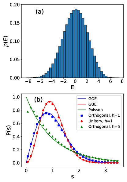
Figure 1: (a) The density of states (DOS) $\rho(E)$ of random field Heisenberg model at $L=12$ and $h=1$ in orthogonal case, the DOS is more uniform in the middle part, we therefore choose the middle half levels to do level statistics. (b) Distribution of nearest level spacings $P(E_{i+1}-E_{i})$, we see a GOE/GUE distribution for $h=1$ in the orthogonal/unitary model, while a Poisson distribution is found for $h=5$ in orthogonal model, the result for $h=5$ in unitary model is not displayed since it coincides with that in the orthogonal model.

We choose a $L=12$ system to present a numerical simulation, and prepare $500$ samples at $h=1$ and $h=5$ for both the orthogonal and unitary model. In Fig. 1(a) we plot the density of states (DOS) for the $h=1$ case in orthogonal model. We can see DOS is much more uniform in the middle part of the spectrum, which is also the case for $h=5$ and unitary model. Therefore we choose the middle half of energy levels to do the spacing counting, and the results are shown in Fig. 1(b). We observe a clear GOE/GUE distribution for $h=1$ in orthogonal/unitary model and a Poisson distribution for $h=5$ in orthogonal model as expected, the fitting result for $h=5$ in unitary model is not shown since it almost coincides with that in orthogonal model. It is noted the fitting for Poisson distribution has minor deviations around the region $s\sim 0$, this is due to finite size effect since there will always remain exponentially-decaying but finite correlation between levels in a finite system. As we will demonstrate in subsequent section, the fitting for higher order level spacings will be better since the overlap between levels decays exponentially with their distance in MBL phase.

A technique issue is, when counting the level spacings, we choose to take the middle half levels of the spectrum, while we can also employ a unfolding procedure using a spline interpolation that incorporates all energy levelsAvishai2002 , and the fitting results are almost the sameRegnault162 ; Rao182 .

III Higher Order Level Spacings

Now we proceed to consider the distribution of higher order level spacings $\left\{s_{i}^{\left(n\right)}=E_{i+n}-E_{i}\right\}$, using a Wigner-like surmise. We first give the analytical derivation, then provide numerical evidence from simulation of spin model in Eq. (7) as well as the non-trivial zeros of Riemann zeta function.

III.1 Analytical Derivation

Introduce $P_{n}\left(s\right)=P\left(s^{\left(n\right)}=s\right)\equiv P\left(\left|E_{i+n}-E_{i}\right|=s\right)$, to apply the Wigner surmise, we are now considering $\left(n+1\right)\times\left(n+1\right)$ matrices, the distribution $P_{n}(s)$ then goes to

$$P_{n}\left(s\right) \propto \int_{-\infty}^{\infty}\prod_{i<j}\left|E_{i}-E_{j}\right|^{\nu}\delta\left(s-\left|E_{1}-E_{n+1}\right|\right)$$ (8)

$$\times e^{-A\sum_{i=1}^{n+1}E_{i}^{2}}\prod_{i=1}^{n+1}dE_{i}$$

We first change the variables to

$$x_{i}=E_{i}-E_{i+1}\text{, }i=1,2,...,n\text{; }\quad x_{n+1}=\sum_{i=1}^{n+1}E_{i}\text{,}$$ (9)

the $P_{n}\left(s\right)$ then evolves into

$$P_{n}\left(s\right)\propto\int_{-\infty}^{\infty}\frac{\partial\left(E_{1},E_{2},...,E_{n+1}\right)}{\partial\left(x_{1},x_{2},...,x_{n+1}\right)}\left(\prod_{i=1}^{n}\prod_{j=i}^{n}\left|\sum_{k=i}^{j}x_{k}\right|^{\nu}\right)\delta\left(s-\left|\sum_{i=1}^{n}x_{i}\right|\right)e^{-\frac{A}{n}\left[\sum_{i=1}^{n}\sum_{j=i}^{n}\left(\sum_{k=i}^{j}x_{k}\right)^{2}+x_{n+1}^{2}\right]}\prod_{i=1}^{n+1}dx_{i}.$$ (10)

In this expression, the Jacobian $\frac{\partial\left(E_{1},E_{2},...,E_{n+1}\right)}{\partial\left(x_{1},x_{2},...,x_{n+1}\right)}$ and integral for $x_{n+1}$ are all constants that can be absorbed into the normalization factor, hence we can simplify $P_{n}\left(s\right)$ to

$$P_{n}\left(s\right) \propto \int_{-\infty}^{\infty}\left(\prod_{i=1}^{n}\prod_{j=i}^{n}\left|\sum_{k=i}^{j}x_{k}\right|^{\nu}\right)\delta\left(s-\left|\sum_{i=1}^{n}x_{i}\right|\right)$$ (11)

$$\times e^{-\frac{A}{n}\sum_{i=1}^{n}\sum_{j=i}^{n}\left(\sum_{k=i}^{j}x_{k}\right)^{2}}\prod_{i=1}^{n}dx_{i}.$$

Next, we introduce the $n$-dimensional spherical coordinate

$$x_{1} = r\cos\theta_{1}\text{; }\quad x_{n}=r\prod_{i=1}^{n-1}\sin\theta_{i}\text{;}$$

$$x_{i} = r\left(\prod_{j=1}^{i-1}\sin\theta_{j}\right)\cos\theta_{i}\text{, \thinspace}i=2,3,...,n-1\text{;}$$ (12)

$$0 \leq \theta_{i}\leq\pi\text{, }i=1,2,...,n-2\text{;}\quad 0\leq\theta_{n-1}\leq 2\pi\text{,}$$

whose Jacobian is

$$\frac{\partial\left(x_{1},x_{2},...,x_{n}\right)}{\partial\left(r,\theta_{1},\theta_{2},...,\theta_{n-1}\right)}=r^{n-1}\prod_{i=1}^{n-2}\sin^{n-1-i}\theta_{i}$$ (13)

which reduces to the normal spherical coordinate when $n=3$. The resulting expression of $P_{n}\left(s\right)$ is complicated, while we are mostly interested in the scaling behavior about $s$, hence we can write the formula as

$$P_{n}\left(s\right) \propto \int_{0}^{\infty}r^{n-1}\int r^{\nu C_{n+1}^{2}}\delta\left(s-r\left|G\left(\boldsymbol{\theta}\right)\right|\right)$$ (14)

$$\times H\left(\boldsymbol{\theta}\right)e^{-\frac{A}{n}r^{2}J\left(\boldsymbol{\theta}\right)}drd\boldsymbol{\theta}$$

where $C_{n+1}^{2}=n\left(n+1\right)/2$, and $d\boldsymbol{\theta}$ $=\prod_{i=1}^{n-1}d\theta_{i}$, the explanation goes as follows: (i) the first term $r^{n-1}$ comes from the radial part of the Jacobian in Eq. (13); (ii) the second $r^{\nu C_{n+1}^{2}}$ comes number of terms in $\prod_{i=1}^{n}\prod_{j=i}^{n}\left|\sum_{k=i}^{j}x_{i}\right|^{\nu}$, where each term contributes a factor $r^{\nu}$; (iii) the auxiliary function $G\left(\boldsymbol{\theta}\right)=\sum_{i=1}^{n}x_{i}/r$; (iv) the second auxiliary function $H\left(\boldsymbol{\theta}\right)$ is comprised of the angular part of the Jacobian and the angular part of $\prod_{i=1}^{n}\prod_{j=i}^{n}\left|\sum_{k=i}^{j}x_{i}\right|^{\nu}$; (v) $J\left(\boldsymbol{\theta}\right)$ is the angular part of $\sum_{i=1}^{n}\sum_{j=i}^{n}\left(\sum_{k=i}^{j}x_{k}\right)^{2}$. The key observation is that $G\left(\boldsymbol{\theta}\right),H\left(\boldsymbol{\theta}\right),J\left(\boldsymbol{\theta}\right)$ all depend only on $\boldsymbol{\theta}$ while independent of $r$. Since we are only interested in the scaling behavior about $s$, we can work out the delta function, and get

$$P_{n}\left(s\right)\propto s^{\nu C_{n+1}^{2}+n-1}\int H\left(\boldsymbol{\theta}\right)e^{-\frac{AJ\left(\boldsymbol{\theta}\right)}{n\left|G\left(\boldsymbol{\theta}\right)\right|^{2}}s^{2}}d\boldsymbol{\theta}$$ (15)

Although the integral for $\boldsymbol{\theta}$ is tedious and difficult to handle, it will only make correction to the Gaussian factor while not influence the scaling behavior about $s$. Therefore we can write $P_{n}\left(s\right)$ into a generalized Wigner-Dyson distribution

$$P_{n}\left(s\right) = C\left(\alpha\right)s^{\alpha}e^{-A\left(\alpha\right)s^{2}}\text{, }$$ (16)

$$\alpha = \frac{n\left(n+1\right)}{2}\nu+n-1\text{.}$$ (17)

The normalization factors $C\left(\alpha\right)$ and $A\left(\alpha\right)$ can be determined by the normalization condition in Eq. (5), for which we obtain

$$A\left(\alpha\right)=\left(\frac{\Gamma\left(\alpha/2+1\right)}{\Gamma\left(\alpha/2+1/2\right)}\right)^{2}\text{, }C\left(\alpha\right)=\frac{2\Gamma^{\alpha+1}\left(\alpha/2+1\right)}{\Gamma^{\alpha+2}\left(\alpha/2+1/2\right)}\text{,}$$ (18)

where $\Gamma\left(z\right)=\int_{0}^{\infty}t^{z-1}e^{-t}dt$ is the Gamma function. When $n=1$, $P_{n}(s)$ reduces to the conventional Wigner-Dyson distribution in Eq. (6).

Interestingly, there exists coincidence between distributions in different ensembles. For example, as has been known for a long timeMehta ; GSE , $P_{k}\left(s\right)$ in the GSE coincides with $P_{2k}\left(s\right)$ in GOE for arbitrary integer $k$. And $P_{7}\left(s\right)$ in GOE coincides with $P_{5}\left(s\right)$ in GUE, and so on. Actually, our derivations are purely mathematical that works for arbitrary positive values of $\nu$ (not limited to integer values), although the three standard Gaussian ensembles are of most physical interest.

For the uncorrelated energy levels in the Poisson class, the distribution for higher order spacing can also be obtained. Let’s start with $n=2$, we can write $\widetilde{s}=E_{i+2}-E_{i}=\left(E_{i+2}-E_{i+1}\right)+\left(E_{i+1}-E_{i}\right)=s_{i+1}+s_{i}$, where $s_{i+1}$ and $s_{i}$ can be treated as independent variables that both follows Poisson distribution, therefore the distribution $P_{2}\left(\widetilde{s}\right)$ for unnormalized $\widetilde{s}$ is

$$P\left(\widetilde{s}\right)\propto\int_{0}^{\widetilde{s}}P_{1}\left(\widetilde{s}-s_{1}\right)P_{1}\left(s_{1}\right)ds_{1}=\widetilde{s}e^{-\widetilde{s}}\text{.}$$ (19)

Then by requiring the normalization condition we arrive at $P_{2}\left(s\right)=4se^{-2s}$ – the semi-Poisson distributionsemiPoisson , which is suggested to be the distribution for nearest level spacing at the thermal-MBL transition point in orthogonal model Serbyn . This interesting fact indicates the (leading order) universality of this transition point is more affected by the MBL phase rather than the thermal phase, which is already noticed by previous studiesHuse2 ; Serbyn .

For higher order level spacing in Poisson ensemble, by repeating the procedure in Eq. (19) $n-1\$times, we reach to

$$P_{n}\left(s\right)=\frac{n^{n}}{\left(n-1\right)!}s^{n-1}e^{-ns}\text{.}$$ (20)

which is a generalized semi-Poisson distribution with index $n$. Compared to the Poisson distribution for nearest level spacings, it’s crucial to note that $P_{n}\left(0\right)=0$ for $n\geq 2$, this is not a result of level repulsion as in the Gaussian ensembles, rather, it simply states that $n+1\left(n\geq 2\right)$ consecutive levels do not coincide.

We note every $P_{n}\left(s\right)$ in the Gaussian and Poisson ensembles tends to be the Dirac delta function $\delta\left(s-1\right)$ in the limit $n\rightarrow\infty$, which is easily understood since in that limit only one spacing remains in the spectrum. Finally, we want to emphasize that the levels are well-correlated in the Gaussian ensembles, hence the derivation of $P_{n}\left(s\right)$ for Poisson ensemble in Eq. (19) do not hold, otherwise the result will deviate dramaticallyRubah .

For convenience we list the order of the polynomial part in $P_{n}\left(s\right)$ for the three Gaussian ensembles as well as Poisson ensemble up to $n=8$ in Table 1, note that the exponential parts in the former class are Gaussian type and that for Poisson ensemble is a exponential decay.

$n$	$1$	$2$	$3$	$4$	$5$	$6$	$7$	$8$
GOE	$1$	$4$	$8$	$13$	$19$	$26$	$34$	$43$
GUE	$2$	$7$	$14$	$23$	$34$	$47$	$62$	$79$
GSE	$4$	$13$	$26$	$43$	$64$	$89$	$118$	$151$
Poisson	$0$	$1$	$2$	$3$	$4$	$5$	$6$	$7$

Table 1: The order of the polynomial term in $P_{n}(s)$ for the three Gaussian ensembles as well as Poisson ensemble, the decaying term is Gaussian type for the former class and exponential decay for the latter.

III.2 Numerical Simulation

To show how well the distributions in Eq. (16) and Eq. (20) work for matrix with large dimension, we now perform numerical simulations for the random spin model in Eq. (7), where we also pick the middle half levels to do statistics. We have tested the formula up to $n=5$, and in Fig. 2 we display the fitting results for $n=2$ and $n=3$.

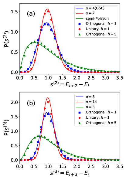
Figure 2: Distribution of next-nearest level spacings $P(s^{(2)})$ in (a) and next-next-nearest level spacings $P(s^{(3)})$ in (b), where $\alpha$ and $n$ are the index in Eq. (16) and Eq. (20) respectively.

As expected, the fittings are quite accurate for both GOE and GUE as well as Poisson ensemble. In fact, the fittings for higher order spacings in the Poisson ensemble are better than that for nearest spacing in Fig. 1(b). This is because in MBL phase the overlap between levels decays exponentially with their distance, hence the fitting for higher order level spacings is less affected by finite size effect.

For another example we consider the non-trivial zeros of the Riemann zeta functionzeta

$$\zeta\left(z\right)=\sum_{n=1}^{\infty}\frac{1}{n^{z}}\text{,}$$ (21)

it was established that statistical properties of non-trivial Riemann zeros $\left\{\gamma_{i}\right\}$ are well described by the GUE distributionZeta . Therefore, we expect the gaps $\left\{s_{i}^{(n)}=\gamma_{i+n}-\gamma_{i}\right\}$ follows the same distribution as those in GUE. The numerical results for $n=1,2,3$ are presented in Fig. 3, as can be seen, the fittings are perfect.

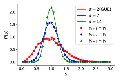
Figure 3: The distribution of $n$-th order spacings of the non-trivial zeros $\{\gamma_{i}\}$ of Riemann zeta function, where $\alpha$ is the index in generalized Wigner-Dyson distribution in Eq. (16). The data comes from $10^{4}$ levels starting from the $10^{22}$th zero, taken from Ref. [Odlyzko, ].

IV Higher Order Gap Ratios

As mentioned in Sec. I, besides the level spacings, another quantity is also widely used in the study of random matrices, namely the ratio between adjacent gaps $\left\{r_{i}=s_{i+1}/s_{i}\right\}$, which is independent of local DOS. The distribution of nearest gap ratios $P\left(\nu,r\right)$ is given in Ref. [Atas, ], whose result is

$$P\left(\nu,r\right)=\frac{1}{Z_{\nu}}\frac{\left(r+r^{2}\right)^{\nu}}{\left(1+r+r^{2}\right)^{1+3\nu/2}}$$ (22)

where $\nu=1,2,4$ for GOE,GUE,GSE, and $Z_{\nu}$ is the normalization factor determined by requiring $\int_{0}^{\infty}P\left(\nu,r\right)dr=1$.

This gap ratio can also be generalized to higher order, but in different ways, i.e. the “overlapping” Atas ; Atas2 and “non-overlapping” Tekur ; Chavda way. In the former case we are dealing with

$$\widetilde{r}_{i}^{\left(n\right)}=\frac{E_{i+n}-E_{i}}{E_{i+n-1}-E_{i-1}}=\frac{s_{i+n}+s_{i+n-1}+...+s_{i+1}}{s_{i+n-1}+s_{i+n-2}+...+s_{i}}\text{,}$$ (23)

which is named “overlaping” ratio since there is shared spacings between the numerator and denominator. While the “non-overlapping” ratio is defined as

$$r_{i}^{\left(n\right)}=\frac{E_{i+2n}-E_{i+n}}{E_{i+n}-E_{i}}=\frac{s_{i+2n}+s_{i+2n-1}+...+s_{i+n+1}}{s_{i+n}+s_{i+n-1}+...+s_{i}}\text{.}$$ (24)

Both these two generalizations reduce to the nearest gap ratio when $n=1$, but they are quite different when studying their distributions using Wigner surmise: for overlapping ratio $\widetilde{r}_{i}^{\left(n\right)}$, the smallest matrix dimension is $\left(n+2\right)\times\left(n+2\right)$; while it is $\left(1+2n\right)\times\left(1+2n\right)$ for non-overlapping ratio. Naively, we can expect the distribution for $\widetilde{r}^{\left(n\right)}$ is more involved due to the overlapping spacings. Indeed, the $n=2$ case for $P\left(\widetilde{r}^{\left(n\right)}\right)$ has been worked out in Ref. [Atas2, ] and the result is very complicated. Instead, for the non-overlapping ratio, Ref. [Tekur, ] provides compelling numerical evidence for its distribution to follow

$$P\left(\nu,r^{\left(n\right)}\right) = P\left(\nu^{\prime},r\right)\text{, }$$ (25)

$$\nu^{\prime} = \frac{n\left(n+1\right)}{2}\nu+n-1\text{.}$$ (26)

Surprisingly, the rescaling relation Eq. (26) coincides with that for higher order level spacing in Eq. (17). We have also confirmed this formula by numerical simulations in our spin model Eq. (7), and the results for $n=2$ in GOE ($\nu=1$) case is presented in Fig. 4, where we also draw the distribution of overlapping ratio $\widetilde{r}^{\left(2\right)}$ for comparison. As can be seen, they differ dramatically, and the fitting for non-overlapping ratio is quite accurate. This result strongly suggest the non-overlapping ratio is more universal than the overlapping ratio, and its distribution $P\left(r^{\left(n\right)}\right)$ is homogeneously related with that for the $n-$th order level spacing, at least in the sense of Wigner surmise, for which we provide a heuristic explanation as follows.

For a given energy spectrum $\left\{E_{i}\right\}$ from a Gaussian ensemble with index $\nu$, we can make up a new spectrum $\left\{E_{i}^{{}^{\prime}}\right\}$ by picking one level from every $n$ levels in $\left\{E_{i}\right\}$, then the $n$-th order level spacing $s^{\left(n\right)}$ in $\left\{E_{i}\right\}$ becomes the nearest level spacing in $\left\{E_{i}^{{}^{\prime}}\right\}$, and the $n$-th order non-overlapping ratio in $\left\{E_{i}\right\}$ becomes the nearest gap ratio in $\left\{E_{i}^{{}^{\prime}}\right\}$. Since we have analytically proven the rescaling relation in Eq. (17), we conjecture the probability density for $\left\{E_{i}^{{}^{\prime}}\right\}$ (to leading order) bear the same form as $\left\{E_{i}\right\}$ in Eq. (1) with the rescaled parameter $\alpha$ in Eq. (17). Therefore, the higher order non-overlapping gap ratios also follow the same rescaling as expressed in Eq. (25) and Eq. (26). For this point of view, numerical evidences are provided in a recent work of the authorRao20 .

Figure 4: The distribution of second-order gap ratio in the orthogonal model, where red and blue dots correspond to overlapping and non-overlapping ratios respectively, the latter fits perfectly with the formula in Eq. (25) with $\nu^{\prime}=4$. Note the data is taken from the whole energy spectrum without unfolding.

V Conclusion and Discussion

We have analytically studied the distribution of higher order level spacings $\left\{s_{i}^{\left(n\right)}=E_{i+n}-E_{i}\right\}$ which describes the level correlations on long range. It is shown $s^{\left(n\right)}$ in the Gaussian ensemble with index $\nu$ follows a generalized Wigner-Dyson distribution with index $\alpha=\nu C_{n+1}^{2}+n-1$, where $\nu=1,2,4$ for GOE,GUE,GSE respectively. This results in a large number of coincident relations for distributions of level spacings of different orders in different ensembles. While $s^{\left(n\right)}$ in Poisson ensemble follows a generalized semi-Poisson distribution with index $n$. Our derivation is rigorous based on a Wigner-like surmise, and the results have been confirmed by numerical simulations from random spin system and non-trivial zeros of Riemann zeta function.

We also discussed the higher order generalization of gap ratios, which come in two different ways – the “overlapping” and “ non-overlapping” way – and point out their difference in studying their distributions using Wigner-like surmise. Notably, the distribution for the non-overlapping gap ratio has been studied numerically in Ref. [Tekur, ], in which the authors find a scaling relation Eq. (26) that is identical to the one we find analytically for higher order level spacings. This strongly indicates the distribution of higher order spacing and non-overlapping gap ratio is correlated in a homogeneous way, for which we provided a heuristic explanation.

It’s noted the higher-order level spacings have played an important role in the study of the spacing distribution in a spectrum with missing levelsBohigas , where the second order level spacing distribution in GOE is derived by a method different from this work. Our derivations for $P\left(s^{\left(n\right)}\right)$ in Guassian ensembles are purely mathematical that work for arbitrary positive values of $\nu$, although the $\nu=1,2,4$ for GOE,GUE,GSE are of most physical interest. Therefore, it is possible for our results to find applications in models that goes beyond the three standard Gaussian ensembles. For example, the $\nu=3$ behavior for level spacing has been found in a 2D lattice with non-Hermitian disorderTzortzakakis .

It is also interesting to note the distribution of next-nearest level spacing in Poisson class is semi-Poisson $P_{2}\left(s\right)\propto s\exp\left(-2s\right)$, which is suggested to be the distribution for nearest level spacing at the thermal-MBL transition point in orthogonal model Serbyn . This indicates – to leading order – the universality property of this transition point is more affected by the MBL phase than the thermal phase, a fact already noticed by previous studiesHuse2 ; Serbyn . This observation thus motivates a natural question: how will the thermal phase affect the universality of the MBL transition point? To answer this question, a comparison between the GOE-Poisson and GUE-Poisson transition points is suggested, which is left for a future study.

Last but not least, in this paper the distribution of higher order level spacing is derived only in $\left(n+1\right)\times\left(n+1\right)$ matrix, its exact value in large matrix as well as the difference between them can in principle be estimated using the method in Ref. [Atas, ], this is also left for a future study.

References

- (1) C. E. Porter, Statistical Theories of Spectra: Fluctuations (Academic Press, New York), 1965.
- (2) T. A. Brody et al., Rev. Mod. 53, 385 (1981).
- (3) T. Guhr, A. Muller-Groeling, H. A. Weidenmuller, Phys. Rep. 299, 189 (1998).
- (4) M. L. Mehta, Random Matrix Theory, Springer, New York (1990).
- (5) F. Haake, Quantum Signatures of Chaos (Springer 2001).
- (6) E. P. Wigner, in Conference on Neutron Physics by Timeof-Flight (Oak Ridge National Laboratory Report No. 2309, 1957) p. 59.
- (7) V. Oganesyan and D. A. Huse, Phys. Rev. B 75, 155111 (2007).
- (8) Y. Y. Atas, E. Bogomolny, O. Giraud, and G. Roux, Phys. Rev. Lett. 110, 084101 (2013).
- (9) V. Oganesyan, A. Pal, D. A. Huse, Phys. Rev. B 80, 115104 (2009).
- (10) A. Pal, D. A. Huse, Phys. Rev. B 82, 174411 (2010).
- (11) S. Iyer, V. Oganesyan, G. Refael, D. A. Huse, Phys. Rev. B 87, 134202 (2013).
- (12) X. Li, S. Ganeshan, J. H. Pixley, and S. Das Sarma, Phy. Rev. Lett. 115, 186601 (2015).
- (13) Y. Bar Lev, G. Cohen, and D. R. Reichmman, Phys. Rev. Lett. 114, 100601 (2015).
- (14) K. Agarwal, S. Gopalakrishnan, M. Knap, M. Mueller, and E. Demler, Phys. Rev. Lett. 114 160401 (2015).
- (15) David J. Luitz, Nicolas Laflorencie, and Fabien Alet, Phys. Rev. B 91, 081103(R) (2015).
- (16) Y. Avishai, J. Richert, and R. Berkovits, Phys. Rev. B 66, 052416 (2002).
- (17) N. Regnault and R. Nandkishore, Phys. Rev. B 93, 104203 (2016).
- (18) S. D. Geraedts, R. Nandkishore, and N. Regnault, Phys. Rev. B 93, 174202 (2016).
- (19) P. Shukla, New Journal of Physics 18, 021004 (2016).
- (20) M. Serbyn and J. E. Moore, Phys. Rev. B 93, 041424(R) (2016).
- (21) E. B. Bogomolny, U. Gerland and C. Schmit, Eur. Phys. J. B 19, 121 (2001).
- (22) P. Sierant and J. Zakrzewski, Phys. Rev. B 99, 104205 (2019).
- (23) W. Buijsman, V. Cheianov and V. Gritsev, Phys. Rev. Lett. 122, 180601 (2019).
- (24) P. Sierant and J. Zakrzewski, Phys. Rev. B 101, 104201 (2020).
- (25) J. M. G. Gomez, R. A. Molina, A. Relano, and J. Retamosa, Phys. Rev. E 66, 036209 (2002).
- (26) Y. Y. Atas, E. Bogomolny, O. Giraud, P. Vivo, and E. Vivo, J. Phys. A: Math. Theor. 46, 355204 (2013).
- (27) S. H. Tekur, S. Kumar and M. S. Santhanam, Phys. Rev. E, 97, 062212 (2018).
- (28) S. H. Tekur, U. T. Bhosale, and M. S. Santhanam, Phys. Rev. B 98, 104305 (2018).
- (29) P. Rao, M. Vyas, and N. D. Chavda, arXiv:1912.05664v1.
- (30) A. Y. Abul-Magd and M. H. Simbel, Phys. Rev. E 60, 5371 (1999).
- (31) M. M. Duras and K. Sokalski, Phys. Rev. E 54, 3142 (1996).
- (32) R. Kausar, W.-J. Rao, and X. Wan, J. Phys.: Condens. Matter 32, 415605 (2020).
- (33) W.-J. Rao, J. Phys.:Condens. Matter 30, 395902 (2018).
- (34) M. L. Mehta and F. J. Dyson, Journal of Mathematical Physics, 4 (1963).
- (35) E. B. Bogomolny, U. Gerland and C. Schmit, Phys. Rev. E 59, R1315(R) 1999.
- (36) Definition of the Riemann function given in Eq. (21) is valid only for Re. To overcome this problem, see, e.g., H. M. Edwards, ”Riemann’s Zeta Function”, Chap.1.4.
- (37) H. L. Montgomery, Proc. Symp. Pure Math. 24, 181 (1973); E. B. Bogomolny and J. P. Keating, Nonlinearity 8, 1115 (1995); ibid Nonlinearity 9, 911 (1995); Z. Rudnick and P. Sarnak, Duke Math. J. 81, 269 (1996); J. P. Keating and N. C. Snaith, Comm. Math. Phys. 214, 57 (2000).
- (38) A. Odlyzko, www.dtc.umn.edu/odlyzko/zeta_tables/index.html.
- (39) W.-J. Rao and M. N. Chen, arXiv:2006.07774.
- (40) O. Bohigas and M. P. Pato, Phys. Lett. B 595, 171-176 (2004).
- (41) A. F. Tzortzakakis, K. G. Makris, and E. N. Economou, Phys. Rev. B 101, 014202 (2020).