Generalizing optimal Bell inequalities

Abstract

Bell inequalities are central tools for studying nonlocal correlations and their applications in quantum information processing. Identifying inequalities for many particles or measurements is, however, difficult due to the computational complexity of characterizing the set of local correlations. We develop a method to characterize Bell inequalities under constraints, which may be given by symmetry or other linear conditions. This allows to search systematically for generalizations of given Bell inequalities to more parties. As an example, we find all possible generalizations of the two-particle inequality by Froissart [Il Nuovo Cimento B64, 241 (1981)], also known as I3322 inequality, to three particles. For the simplest of these inequalities, we study their quantum mechanical properties and demonstrate that they are relevant, in the sense that they detect nonlocality of quantum states, for which all two-setting inequalities fail to do so.

Introduction.— Bell nonlocality describes the fact that quantum mechanical correlations are stronger than the ones predicted by local hidden variable (LHV) models Brunner et al. (2014); Scarani (2019). This manifests itself in the violation of Bell inequalities, which have been observed experimentally Shalm et al. (2015); Hensen et al. (2015); Giustina et al. (2015); Rosenfeld et al. (2017). Besides ruling out hidden variable models, however, Bell inequalities are also essential for studying information theory with distributed parties Buhrman et al. (2010). In fact, various Bell inequalities found interesting applications and led to surprising insights to quantum information processing. Examples are the connection between Bell inequalities and communication complexity Brukner et al. (2004); Tavakoli et al. (2020), multi-player games which demonstrate the difference between quantum mechanics and non-signaling theories Almeida et al. (2010), Bell inequalities that are useful for multiparty conference key agreement Holz et al. (2020) and the emerging field of self-testing, where Bell inequalities play also a central role, see Šupić and Bowles (2020) for a review. Therefore, although LHV models are considered to be experimentally refuted, it is desirable to identify Bell inequalities with interesting properties.

Characterizing all the Bell inequalities is, however, not straight forward. For a given number of parties, if one fixes the number of measurement settings and the outcomes per measurement, the set of all probabilities coming from LHV models forms a high-dimensional polytope and the Bell inequalities correspond to the facets of this polytope Peres (1999); Pitowsky (1991). The extremal points of this polytope are easy to characterize, but it is computationally very demanding to find all the facets from the extremal points Pitowsky (1991). The rising complexity can be directly illustrated with an example. If one considers two parties with two measurements ($A_{1},A_{2}$ and $B_{1},B_{2}$) and two outcomes ($\pm 1$), it is well known that there is, up to relabelings and permutations, only one optimal Bell inequality Fine (1982), known as the Clauser-Horne-Shimony-Holt (CHSH) inequality Clauser et al. (1969, 1970). It reads

$$\langle{A_{1}B_{1}}\rangle+\langle{A_{1}B_{2}}\rangle+\langle{A_{2}B_{1}}\rangle-\langle{A_{2}B_{2}}\rangle\leq 2.$$ (1)

Some generalizations of it, using more particles but still two measurements per site, have been found Werner and Wolf (2001); Żukowski and Brukner (2002); Śliwa (2003).

If one considers two particles with three measurements, the analysis becomes already considerably harder. It was shown that there is only one additional Bell inequality. This was first identified by Froissart Froissart (1981), and later independently by Śliwa Śliwa (2003) and Collins and Gisin Collins and Gisin (2004) . It reads

$$\langle{A_{1}}\rangle -\langle{A_{2}}\rangle+\langle{B_{1}}\rangle-\langle{B_{2}}\rangle-\langle{(A_{1}-A_{2})(B_{1}-B_{2})}\rangle$$

$$+\langle{(A_{1}+A_{2})B_{3}}\rangle+\langle{A_{3}(B_{1}+B_{2})}\rangle\leq 4.$$ (2)

This inequality, henceforth called I3322 inequality, has several interesting properties: It detects the nonlocality of some two-qubit states which are not detected by the CHSH inequality Collins and Gisin (2004), and, for higher dimensions, the maximal violation of it is not attained at maximally entangled states Vidick and Wehner (2011). In general, the violation of I3322 is conjectured to increase with the dimension of the underlying quantum system Pál and Vértesi (2010) and, since the maximal violation can definitely not occur in small-dimensional systems Moroder et al. (2013); Navascués and Vértesi (2015), I3322 can be used for the device-independent characterization of the dimension. Clearly, it is highly desirable to find generalizations of I3322 to three or more particles, but the exponentially increasing complexity of a brute force approach has prevented this so far.

In this paper, we present a systematic approach to find all Bell inequalities obeying some linear constraints. This constraint may be given by a desired symmetry or it may be formulated such that the Bell inequality should reduce to some fixed expression in special cases. With our method, we find all 3050 generalizations of the I3322 inequality to three particles, and then we characterize the physical properties of the simplest ones of the new inequalities. Our method generalizes previous methods to characterize Bell inequalities constrained by symmetry Bancal et al. (2010) in a constructive manner, as it can be used to systematically find all generalizations of a known inequality.

Bell inequalities and convex geometry.— A Bell scenario is characterized by the number of parties $N$, the number of measurement settings per party $I$ and the number of outcomes $O$ per measurement. For a given scenario, the behavior of a physical system can be encoded in a vector that contains all the probabilities for the outcomes of all possible joint measurements on the subsystems. Concretely, the correlations of a system are encoded in the vector that contains all probabilities $p(o_{1},...,o_{N}|i_{1},...,i_{N})$, where $o_{k}\in\{1,...,O\}$ denotes the outcomes for the settings $i_{k}\in\{1,...,I\}$. In the simple case of dichotomic measurements (with outcomes $\pm 1$), the correlations can alternatively be characterized as the collection of the expectation values of joint measurements. This is also how the CHSH- and I3322 inequality were formulated above.

We call systems that can be described by an LHV model classical. Such systems can be characterized in the following way. First, one considers the finite set of probability vectors with local deterministic assignments, where each probability is $0$ or $1$ and the results of joint measurements on different systems are uncorrelated. Then, one considers all probabilistic mixtures of these vertices, i.e. the convex hull. The resulting set of all classical behaviors forms a convex polytope, the so-called local polytope. As any polytope, the local polytope is uniquely represented by its vertices as extremal points, but one can alternatively describe it by linear inequalities.

In fact, a Bell inequality is nothing but a linear inequality in the space of the probabilities, which holds on the local polytope. So, it defines two half-spaces in the space of correlations, such that one half-space contains the local polytope and the other half-space is detected as nonlocal. Clearly, the most efficient characterization of the local polytope is the minimal set of half-spaces whose intersection equals the polytope. These correspond to the optimal Bell inequalities and are characterized by the facets of the polytope . It is easy to check whether a given linear inequality corresponds to a facet of the local polytope, as one just has to find enough vertices that saturate it. The conversion from the vertex description to the half-space description of the local polytope is, however, difficult in practice and is known to be hard for the general case Pitowsky (1991).

The main method.— We consider the situation where a convex polytope $P$ in vertex representation is given and one aims to find all facets of $P$ that satisfy some linear conditions. The naive way of solving this problem is to first find all facets of $P$ and filter out all those inequalities that do not meet the conditions in a second step. In practice, however, already the first step is often to complex to be solved. Our method to solve this problem works for the case that the conditions are affine equality constraints on the coefficients of the facet defining inequality.

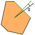
(a)

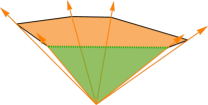
(b)

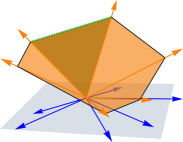
(c)

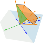
(d)

Figure 1: Visualization of the method to find Bell inequalities that obey some constraints. (a) We aim to find facets of the two-dimensional polytope $P$ with a normal vector $\bm{b}_{P}$ that has a fixed scalar product with some vector $\bm{g}$. The facet and the normal vector that fulfill this constraint drawn in green. (b) We embed the polytope $P$ in a plane in three-dimensional space. The coordinates of the vertices of $P$ define rays (orange arrows) that define the cone $C$. The polytope $P$ is then a section of the cone $C$ and each of its facets relates to a facet of $C$ (green) in a unique way. (c) The initial constraint on the facet of $P$ can be translated. A facet of $P$ fulfills the constraint if and only if the corresponding facet of $C$ has a normal vector $\bm{b}_{C}$ that obeys a linear constraint $G\bm{b}_{C}=0$, which means that it has to lie in a plane (light-grey). Then, we project the rays of $C$ (orange) into that plane (blue arrows) to define a cone $\widetilde{C}$ as generated by the projected rays. By construction, facets of $C$ which obey the constraint are also facets of $\widetilde{C}$. (d) Finally we find the facets of $\widetilde{C}$ and check which ones correspond to facets of $C$. From the facets of $C$ that meet the conditions we can then compute the corresponding facets of $P$. In our example, $\widetilde{C}$ is a half plane (light-blue) and has only one facet, with the normal vector in green. It is also the normal vector of a facet of $C$ (green). Note that in the example $\widetilde{C}$ is already generated by three rays and the other three rays are redundant.

In the following, we describe the main ideas of the different steps, details are given in Appendix A . We start with the original $D$-dimensional polytope $P$ and the constraints, which can be written in the form that the normal vector $\bm{b}_{P}$ on the facet has a fixed scalar product with some vector $\bm{g}$, see Fig. 1(a). Then, we construct a cone $C$ in $D+1$-dimensional space that maintains a one-to-one correspondence to the polytope, since the polytope can be seen as a cut of the cone, see Fig. 1(b). Notably, there is a one-to-one correspondence between the facets of the cone and those of the polytope, and a normal vector $\bm{b}_{P}$ of a polytope facet translates to a normal vector $\bm{b}_{C}$ of a cone facet. Also, this construction allows to write the constraints in a linear form as $G\bm{b}_{C}=0$, see Fig. 1(c).

The key observation is that in this situation we can define a new cone $\widetilde{C}$, such that if $\bm{b}_{C}$ is a facet normal vector of $C$ that obeys the constraints, then $\bm{b}_{C}$ is also a facet normal vector of $\widetilde{C}$. This is done by projecting the rays of $C$ down to the subspace of vectors obeying $G\bm{v}=0$, see Fig. 1(c). The advantage is that $\widetilde{C}$ lies in a significantly lower-dimensional space. Additionally, $\widetilde{C}$ has typically much less rays than $C$. That makes it easier to find all the facets of $\widetilde{C}$, compared with $C$. Having obtained all the facets of $\widetilde{C}$, it remains to check whether they are facets of $C$. If this is the case, they automatically obey the constraints, see Fig. 1(d).

Tripartite generalizations of I3322.— Let us apply our method to the scenario where three parties perform three dichotomic measurements. This scenario is already too complex to find all facets of the local polytope: The three-partite scenario with two dichotomic measurements per party has 64 vertices in 26 dimensions and 53856 facets already Śliwa (2003). Concerning the scenario we are interested in, we only know that the local polytope has 512 vertices in a 63-dimensional space. Bancal and coworkers have investigated this scenario while restricting themselves to symmetric, full-body correlation inequalities and they found 20 facet defining Bell inequalities of this type Bancal et al. (2010). However, due the fact that marginal correlations prove to be vital for the I3322 inequality, the restriction to Bell inequalities without them seems to be ad-hoc.

The notion of generalizing a bipartite Bell inequality to more parties is best introduced by example. Consider the Mermin inequality for three parties,

$$\langle{A_{1}B_{1}C_{2}}\rangle+\langle{A_{1}B_{2}C_{1}}\rangle+\langle{A_{2}B_{1}C_{1}}\rangle-\langle{A_{2}B_{2}C_{2}}\rangle\leq 2.$$ (3)

If one assigns the fixed values $C_{1}=C_{2}=1$ (or some other values) on the third party, then this inequality reduces to the CHSH inequality in Eq. (1) (or a variant thereof). In this sense, one may view the Mermin inequality as a generalization of the CHSH inequality.

The formal definition of a generalization of the I3322 inequality is as follows. First, since all measurements are dichotomic, we write all Bell inequalities in terms of expectation values of observables. Observables that refer to measurements of party $A$ ($B$, $C$) are denoted as $A_{i}$ ($B_{j}$, $C_{k}$) and we define $A_{0},B_{0},C_{0}$ to be trivial measurements on the respective parties that always yield a measurement result $+1$. This conveniently allows to treat marginal terms such as $\langle{A_{1}}\rangle=\langle{A_{1}B_{0}C_{0}}\rangle$ and constant terms such as $1=\langle{A_{0}B_{0}C_{0}}\rangle$ on the same footing. In this notation, any Bell inequality can be written as $S=\sum_{i,j,k}b_{ijk}\langle A_{i}B_{j}C_{k}\rangle\geq 0.$

We call a three-partite Bell inequality a generalization of the I3322 inequality if the following three conditions hold: (a) The inequality is symmetric under exchange of the parties, each of which can perform three different non-trivial dichotomic measurements, (b) The inequality corresponds to a facet of the local polytope, and (c) There is an assignment $C_{k}\to\xi_{k}\in\{\pm 1\}$ for the observables on the third party, such that the remaining inequality $\sum_{i,j,k}b_{ijk}\xi_{k}\langle A_{i}B_{j}\rangle\geq 0$ is the I3322 inequality as in Eq. (2). The analogous condition with the same $\xi_{k}$ holds for any other reduction to two parties. Note that this approach is different from the notion of lifting Bell inequalities to more parties Pironio (2005), where, e.g., a two-party Bell inequality is applied to the conditional probabilities of a three-party system.

The properties (a) and (b) are natural requirements, because both are characteristic features of the I3322 inequality. Besides its mathematical motivation, condition (c) has physical consequences. It implies that the new inequality detects nonlocality in a three-partite state $\varrho_{ABC}$ every time the I3322 inequality detects it in the reduced state $\varrho_{AB}.$ Indeed, if condition (c) holds, one can just choose trivial measurements for the $C_{k}$ that yield outcomes $\xi_{k}\in\{\pm 1\}$ independently of the state. Then the generalization of I3322 also detects the nonlocality.

For our method, we also note that condition (c) can be reformulated as follows: An inequality like $\sum_{i,j,k}b_{ijk}\xi_{k}\langle A_{i}B_{j}\rangle\geq 0$ is the I3322 inequality, if and only if equality holds for the set of vertices for which also equality holds in I3322. These bipartite vertices may be lifted to three-partite vertices by adding the variable $\xi_{k}$, then any generalization of the I3322 inequality has to be saturated by these lifted vertices. The critical reader may ask at this point why we are only considering the special form of I3322 as in Eq. (2), and not equivalent forms arising from a relabeling of the observables or a sign flip. First, since we defined generalizations of I3322 to be symmetric, we only have to take symmetric versions of I3322 into account. Further, as one can easily check, all symmetric versions of I3322 can be transformed into each other just by outcome relabelings on both parties. Consequently, it suffices to only consider one symmetric version of I3322.

We can now find all generalizations of I3322 in four steps: First, we find all vertices of the local polytope of two parties which saturate I3322. Second, we choose deterministic outcomes $\xi_{k}$ on $C$ and determine the corresponding vertices in the local polytope of three parties. In the third step, we compose the matrix $G$ for the condition $G\bm{b}_{C}=0$. This matrix contains each symmetry condition and each vertex from step 2 as a row. Finally, we employ our method as described above to find all facet defining inequalities that meet the criteria. We then repeat steps two to four until all possible choices for deterministic outcomes $\xi_{k}$ are exhausted. In our case of three dichotomic measurements, there are eight possibilities. In this way, we find all symmetric, facet-defining generalizations of I3322, $3050$ inequalities in total. Details of the implementation are given in Appendix B and the complete list is given in the supplemental material.

Properties of the generalizations of I3322.— Let us now examine the three simplest ones among the generalized I3322 inequalities in some detail. For convenience, we introduce a short-hand notation for symmetric Bell inequalities. We define symmetric correlations as $(ijk)=\sum_{\pi\in\Pi}A_{\pi(i)}B_{\pi(j)}C_{\pi(k)}$, where $\Pi$ denotes the set of all permutations of the indices $ijk$ that give different terms. Note that in this notation $(112)=A_{1}B_{1}C_{2}+A_{1}B_{2}C_{1}+A_{2}B_{1}C_{1}$, so permutations leading to the same term are not counted multiple times. Further, as noted before, settings labeled with index zero refer to trivial measurements that always yield the result $1$. Using this notation, the I3322 inequality in Eq. (2) can be written as

$$(01)-(02)-(11)-(22)+(12)+(13)+(23)\leq 4.$$ (4)

The three generalizations of I3322 that involve the least number of symmetric correlations are given by:

$$F_{1} =8+(110)-(210)+(211)+(220)$$

$$+(222)-2(331)-2(332)\geq 0,$$ (5)

$$F_{2} =9+(110)+2(220)-2(221)-(300)$$

$$-(310)+(311)-2(322)\geq 0,$$ (6)

$$F_{3} =9-(210)+(211)+(220)+3(222)$$

$$-(300)-(310)+(311)-2(322)\geq 0.$$ (7)

Let us start our analysis with the possible violations in quantum mechanics. It has recently been shown that all inequalities that exclusively utilize full correlations are violated in quantum mechanics Escolà et al. (2020), however, our inequalities also contain marginal terms.

A way to obtain bounds on possible quantum values of Bell inequalities is given by the hierarchy of Navascués, Pironio and Acín (NPA) Navascués et al. (2007, 2008); Wittek (2015). For the inequality $F_{1}$, this shows that in quantum mechanics $F_{1}\geq-8$ holds. The minimal value $F_{1}=-8$ can indeed be reached, namely by a three-qubit GHZ state $|GHZ_{3}\rangle=(|000\rangle+|111\rangle)/\sqrt{2}$ and measurements $A_{1}=A_{2}=\sigma_{x}$, $A_{3}=\sigma_{y}$, $B_{1}=B_{2}=-\sigma_{y}$, $B_{3}=\sigma_{x}$ and $C_{i}=B_{i}$. In fact, $F_{1}$ reduces to the Mermin inequality in Eq. (3) if the first two measurement settings on each party are chosen equal.

Concerning $F_{2}$, a numerical optimization suggests that one optimal choice of settings is given by $A_{1}=-A_{3}=\sigma_{z}$, $A_{2}=-\sigma_{x}$, $B_{1}=-B_{3}=-\sigma_{z}$, $B_{2}=-\sigma_{x}$, and $C_{i}=B_{i}$. This leads to a quantum mechanical violation of $F_{2}=4(1-\sqrt{7})\approx-6.58301$ for the three-qubit state

$$|\psi_{2}\rangle=a|W_{3}\rangle+b|111\rangle,$$ (8)

with $|W_{3}\rangle=(|001\rangle+|010\rangle+|100\rangle)/\sqrt{3}$ being the three-qubit W state and $a=\sqrt{19+2\sqrt{7}}/\sqrt{74}\approx 0.57294$ and $b=\sqrt{55-2\sqrt{7}}/\sqrt{74}\approx 0.81960.$ The violation attained by this state coincides up to numerical precision with the lower bound on $F_{2}$ for quantum states from the NPA hierarchy. It is interesting that $F_{2}$ is maximally violated by a state that does not belong to the frequently studied three-qubit states (such as the states considered in Bruß et al. (1998); Hein et al. (2004); Gühne et al. (2014)). In this way, the Bell inequality $F_{2}$ may open an avenue for new methods of self-testing quantum states Šupić and Bowles (2020).

For the inequality $F_{3}$ the third level of the NPA hierarchy bounds the quantum mechanical values by $F_{3}\geq-4.63097.$ Within numerical precision, this can be attained using the three-qubit state

$$|\psi_{3}\rangle=\cos(\varphi)|W_{3}\rangle+\sin(\varphi)|GHZ_{3}\rangle$$ (9)

with $\varphi=4.0^{\circ}$. The required measurement settings (for $i=1,2,3$) are $A_{i}=\cos(\alpha_{i})\sigma_{z}+\sin(\alpha_{i})\sigma_{x}$ and $B_{i}=C_{i}=\cos(\alpha_{i})\sigma_{z}-\sin(\alpha_{i})\sigma_{x}$, where $\alpha_{1}=141.6^{\circ},\alpha_{2}=22.6^{\circ},\alpha_{3}=101.6^{\circ}.$ Again, we find a non-standard three-qubit state leading to the maximal violation of the Bell inequality. The state $|\psi_{3}\rangle$ is close to a three-qubit W state but the difference is significant, as for the W state one can only reach a violation of $F_{3}=-4.59569$.

Now we clarify whether the new three-setting inequalities are indeed relevant, that is, whether they detect the nonlocality of some quantum states, where all two-setting inequalities fail to do so. This question can be answered positively for all three inequalities; moreover, all the $F_{i}$ detect also entanglement that is not detected by the I3322 inequality in the reduced states. To show this, we provide a three-qubit state $\varrho_{ABC}$ with separable two-body marginals that has a symmetric extension for each $F_{i}$, such that the respective Bell inequality $F_{i}$ is violated. A symmetric extension of $\varrho_{ABC}$ is a five-qubit state $H_{ABB^{\prime}CC^{\prime}}$ that is symmetric under exchange of the parties $B$, $B^{\prime}$ (and $C$, $C^{\prime}$) such that $\varrho_{ABC}=\text{Tr}_{B^{\prime}C^{\prime}}(H_{ABB^{\prime}CC^{\prime}})$. A state that has a such a symmetric extension cannot violate any Bell inequality with with an arbitrary number of settings for Alice and two settings for Bob and Charlie Terhal et al. (2003), see also Appendix C. Note that here the number of outcomes for each setting is unrestricted. Thus this is a stronger statement than proving that the known inequalities for two settings and two outcomes Werner and Wolf (2001); Żukowski and Brukner (2002); Śliwa (2003) are not violated.

We find the desired state $\varrho_{ABC}$ using a seesaw algorithm that alternates between optimizing the measurement settings (for the violation of the $F_{i}$) and the state (under some constraints). If measurement settings for all parties are fixed, finding a state with a symmetric extension that maximally violates a given $F_{i}$ is a semidefinite program. On the other hand, given a state and measurement settings for two parties, finding the optimal settings for the third party is also a semidefinite program. Details and examples are discussed in Appendix C.

Conclusion.— We presented a method to find all Bell inequalities for a given Bell scenario under some constraints. Our method does not require to characterize the local polytope completely, instead, all candidates for the desired Bell inequalities can be found in a low-dimensional projection of the cone corresponding to the polytope. Using our method, we characterized all generalizations of the I3322 inequality to three particles. It turned out that already the simplest ones of these generalizations have interesting properties, making an experimental implementation of them desirable.

Our method can be used for many other purposes, where convex polytopes play a role. First, one may consider other Bell scenarios, e.g., cases where not all parties have the same number of measurements. In addition, one can generalize also contextuality inequalities Budroni et al. (2020) or recently discussed inequalities for testing certain views of quantum mechanics Bong et al. (2020). Moreover, it could be interesting to extend our approach beyond the scenario of linear optimization: While the local polytope in Bell scenarios can be characterized by the optimization method of linear programming, other forms of quantum correlations, such as quantum steering, are naturally described in terms of convex optimization and semidefinite programs Cavalcanti and Skrzypczyk (2017); Uola et al. (2020). Thus, a generalization of our methods to this type of problems could give more insight into various problems in information processing.

Acknowledgements.— We thank Jędrzej Kaniewski, Miguel Navascués, Chau Nguyen and Denis Rosset for fruitful discussions. This work has been supported by the Deutsche Forschungsgemeinschaft (DFG, German Research Foundation - 447948357) and the ERC (Consolidator Grant 683107/TempoQ). FB acknowledges support from the House of Young Talents of the University of Siegen.

I Appendix A: Details of the method

I.1 Some terminology for convex polyhedra

We follow the standard terminology as introduced in the textbook by Ziegler Ziegler (1995) and refer to convex polyhedra simply as polyhedra, since we are only concerned with the convex variety. The two arguably most fundamental concepts in this context are conic combinations and convex combinations. Conic combinations are linear combinations with positive coefficients. Convex combinations are linear combinations with positive coefficients that sum up to one. Given a set $V$, the set that contains all conic (convex) combinations of the elements in $V$ is called the conic (convex) hull of $V$. Vice versa, the conic (convex) hull of $V$ is said to be generated by $V$ under conic (convex) combinations. If $V$ is finite, its convex hull is called finitely generated. These notions give rise to the two main objects that are studied, cones and polytopes, the first being finitely generated under conic combinations and the second being finitely generated under convex combinations. The elements of $V$ are called vertices in the case of polytopes. For cones, they are called rays.

The next useful definition is the Minkowski sum of two sets. Given two sets $A$ and $B$, this sum is defined as $A+B=\{a+b|a\in A,b\in B\}$. The Minkowski sum of a cone and a polytope is called polyhedron. The sets of rays and vertices that generate the polyhedron are called the V-representation of the polyhedron. That said, there is a second important represenation of polyhedra: the H-representation. Any polyhedron is the intersection of a finite number of half-spaces, defined by affine inequalities. The minimal set of half-spaces whose intersection is the polyhedron is its H-representation. With every of these half-spaces, we can associate the hyperplane that bounds it. The intersection between such a hyperplane and the polyhedron is called a facet of the polyhedron. If an inequality defines a half-space such that its bounding hyperplane contains a facet of a given polyhedron, this inequality is called facet-defining with respect to the polyhedron. If a polyhedron $P$ has dimension $D$, its facets are the $D-1$ dimensional polyhedra that together form the boundary of $P$. Intersections of facets are called faces. Hereby, an $n$-face is a face that has an (affine) dimension of $n$. Accordingly in the case of a $D$ dimensional polytope, $0$-faces are vertices, $1$-faces are edges and $(D-1)$-faces are facets.

I.2 Proof of the main statement

In the following, we describe a method to find all facet defining inequalities of a polytope of dimension $D$ that satisfy a set of linear equations. However, the possibility of these equations being inhomogenious makes that task cumbersome. Therefore, we embed the polytope in a $D+1$ dimensional space by prepending a coordinate to every vertex $\bm{v}_{i}$, that is we define

$$\bm{w}_{i}=\binom{1}{\bm{v}_{i}}.$$ (10)

We now consider the cone $C$ that is generated by the vectors $\bm{w}_{i}$. Note that we can retain the original polytope by intersecting the cone $C$ with the hyperplane defined by $x_{0}=1$. Because of its close relationship with the polytope, we call this cone the corresponding cone of the polytope. This relationship is not only reflected in the V-representation. There is also a one-to-one relation between the facet defining inequalities. Let

$$\bm{x}^{T}\bm{b}_{P}\geq-\beta$$ (11)

be a facet defining inequality of the polytope. Then,

$$(1\;\bm{x}^{T})\binom{\beta}{\bm{b}_{P}}\geq 0$$ (12)

is the corresponding facet defining inequality of the cone.

Now assume that we aim to find facets of the polytope that satisfy a given affine constraint

$$\bm{g}^{T}\bm{b}_{P}=\gamma.$$ (13)

Then we can reformulate this as an equivalent linear constraint on the facets of the cone by writing

$$(g_{0}\;\bm{g}^{T})\binom{\beta}{\bm{b}_{P}}=0$$ (14)

and choosing $g_{0}=-\frac{\gamma}{\beta}$. If we want to implement an affine constraint that also takes the bound of the inequality into account, one can accomplish this by adding another dimension, simply repeating the previous construction – this time for the cone. From the above discussion we conclude that finding facet defining inequalities of a polyhedron that satisfy affine equality constraints is equivalent to finding facet defining inequalities of the corresponding cone that satisfy linear equality constraints. We can hence pose the problem as follows: Given a cone $C$, find all of its facet normal vectors $\bm{b}_{C}$ that satisfy

$$G\bm{b}_{C}=0,$$ (15)

where $G$ is the matrix that captures all linear constraints. From Eq. (15) it follows that $\bm{b}_{C}$ is in the kernel of $G$. Let $\ker G=\text{span}(\{\bm{t}_{j}\}_{j=1}^{K})$. We define the matrix $T$ whose $K$ columns of length $D+1$ are made up by the vectors $\bm{t}_{j}$, so we have $T_{ij}=[\bm{t}_{j}]_{i}$. This allows us to decompose $\bm{b}_{C}$ in the basis of $\ker G$ as

$$\bm{b}_{C}=T\bm{b}_{\widetilde{C}},$$ (16)

where $\bm{b}_{\widetilde{C}}$ is a vector of dimension $K$. We will now find a cone $\widetilde{C}$ that has the same dimension as the kernel of $G$, such that any time $\bm{b}_{C}$ defines a facet of $C$ that satisfies $G\bm{b}_{C}=0$, $\bm{b}_{\widetilde{C}}$ defines a facet of $\widetilde{C}$. Since $\widetilde{C}$ is lower-dimensional compared to $C$ and has at most the same number of rays, it is easier to find the facets of $\widetilde{C}$ than of $C$. The effectivity and feasibility of the method therefore relies crucially on the dimension $K$ of the kernel of $G$. The higher-dimensional and difficult it is to find facets of $C$, the more linearly independent constraints are needed in order to make $\widetilde{C}$ low dimensional and simple enough so we can find its facets.

The following theorem establishes the construction of the cone $\widetilde{C}$.

Theorem 1.

Let $C=\text{cone}(\{\bm{w}_{i}\})$ be a cone and $\bm{b}_{C}$ a facet-normal vector of $C$ that satisfies $G\bm{b}_{C}=0$ for some matrix $G$. With $T$ and $\bm{b}_{\widetilde{C}}$ defined as above, we define the cone $\widetilde{C}=\text{cone}(\{\bm{\widetilde{w}_{i}}\})$ of dimension $K$ with $\bm{\widetilde{w}_{i}}^{T}=\bm{w_{i}}^{T}T$. Then $\bm{b}_{\widetilde{C}}$ defines a facet of $\widetilde{C}$.

Proof.

We prove the statement in three steps. (1) The inequality $\bm{\widetilde{w}_{i}}^{T}\bm{b}_{\widetilde{C}}\geq 0$ holds, since Eq. (16) together with the definition of the $\bm{\widetilde{w}_{i}}$ implies

$$\bm{\widetilde{w}_{i}}^{T}\bm{b}_{\widetilde{C}}=\bm{w_{i}}^{T}\bm{b}_{C}$$ (17)

and $\bm{w_{i}}^{T}\bm{b}\geq 0$ because $\bm{b}_{C}$ is facet defining.

(2) The vector $\bm{b}_{\widetilde{C}}$ defines a face of $\widetilde{C}$, as one can directly see from Eq. (17). With $K=\dim(\ker G)$, the dimension of the face is at most $K-1$, since it is contained in the $K-1$ dimensional subspace $\{\bm{x}\,|\,\bm{x}^{T}\bm{b}_{\widetilde{C}}=0\}$.

(3) The vector $\bm{b}_{\widetilde{C}}$ defines a facet of $\widetilde{C}$. That is, the dimension of the face is exactly $K-1$.

Let $B$ be the $M\times(D+1)$ matrix that contains all M rays $\bm{w}_{i}$ as rows that fulfill $\bm{w}_{i}^{T}\bm{b}_{C}=0$. Since $\bm{b}_{C}$ is a facet normal vector, $B$ has rank $D$. Accordingly, $BT$ is the $M\times K$ matrix that contains all rays $\bm{\widetilde{w}_{i}}^{T}$ as rows that fulfill $\bm{\widetilde{w}_{i}}^{T}\bm{b}_{\widetilde{C}}=0$. Showing that $\bm{\widetilde{b}}$ defines a facet is equivalent to showing that $\text{rank}(BT)=K-1$. We now prove the latter by contradiction. Assume there exist two linearly independent vectors $\bm{\widetilde{b}},\bm{\widetilde{c}}$ that satisfy $BT\bm{\widetilde{b}}=BT\bm{\widetilde{c}}=0$. Thus, $T\bm{\widetilde{b}}$ and $T\bm{\widetilde{c}}$ lie in the kernel of $B$. Since $\text{rank}(B)=D$, the kernel is one-dimensional, so we can write $T\bm{\widetilde{c}}=\ell T\bm{\widetilde{b}}$ for some real number $\ell$. This implies $T(\bm{\widetilde{c}}+\ell\bm{\widetilde{b}})=0$. Because $\bm{\widetilde{b}}$ and $\bm{\widetilde{c}}$ are linearly independent, the kernel of $T$ has at least dimension one, which is impossible because $T$ has full column rank. ∎

The facets of interest of the polytope $P$ can now be found by finding the facets of $\widetilde{C}$ first, calculating potential facets of $C$ via Eq. (16), transforming these into potential facets of $P$ and finally checking which of the found inequalities define facets of $P$.

Note that the method works in the same way for polyhedra. To this end we embed the polyhedron in a $D+1$ dimensional space by prepending a coordinate to every ray and vertex. This coordinate is then set to $0$ for rays and to $1$ for vertices, so the polytope will lie in the hyperplane defined by $x_{0}=1$. Then the corresponding cone $C$ is the conic hull of all these vectors.

II Appendix B: Description of the numerical procedure

In order to find all generalizations of the I3322 inequality using our algorithm, we first need to determine its inputs, namely, the rays $\bm{w}_{i}$ of the cone $C$ and the matrix $G$ that captures the linear conditions on normal vectors of the facets we aim to find. These conditions are established through the equation $G\bm{b}_{C}=0$. In the following, $b_{ijk}$ denote the coefficients of the vector $\bm{b}_{C}$. We now find the rays of $C$ by first finding all 512 local deterministic behaviours $\bm{v}_{i}$ of the scenario with three parties, three measurements per party and two outcomes per measurement. Then, we compute the rays of $C$ as

$$\bm{w}_{i}=\binom{1}{\bm{v}_{i}}.$$ (18)

By doing this, we include the trivial correlation $\langle A_{0}B_{0}C_{0}\rangle=1$ as first coordinate. Now that the rays of $C$ are found, we construct $G$. The first constraint $G$ is supposed to capture is the symmetry of the Bell inequality under party permutations. Concretely, the coefficients of the Bell inequality $S=\sum_{i,j,k}b_{ijk}\langle A_{i}B_{j}C_{k}\rangle$ have to fulfill

$$b_{ijk}-b_{jki} =0,$$ (19)

$$b_{ijk}-b_{kij} =0,$$ (20)

$$b_{ijk}-b_{ikj} =0,$$ (21)

$$b_{ijk}-b_{kji} =0,$$ (22)

$$b_{ijk}-b_{jik} =0,$$ (23)

and

$$b_{iij}-b_{iji} =0,$$ (24)

$$b_{iij}-b_{jii} =0,$$ (25)

$$b_{jji}-b_{jij} =0,$$ (26)

$$b_{jji}-b_{ijj} =0,$$ (27)

with $i<j<k$. In our scenario, where the indices take values from $0$ to $3$ we get Eq. (19)-(23) for four different values of $(i,j,k)$ and Eqs. (24)-(27) for six different values of $(i,j)$. This gives us $44$ equations in total. Each of them will be stated as $\bm{g}_{i}^{T}\bm{b}_{C}=0$ and the vectors $\bm{g}_{i}$ then form the rows of the matrix $G$. Since $\bm{b}_{C}$ is a vector in dimension $64$, $G$ has $64$ columns.

Next, we want to ensure that the Bell inequalities we are about to find are not only symmetric, but also generalizations of I3322. As explained in the main text, there must exist deterministic outcomes $\xi_{k}=\pm 1$ for the measurements on $C$, such that the coefficients of the I3322 inequality are obtained via $I^{3322}_{ij}=\sum_{k}b_{ijk}\xi_{k}$. So, if a bipartite behaviour $\langle A_{i}B_{j}\rangle$ saturates I3322, the extended behaviour $r_{ijk}=\langle A_{i}B_{j}\rangle\xi_{k}$ saturates its generalization. Conversely, if a Bell inequality is saturated by the extended behaviour $r_{ijk}$, then $\langle A_{i}B_{j}\rangle$ also saturates I3322. Since a facet is defined by all the vertices it contains, a symmetric and facet defining Bell inequality is a generalization of I3322 if and only if for all behaviours that saturate I3322 there is local deterministic assignment $\bm{\xi}$, such that the extended behaviours saturate this Bell inequality.

Since there are three measurements per party and we have the choice between two outcomes, we have to take eight possible deterministic assignments into account. For each of them, we find the generalized inequalities that can be reduced to I3322 by performing the assignment. Hence, we have to run our algorithm once for each local deterministic assignment of one party, totalling in eight runs in our case. In each run, we have to complete the matrix $G$ according to the chosen assignment, only the first $44$ rows that implement the symmetry conditions stay the same. For each run of the algorithm, we choose one local deterministic assignment $\bm{\xi}$ and obtain one extended behaviour $\bm{r}$ for each behaviour that saturates the I3322 inequality. The extended behaviour then has to saturate a potential generalization of I3322. This gives us the condition

$$\bm{r}^{T}\bm{b}_{C}=0.$$ (28)

There are 20 local deterministic behaviours that saturate I3322, so we get 20 conditions of type Eq. (28) and the extended behaviours $\bm{r}$ make up the next 20 rows of $G$. Therefore, $G$ is a $64\times 64$ matrix. However, it only has rank 53 because some of the extended behaviours are already related through the symmetry we implemented earlier.

The kernel of $G$ can now be found using for example the sympy package in python, which returns basis vectors with integer coordinates (since $G$ has integer entries). In our case, the kernel has dimension 11. For each of the 512 rays of $C$, we now obtain a ray of $\widetilde{C}$ in the way described in Theorem 1. Note, that the map of a ray of $C$ to a ray that lies in $\ker(G)$ is not necessarily a projection as the basis vectors $\bm{t}_{i}$ are not necessarily normalized. In fact, we want to avoid normalization to preserve the property that all the objects we deal with only have integer entries. The mapping of rays of $C$ to rays of $\widetilde{C}$ is not injective. In fact, only 88 rays remain that span the cone $\widetilde{C}$. The facets of $\widetilde{C}$ can be found within seconds using standard polytope software such as cdd Fukuda (2018). From these facets, we keep those that correspond to facets of $C$.

Finally, we compose a list of all valid facets from the eight runs of the algorithm and remove Bell inequalities that are equivalent to other Bell inequalities in the list up to relabeling of the measurements or outcomes. In this way, all 3050 three-party generalizations of I3322 are found.

III Appendix C: Constructing LHV models from symmetric quasi-extensions

In this appendix we first shortly recall the result that a state $\varrho_{ABC}$ does not violate any Bell inequality with two settings on $B$ and $C$ and an arbitrary number $N$ of measurement settings on $A$, if there exists a symmetric extension, that is a positive semidefinite operator $H_{ABB^{\prime}CC^{\prime}}=H_{AB^{\prime}BCC^{\prime}}$ that fulfills $\text{Tr}_{B^{\prime}C^{\prime}}(H_{ABB^{\prime}CC^{\prime}})=\varrho_{ABC}$. The main idea stems from Terhal et al. (2003). We focus on the case that is relevant for our paper. For convenience, we denote the symmetric extension simply as $H$, whenever this is possible without causing confusion.

The argument that links symmetric extensions to local hidden variable models goes as follows: Firts, if a symmetric extension exists, we can write, for any fixed measurement setting $i$ of Alice, a joint probability for both measurements on Bob and Charlie via

$$p(a_{i},b_{1},b_{2},c_{1},c_{2})=\text{Tr}(HE_{a_{i}}\otimes E_{b_{1}}\otimes E_{b_{2}}\otimes E_{c_{1}}\otimes E_{c_{2}})$$ (29)

where $E_{a_{i}}$ is the effect that corresponds to the outcome $a_{i}$ etc. Note that the non-negativity of the operator $H$ is not required, it is sufficient if the operator is an entanglement witness, i.e. non-negative on product states. Such an operator is called symmetric quasi-extension Terhal et al. (2003).

Then, we can define a for all measuremements a joint probability distribution via Wolf et al. (2009)

$$p(a_{1}, \ldots,a_{N},b_{1},b_{2},c_{1},c_{2})$$

$$= \frac{p(a_{1},b_{1},b_{2},c_{1},c_{2})\cdots p(a_{N},b_{1},b_{2},c_{1},c_{2})}{p(b_{1},b_{2},c_{1},c_{2})^{N-1}}.$$ (30)

Finally, it is well established that if such a joint probability distribution exists, then a LHV model exists and no Bell inequality can be violated Fine (1982); Abramsky and Brandenburger (2011).

In our work, we make use of this connection to find a three-qubit state $\varrho_{ABC}$ that violates one of the Bell inequalities $F_{i}$ in Eqs. (5)-(7), but which is not violating any three-partite Bell inequality with two settings per party and, in addition, it is not violating any bipartite Bell inequality (such as I3322) with any of its two-body marginals. We achieve this by demanding that the state $\varrho_{ABC}$ possesses a symmetric extension and separable two-body marginals. Since the marginals are two-qubit states, the separability condition can be implemented using the criterion of the positivity of the partial transpose Horodecki et al. (1996); Peres (1996).

In this way, all of the constraints are semidefinite constraints. Maximizing the violation of a Bell inequality under these constraints is a semidefinite program, if the measurement settings are given. As initially no measurement settings are given, we pick random measurement settings for the three parties before optimizing over the state. Then, keeping the state fixed, each optimization over the measurement settings of a single party is again a semidefinite programm. We then alternate between these two steps – the optimization of the state on the one hand and the optimization of the measurement settings on the other – in a seesaw algorithm. We solve the semidefinite programs with Mosek mos through Picos Sagnol and Stahlberg .

Typically, after 50 iterations a convergence is reached. In this way, we find a state $\varrho_{ABC}^{(1)}$ with $F_{1}\approx-0.065$, a state $\varrho_{ABC}^{(2)}$ with $F_{2}\approx-0.043$ and a state $\varrho_{ABC}^{(3)}$ with $F_{3}\approx-0.063$. The symmetric extensions and measurement settings that lead to these violations can be found online. .

References

- Brunner et al. (2014) N. Brunner, D. Cavalcanti, S. Pironio, V. Scarani, and S. Wehner, Rev. Mod. Phys. 86, 419 (2014).
- Scarani (2019) V. Scarani, Bell Nonlocality (Oxford University Press, 2019).
- Shalm et al. (2015) L. K. Shalm, E. Meyer-Scott, B. G. Christensen, P. Bierhorst, M. A. Wayne, M. J. Stevens, T. Gerrits, S. Glancy, D. R. Hamel, M. S. Allman, K. J. Coakley, S. D. Dyer, C. Hodge, A. E. Lita, V. B. Verma, C. Lambrocco, E. Tortorici, A. L. Migdall, Y. Zhang, D. R. Kumor, W. H. Farr, F. Marsili, M. D. Shaw, J. A. Stern, C. Abellán, W. Amaya, V. Pruneri, T. Jennewein, M. W. Mitchell, P. G. Kwiat, J. C. Bienfang, R. P. Mirin, E. Knill, and S. W. Nam, Phys. Rev. Lett. 115, 250402 (2015).
- Hensen et al. (2015) B. Hensen, H. Bernien, A. Dréau, A. Reiserer, N. Kalb, M. Blok, J. Ruitenberg, R. Vermeulen, R. Schouten, C. Abellan, W. Amaya, V. Pruneri, M. Mitchell, M. Markham, D. Twitchen, D. Elkouss, S. Wehner, T. Taminiau, and R. Hanson, Nature 526, 682 (2015).
- Giustina et al. (2015) M. Giustina, M. A. M. Versteegh, S. Wengerowsky, J. Handsteiner, A. Hochrainer, K. Phelan, F. Steinlechner, J. Kofler, J.-A. Larsson, C. Abellán, W. Amaya, V. Pruneri, M. W. Mitchell, J. Beyer, T. Gerrits, A. E. Lita, L. K. Shalm, S. W. Nam, T. Scheidl, R. Ursin, B. Wittmann, and A. Zeilinger, Phys. Rev. Lett. 115, 250401 (2015).
- Rosenfeld et al. (2017) W. Rosenfeld, D. Burchardt, R. Garthoff, K. Redeker, N. Ortegel, M. Rau, and H. Weinfurter, Phys. Rev. Lett. 119, 010402 (2017).
- Buhrman et al. (2010) H. Buhrman, R. Cleve, S. Massar, and R. de Wolf, Rev. Mod. Phys. 82, 665 (2010).
- Brukner et al. (2004) C. Brukner, M. Żukowski, J.-W. Pan, and A. Zeilinger, Phys. Rev. Lett. 92, 127901 (2004).
- Tavakoli et al. (2020) A. Tavakoli, M. Żukowski, and Č. Brukner, Quantum 4, 316 (2020).
- Almeida et al. (2010) M. L. Almeida, J.-D. Bancal, N. Brunner, A. Acín, N. Gisin, and S. Pironio, Phys. Rev. Lett. 104, 230404 (2010).
- Holz et al. (2020) T. Holz, H. Kampermann, and D. Bruß, Phys. Rev. Research 2, 023251 (2020).
- Šupić and Bowles (2020) I. Šupić and J. Bowles, Quantum 4, 337 (2020).
- Peres (1999) A. Peres, Foundations of Physics 29, 589 (1999).
- Pitowsky (1991) I. Pitowsky, Mathematical Programming 50, 395 (1991).
- Fine (1982) A. Fine, Phys. Rev. Lett. 48, 291 (1982).
- Clauser et al. (1969) J. F. Clauser, M. A. Horne, A. Shimony, and R. A. Holt, Phys. Rev. Lett. 23, 880 (1969).
- Clauser et al. (1970) J. F. Clauser, M. A. Horne, A. Shimony, and R. A. Holt, Phys. Rev. Lett. 24, 549 (1970).
- Werner and Wolf (2001) R. F. Werner and M. M. Wolf, Phys. Rev. A 64, 032112 (2001).
- Żukowski and Brukner (2002) M. Żukowski and C. Brukner, Phys. Rev. Lett. 88, 210401 (2002).
- Śliwa (2003) C. Śliwa, Phys. Lett. A 317, 165 (2003).
- Froissart (1981) M. Froissart, Il Nuovo Cimento B (1971-1996) 64, 241 (1981).
- Collins and Gisin (2004) D. Collins and N. Gisin, J. Phys. A: Math. Gen. 37, 1775 (2004).
- Note (1) Collins and Gisin also presented a complete list of facet defining Bell inequalities for the scenario, in which Alice has four and Bob has three settings.
- Vidick and Wehner (2011) T. Vidick and S. Wehner, Phys. Rev. A 83, 052310 (2011).
- Pál and Vértesi (2010) K. F. Pál and T. Vértesi, Phys. Rev. A 82, 022116 (2010).
- Moroder et al. (2013) T. Moroder, J.-D. Bancal, Y.-C. Liang, M. Hofmann, and O. Gühne, Phys. Rev. Lett. 111, 030501 (2013).
- Navascués and Vértesi (2015) M. Navascués and T. Vértesi, Phys. Rev. Lett. 115, 020501 (2015).
- Bancal et al. (2010) J.-D. Bancal, N. Gisin, and S. Pironio, J. Phys. A: Math. Theor. 43, 385303 (2010).
- Note (2) Note that for experimental tests other notions of optimality may be advantageous, see van Dam et al. (2005) for a discussion.
- Note (3) See the supplemental material, which includes references Ziegler (1995); Fukuda (2018); Wolf et al. (2009); Abramsky and Brandenburger (2011); Horodecki et al. (1996); Peres (1996); mos ; Sagnol and Stahlberg .
- Pironio (2005) S. Pironio, J. Math. Phys 46, 062112 (2005).
- Escolà et al. (2020) L. Escolà, J. Calsamiglia, and A. Winter, Phys. Rev. Research 2, 012044 (2020).
- Navascués et al. (2007) M. Navascués, S. Pironio, and A. Acín, Phys. Rev. Lett. 98, 010401 (2007).
- Navascués et al. (2008) M. Navascués, S. Pironio, and A. Acín, New J. Phys. 10, 073013 (2008).
- Wittek (2015) P. Wittek, ACM Transactions Math. Software 41, 1–12 (2015).
- Bruß et al. (1998) D. Bruß, D. P. DiVincenzo, A. Ekert, C. A. Fuchs, C. Macchiavello, and J. A. Smolin, Phys. Rev. A 57, 2368 (1998).
- Hein et al. (2004) M. Hein, J. Eisert, and H. J. Briegel, Phys. Rev. A 69, 062311 (2004).
- Gühne et al. (2014) O. Gühne, M. Cuquet, F. E. S. Steinhoff, T. Moroder, M. Rossi, D. Bruß, B. Kraus, and C. Macchiavello, J. Phys. A: Math. Theor. 47, 335303 (2014).
- Terhal et al. (2003) B. M. Terhal, A. C. Doherty, and D. Schwab, Phys. Rev. Lett. 90, 157903 (2003).
- Budroni et al. (2020) C. Budroni, A. Cabello, O. Gühne, M. Kleinmann, and J. Åke Larsson, “Quantum contextuality,” (2020), in preparation.
- Bong et al. (2020) K.-W. Bong, A. Utreras-Alarcón, F. Ghafari, Y.-C. Liang, N. Tischler, E. G. Cavalcanti, G. J. Pryde, and H. M. Wiseman, Nat. Phys. (2020), 10.1038/s41567-020-0990-x.
- Cavalcanti and Skrzypczyk (2017) D. Cavalcanti and P. Skrzypczyk, Rep. Prog. Phys. 80, 024001 (2017).
- Uola et al. (2020) R. Uola, A. C. S. Costa, H. C. Nguyen, and O. Gühne, Rev. Mod. Phys. 92, 015001 (2020).
- Ziegler (1995) G. M. Ziegler, Lectures on Polytopes: Updated Seventh Printing of the First Edition, Graduate Texts in Mathematics 152 (Springer-Verlag New York, 1995).
- Fukuda (2018) K. Fukuda, “cdd homepage,” (2018), see http://www-oldurls.inf.ethz.ch/personal/fukudak/ cdd_home/.
- Wolf et al. (2009) M. M. Wolf, D. Perez-Garcia, and C. Fernandez, Phys. Rev. Lett. 103, 230402 (2009).
- Abramsky and Brandenburger (2011) S. Abramsky and A. Brandenburger, New J. Phys. 13, 113036 (2011).
- Horodecki et al. (1996) M. Horodecki, P. Horodecki, and R. Horodecki, Phys. Lett. A 223, 1 (1996).
- Peres (1996) A. Peres, Phys. Rev. Lett. 77, 1413 (1996).
- (50) The Mosek optimization software, see www.mosek.com.
- (51) G. Sagnol and M. Stahlberg, “Picos homepage,” PICOS, the Python API to conic and integer programming solvers, see picos-api.gitlab.io/picos/index.html.
- Note (4) The files symm-extensions.txt, F1_H.txt, F2_H.txt, and F3_H.txt are included in the source files of this arxiv submission.
- van Dam et al. (2005) W. van Dam, R. D. Gill, and P. D. Grunwald, IEEE Transactions on Information Theory 51, 2812 (2005).