Towards Causal Inference for Spatio-Temporal Data:
Conflict and Forest Loss in Colombia

Abstract

In many data scientific problems, we are interested in inferring causal relationships in the data generating mechanism. Here, we consider the following real-world question: how has the Colombian conflict influenced tropical forest loss? There is evidence for both enhancing and reducing impacts. Answering such questions requires the use of causal models. In this work, we propose a class of causal models for spatio-temporal stochastic processes. It allows us to formally define and quantify the causal effect of a vector of covariates $X$ on a real-valued response $Y$, even if the causal background knowledge is incomplete. We introduce a procedure for estimating causal effects, and a non-parametric hypothesis test for these effects being zero. The proposed methods do not make strong distributional assumptions, and allow for arbitrarily many latent confounders, given that these confounders do not vary across time (or, alternatively, they do not vary across space). When applying our causal methodology to the problem of conflict and forest loss, using data from 2000 to 2018, we find a reducing but insignificant causal effect of conflict on forest loss. Regionally, both enhancing and reducing effects can be identified. Our theoretical findings are supported by simulations, and code is available online.

1 Introduction

1.1 Spatio-temporal data analysis

In principle, all data are spatio-temporal data: Any observation of any phenomenon occurs at a particular point in space and time. If information on the spatio-temporal origin of data is available, this information can be exploited for statistical modeling in various ways; this is the study of spatio-temporal statistics [e.g., Cressie and Wikle, 2015, Wikle et al., 2019]. Spatio-temporal statistical models find their application in many environmental and sustainability sciences, and have been used, for example, for the analysis of biological growth patterns [Chaplain et al., 1999], to model meteorological fields [Bertolacci et al., 2019], or to assess the development of land-use change [Liu et al., 2017] and sea level rise [Zammit-Mangion et al., 2015]. They are used in epidemiology for prevalence mapping of infectious diseases [Giorgi et al., 2018], and play a key role in socio-economic research, for example, for the modeling of housing prices [Holly et al., 2010], or for election forecasting [Pavía et al., 2008]. In almost all of these domains, the abundance of spatio-temporal data has increased rapidly over the last decades. Several advances aim to improve the accessibility of such datasets, e.g., via ‘data cube’ approaches [e.g., Nativi et al., 2017, Mahecha et al., 2020].

Most spatio-temporal statistical models are models for the observational distribution, that is, they model processes that are passively observed. By allowing for spatio-temporal trends and dependence structures, such models can be accurate descriptions of complex processes, and have proven to be effective tools for spatio-temporal prediction, inference and forecasting [e.g., Wikle et al., 2019]. However, to answer interventional questions such as “How does a certain policy change affect land-use patterns?”, we require a model for the intervention distribution, that is, for data generated under a change in the data generating mechanism — we require a causal model for the data generating process.

1.2 Causality

Causal models can be used to quantify causal relations between random variables, (e.g., by analyzing the change in expected value of $Y$ when intervening on $X$). However, existing causal models do not apply well to our setting, since they are either restricted to independent and identically distributed (i.i.d.) or time series data, or they rely on various assumptions which cannot be expected to hold in our application (see Appendix A for a review of existing work). In this paper, we introduce a novel class of causal models for multivariate spatio-temporal stochastic processes. A spatio-temporal dataset may then be viewed as a single realization from such a model, observed at discrete points in space and time. The full causal structure among all variables of a spatio-temporal process can hardly be fully specified. In practice, however, a full causal specification may also not be necessary: we are often interested in quantifying only certain causal relationships, while being indifferent to other parts of the causal structure. The causal models introduced in this paper are well adapted to such settings. They allow us to model a causal influence of a vector of covariates $X$ on a target variable $Y$ while leaving other parts of the causal structure unspecified. In particular, the models accommodate largely unspecified autocorrelation patterns in the response variable, which are a common phenomena in spatio-temporal data.

The introduced framework allows us to formally talk about causality in a spatio-temporal context and can be used to construct well-defined targets of inference. As an example, we define the intervention effect (‘causal effect’) of $X$ on $Y$. We show that this effect can be estimated from observational spatio-temporal data and introduce a corresponding estimator. We prove consistency and verify this finding by a simulation experiment. We furthermore construct a non-parametric hypothesis test for the causal effect being zero. Our methods do not rely on any distributional assumptions on the data generating process. They furthermore allow for the influence of arbitrarily many latent confounders if these confounders do not vary across time. In principle, our method also allows to analyze problems where temporal and spatial dimensions are interchanged, meaning that confounders may vary in time but remain static across space.

Our work has been motivated by the following application.

1.3 Conflict and forest loss in Colombia

Tropical forests are rich in biodiversity [Kreft and Jetz, 2007], store large amounts of carbon [Avitabile et al., 2016], play an important role in climate-regulation, and provide livelihoods to millions of people [Lambin and Meyfroidt, 2011]. Yet, tropical forests continue to be under pressure due to agricultural expansion [Angelsen and Kaimowitz, 1999], mining [Sonter et al., 2017], timber harvest [Pearson et al., 2014] or urban expansion [DeFries et al., 2010]. A problem that is still only partly understood is the interaction between forest loss and armed conflicts [Baumann and Kuemmerle, 2016], which are frequent events in tropical areas [Pettersson and Wallensteen, 2015]. Armed conflict may have both positive and negative impacts on forest loss. On one hand, conflict can lead to increasing pressure on forests, as timber may finance warfare activities [Harrison, 2015]. Also, reduced law enforcement in conflict regions may lead to plundering of natural resources leading to increasing forest loss [Butsic et al., 2015]. On the other hand, the outbreak of armed conflicts can reduce pressure on forest resources, e.g., when economic and political insecurity interrupt large-scale mining activities, or when economic sanctions stop international timber trade [Le Billon, 2000]. Investors may furthermore be hesitant to invest in agricultural activities [Collier et al., 2000], thereby reducing the pressure on forest areas compared to peace times [Gorsevski et al., 2012].

Here, we focus on the specific case of Colombia, where an armed conflict has been present for over 50 years, causing more than 200,000 fatalities, until a peace agreement was reached in 2016. There is evidence that increased forest loss can be, at least regionally, attributed to the armed conflict [Castro-Nunez et al., 2017, Landholm et al., 2019]. At the same time, there are also arguments suggesting that the pressure on forests was partially reduced when armed conflict prevented logging [Dávalos et al., 2016]. Most papers report evidence that both positive and negative impacts of conflict on forest loss may happen in parallel, depending on the local conditions [e.g., Sánchez-Cuervo and Aide, 2013, Castro-Nunez et al., 2017]. We believe that a purely data-driven approach can be a useful addition to this debate.

In our analysis, we use a dataset containing the following variables.

• $X_{s}^{t}:$ binary conflict indicator for location $s$ at year $t$.

• $Y_{s}^{t}:$ absolute forest loss in location $s$ from year $t-1$ to year $t$, measured in $$\mathrm{km}$^{2}$.

• $W_{s}^{t}:$ distance from location $s$ to the closest road, measured in $\mathrm{km}$.

Data are annually aggregated, covering the years from 2000 to 2018, and spatially explicit at a $10$\mathrm{km}$\times 10$\mathrm{km}$$-resolution. We provide a detailed description of the data processing in Section 4.

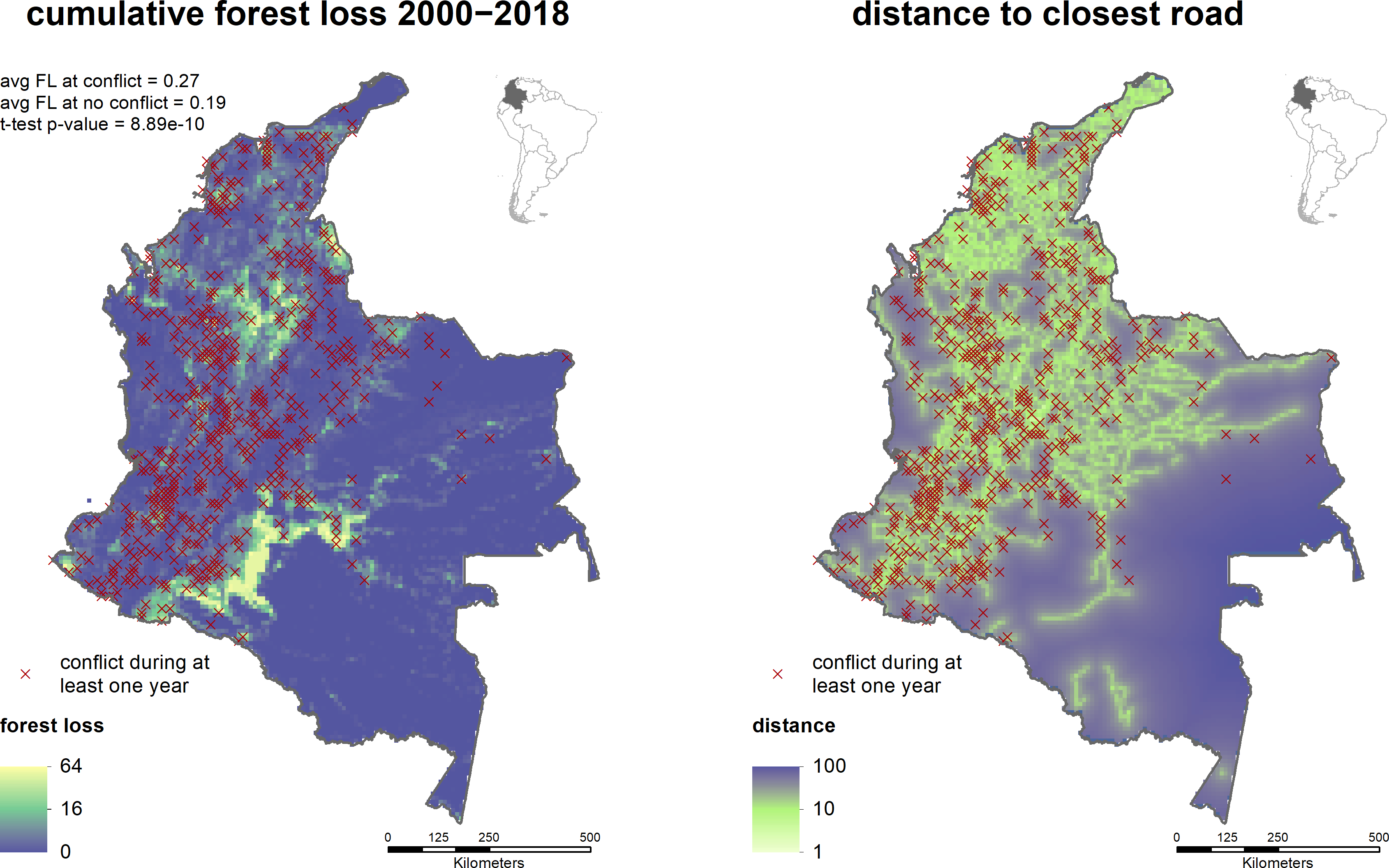
Figure 1: Temporally aggregated summary of the dataset described in Section 1.3. Conflicts are predictive of exceedances in forest loss (left), but this dependence is partly induced by a common dependence on accessibility, which we measure by the mean distance to a road (right). Failing to account for this variable and other confounders biases our estimate of the causal influence of conflict on forest loss.

A summary of the dataset can be seen in Figure 1. Visually, there is a strong positive dependence between the occurrence of a conflict and the loss of forest canopy. This observation is supported by simple summary statistics: the average forest loss across measurements classified as conflict events significantly exceeds that from non-conflict events by almost 50% (Figure 1, left), conforming previous findings [e.g., Landholm et al., 2019]. When seeking a causal explanation for the observed data, however, we regard such an analysis as flawed in two ways. First, both conflicts and forest loss predominantly occur in areas with high accessibility (Figure 1, right), indicating that the potential causal effect of $X$ on $Y$ is confounded by $W$. In fact, we expect the existence of several other confounders (e.g., population density, market infrastructure, etc.), many of which may be unobserved. Failing to account for confounding variables leads to biased estimates of the causal effect. Second, strong spatial dependencies in $X$ and $Y$ reduce the effective sample size, and a standard t-test thus exaggerates the significance of the observed difference in sample averages. To test hypotheses about $X$ and $Y$, we need statistical tests which are adapted to the spatio-temporal nature of data.

1.4 Contributions and structure of the paper

Apart from the case study, this paper contains three main theoretical contributions: the definition of a causal model for spatio-temporal data, a method for estimating causal effects (both Section 2), and a hypothesis test for the overall existence of such effects (Section 3). Section 4 applies our methodology to the above example. All data used for our analysis are publicly available. A description of how it can be obtained, along with an implementation of our method and reproducing scripts for all our figures and results, can be found at github.com/runesen/spatio_temporal_causality. All proofs are contained in Appendix H.

2 Quantifying causal effects for spatio-temporal data

A spatio-temporal dataset may be viewed as a single realization of a spatio-temporal stochastic process, observed at discrete points in space-time. In this section, we provide a formal framework to quantify causal relations among the components of a multivariate spatio-temporal process, and show how to estimate causal effects from observational data.

2.1 Causal models for spatio-temporal processes

Throughout this section, let $(\Omega,\mathcal{A},P)$ be some background probability space. A $p$-dimensional spatio-temporal process $\mathbf{Z}$ is a random variable taking values in the sample space $\mathcal{Z}_{p}$ of all $(\mathcal{B}(\mathbb{R}^{2}\times\mathbb{N}),\mathcal{B}(\mathbb{R}^{p}))$-measurable functions, where $\mathcal{B}(\cdot)$ denotes the Borel $\sigma$-algebra. We equip $\mathcal{Z}_{p}$ with the $\sigma$-algebra $\mathcal{F}_{p}$, defined as the smallest $\sigma$-algebra such that for all $B\in\mathcal{B}(\mathbb{R}^{p})$, the mapping $\mathcal{Z}_{p}\ni z\mapsto\int_{B}z(x)dx$ is $(\mathcal{F}_{p},\mathcal{B}(\mathbb{R}))$-measurable. The induced probability measure $\mathbb{P}$ on the measurable space $(\mathcal{Z}_{p},\mathcal{F}_{p})$, for every $F\in\mathcal{F}_{p}$ defined by $\mathbb{P}(F):=P(\mathbf{Z}^{-1}(F))$, is said to be the distribution of $\mathbf{Z}$. Throughout this paper, we use the notation $Z_{s}^{t}$ to denote the random vector obtained from marginalizing $\mathbf{Z}$ at location $s$ and time point $t$. We use $\mathbf{Z}_{s}$ for the time series $(Z_{s}^{t})_{t\in\mathbb{N}}$, $\mathbf{Z}^{t}$ for the spatial process $(Z_{s}^{t})_{s\in\mathbb{R}^{2}}$, and $\mathbf{Z}^{(S)}$ for the spatio-temporal process corresponding to the coordinates in $S\subseteq\{1,\dots,p\}$. We call a spatio-temporal process weakly stationary if the marginal distribution of $Z_{s}^{t}$ is the same for all $(s,t)\in\mathbb{R}^{2}\times\mathbb{N}$, and time-invariant if $\mathbb{P}(\mathbf{Z}^{1}=\mathbf{Z}^{2}=\cdots)=1$.

Multivariate spatio-temporal processes are used for the joint modeling of different phenomena, each of which corresponds to a coordinate process. Let us consider a decomposition of these coordinate processes into disjoint ‘bundles’. We are interested in specifying causal relations among these bundles while leaving the causal structure among variables within each bundle unspecified. Similarly to a graphical model [Lauritzen, 1996], our approach relies on a factorization of the joint distribution of $\mathbf{Z}$ into a number of components, each of which models the conditional distribution for one bundle given several others. This approach induces a graphical relation among the different bundles. We will equip these relations with a causal interpretation by additionally specifying the distribution of $\mathbf{Z}$ under certain interventions on the data generating process.

Definition 1 (Causal graphical models for spatio-temporal processes).

A causal graphical model for a $p$-dimensional spatio-temporal process $\mathbf{Z}$ is a triplet $(\mathcal{S},\mathcal{G},\mathcal{P})$ consisting of

• a family $\mathcal{S}=(S_{j})_{j=1}^{k}$ of non-empty, disjoint sets $S_{1},\dots,S_{k}\subseteq\{1,\dots,p\}$ with $\bigcup_{j=1}^{k}S_{j}=\{1,\dots,p\}$,

• a directed acyclic graph $\mathcal{G}$ with vertices $S_{1},\dots,S_{k}$, and

• a family $\mathcal{P}=(\mathcal{P}^{j})_{j=1}^{k}$ of collections $\mathcal{P}^{j}=\{\mathbb{P}^{j}_{z}\}_{z\in\mathcal{Z}_{\lvert\emph{PA}_{j}\rvert}}$ of distributions on $(\mathcal{Z}_{\lvert S_{j}\rvert},\mathcal{F}_{\lvert S_{j}\rvert})$, where for every $j$, $\emph{PA}_{j}:=\bigcup_{i:S_{i}\rightarrow S_{j}\in\mathcal{G}}S_{i}$. Whenever $\emph{PA}_{j}=\emptyset$, $\mathcal{P}^{j}$ consists only of a single distribution which we denote by $\mathbb{P}^{j}$.

Since $\mathcal{G}$ is acyclic, we can without loss of generality assume that $S_{1},\dots,S_{k}$ are indexed such that $S_{i}\not\to S_{j}$ in $\mathcal{G}$ whenever $i>j$. The above components induce a unique joint distribution $\mathbb{P}$ over $\mathbf{Z}$. For every $F=\bigtimes_{j=1}^{k}F_{j}$, it is defined by

$$\mathbb{P}(F)=\int_{F_{1}}\cdots\int_{F_{k}}\mathbb{P}_{z^{(\emph{PA}_{k})}}^{k}(dz^{(S_{k})})\cdots\mathbb{P}^{1}(dz^{(S_{1})}).$$ (1)

We call $\mathbb{P}$ the observational distribution. For each $j\in\{1,\dots,k\}$, the conditional distribution of $\mathbf{Z}^{(S_{j})}$ given $\mathbf{Z}^{(\emph{PA}_{j})}$ as induced by $\mathbb{P}$ equals $\mathcal{P}^{j}$. We define an intervention on $\mathbf{Z}^{(S_{j})}$ as replacing $\mathcal{P}^{j}$ by another model $\tilde{\mathcal{P}}^{j}$. This operation results in a new graphical model $(\mathcal{S},\mathcal{G},\tilde{\mathcal{P}})$ for $\mathbf{Z}$ which induces, via (1), a new distribution $\tilde{\mathbb{P}}$, the interventional distribution.

Assume that we perform an intervention on $\mathbf{Z}^{(S_{i})}$. By definition, the resulting interventional distribution differs from the observational distribution only in the way in which $\mathbf{Z}^{(S_{i})}$ depends on $\mathbf{Z}^{(\text{PA}_{i})}$, while all other conditional distributions $\mathbf{Z}^{(S_{j})}\,|\,\mathbf{Z}^{(\text{PA}_{j})}$, $j\not=i$, remain the same. This property is analogous to the modularity property of structural causal models [Haavelmo, 1944, Pearl, 2009, Peters et al., 2017] and justifies a causal interpretation of the conditionals in $\mathcal{P}$. We refer to the graph $\mathcal{G}$ as the causal structure of $\mathbf{Z}$, and sometimes write $\mathbf{Z}=[\mathbf{Z}^{(S_{k})}\,|\,\mathbf{Z}^{(\text{PA}_{k})}]\cdots[\mathbf{Z}^{(S_{1})}]$ to emphasize this structure.

2.2 Latent spatial confounder model

Motivated by the example introduced in Section 1.3, we are particularly interested in scenarios where a target variable $Y$ is causally influenced by a vector of covariates $X$, and where $(X,Y)$ are additionally affected by some latent variables $H$. In general, inferring causal effects under arbitrary influences of latent confounders is impossible, and we therefore need to impose additional restrictions on the variables in $H$. We here make the fundamental assumption that they do not vary across time (alternatively, one can assume that the hidden variables are invariant over space, see Appendix B.3).

Definition 2 (Latent spatial confounder model).

Consider a spatio-temporal process $(\mathbf{X},\mathbf{Y},\mathbf{H})=(X_{s}^{t},Y_{s}^{t},H_{s}^{t})_{(s,t)\in\mathbb{R}^{2}\times\mathbb{N}}$ over a real-valued response $Y$, a vector of covariates $X\in\mathbb{R}^{d}$ and a vector of latent variables $H\in\mathbb{R}^{\ell}$. We call a causal graphical model over $(\mathbf{X},\mathbf{Y},\mathbf{H})$ with causal structure $[\mathbf{Y}\,|\,\mathbf{X},\mathbf{H}][\mathbf{X}\,|\,\mathbf{H}][\mathbf{H}]$ a latent spatial confounder model (LSCM) if both of the following conditions hold true for the observational distribution.

• The latent process $\mathbf{H}$ is weakly stationary and time-invariant.

• There exists a measurable function $f:\mathbb{R}^{d+\ell+1}\to\mathbb{R}$ and an i.i.d. sequence $\boldsymbol{\varepsilon}^{1},\boldsymbol{\varepsilon}^{2},\dots$ of weakly-stationary spatial error processes, independent of $(\mathbf{X},\mathbf{H})$, such that

  $$Y_{s}^{t}=f(X_{s}^{t},H_{s}^{t},\varepsilon_{s}^{t})\qquad\text{ for all }(s,t)\in\mathbb{R}^{2}\times\mathbb{N}.$$ (2)

  We require that for all $x\in\mathbb{R}^{d}$, $f(x,H_{0}^{1},\varepsilon_{0}^{1})$ has finite expectation.

Throughout this section, we assume that $(\mathbf{X},\mathbf{Y},\mathbf{H})$ come from an LSCM. The above definition says that for every $s,t$, $Y_{s}^{t}$ depends on $(\mathbf{X},\mathbf{H})$ only via $(X_{s}^{t},H_{s}^{t})$, and that this dependence remains the same for all points in space-time. Together with the weak stationarity of $\mathbf{H}$ and $\boldsymbol{\varepsilon}$, this assumption ensures that the average causal effect of $X_{s}^{t}$ on $Y_{s}^{t}$ (which we introduce below) remains the same for all $s,t$. Our model class imposes no restrictions on the marginal distribution of $\mathbf{X}$. The spatial dependence structure of the error process $\boldsymbol{\varepsilon}$ must have the same marginal distributions everywhere, but is otherwise unspecified (in particular, $\boldsymbol{\varepsilon}$ is not required to be stationary). The temporal independence assumption on $\boldsymbol{\varepsilon}$ is necessary for our construction of resampling tests, see Section 3. We now formally define our inferential target.

Definition 3 (Average causal effect).

The average causal effect of $\mathbf{X}$ on $\mathbf{Y}$ is defined as the function $f_{\emph{AVE}(X\to Y)}:\mathbb{R}^{d}\to\mathbb{R}$, for every $x\in\mathbb{R}^{d}$ given by

$$f_{\emph{AVE}(X\to Y)}(x):=\mathbb{E}[f(x,H^{1}_{0},\varepsilon_{0}^{1})].$$ (3)

Here, the causal effect is an average effect in that it takes the expectation over both the noise variable (as opposed to making counterfactual statements [Rubin, 1974]) and the hidden variables. Alternatively, one may define the inferential target in terms of the single realization of $\mathbf{H}$ which manifested itself in the data, see Appendix C. The following proposition justifies $f_{\text{AVE}(X\to Y)}$ as a quantification of the causal influence of $\mathbf{X}$ on $\mathbf{Y}$.

Proposition 4 (Causal interpretation).

Let $(s,t)\in\mathbb{R}^{2}\times\mathbb{N}$ and $x\in\mathbb{R}^{d}$ be fixed, and consider any intervention on $\mathbf{X}$ such that $X_{s}^{t}=x$ holds almost surely in the induced interventional distribution $\mathbb{P}_{x}$. We then have that $\mathbb{E}_{\mathbb{P}_{x}}[Y_{s}^{t}]=f_{\emph{AVE}(X\to Y)}(x).$ That is, $f_{\emph{AVE}(X\to Y)}(x)$ is the expected value of $Y_{s}^{t}$ under any intervention that enforces $X_{s}^{t}=x$.

In many applications, we do not have explicit knowledge of, or data from, the interventional distributions $\mathbb{P}_{x}$. If we have access to the causal graph, however, we can sometimes compute intervention effects from the observational distribution. In the i.i.d. setting, depending on which variables are observed, this can be done by covariate adjustment or G-computation [Pearl, 2009, Rubin, 1974, Shpitser et al., 2010], for example. The following proposition shows a similar result in the case of an LSCM. It follows directly from Fubini’s theorem.

for all $s$, produce estimate $\hat{f}^{m}_{Y|X}(\mathbf{X}^{m}_{s},\mathbf{Y}^{m}_{s})(\cdot)$

Figure 2: Conceptual idea for estimating the average causal effect (green line) defined in (3). In both the left and right panel, we do not display time and space. The middle figure shows the data at different locations, i.e., every small plot corresponds to a single time series. The dashed curve illustrates the latent spatial confounder $H_{s}^{t}$ (for visual purposes, we here consider one-dim. space). Due to $H_{s}^{t}$, regressing $Y_{s}^{t}$ on $X_{s}^{t}$ (red line in left plot) leads to a biased estimator. Our estimator (blue line in right plot) removes this bias. The procedure is shown in the middle figure: for all $s$, we observe several instances $(X_{s}^{t},Y_{s}^{t})$, $t=1,\dots,m$, with the same conditionals $Y_{s}^{t}\,|\,(X_{s}^{t},H^{t}_{s})$ and the same (unobserved) value of $H_{s}^{t}$. For each realization $h_{s}$ of $H^{1}_{s}$, we can thus estimate the regression $f_{Y|(X,H)}(\cdot,h_{s})$ only using the data $(\mathbf{X}_{s}^{m},\mathbf{Y}_{s}^{m})$ (blue lines in middle figure). A final estimate of the average causal effect (blue line in right plot) is obtained by approximating the expectation in (5) by a sample average over all spatial locations, see Section 2.3.

Proposition 5 (Covariate adjustment).

Let $f_{Y|(X,H)}$ denote the regression function $(x,h)\mapsto\mathbb{E}[Y_{s}^{t}\,|\,X_{s}^{t}=x,H_{s}^{t}=h]$ (by definition of an LSCM, this function is the same for all $s,t$). For all $x\in\mathbb{R}^{d}$, it holds that

$$f_{\emph{\text{AVE}}(X\to Y)}(x)=\mathbb{E}[f_{Y|(X,H)}(x,H_{0}^{1})].$$ (4)

Proposition 5 shows that $f_{\text{AVE}(X\to Y)}$ is identified from the full observational distribution over $(\mathbf{X},\mathbf{Y},\mathbf{H})$ (given that the LSCM structure is known). Since $\mathbf{H}$ is unobserved, the main challenge is to estimate (4) merely based on data from $(\mathbf{X},\mathbf{Y})$, see Section 2.3. (We discuss in Appendix B.1 how to furthermore include observable time-varying covariates.)

2.3 Estimation of the average causal effect

2.3.1 Definition and consistency

In practice, we only observe the process $(\mathbf{X},\mathbf{Y})$ at a finite number of points in space and time. We assume that at every temporal instance, we observe the process at the same spatial locations $s_{1},\dots,s_{n}\in\mathbb{R}^{2}$ (these locations need not lie on a regular grid). To simplify notation, we furthermore assume that the observed time points are $t=1,2,\ldots,m$, i.e., we have access to a dataset $(\mathbf{X}_{n}^{m},\mathbf{Y}_{n}^{m})=(X_{s}^{t},Y_{s}^{t})_{(s,t)\in\{s_{1},\dots,s_{n}\}\times\{1,\dots,m\}}$. The proposed method is based on the following key idea: for every $s\in\{s_{1},\dots,s_{n}\}$, we observe several time instances $(X_{s}^{t},Y_{s}^{t})$, $t\in\{1,\dots,m\}$, all with the same conditionals $Y_{s}^{t}\,|\,(X_{s}^{t},H^{t}_{s})$. Since $\mathbf{H}$ is time-invariant, we can, for every $s$, estimate $f_{Y|(X,H)}(\cdot,h_{s})$ for the (unobserved) realization $h_{s}$ of $H^{1}_{s}$ using the data $(X_{s}^{t},Y_{s}^{t})$, $t\in\{1,\dots,m\}$. The expectation in (4) is then approximated by averaging estimates obtained from different spatial locations. This idea is visualized in Figure 2. More formally, our method requires as input a model class for the regressions $f_{Y|(X,H)}(\cdot,h)$, $h\in\mathbb{R}^{\ell}$, alongside with a suitable estimator $\hat{f}_{Y|X}=(\hat{f}^{m}_{Y|X})_{m\in\mathbb{N}}$, and returns

$$\hat{f}^{nm}_{\text{AVE}(X\rightarrow Y)}(\mathbf{X}_{n}^{m},\mathbf{Y}_{n}^{m})(x):=\frac{1}{n}\sum_{i=1}^{n}\hat{f}^{m}_{Y|X}(\mathbf{X}^{m}_{s_{i}},\mathbf{Y}^{m}_{s_{i}})(x),$$ (5)

an estimator of the average causal effect (3) within the given model class. In Section 3, we furthermore provide a statistical test for the overall existence of a causal effect. Our approach may be seen as summarizing the output of a spatially varying regression model [e.g., Gelfand et al., 2003] that is allowed to change arbitrarily from one location to the other (within the model class dictated by $\hat{f}_{Y|X}$). By permitting such flexibility, our method does not rely on observing data from a continuous or spatially connected domain, and accommodates complex influences of the latent variables. An implementation can be found in our code package, see Section 1.4.

To prove consistency of our estimator, we let the number of observable points in space-time increase. Let therefore $(s_{n})_{n\in\mathbb{N}}\subseteq\mathbb{R}^{2}$ be a sequence of spatial coordinates, and consider the array of data $(\mathbf{X}_{n}^{m},\mathbf{Y}_{n}^{m})_{n,m\geq 1}$, where for every $n,m\in\mathbb{N}$, $(\mathbf{X}_{n}^{m},\mathbf{Y}_{n}^{m})=(X_{s}^{t},Y_{s}^{t})_{(s,t)\in\{s_{1},\dots,s_{n}\}\times\{1,\dots,m\}}$. We want to prove that the corresponding sequence of estimators (5) consistently estimates (3). To obtain such a result, we need two central assumptions.

Assumption A1 (LLN for the latent process).

For all measurable functions $\varphi:\mathbb{R}^{\ell}\to\mathbb{R}$ with $\mathbb{E}[\lvert\varphi(H_{0}^{1})\rvert]<\infty$ it holds that $\tfrac{1}{n}\sum_{i=1}^{n}\varphi(H^{1}_{s_{i}})\to\mathbb{E}[\varphi(H_{0}^{1})]$ in probability as $n\to\infty$.

Assumption A1 ensures that, for an increasing number of spatial locations at which data are observed, the spatial average in (5) approximates the expectation in (3). The assumption is satisfied, for example, for a stationary Gaussian process $\mathbf{H}^{1}$ that is sampled regularly across an increasing spatial domain, see Proposition 10 in Appendix D. As the number of observed time points tends to infinity, we furthermore require the estimators $\hat{f}^{m}_{Y|X}$ to converge to the integrand in (3), at least in some area $\mathcal{X}\subseteq\mathbb{R}^{d}$.

Assumption A2 (Consistent estimators of the conditional expectations).

There exists $\mathcal{X}\subseteq\mathbb{R}^{d}$ such that for all $x\in\mathcal{X}$ and $s\in\mathbb{R}^{2}$, it holds that $\hat{f}^{m}_{Y|X}(\mathbf{X}_{s}^{m},\mathbf{Y}_{s}^{m})(x)-f_{Y|(X,H)}(x,H_{s}^{1})\to 0$, in probability as $m\to\infty$.

A slightly stronger, but maybe more intuitive formulation is to require the above consistency to hold conditionally on $\mathbf{H}$, i.e., assuming that for all $x\in\mathcal{X}$, $s\in\mathbb{R}^{2}$ and almost all $\mathbf{h}$, $\hat{f}^{m}_{Y|X}(\mathbf{X}_{s}^{m},\mathbf{Y}_{s}^{m})(x)\to f_{Y|(X,H)}(x,h_{s}^{1})$ as $m\to\infty$, in probability under $\mathbb{P}(\cdot\,|\,\mathbf{H}=\mathbf{h})$. It follows from the dominated convergence theorem that this assumption implies Assumption A2. Under Assumptions A1 and A2, we obtain the following consistency result.

Theorem 6 (Consistent estimator of the average causal effect).

Let $(\mathbf{X},\mathbf{Y},\mathbf{H})$ come from an LSCM as defined in Definition 2. Let $(s_{n})_{n\in\mathbb{N}}$ be a sequence of spatial coordinates such that the marginalized process $(H^{1}_{s_{n}})_{n\in\mathbb{N}}$ satisfies Assumption A1, and assume that for all $x\in\mathcal{X}$, $\mathbb{E}[\lvert f_{Y|(X,H)}(x,H_{0}^{1})\rvert]<\infty$. Let furthermore $\hat{f}_{Y|X}=(\hat{f}^{m}_{Y|X})_{m\in\mathbb{N}}$ be an estimator satisfying Assumption A2. We then have the following consistency result. For all $x\in\mathcal{X}$, $\delta>0$ and $\alpha>0$, there exists $N\in\mathbb{N}$ such that for all $n\geq N$ we can find $M_{n}\in\mathbb{N}$ such that for all $m\geq M_{n}$ we have that

$$\mathbb{P}\left(\left|\hat{f}^{nm}_{\emph{AVE}(X\rightarrow Y)}(\mathbf{X}_{n}^{m},\mathbf{Y}_{n}^{m})(x)-f_{\emph{AVE}(X\rightarrow Y)}(x)\right|>\delta\right)\leq\alpha.$$ (6)

Apart from the LSCM structure, the above result does not rely on any particular distributional properties of the data. Assumptions A1 and A2 do not impose strong restrictions on the data generating process and hold true for several model classes, including linear and nonlinear models. In Appendix D, we provide sufficient conditions under which these assumptions are true.

2.3.2 An example LSCM

To illustrate the consistency result in Theorem 6, we now consider a simple example with one covariate ($d=1$) and two hidden variables ($\ell=2$).

Example 7 (Latent Gaussian process and a linear average causal effect).

Let $\boldsymbol{\zeta},\boldsymbol{\psi},\boldsymbol{\xi}^{t},\boldsymbol{\varepsilon}^{t}$, $t\in\mathbb{N}$, be independent versions of a univariate stationary spatial Gaussian process with mean $0$ and covariance function $u\mapsto e^{-\tfrac{1}{2}\lVert u\rVert_{2}}$. For notational simplicity, let $\bar{\mathbf{H}}$ and $\tilde{\mathbf{H}}$ denote the respective first and second coordinate process of $\mathbf{H}$. We define a marginal distribution over $\mathbf{H}$ and conditional distributions $\mathbf{X}\,|\,\mathbf{H}$ and $\mathbf{Y}\,|\,(\mathbf{X},\mathbf{H})$ by specifying that for all $(s,t)\in\mathbb{R}^{2}\times\mathbb{N}$,

$$H_{s}^{t} =(\bar{H}_{s}^{t},\tilde{H}_{s}^{t})=(\zeta_{s},1+\tfrac{1}{2}\zeta_{s}+\tfrac{\sqrt{3}}{2}\psi_{s}),$$

$$X_{s}^{t} =\exp(-\lVert s\rVert_{2}^{2}/1000)+(0.2+0.1\cdot\sin(2\pi t/100))\cdot\bar{H}_{s}^{t}\cdot\tilde{H}_{s}^{t}+0.5\cdot\xi_{s}^{t},$$

$$Y_{s}^{t} =(1.5+\bar{H}_{s}^{t}\cdot\tilde{H}_{s}^{t})\cdot X_{s}^{t}+(\bar{H}_{s}^{t})^{2}+\lvert\tilde{H}_{s}^{t}\rvert\cdot\varepsilon_{s}^{t}.$$

Interventions on $\mathbf{X}$, $\mathbf{Y}$ or $\mathbf{H}$ are defined as in Definition 1. In this LSCM, the average causal effect $f_{\emph{AVE}(X\to Y)}$ is the linear function $x\mapsto\beta_{0}+\beta_{1}x$, with $\beta_{0}:=\mathbb{E}[(\bar{H}_{0}^{1})^{2}]=1$ and $\beta_{1}:=1.5+\mathbb{E}[\bar{H}_{0}^{1}\cdot\tilde{H}_{0}^{1}]=2$. We define a spatial sampling scheme $(s_{i})_{i\in\mathbb{N}}$ for every $j\in\mathbb{N}$ and $k\in\{1,\dots,25\}$ by $s_{25\cdot(j-1)+k}=(j,k)$. Given a sample $(\mathbf{X}_{n}^{m},\mathbf{Y}_{n}^{m})=(X_{s}^{t},Y_{s}^{t})_{(s,t)\in\{s_{1},\dots,s_{n}\}\times\{1,\dots,m\}}$ from $(\mathbf{X},\mathbf{Y})$, we construct an estimator of $f_{\emph{AVE}(X\to Y)}$ by

$$\hat{f}_{\emph{AVE}(X\to Y)}^{nm}(\mathbf{X}_{n}^{m},\mathbf{Y}_{n}^{m})(x)=\frac{1}{n}\sum_{i=1}^{n}(1\ x)\,\hat{\beta}_{\emph{OLS}}^{m}(\mathbf{X}_{s_{i}}^{m},\mathbf{Y}_{s_{i}}^{m}),$$ (7)

where $\hat{\beta}_{\emph{OLS}}^{m}(\mathbf{X}_{s_{i}}^{m},\mathbf{Y}_{s_{i}}^{m})\in\mathbb{R}^{2}$ is the OLS estimator for the linear regression at spatial location $s_{i}$, that is of $\mathbf{Y}_{s_{i}}^{m}=(Y_{s_{i}}^{1},\ldots,Y_{s_{i}}^{m})$ on $\mathbf{X}_{s_{i}}^{m}=(X_{s_{i}}^{1},\ldots,X_{s_{i}}^{m})$ (we assume that the regression includes an intercept term). It follows by Propositions 10 and 11 (see in particular Example 13 and Remark 15 in Appendix E) that Assumptions A1 and A2 are satisfied. Hence, (7) is a consistent estimator of $f_{\emph{AVE}(X\to Y)}$.

Figure 3 illustrates our procedure using a numerical experiment based on Example 7. The example shows that we can estimate causal effects even under complex influences of the latent process $\mathbf{H}$. To construct the estimator $\hat{f}_{\text{AVE}(X\to Y)}^{nm}$, we have used that the influence of $(\mathbf{X},\mathbf{H})$ on $\mathbf{Y}$ is linear in $\mathbf{X}$. However, we do not assume knowledge of the particular functional dependence of $\mathbf{Y}$ on $\mathbf{H}$; we obtain consistency under any influence of the form $Y_{s}^{t}=f_{1}(H_{s}^{t})\cdot X_{s}^{t}+f_{2}(H_{s}^{t},\varepsilon_{s}^{t})$, see Proposition 11.

$\bar{\mathbf{H}}$     $\tilde{\mathbf{H}}$     $\mathbf{X}$     $\mathbf{Y}$

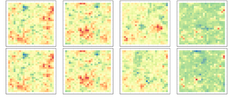
$\vdots$       $\vdots$       $\vdots$       $\vdots$

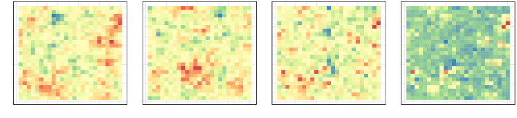
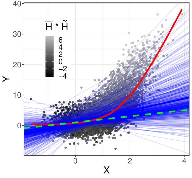
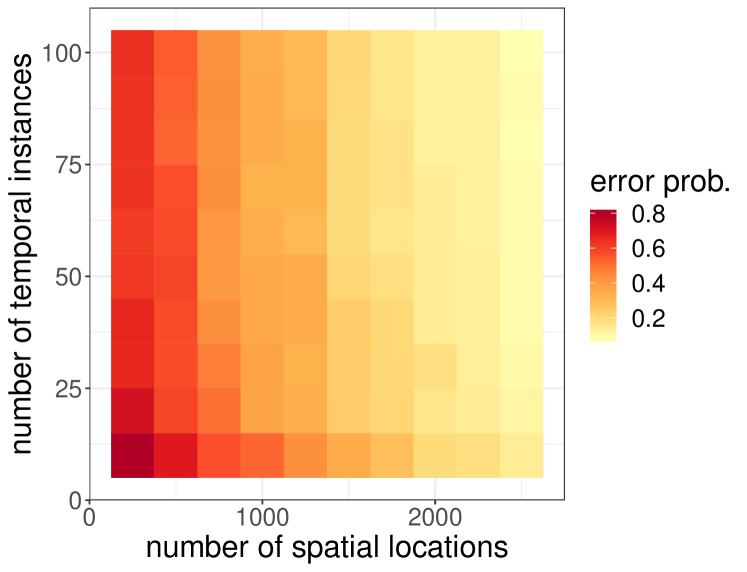
Figure 3: Results for applying our methodology to Example 7. The left panel shows a sample dataset of $(\mathbf{X},\mathbf{Y},\mathbf{H})$ observed at the spatial grid $\{1,\dots,25\}^{2}$ and at several time instances. The middle panel illustrates our method applied to the same dataset. The average causal effect, our inferential target, is indicated by a green line. Due to confounding by $H_{s}^{t}$, a standard nonlinear regression (red curve) severely overestimates the causal influence of $X_{s}^{t}$ on $Y_{s}^{t}$. By regressing $Y_{s}^{t}$ on $X_{s}^{t}$ in each location separately (thin blue lines), and aggregating the results into a final estimate (thick blue line), all spatial confounding is removed. In the right panel, we investigate the consistency result from Theorem 6 empirically. For increasing $n$ and $m$, we generate several datasets $(\mathbf{X}_{n,i}^{m},\mathbf{Y}_{n,i}^{m})$, $i=1,\dots,100$, compute estimates $\hat{\beta}^{nm}_{i}$ of the causal coefficients $\beta$, and use these to compute empirical error probabilities $\hat{\mathbb{P}}(\lVert\hat{\beta}^{nm}-\beta\rVert_{2}>\delta)$. In the above plot, we have chosen $\delta=0.2$. As $n$ and $m$ increase, the error probability tends towards zero.

2.3.3 Extensions

Our methodology can be extended in several directions. In Appendix B, we provide details on how to model the influence of observed (time- and space-varying) confounders and temporally lagged causal effects of $\mathbf{X}$ on $\mathbf{Y}$. We furthermore argue that our method also applies in situations where the roles of time and space are interchanged, i.e., when the hidden confounders are time-varying, but remain static across space. The extension which includes observed confounders is furthermore explored empirically in Appendix F.1.

3 Testing for the existence of causal effects

The previous section has been concerned with the quantification and estimation of the causal effect of $X$ on $Y$. In this section, we introduce hypothesis tests for this effect being zero. We consider the null hypothesis

$$H_{0}:(\mathbf{X},\mathbf{Y})\text{ come from an LSCM with a function }f\text{ that is constant w.r.t.\ }X_{s}^{t},$$

which formalizes the assumption of “no causal effect of $X$ on $Y$” within the LSCM framework. We construct a hypothesis test for $H_{0}$ using data resampling. Our approach acknowledges the existence of spatial dependence in the data without modeling it explicitly. It thus does not rely on distributional assumptions apart from the LSCM structure.

For the construction of a resampling test, we closely follow the setup presented in Pfister et al. [2018]. We require a data permutation scheme which, under the null hypothesis, leaves the distribution of the data unaffected. In particular, it must preserve the dependence between $\mathbf{X}$ and $\mathbf{Y}$ that is induced by $\mathbf{H}$. The idea is to permute observations of $\mathbf{Y}$ corresponding to the same (unobserved) values of $\mathbf{H}$. Since $\mathbf{H}$ is assumed to be constant within every spatial location, this is achieved by permuting $\mathbf{Y}$ along the time axis. Let $(\mathbf{X}_{n}^{m},\mathbf{Y}_{n}^{m})$ be the observed data. For every $(\mathbf{x},\mathbf{y})\in\mathbb{R}^{(d+1)\times n\times m}$ and every permutation $\sigma$ of the elements in $\{1,\dots,m\}$, let $\sigma(\mathbf{x},\mathbf{y})\in\mathbb{R}^{(d+1)\times n\times m}$ denote the permuted array with entries $(\sigma(x,y))^{t}_{s}=(x_{s}^{t},y_{s}^{\sigma(t)})$. We then have the following exchangeability property.

Proposition 8 (Exchangeability).

For any permutation $\sigma$ of the elements in $\{1,\dots,m\}$, we have that, under $H_{0}$, $\sigma(\mathbf{X}_{n}^{m},\mathbf{Y}_{n}^{m})$ is equal in distribution to $(\mathbf{X}_{n}^{m},\mathbf{Y}_{n}^{m})$.

Proposition 8 is the cornerstone for the construction of a valid resampling test. Under the null hypothesis, we can compute pseudo-replications of the observed sample $(\mathbf{X}_{n}^{m},\mathbf{Y}_{n}^{m})$ using the permutation scheme described above. Given any test statistic $\hat{T}:\mathbb{R}^{(d+1)\times n\times m}\to\mathbb{R}$, we obtain a $p$-value for $H_{0}$ by comparing the value of $\hat{T}$ calculated on the original dataset with the empirical null distribution of $\hat{T}$ obtained from the resampled datasets. The choice of $\hat{T}$ determines the power of the test. More formally, let $M:=m!$ and let $\sigma_{1},\dots,\sigma_{M}$ be all permutations of the elements in $\{1,\dots,m\}$. By Proposition 8, each $\sigma_{i}$ yields a new dataset with the same distribution as $(\mathbf{X}_{n}^{m},\mathbf{Y}_{n}^{m})$. Let $B\in\mathbb{N}$ and let $k_{1},\dots,k_{B}$ be independent, uniform draws from $\{1,\dots,M\}$. For every $(\mathbf{x},\mathbf{y})$, we define

$$p_{\hat{T}}(\mathbf{x},\mathbf{y}):=\frac{1+\lvert\{b\in\{1,\dots,B\}:\hat{T}(\sigma_{k_{b}}(\mathbf{x},\mathbf{y}))\geq\hat{T}(\mathbf{x},\mathbf{y})\}\rvert}{1+B},$$

and construct for every $\alpha\in(0,1)$ a test $\varphi_{\hat{T}}^{\alpha}:\mathbb{R}^{(d+1)\times n\times m}\to\{0,1\}$ of $H_{0}$ defined by $\varphi^{\alpha}_{\hat{T}}=1:\Leftrightarrow p_{\hat{T}}\leq\alpha$. The following level guarantee for $\varphi_{\hat{T}}^{\alpha}$ follows directly from [Pfister et al., 2018, Proposition B.4].

Corollary 9 (Level guarantee of resampling test).

Assume that for all $k,\ell\in\{1,\dots,B\}$, $k\not=\ell$, it holds that, under $H_{0}$, $\mathbb{P}(\hat{T}(\sigma_{k}(\mathbf{X}_{n}^{m},\mathbf{Y}_{n}^{m}))=\hat{T}(\sigma_{\ell}(\mathbf{X}_{n}^{m},\mathbf{Y}_{n}^{m})))=0$. Then, for every $\alpha\in(0,1)$, the test $\varphi_{\hat{T}}^{\alpha}$ has correct level $\alpha$.

Corollary 9 ensures valid test level for a large class of test statistics. The particular choice of test statistic should depend on the alternative hypothesis that we seek to have power against. Within the LSCM model class, it makes sense to quantify deviations from the null hypothesis using functionals of the average causal effect, i.e., $T=\psi(f_{\text{AVE}(X\to Y)})$ for some suitable function $\psi$. As a test statistic, we then use the plug-in estimator $\hat{T}(\mathbf{X}_{n}^{m},\mathbf{Y}_{n}^{m})=\psi(\hat{f}^{nm}_{\text{AVE}(X\to Y)}(\mathbf{X}_{n}^{m},\mathbf{Y}_{n}^{m})).$ An implementation of the above testing procedure is contained in our code package, see Section 1.4. A power-analysis can be found in Appendix F.3.

4 Conflict and forest loss in Colombia

We return to the problem of conflict ($\mathbf{X}$) and forest loss ($\mathbf{Y}$). As discussed in Section 1.3, there may exist several confounders of the (potential) causal effect of $\mathbf{X}$ on $\mathbf{Y}$. We believe that many of these vary at a relatively low temporal frequency (e.g., population density, market infrastructure), justifying the application of the methods developed above.

4.1 Data description and preprocessing

Our analysis is based on two main datasets: (1) a remote sensing-based forest loss dataset for the period 2000–2018, which identifies annual forest loss at a spatial resolution of $30$\mathrm{m}$\times 30$\mathrm{m}$$ using Landsat satellites [Hansen et al., 2013]. Here, forest loss is defined as complete canopy removal. (2) Spatially explicit information on conflict events from 2000 to 2018, based on the Georeferenced Event Dataset (GED) from the Uppsala Conflict Data Program (UCDP) [Croicu and Sundberg, 2015]. In this dataset, a conflict event is defined as “an incident where armed force was used by an organized actor against another organized actor, or against civilians, resulting in at least one direct death at a specic location and a specifc date”. Such events were identified through global newswire reporting, global monitoring of local news, and other secondary sources such as reports by non-governmental organizations (for information on the data collection as well as control for quality and consistency of the data, please refer to Croicu and Sundberg [2015]). We homogenized these datasets through aggregation to a spatial resolution of $10$\mathrm{km}$\times 10$\mathrm{km}$$ by averaging the annual forest loss within each grid, and by counting all conflict events occurring in the same year and within the same grid. As a proxy for accessibility, we additionally calculated, for each spatial grid, the average Euclidean distance to the closest road segment, using spatial data from https://diva-gis.org containing all primary and secondary roads in Colombia. We regard this variable as relatively constant throughout the considered time-span.

4.2 Quantifying the causal influence of conflict on forest loss

We assume that $(\mathbf{X},\mathbf{Y})$ come from an LSCM as defined in Defintion 2. Since $X_{s}^{t}$ is binary, we can characterize the causal influence of $\mathbf{X}$ on $\mathbf{Y}$ by $T:=f_{\text{AVE}(X\to Y)}(1)-f_{\text{AVE}(X\to Y)}(0)$, i.e., the difference in expected forest loss $\mathbb{E}[Y_{s}^{t}]$ under the respective interventions enforcing conflict ($X_{s}^{t}:=1$) and peace ($X_{s}^{t}:=0$). Positive values of $T$ correspond to an augmenting effect of conflict on forest loss and negative values correspond to a reducing effect. Our goal is to estimate $T$, and to test the hypothesis $H_{0}:T=0$ (no causal effect of $\mathbf{X}$ on $\mathbf{Y}$). To construct an estimator of the average causal effect of the form (5), we require estimators of the conditional expectations $x\mapsto f_{Y|(X,H)}(x,h)$. Since $X_{s}^{t}$ is binary, we use simple sample averages of the response variable. To make the resulting estimator of $f_{\text{AVE}(X\to Y)}$ well-defined, we omit all locations which do not contain at least one observation from each of the regimes $X_{s}^{t}=0$ and $X_{s}^{t}=1$. More precisely, let $(\mathbf{X}_{n}^{m},\mathbf{Y}_{n}^{m})$ be the observed dataset. We then use the estimator

$$\hat{f}^{nm}_{\text{AVE}(X\to Y)}(\mathbf{X}_{n}^{m},\mathbf{Y}_{n}^{m})(x)=\frac{1}{\lvert\mathcal{I}_{n}^{m}\rvert}\sum_{i\in\mathcal{I}_{n}^{m}}\frac{1}{\lvert\{t:X_{s_{i}}^{t}=x\}\rvert}\sum_{t:X_{s_{i}}^{t}=x}Y_{s_{i}}^{t},\qquad x\in\{0,1\},$$ (8)

where $\mathcal{I}_{n}^{m}:=\{i\in\{1,\dots,n\}\,:\,\exists\ t_{0},t_{1}\in\{1,\dots,m\}\text{ such that }X_{s_{i}}^{t_{0}}=0\text{ and }X_{s_{i}}^{t_{1}}=1\}$. To test $H_{0}$, we use the resampling test from Section 3 with $\hat{T}=\hat{f}^{nm}_{\text{AVE}(X\to Y)}(1)-\hat{f}^{nm}_{\text{AVE}(X\to Y)}(0)$. In Appendix F.4, we argue that, under additional assumptions on the underlying LSCM, the above estimator is approximately unbiased. Note, however, that even if the above estimator is biased, this does not affect the level guarantee of our testing procedure—we obtain a valid test level for any test statistic $\hat{T}$ satisfying the assumptions of Corollary 9.

4.3 Alternative assumptions on the causal structure

To emphasize the relevance of the assumed causal structure, we compare our method with two alternative approaches based on different assumptions about the ground truth: Model 1 assumes no confounders of $(\mathbf{X},\mathbf{Y})$ and Model 2 assumes that the only confounder is the observed process $\mathbf{W}$ (mean distance to a road). In reality, we expect the existence of several confounders in addition to $\mathbf{W}$, e.g., population density or market infrastructure. Even though none of the models may be a precise description of the data generating mechanism, we therefore regard both Models 1 and 2 as less realistic than the LSCM. In both models we can, similarly to Definition 3, define the average causal effect of $\mathbf{X}$ on $\mathbf{Y}$. Under Model 1, $f_{\text{AVE}(X\to Y)}$ coincides with the conditional expectation of $Y_{s}^{t}$ given $X_{s}^{t}$, which can be estimated simply using sample averages (as is done in Figure 1 left). Under Model 2, $f_{\text{AVE}(X\to Y)}$ can, analogously to Proposition 5, be computed by adjusting for the confounder $\mathbf{W}$. For each $x\in\{0,1\}$, we obtain an estimate $\hat{f}^{nm}_{\text{AVE}(X\to Y)}(x)$ by calculating sample averages of $\mathbf{Y}$ across different subsets $\{(s,t)\in\mathbb{R}^{2}\times\mathbb{N}\,:\,X_{s}^{t}=x,\,W_{s}^{t}\in\mathcal{W}_{j}\},j\in\mathcal{J}$ (we here construct these by considering 100 equidistant quantiles of $\mathbf{W}$), and subsequently averaging over the resulting values. In both models, we furthermore test the hypothesis of no causal effect of $\mathbf{X}$ on $\mathbf{Y}$ using approaches similar to the ones presented in Section 3. Under the LSCM assumption, we have constructed a permutation scheme that permutes the values of $\mathbf{Y}$ along the time axis, to preserve the dependence between $\mathbf{Y}$ and $\mathbf{H}$, see Proposition 8. Similarly, we construct a permutation scheme for Model 2 by permuting observations of $\mathbf{Y}$ corresponding to similar values of the confounder $\mathbf{W}$ (i.e., values within the same quantile range). Under the null hypothesis corresponding to Model 1, $\mathbf{X}$ and $\mathbf{Y}$ are (unconditionally) independent, and we therefore permute the values of $\mathbf{Y}$ completely at random. Strictly speaking, the permutation schemes for Models 1 and 2 require additional exchangeability assumptions on $\mathbf{Y}$ in order to yield valid tests. In Appendix G, we repeat the analysis for Model 1 using a spatial block-permutation to account for the spatial dependence in $\mathbf{Y}$, and obtain similar results.

4.4 Results

The results of applying our method and the two alternative approaches to the entire study region are depicted in Figure 4. Under Model 1, there is an enhancing, highly significant causal effect of conflict on forest loss ($\hat{T}=0.073$, $P=0.002$). When adjusting for accessibility (quantified by $\mathbf{W}$, Model 2), the size of the estimated causal effect shrinks, and becomes insignificant ($\hat{T}=0.049$, $P=0.168$). (Note that we have considered other confounders, too, yet obtained similar results. For example, when adjusting for population density, which we consider as moderately temporally varying, we obtain $\hat{T}=0.038$ and $P=0.214$.) When applying the methodology proposed in this paper, that is, adjusting for all time-invariant confounders, the estimated effect swaps sign ($\hat{T}=-0.018$, $P=0.578$), but is insignificant. We also tested for spatial spill-over effects by modeling causal effects that are spatially lagged by up to one or two pixels, respectively. In both cases, the effect was negative and insignificant (results not shown here). One reason for the above non-finding could be the time delay between the proposed cause (conflict) and effect (forest loss). To account for this potential issue, we also test for a causal effect of $\mathbf{X}$ on $\mathbf{Y}$ that is temporally lagged by one year, i.e., we use an estimator similar to (8), where we compare the average forest loss succeeding conflict events with the average forest loss succeeding non-conflict events. Again, the estimated influence of $\mathbf{X}$ on $\mathbf{Y}$ is negative and insignificant ($\hat{T}=-0.0293$, $P=0.354$). Additionally, we perform alternative versions of the last two tests to account for potential autocorrelation in the response variable, by adopting a temporal block-permutation scheme. In both cases, the test is insignificant, see Appendix G.

$H_{0}:$

Model 1

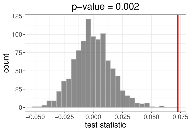
Model 2

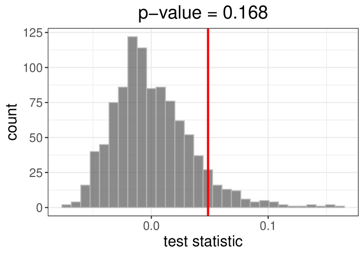
LSCM

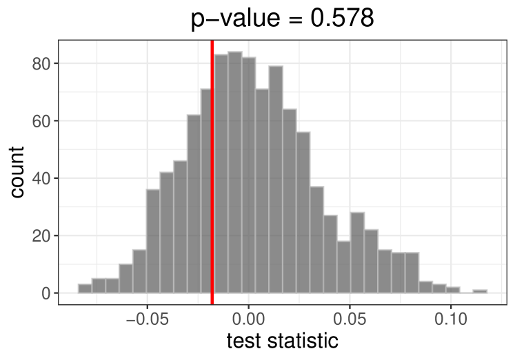
Figure 4: Testing for a causal influence of conflict ($\mathbf{X}$) on forest loss ($\mathbf{Y}$) using our method (right) and two alternative approaches (left and middle) which are based on different and arguably less realistic assumptions on the causal structure. The process $\mathbf{W}$ corresponds to the mean distance to a road, and $\mathbf{H}$ represents unobserved time-invariant confounders. Each of the above models gives rise to a different expression for the test statistic $\hat{T}=\hat{f}^{nm}_{\text{AVE}(X\to Y)}(1)-\hat{f}^{nm}_{\text{AVE}(X\to Y)}(0)$ (indicated by red vertical bars), see Sections 4.2 and 4.3. The gray histograms illustrate the empirical null distributions of $\hat{T}$ under the respective null hypotheses obtained from 999 resampled datasets. The results show that our conclusions about the causal influence of conflict on forest loss strongly depend on the assumed causal structure: under Model 1, there is a positive, highly significant effect ($\hat{T}=0.073$). When adjusting for the confounder $\mathbf{W}$, the effect size decreases and becomes insignificant ($\hat{T}=0.049$). When applying our proposed methodology, the estimated effect is negative ($\hat{T}=-0.018$).

The above analysis provides an estimate for the average causal effect, see Equation (3), which, in particular, averages over space. Given that Colombia is a country with high ambiental and socio-economic heterogeneity, we furthermore conduct an analysis at the department level (see Figure 5). In fact, there is considerable spatial variation in the estimated causal effects, with significant positive as well as negative effects (Figure 5 middle). This variation may be seen as evidence for an interaction effect between conflict and the assumed hidden confounders. In most departments, the estimated causal effect is negative (although mostly insignificant), meaning that conflict tends to decrease forest loss. The strongest positive and significant causal influence is identified in the La Guajira department ($\hat{T}=0.398$, $P=0.047$). Although this region is commonly associated with semi-arid to very dry conditions, most conflicts occured in the South-Western areas, at the beginning of Caribbean tropical forests (see Figure 1). In fact, these zones have also been also identified by Negret et al. [2019] as having been strongly affected by deforestation pressure in the wake of conflict. Interestingly, the neighboring Magdalena department shows the opposite effect ($\hat{T}=-0.218$, $P=0.004$). The positive effect in the department of Huila ($\hat{T}=0.095$, $P=0.023$) is again in line with the findings by Negret et al. [2019] (based on a visual inspection of their attribution maps). Out of the 8 departments that are mostly controlled by FARC (Figure 5 right), 6 have a negative test statistic, meaning that conflict reduces forest loss. This can be explained in part by the internal governance of this group, where forest cover was a strategic advantage for both their own protection as well as for cocaine production. Overall, of course, the peace-induced acceleration of forest loss has to be discussed with caution, and should not be interpreted reversely as if conflict per se is a measure of environmental protection Clerici et al. [2020].

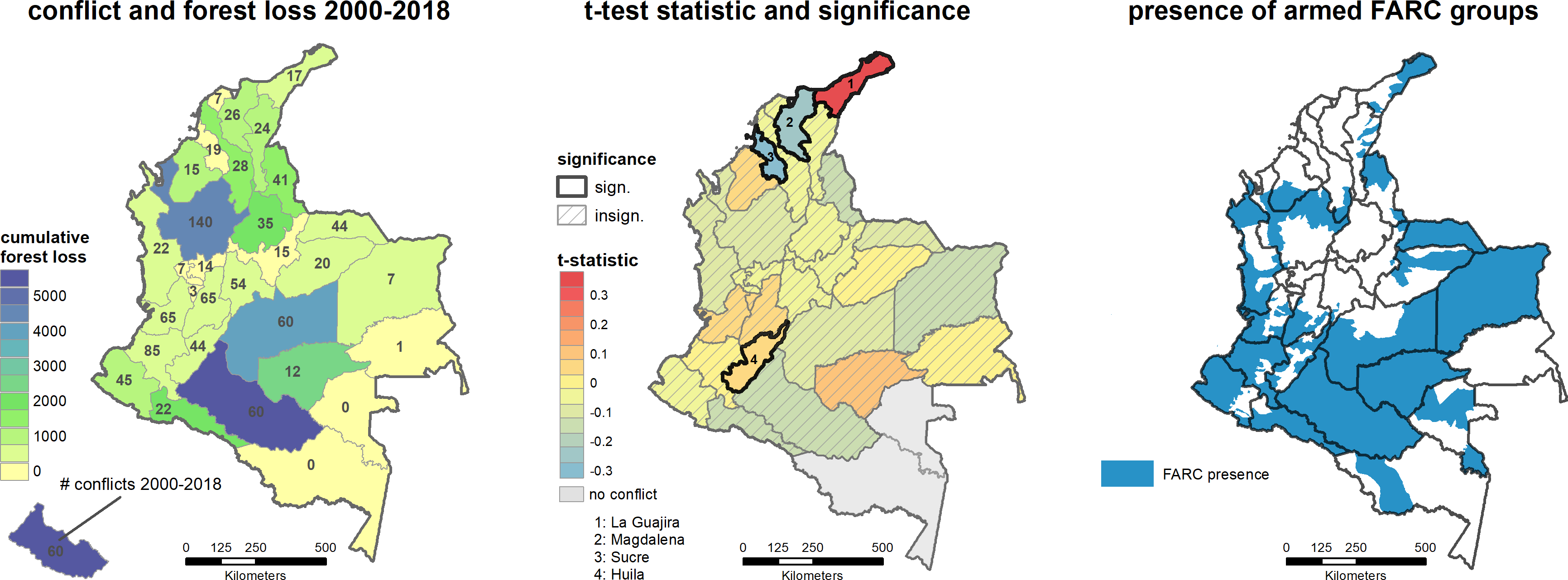
Figure 5: Regional analysis of conflict and forest loss in Colombia. The left panel shows the total forest loss and the total number of conflict events 2000–2018 at department level. The most severe incidences of forest loss occur in the northern Andean forests and on the northern borders of the Amazon region. In the middle panel, we report for each department estimates $\hat{T}$ and test results for $H_{0}:T=0$, using the methodology described in Sections 2 and 3. We used a test level of $\alpha=0.05$, and report significances without multiple-testing adjustment. In most departments, the estimated causal effect is negative (blue, conflict reduces forest loss), although mainly insignificant. We identify four departments with statistically significant results, hereof two with a positive causal effect (La Guarija and Huila) and two with a negative causal effect (Magdalena and Sucre). In total, there are 8 departments that are mostly controlled by FARC (above 75% FARC presence, right panel). Out of these, 6 departments have a negative test statistic (conflict reduces forest loss).

4.5 Interpretation in light of the Colombian peace process

In late 2012, negotiations that later would be known as the ‘Colombian peace process’ started between the then president of Colombia and the strongest group of rebels, the FARC, lasting until 2016. Peace was declared by both parties upon a revised agreement in October 2016, and became effective in 2017. The negotiations marked a steadily decreasing number of conflicts (Figure 6, left). Since this decrease is the result of governmental intervention, rather than a natural resolution of local tensions, the peace process provides an opportunity to verify the intervention effects estimated in Section 4.4. As can be seen in Figure 6 (right), Colombia experienced a steep increase in the total forest loss in the final phase of the peace negotiations. Although there may be several other factors which have contributed to this development, we observe that these results align with our previous finding of an overall negative causal effect of conflict on forest loss ($\hat{T}<0$).

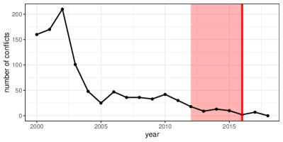
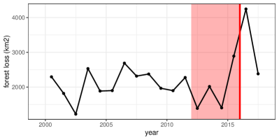
Figure 6: Number of conflicts (left) and forest loss (right) in the years 2000–2018 in Colombia. In the right panel, the height of the curve at $x+0.5$ indicates the forest loss between years $x$ and $x+1$. Shaded areas mark the Colombian peace process (2012–2016).

5 Conclusions and future work

5.1 Methodology

This paper introduces ways to discuss causal inference for spatio-temporal data. From a methodological perspective, it contains three main contributions: the definition of a class of causal models for multivariate spatio-temporal stochastic processes, a procedure for estimating causal effects within this model class, and a non-parametric hypothesis test for the overall existence of such effects. Our method allows for the influence of arbitrarily many latent confounders, as long as these confounders do not vary across time (or space). We prove asymptotic consistency of our estimator, and verify this finding empirically using simulated data. Our results hold under weak assumptions on the data generating process, and do not rely on any particular distributional properties of the data. We prove sufficient conditions under which these rather general assumptions hold true. The proposed testing procedure is based on data resampling and provably obtains valid level in finite samples.

Our work can be extended into several directions. We proved that Assumption A1 holds for regularly sampled stationary Gaussian processes. Such settings allow for the application of well-known theorems about stationary and ergodic sequences. We hypothesize that the assumption also holds in the more general case, where the marginalized process does not resemble a (collection of) stationary sequence(s), as long certain mixing conditions are satisfied. For example, we believe that if the original spatial process $\mathbf{H}^{1}$ is weakly stationary and mixing, Assumption A1 holds under any spatial sampling scheme $(s_{n})_{n\in\mathbb{N}}$ with $\lVert s_{n}\rVert_{2}\to\infty$ as $n\to\infty$.

Our method assumes that all latent confounders are time-invariant. It would be interesting to see whether the error of our estimation procedure can be bounded when, violating the assumptions, there are unobserved, time-varying confounders, but such confounders vary only slowly over time. Likewise, it would be worthwile exploring how smoothness assumptions on the spatial variation of the hidden variables can be incorporated in the modeling process to gain statistical efficiency of our estimator. Such smoothness assumptions would also allow for alternative permutation schemes (data can be permuted spatially wherever $\mathbf{H}$ is assumed to be constant) which could lead to increased power of our hypothesis tests.

5.2 Case study

We have applied our methodology to the problem of conflict and forest loss in Colombia. Conflicts are predictive of exceedances in forest loss, but we find no evidence of a causal relation when analyzing this problem on country level: once all (time-invariant) confounders are adjusted for, there is a negative but insignificant correlation between conflict and forest loss. Our analysis on department level suggests that this non-finding could be due to locally varying effects of opposite directionality, which would approximately cancel out in our final estimate. In most departments, we find negative (mostly insignificant) effects, although we also identify a few departments where conflict seems to increase forest loss. It would be interesting to further explore these differences in causal dependence, e.g., by adjusting for socio-political factors. The overall negative influence of conflict on forest loss estimated by our method is in line with the observation that during the final phase of the peace process, which stopped many of the existing conflicts, the total forest loss in Colombia has increased. However, these results should be interpreted with caution. Overall, we find that, once all time-invariant confounders are adjusted for, conflicts have only weak explanatory power for predicting forest loss, and the potential causal effect is therefore likely to be small, compared to other drivers of forest loss. Further, our results rely on the assumption that all latent confounders are time-invariant, which, in practice, can only be expected to hold approximately. In Appendix F.1, we explore how our estimator is affected by temporal variation in the latent confounders.

Appendix A Existing causal methodology

For independent and identically distributed (i.i.d.) and time series data, that is, for data, for which the spatial information can be neglected, causal models have been well-studied. Among the most widely used approaches are structural causal models, causal graphical models, and the framework of potential outcomes [see, e.g., Bollen, 2014, Pearl, 2009, Peters et al., 2017, Rubin, 1974]. Knowledge of the causal structure of a system does not only provide us with cause-effect relationships; sometimes, it also allows us to quantify causal relations by estimating intervention effects from observational data. If, for example, we know that $W$ is causing $X$ and $Y$, and that $X$ is causing $Y$, procedures such as variable adjustment can be used to estimate the causal influence of $X$ on $Y$ from i.i.d. replications [Pearl, 2009, Rubin, 1974]. While using a slightly different language, the same underlying causal deliberations are the basis of many works in econometrics, e.g., work related to generalized methods of moments and identifiability of parameters [e.g., Hansen, 1982, Newey and McFadden, 1994]. In this field, data are often assumed to have a time series structure [e.g., Hall, 2005].

For spatio-temporal data, several methods have been proposed [e.g., Lozano et al., 2009, Luo et al., 2013]. These are mostly algorithmical approaches that extend the concept of Granger causality [Granger, 1980, Wiener, 1956] to spatio-temporal data. They reduce the question of causality to predictability and a positive time lag. In particular, these methods assume that there are no relevant unobserved variables (‘confounders’) and they do not resolve the question of time-instantaneous causality between different points in space. More classical approaches for causal inference [e.g., Peirce, 1883, Rosenbaum and Rubin, 1983, Kelejian et al., 2004, Delgado and Florax, 2015] require either a controlled study design, data from all confounding variables, a valid instrument, or a naturally occurring experiment, respectively, and are therefore not applicable to the case study considered in this paper. Furthermore, to the best of our knowledge, existing work does not provide a formal model for causality for spatio-temporal data. As a consequence, the precise definition of the target of inference, the causal effect, remains vague.

Appendix B Extensions of our methodology

B.1 Observed time-varying confounders

For simplicity, we have until now assumed that the only confounders of $(X,Y)$ are the variables in $H$. Our method naturally extends to settings with observed (time- and space-varying) confounders. Let $W\in\mathbb{R}^{p}$ be some observed covariates, and consider a causal graphical model over $(\mathbf{X},\mathbf{W},\mathbf{Y},\mathbf{H})$ with causal structure $[\mathbf{Y}\,|\,\mathbf{X},\mathbf{W},\mathbf{H}][\mathbf{X}\,|\,\mathbf{W},\mathbf{H}][\mathbf{W},\mathbf{H}]$. Similarly to Definition 2, assume that $\mathbf{W}$ and $\mathbf{H}$ are weakly stationary, $\mathbf{H}$ is time-invariant, and there exists a function $f:\mathbb{R}^{d+p+\ell+1}\to\mathbb{R}$ and an i.i.d. sequence $\boldsymbol{\varepsilon}^{1},\boldsymbol{\varepsilon}^{2},\dots$ of weakly stationary error processes, independent of $(\mathbf{X},\mathbf{W},\mathbf{H})$, such that

$$Y_{s}^{t}=f(X_{s}^{t},W_{s}^{t},H_{s}^{t},\varepsilon_{s}^{t})\quad\text{ for all }(s,t)\in\mathbb{R}^{2}\times\mathbb{N}.$$ (9)

We define the average causal effect of $\mathbf{X}$ on $\mathbf{Y}$, for every $x\in\mathbb{R}^{d}$, by

$$f_{\text{AVE}(X\to Y)}(x)=\mathbb{E}[f(x,W_{0}^{1},H_{0}^{1},\varepsilon_{0}^{1})].$$

It is straight-forward to show that this function enjoys the same causal interpretation as given in Proposition 4. Similarly to Proposition 5, $f_{\text{AVE}(X\to Y)}$ can be recovered from the full observational distribution over $(X_{0}^{1},W_{0}^{1},Y_{0}^{1},H_{0}^{1})$ by conditioning on $(X_{0}^{1},W_{0}^{1},H_{0}^{1})$, followed by taking the expectation w.r.t. $(W_{0}^{1},H_{0}^{1})$. More precisely, we have

$$f_{\text{AVE}(X\to Y)}(x) =\int_{\mathbb{R}^{p+\ell}}f_{Y|(X,W,H)}(x,w,h)\mathbb{P}_{(W,H)}(d(w,h))$$

$$=\int_{\mathbb{R}^{\ell}}\int_{\mathbb{R}^{p}}f_{Y|(X,W,H)}(x,w,h)\mathbb{P}_{W|(H=h)}(dw)\mathbb{P}_{H}(dh),$$

where $f_{Y|(X,W,H)}$ is the regression function of $Y_{s}^{t}$ onto $(X_{s}^{t},W_{s}^{t},H^{t}_{s})$. Motivated by the above equation, we estimate $f_{\text{AVE}(X\to Y)}$ by first estimating the regression function $f_{Y|(X,W,H)}$, and then approximating the two integrals. Since $\mathbf{H}$ is time-invariant, we can, similarly to (5), use the estimator

$$\hat{f}^{nm}_{\text{AVE}(X\rightarrow Y)}(\mathbf{X}_{n}^{m},\mathbf{Y}_{n}^{m},\mathbf{W}_{n}^{m})(x):=\frac{1}{n}\sum_{i=1}^{n}\hat{\mathbb{E}}_{s_{i}}[\hat{f}^{m}_{Y|(X,W)}(\mathbf{X}^{m}_{s_{i}},\mathbf{Y}^{m}_{s_{i}},\mathbf{W}_{s_{i}}^{m})(x,W_{0}^{1})],$$ (10)

where $\hat{f}^{m}_{Y|(X,W)}(\mathbf{X}^{m}_{s_{i}},\mathbf{Y}^{m}_{s_{i}},\mathbf{W}_{s_{i}}^{m})$ is an estimate of $(x,w)\mapsto f_{Y|(X,W,H)}(x,w,h_{s_{i}})$ computed from the observed data at location $s_{i}$, and $\hat{\mathbb{E}}_{s_{i}}$ is the expectation w.r.t. the empirical distribution of $\mathbf{W}_{s_{i}}^{m}$ (which serves as an approximation of the inner integral).

B.2 Temporally lagged causal effects

We can incorporate temporally lagged causal effects by allowing the function $f$ in (2) to depend on past values of the predictors. That is, we model a joint causal influence of the past $k\geq 1$ temporal instances of the predictors by assuming the existence of a function $f:\mathbb{R}^{d\cdot k+\ell+1}\to\mathbb{R}$ and an i.i.d. sequence $\boldsymbol{\varepsilon}^{1},\boldsymbol{\varepsilon}^{2},\dots$ such that

$$Y_{s}^{t}=f(X_{s}^{t-k+1},\dots,X_{s}^{t},H_{s}^{t},\varepsilon_{s}^{t})\quad\text{ for all }s\in\mathbb{R}^{2}\text{ and }t\geq k.$$

In this case, the average causal effect (3) is a function $\mathbb{R}^{d\cdot k}\to\mathbb{R}$ which can be estimated, similarly to (5), using a regression estimator $\hat{f}^{m}_{Y|X}$ of $Y_{s}^{t}$ onto $(X_{s}^{t-k+1},\dots,X_{s}^{t})$.

B.3 Exchanging the role of space and time

We have assumed that the hidden confounders do not vary across time. This assumption allowed us to estimate the regression $x\mapsto\mathbb{E}[Y_{s}^{t}\,|\,X_{s}^{t}=x,H_{s}^{t}=h]$ at all unobserved values $h$. In fact, our method can be formulated in more general terms. If $(\mathbf{X},\mathbf{Y},\mathbf{H})$ is a multivariate process defined on some general, possibly random, index set $\mathcal{I}=I_{1}\times\cdots\times I_{p}$ (see the definition of a data cube [Mahecha et al., 2020]), it is enough to require $\mathbf{H}$ to be invariant across one (or several) of the dimensions in $\mathcal{I}$. Similarly to (5), the idea is then to estimate the dependence of $\mathbf{Y}$ on $(\mathbf{X},\mathbf{H})$ along these invariant dimensions, followed by an aggregation across the remaining dimensions. In case of a spatio-temporal process, for example, our method also applies if the hidden variables are constant across space, rather than time.

Appendix C Alternative definition of the average causal effect

In our definition of the average causal effect (3), we take the expectation with respect to the hidden variables $H$. By the assumption of time-invariance, however, there is only a single replication of the spatial process $\mathbf{H}^{1}$. One may argue that it is more relevant to define the inferential target in terms of that one realization, rather than in terms of a distribution over possible alternative outcomes which will never manifest themselves. This leads to the alternative definition of the average causal effect

$$x\mapsto\lim_{S\to\infty}\frac{1}{(2S)^{2}}\int_{[-S,S]^{2}}\mathbb{E}[f(x,h^{1}_{s},\varepsilon_{0}^{1})]\,ds=\lim_{S\to\infty}\frac{1}{(2S)^{2}}\int_{[-S,S]^{2}}f_{Y|(X,H)}(x,h^{1}_{s})\,ds,$$

assuming that the above limits exist. Under the assumption of ergodicity of $\mathbf{H}^{1}$, the above expression coincides with Definition 3, but it is learnable from data, via the estimator introduced in Section 2.3, even if this is not the case. Here, we choose the formulation in Definition 3 because we found that it results in a more comprehensible theory.

Appendix D Sufficient conditions for Assumptions A1 and A2

For Assumption A1, we consider a stationary Gaussian setup. By considering a regular spatial sampling scheme, we can make use of standard ergodic theorems for stationary and ergodic time series.

Proposition 10 (Sufficient conditions for Assumption A1).

Assume that $\mathbf{H}^{1}$ is a stationary multivariate Gaussian process with covariance function $C:\mathbb{R}^{2}\to\mathbb{R}^{\ell\times\ell}$, i.e., $C(h)=\emph{Cov}(H^{1}_{s},H^{1}_{s+h})$ for all $s,h\in\mathbb{R}^{2}$. Assume that $C(h)\to 0$ entrywise as $\lVert h\rVert_{2}\to\infty$. Consider a regular grid $\{s^{1}_{1},s^{1}_{2},\dots\}\times\{s^{2}_{1},s^{2}_{2},\dots,s^{2}_{m}\}\subseteq\mathbb{R}^{2}$, where $s^{1}_{1}<s^{1}_{2}<\cdots$ are equally spaced, and let $(s_{n})_{n\in\mathbb{N}}$ be the spatial sampling scheme for every $i\in\mathbb{N}$ and $j\in\{1,\dots,m\}$ given as $s_{(i-1)m+j}=(s^{1}_{i},s^{2}_{j})$. Then, the process $(H^{1}_{s_{n}})_{n\in\mathbb{N}}$ satisfies Assumption A1.

The proof of the above proposition uses mixing conditions on the sequence $(H^{1}_{s_{n}})_{n\in\mathbb{N}}$, which rely on the fact that $\lVert s_{n}\rVert_{2}\to\infty$. In spatial statistics, these types of asymptotic regimes are known as ‘increasing domain asymptotics’. To ensure Assumption A1 in a setting where $(s_{n})_{n\in\mathbb{N}}$ corresponds to an increasingly fine sampling of some bounded domain (‘in-fill asymptotics’), we believe that a different set of assumptions on the process $\mathbf{H}^{1}$ would be necessary.

For Assumption A2, we consider the slightly stronger version formulated conditionally on $\mathbf{H}$. We let $\mathcal{H}\subseteq\mathcal{Z}_{\ell}$ denote the set of all functions $\mathbf{h}:\mathbb{R}^{2}\times\mathbb{N}\to\mathbb{R}^{\ell}$ that are constant in the time-argument. Since $\mathbf{H}$ is time-invariant, we have that $\mathbb{P}(\mathbf{H}\in\mathcal{H})=1$, and it therefore suffices to prove the statement for all $\mathbf{h}\in\mathcal{H}$. Below, we use, for every $\mathbf{h}\in\mathcal{H}$, $\mathbb{P}_{\mathbf{h}}$ to denote the conditional distribution $\mathbb{P}(\cdot\,|\,\mathbf{H}=\mathbf{h})$ and $\mathbb{E}_{\mathbf{h}}$ for the expectation with respect to $\mathbb{P}_{\mathbf{h}}$.

We now make some structural assumptions on the function $f$ in (2), which allow us to parametrically estimate the regressions $x\mapsto f_{Y|(X,H)}(x,h)$. Let $\{\varphi_{1},\dots,\varphi_{p}\}$ be a known basis of continuous functions on $\mathbb{R}^{d}$, and with $\varphi_{1}\equiv 1$ an intercept term. With $\varphi:=(\varphi_{1},\dots,\varphi_{p})$, we make the following assumptions on the underlying LSCM.

• There exist functions $f_{1}:\mathbb{R}^{\ell}\to\mathbb{R}^{p}$ and $f_{2}:\mathbb{R}^{\ell+1}\to\mathbb{R}$ such that Equation (2) splits into

  $$Y_{s}^{t}=\varphi(X_{s}^{t})^{\top}f_{1}(H_{s}^{t})+f_{2}(H_{s}^{t},\varepsilon_{s}^{t})\qquad\text{ for all }(s,t)\in\mathbb{R}^{2}\times\mathbb{N},$$

  and such that for all $h\in\mathbb{R}^{\ell}$, $f_{2}(h,\varepsilon_{0}^{1})$ has finite second moment.

For every $s,t$, define $\xi_{s}^{t}=f_{2}(H_{s}^{t},\varepsilon_{s}^{t})$. We can w.l.o.g. assume that for all $s$, $t$ and $h$, $\mathbb{E}[\xi_{s}^{t}\,|\,H_{s}^{t}=h]=0$. (Since $\varphi_{1}\equiv 1$, this can always be accommodated by adding $h\mapsto\mathbb{E}[\xi_{s}^{t}\,|\,H_{s}^{t}=h]$ to the first coordinate of $f_{1}$.) For every fixed $\mathbf{h}\in\mathcal{H}$ and $s\in\mathbb{R}^{2}$, assumption (L1) says that, under $\mathbb{P}_{\mathbf{h}}$, $(\mathbf{X}_{s},\mathbf{Y}_{s})$ follows a simple regression model, where $\mathbb{E}[Y_{s}^{t}\,|\,X_{s}^{t}]$ depends linearly on $\varphi(X_{s}^{t})$. For arbitrary but fixed $h_{s}^{1}$, we can therefore estimate $x\mapsto\mathbb{E}[Y_{s}^{1}\,|\,X_{s}^{1}=x,H_{s}^{1}=h_{s}^{1}]$ using standard OLS estimation. For every $s\in\mathbb{R}^{2}$ and $m\in\mathbb{N}$, let $\mathbf{\Phi}_{s}^{m}\in\mathbb{R}^{m\times p}$ be the design matrix given by $(\mathbf{\Phi}_{s}^{m})_{ij}=\varphi_{j}(X_{s}^{i})$. We define an estimator $\hat{f}_{Y|X}=(\hat{f}^{m}_{Y|X})_{m\in\mathbb{N}}$, for every $x\in\mathbb{R}^{d}$ and $m\in\mathbb{N}$ by

$$\hat{f}^{m}_{Y|X}(\mathbf{X}_{s}^{m},\mathbf{Y}_{s}^{m})(x)=\varphi(x)^{\top}\hat{\gamma}_{s}^{m},$$ (11)

where $\hat{\gamma}_{s}^{m}:=((\mathbf{\Phi}_{s}^{m})^{\top}\mathbf{\Phi}_{s}^{m})^{-1}(\mathbf{\Phi}_{s}^{m})^{\top}\mathbf{Y}_{s}^{m}.$ To formally prove consistency of (11), we need some regularity conditions on the predictors $\mathbf{X}$.

• For all $\mathbf{h}\in\mathcal{H}$, $s\in\mathbb{R}^{2}$ and $\delta>0$, it holds that

  $$\lim_{m\to\infty}\mathbb{P}_{\mathbf{h}}(\lVert\tfrac{1}{m}(\mathbf{\Phi}_{s}^{m})^{\top}\boldsymbol{\xi}_{s}^{m}\rVert_{2}>\delta)=0.$$

• For all $\mathbf{h}\in\mathcal{H}$, $s\in\mathbb{R}^{2}$, there exists $c>0$ such that

  $$\lim_{m\to\infty}\mathbb{P}_{\mathbf{h}}(\lambda_{\text{min}}\left(\tfrac{1}{m}(\mathbf{\Phi}_{s}^{m})^{\top}\mathbf{\Phi}_{s}^{m}\right)\leq c)=0,$$

  where $\lambda_{\text{min}}$ denotes the minimal eigenvalue.

We first state the result and discuss assumptions (L2) and (L3) afterwards.

Proposition 11 (Sufficient conditions for Assumption A2).

Assume that $(\mathbf{X},\mathbf{Y},\mathbf{H})$ come from an LSCM satisfying (L1)–(L3). Then, Assumption A2 is satisfied with $\mathcal{X}=\mathbb{R}^{d}$ and with $\hat{f}^{m}_{Y|X}$ as defined in (11).

Since for every $(s,t)\in\mathbb{R}^{2}\times\mathbb{N}$ and $\mathbf{h}\in\mathcal{H}$, $X_{s}^{t}$ and $\xi_{s}^{t}$ are independent under $\mathbb{P}_{\mathbf{h}}$ with $\mathbb{E}_{\mathbf{h}}[\xi_{s}^{t}]=0$, (L2) states a natural LLN-type condition, which is satisfied under suitable constraints on the temporal dependence structure in $\mathbf{X}$, and on its variance. Assumption (L3) says that, with probability tending to one, the matrix $\tfrac{1}{m}(\mathbf{\Phi}_{s}^{m})^{\top}\mathbf{\Phi}_{s}^{m}$ is bounded away from singularity as $m\to\infty$. This is in particular satisfied if $\tfrac{1}{m}(\mathbf{\Phi}_{s}^{m})^{\top}\mathbf{\Phi}_{s}^{m}$ converges in probability entrywise to some matrix which is strictly positive definite. In Appendix E, we give two examples in which this is the case.

Appendix E Examples satisfying conditions L1 and L2

Let $(\mathbf{X},\mathbf{Y},\mathbf{H})$ come from an LSCM satisfying condition (L1) described in Appendix D. Below, we give two examples of distributions over $(\mathbf{X},\mathbf{H})$ for which also conditions (L2) and (L3) hold true. In both cases, $\tfrac{1}{m}(\mathbf{\Phi}_{s}^{m})^{\top}\mathbf{\Phi}_{s}^{m}$ converges in probability to some limit matrix of the form $\mathbb{E}_{\nu}[\varphi(X)\varphi(X)^{\top}]$ for some measure $\nu$ with full support on $\mathbb{R}^{d}$. To see that $\mathbb{E}_{\nu}[\varphi(X)\varphi(X)^{\top}]$ is strictly positive definite, let $v\in\mathbb{R}^{p}$ be such that $0=v^{\top}\mathbb{E}_{\nu}[\varphi(X)\varphi(X)^{\top}]v=\mathbb{E}_{\nu}[\lVert\varphi(X)^{\top}v\rVert_{2}^{2}]$. By continuity of $\varphi$, it follows that $\varphi^{\top}v\equiv 0$, and the linear independence of $\varphi_{1},\dots,\varphi_{p}$ implies that $v=0$.

Example 12 (Temporally ergodic $\mathbf{X}$).

Let $(\mathbf{X},\mathbf{Y},\mathbf{H})$ come from an LSCM satisfying Assumption (L1). Assume that for every $\mathbf{h}\in\mathcal{H}$ and $s\in\mathbb{R}^{2}$, it holds that under $\mathbb{P}_{\mathbf{h}}$, $\mathbf{X}_{s}$ is a stationary and mixing process with a marginal distribution that has full support on $\mathbb{R}^{d}$ (e.g., a vector autoregessive process with additive Gaussian noise). Assume furthermore that $\mathbb{E}_{\mathbf{h}}[\lvert\xi_{s}^{1}\rvert^{2}]<\infty$ and $\mathbb{E}_{\mathbf{h}}[\lvert\varphi_{i}(X_{s}^{1})\rvert^{2}<\infty]$ for all $i\in\{1,\dots,p\}$. Analogously to the proof of Proposition 10, we can then show that for each $i,j\in\{1,\dots,p\}$, the sequences $(\varphi_{i}(X_{s}^{t})\xi_{s}^{t})_{t\in\mathbb{N}}$ and $(\varphi_{i}(X_{s}^{t})\varphi_{j}(X_{s}^{t}))_{t\in\mathbb{N}}$ are ergodic under $\mathbb{P}_{\mathbf{h}}$, and it follows that

$$(\tfrac{1}{m}(\mathbf{\Phi}_{s}^{m})^{\top}\boldsymbol{\xi}_{s}^{m})_{i}=\frac{1}{m}\sum_{t=1}^{m}\varphi_{i}(X_{s}^{t})\xi_{s}^{t}\to\mathbb{E}_{\mathbf{h}}[\varphi_{i}(X_{s}^{1})\xi_{s}^{1}]$$

and

$$(\tfrac{1}{m}(\mathbf{\Phi}_{s}^{m})^{\top}\mathbf{\Phi}_{s}^{m})_{ij}=\frac{1}{m}\sum_{t=1}^{m}\varphi_{i}(X_{s}^{t})\varphi_{j}(X_{s}^{t})\to\mathbb{E}_{\mathbf{h}}[\varphi_{i}(X_{s}^{1})\varphi_{j}(X_{s}^{1})]$$

as $m\to\infty$ in probability under $\mathbb{P}_{\mathbf{h}}$. Since for all $s\in\mathbb{R}^{2}$, $\mathbb{E}_{\mathbf{h}}[\varphi(X_{s}^{1})\xi_{s}^{1}]=\mathbb{E}_{\mathbf{h}}[\varphi(X_{s}^{1})]\cdot\mathbb{E}_{\mathbf{h}}[\xi_{s}^{1}]=0$ and $\mathbb{E}_{\mathbf{h}}[\varphi(X_{s}^{1})\varphi(X_{s}^{1})^{\top}]\succ 0$, the above implies (L2) and (L3).

Example 13 (Temporally independent $\mathbf{X}$ with convergent mixture distributions).

Let $(\mathbf{X},\mathbf{Y},\mathbf{H})$ come from an LSCM satisfying Assumption (L1) for some bounded functions $\varphi_{1},\dots,\varphi_{p}$. Assume that for every $s\in\mathbb{R}^{2}$, the variables $X_{s}^{1},X_{s}^{2},\dots$ are conditionally independent given $\mathbf{H}$ (they are not required to be identically distributed), and that for every $\mathbf{h}\in\mathcal{H}$, the sequence of mixture distributions

$$\mathbb{P}_{s,\mathbf{h}}^{m}:=\frac{1}{m}\sum_{t=1}^{m}\mathbb{P}_{X_{s}^{t}|\mathbf{H}=\mathbf{h}},\quad m\in\mathbb{N},$$ (12)

converges, for $m\rightarrow\infty$, weakly towards some limit measure $\mathbb{P}_{s,\mathbf{h}}^{\infty}$ with full support on $\mathbb{R}^{d}$. Then, conditions (L1) and (L2) are satisfied. To see this, let $\mathbf{h}\in\mathcal{H}$ and $s\in\mathbb{R}^{2}$ be fixed for the rest of this example. Let $m\in\mathbb{N}$ and $\delta>0$. Since $\mathbb{E}_{\mathbf{h}}[(\mathbf{\Phi}_{s}^{m})^{\top}\boldsymbol{\xi}_{s}^{m}]=0$, it follows from Chebychev’s inequality that for all $i\in\{1,\dots,p\}$,

$$\mathbb{P}_{\mathbf{h}}(\lvert\tfrac{1}{m}((\mathbf{\Phi}_{s}^{m})^{\top}\boldsymbol{\xi}_{s}^{m})_{i}\rvert>\delta)\leq\frac{1}{\delta^{2}}\emph{Var}_{\mathbf{h}}(\frac{1}{m}((\mathbf{\Phi}_{s}^{m})^{\top}\boldsymbol{\xi}_{s}^{m})_{i})=\frac{\mathbb{E}_{\mathbf{h}}((\xi_{0}^{1})^{2})}{\delta^{2}m}\underbrace{\mathbb{E}_{s,\mathbf{h}}^{m}[\varphi_{i}(X)^{2}]}_{\emph{unif. bounded}}\to 0,$$

as $m\to\infty$, showing that (L2) is satisfied. To prove (L3), let $M^{m}:=\mathbb{E}_{s,\mathbf{h}}^{m}[\varphi(X)\varphi(X)^{\top}]$, $m\in\mathbb{N}$, and $M^{\infty}:=\mathbb{E}_{s,\mathbf{h}}^{\infty}[\varphi(X)\varphi(X)^{\top}]$ (to simplify notation, we here omit the implicit dependence on $\mathbf{h}$ and $s$). By assumption on $(\mathbb{P}_{s,\mathbf{h}}^{m})_{m\in\mathbb{N}}$, $M^{m}$ converges entrywise to $M^{\infty}$ as $m\to\infty$. Together with another application of Chebychev’s inequality, it follows that for all $i,j\in\{1,\dots,p\}$,

$$\mathbb{P}_{\mathbf{h}}(\lvert\tfrac{1}{m}((\mathbf{\Phi}_{s}^{m})^{\top}\mathbf{\Phi}_{s}^{m})_{ij}-M^{\infty}_{ij}\rvert>2\delta) \leq\mathbb{P}_{\mathbf{h}}(\lvert\tfrac{1}{m}((\mathbf{\Phi}_{s}^{m})^{\top}\mathbf{\Phi}_{s}^{m})_{ij}-M^{m}_{ij}\rvert>\delta)+\mathbb{P}_{\mathbf{h}}(\lvert M^{m}_{ij}-M^{\infty}_{ij}\rvert>\delta)$$

$$\leq\frac{1}{\delta^{2}m}\underbrace{\mathbb{E}_{s,\mathbf{h}}^{m}[\varphi_{i}(X)^{2}\varphi_{j}(X)^{2}]}_{\emph{unif. bounded}}+\underbrace{\mathbb{P}_{\mathbf{h}}(\lvert M^{m}_{ij}-M^{\infty}_{ij}\rvert>\delta)}_{=0\emph{ for }m\emph{ large}}$$

$$\to 0\quad\text{ as }m\to\infty,$$

showing that $\tfrac{1}{m}((\mathbf{\Phi}_{s}^{m})^{\top}\mathbf{\Phi}_{s}^{m})$ converges entrywise to $M^{\infty}\succ 0$ in probability under $\mathbb{P}_{\mathbf{h}}$, and (L3) follows.

Remark 14 (Necessity of the convergence of mixtures).

The convergence assumption on $\mathbb{P}_{s,\mathbf{h}}^{m}$ is crucial for obtaining the above consistency result. It is easy to construct examples of $(\mathbb{P}_{X^{t}_{s}|\mathbf{H}=\mathbf{h}})_{t\in\mathbb{N}}$ where this assumption fails to hold. For example, let $\mathbb{P}_{\mathbf{h}}(X_{s}^{t}\in(-\infty,-1]^{d})=1$ whenever $\lfloor\log_{2}t\rfloor$ is even, and $\mathbb{P}_{\mathbf{h}}(X_{s}^{t}\in[1,\infty)^{d})=1$ whenever $\lfloor\log_{2}t\rfloor$ is odd. This construction is visualized in Figure 7. Then, both sequences $(\mathbb{P}_{\mathbf{h}}(X_{s}^{t}\in(-\infty,-1]^{d}))_{t\in\mathbb{N}}$ and $(\mathbb{P}_{\mathbf{h}}(X_{s}^{t}\in[1,\infty)^{d}))_{t\in\mathbb{N}}$ alternate between zero and one, with a frequency chosen such that for all $k\geq 2$ even, $\mathbb{P}_{s,\mathbf{h}}^{2^{k}-1}([1,\infty)^{d})=2/3$, and for all $k\geq 3$ odd, $\mathbb{P}_{s,\mathbf{h}}^{2^{k}-2}((-\infty,-1]^{d})=2/3$, showing that $\mathbb{P}_{s,\mathbf{h}}^{m}$ does not converge. In this case, the dataset $\{(X_{s}^{t},Y_{s}^{t})\,:\,t\in\{1,\dots,m\}\}$ alternates between mostly containing pairs $(X_{s}^{t},Y_{s}^{t})$ with $X_{s}^{t}\in(-\infty,-1]^{d}$ and mostly containing pairs $(X_{s}^{t},Y_{s}^{t})$ with $X_{s}^{t}\in[1,\infty)^{d}$. If the functional dependence of $Y_{s}^{t}$ on $X_{s}^{t}$ differs between these two domains, the estimator $\hat{f}^{m}_{Y|X}$ does therefore not converge in general.

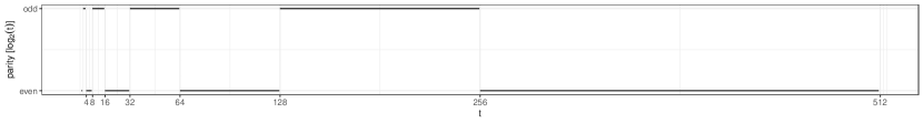
Figure 7: Visualization of the example in Remark 14. Whenever the parity of $\lfloor\log_{2}t\rfloor$ changes from even to odd, the entire mass of $\mathbb{P}_{X_{s}^{t}|\mathbf{H}=\mathbf{h}}$ moves from $(-\infty,-1]^{d}$ to $[1,\infty)^{d}$, and vice versa. In this case, the mixture $\mathbb{P}_{s,\mathbf{h}}^{m}$ in (12) does not converge, and the consistency in Proposition 11 does not hold in general.

Remark 15 (Conditions implying the convergence of mixtures).

We can make the convergence assumption on $\mathbb{P}_{s,\mathbf{h}}^{m}$ more concrete in the case where the distributions in $(\mathbb{P}_{X^{t}_{s}|\mathbf{H}=\mathbf{h}})_{t\in\mathbb{N}}$ differ only in their respective mean vectors. Assume there exist functions $\mu_{s}^{t}:\mathcal{Z}_{\ell}\to\mathbb{R}^{d}$ and $g_{s}:\mathcal{Z}_{\ell}\times\mathbb{R}^{d}\to\mathbb{R}^{d}$, $(s,t)\in\mathbb{R}^{2}\times\mathbb{N}$, and a $d$-dimensional error process $\boldsymbol{\zeta}\mathchoice{\mathrel{\hbox to0.0pt{$\displaystyle\perp$\hss}\mkern 2.0mu{\displaystyle\perp}}}{\mathrel{\hbox to0.0pt{$\textstyle\perp$\hss}\mkern 2.0mu{\textstyle\perp}}}{\mathrel{\hbox to0.0pt{$\scriptstyle\perp$\hss}\mkern 2.0mu{\scriptstyle\perp}}}{\mathrel{\hbox to0.0pt{$\scriptscriptstyle\perp$\hss}\mkern 2.0mu{\scriptscriptstyle\perp}}}\mathbf{H}$, such that for each $s\in\mathbb{R}^{2}$, $\zeta_{s}^{1},\zeta_{s}^{2},\dots$ are i.i.d., and such that for all $(s,t)\in\mathbb{R}^{2}\times\mathbb{N}$ it holds that $X_{s}^{t}=\mu_{s}^{t}(\mathbf{H})+g_{s}(\mathbf{H},\zeta_{s}^{t})$. Assume furthermore that for each $\mathbf{h}\in\mathcal{H}$ and $s\in\mathbb{R}^{2}$, $g_{s}(\mathbf{h},\zeta_{s}^{0})$ has strictly positive density $f_{s,\mathbf{h}}$ w.r.t. the Lebesgue measure on $\mathbb{R}^{d}$. We can then ensure convergence of the mixture distributions $\mathbb{P}_{s,\mathbf{h}}^{m}$ by requiring that for each $\mathbf{h}\in\mathcal{H}$ and $s\in\mathbb{R}^{2}$ there exists some density function $f^{\text{mix}}_{s,\mathbf{h}}$ on $\mathbb{R}^{d}$, such that for all $x\in\mathbb{R}^{d}$ it holds that

$$\lim_{m\to\infty}\frac{1}{m}\sum_{t=1}^{m}\mathbbm{1}_{(-\infty,x]}(\mu_{s}^{t}(\mathbf{h}))=\int_{(-\infty,x]}f^{\text{mix}}_{s,\mathbf{h}}(z)dz.$$

(Intuitively, this equation states that, in the limit $m\to\infty$, the set $\{\mu_{s}^{t}(\mathbf{h})\,:\,t\in\{1,\dots,m\}\}$ looks like an i.i.d. sample drawn from the distribution with density $f^{\text{mix}}_{s,\mathbf{h}}$.) For all $\mathbf{h}\in\mathcal{H}$, $s\in\mathbb{R}^{2}$, $m\in\mathbb{N}$ and $x\in\mathbb{R}^{d}$, we then have

$$\mathbb{P}_{s,\mathbf{h}}^{m}((-\infty,x]) =\frac{1}{m}\sum_{t=1}^{m}\int_{(-\infty,x]}f_{s,\mathbf{h}}(v-\mu_{s}^{t}(\mathbf{h}))dv$$

$$=\int_{\mathbb{R}^{d}}\frac{1}{m}\sum_{t=1}^{m}f_{s,\mathbf{h}}(v-\mu_{s}^{t}(\mathbf{h}))\mathbbm{1}_{(-\infty,x]}(v)dv$$

$$=\int_{\mathbb{R}^{d}}f_{s,\mathbf{h}}(v)\frac{1}{m}\sum_{t=1}^{m}\mathbbm{1}_{(-\infty,x-v]}(\mu_{s}^{t}(\mathbf{h}))dv,$$

and it follows from the dominated convergence theorem that

$$\lim_{m\to\infty}\mathbb{P}_{s,\mathbf{h}}^{m}((-\infty,x]) =\int_{\mathbb{R}^{k}}f_{s,\mathbf{h}}(v)\int_{(-\infty,x-v]}f^{\text{mix}}_{s,\mathbf{h}}(z)dzdv$$

$$=\int_{(-\infty,x]}\int_{\mathbb{R}^{k}}f_{s,\mathbf{h}}(v)f^{\text{mix}}_{s,\mathbf{h}}(z-v)dvdz$$

$$=\int_{(-\infty,x]}(f_{s,\mathbf{h}}\ast f^{\text{mix}}_{s,\mathbf{h}})(z)dz,$$

showing that $\mathbb{P}_{s,\mathbf{h}}^{m}$ converges weakly to the measure with the convoluted density $f_{s,\mathbf{h}}\ast f^{\text{mix}}_{s,\mathbf{h}}$. Since $f_{s,\mathbf{h}}$ is strictly positive, this measure has full support on $\mathbb{R}^{d}$.

Appendix F Simulation experiments

F.1 Observed and unobserved time-varying confounders (synthetic data)

If some of the confounders of $(X_{s}^{t},Y_{s}^{t})$ are not constant across time, the original version of our estimator defined in (5) cannot be expected to be consistent. Given observations from the time-varying confounders, our method can be extended using the approach described in Appendix B.1. We now investigate empirically how the extension can be used, and what happens if the time-varying confounders are ignored. We use a setup similar to Example 7, but where we allow the confounder $\bar{\mathbf{H}}$ to vary across time. Let $\boldsymbol{\zeta},\boldsymbol{\psi},\boldsymbol{\xi}^{t},\boldsymbol{\varepsilon}^{t}$, $t\in\mathbb{N}$, be independent versions of a univariate stationary spatial Gaussian process with mean $0$ and covariance function $u\mapsto e^{-\tfrac{1}{2}\lVert u\rVert_{2}}$. In addition, let $\boldsymbol{\chi}$ be a spatio-temporal process consisting of i.i.d. standard Gaussian random variables. Similarly to Example 7, we define a marginal distribution over $\mathbf{H}=(\bar{\mathbf{H}},\tilde{\mathbf{H}})$ and conditional distributions $\mathbf{X}\,|\,\mathbf{H}$ and $\mathbf{Y}\,|\,(\mathbf{X},\mathbf{H})$ by specifying that for all $(s,t)\in\mathbb{R}^{2}\times\mathbb{N}$,

$$H_{s}^{t} =(\bar{H}_{s}^{t},\tilde{H}_{s}^{t})=(\sigma\cdot\chi_{s}^{t}+a(\sigma)\cdot\zeta_{s},1+b(\sigma)\cdot\zeta_{s}+c(\sigma)\cdot\psi_{s}),$$

$$X_{s}^{t} =\exp(-\lVert s\rVert_{2}^{2}/1000)+(0.2+0.1\cdot\sin(2\pi t/100))\cdot\bar{H}_{s}^{t}\cdot\tilde{H}_{s}^{t}+0.5\cdot\xi_{s}^{t},$$

$$Y_{s}^{t} =(1.5+\bar{H}_{s}^{t}\cdot\tilde{H}_{s}^{t})\cdot X_{s}^{t}+(\bar{H}_{s}^{t})^{2}+\lvert\tilde{H}_{s}^{t}\rvert\cdot\varepsilon_{s}^{t}.$$

Here, $\sigma\in[0,1)$ controls the temporal variation of $\bar{\mathbf{H}}$, and the functions $a(\sigma):=\sqrt{1-\sigma^{2}}$, $b(\sigma):=\frac{1}{2a(\sigma)}$ and $c(\sigma):=\sqrt{1-b(\sigma)^{2}}$ are chosen such that for all $\sigma,s,t$, $\bar{H}_{s}^{t}$ and $\tilde{H}_{s}^{t}$ are standard Gaussian with $\mathbb{E}[\bar{H}_{s}^{t}\cdot\tilde{H}_{s}^{t}]=\frac{1}{2}$. For all $\sigma$, the average causal effect is the linear function $x\mapsto\beta_{0}+\beta_{1}x$, with $\beta_{0}:=\mathbb{E}[(\bar{H}_{0}^{1})^{2}]=1$ and $\beta_{1}:=1.5+\mathbb{E}[\bar{H}_{0}^{1}\cdot\tilde{H}_{0}^{1}]=2$. We consider the same spatial sampling scheme as in Example 7, and generate data sets for a fixed sample size of $m=50$ and $n=1500$. For every data set, we compute an estimate of $\beta_{0}$ and $\beta_{1}$ using an estimator of the form (10), which uses data from $\bar{\mathbf{H}}$ to adjust for both observed time-varying confounding and unobserved time-invariant confounding using the procedure described in Appendix B.1. (For the step where $Y_{s}^{t}$ is regressed onto $(X_{s}^{t},\bar{H}_{s}^{t})$, we assume a linear regression model which includes only the additive terms $X_{s}^{t}$, $X_{s}^{t}\cdot\bar{H}_{s}^{t}$ and $(\bar{H}_{s}^{t})^{2}$, and no intercept.) For comparison, we also show results for the original estimator (7) which assumes that all confounders are time-invariant, and from a classical linear regression which ignores the existence of confounders altogether. The results are shown in Figure 8. If $\sigma^{2}=0$, that is, all confounders are time-invariant, our procedure (‘LSCM’) correctly estimates $\beta_{0}$ and $\beta_{1}$. As the variance $\sigma^{2}$ of the temporally varying term of $H_{s}^{t}$ increases, our procedure becomes slightly biased, but still gives better results than ignoring the confounders (‘no adjustm.’). The extension of our method (‘LSCM + Hbar’), which assumes that $\bar{H}_{s}^{t}$ is observed, is empirically unbiased in all scenarios.

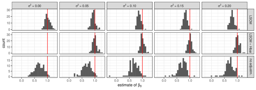
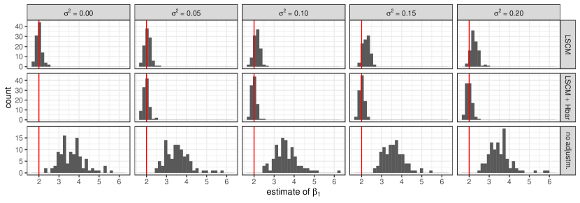
Figure 8: Estimates of $\beta_{0}$ (top) and $\beta_{1}$ (bottom) for the simulation experiment described in Appendix F.1. The true values ($\beta_{0}=1$ and $\beta_{1}=2$) are indicated by vertical red lines. If all confounders are time-invariant ($\sigma^{2}=0$), our procedure (‘LSCM’) correctly estimates the causal parameters. As the temporal variation of the confounder $\bar{H}_{s}^{t}$ increases (that is, as $\sigma^{2}$ becomes larger), our procedure becomes biased. If $\bar{H}_{s}^{t}$ is observed, it can readily be integrated into our method, see Appendix B.1. In this example, the resulting procedure (‘LSCM + Hbar’) yields empirically unbiased estimators. For $\sigma^{2}=0$, this method is undefined, since the location-wise regression of $Y_{s}^{t}$ onto $(X_{s}^{t},H_{s}^{t})$ is not identified.

F.2 Generating semi-real data

We conduct two semi-real experiments to assess the performance of our methodology for the specific data application introduced in Section 4. We use the original data for conflict $\mathbf{X}$, and generate new responses $\tilde{\mathbf{Y}}$ using the following approach. For different values of $\beta\in\mathbb{R}$, we generate, for every $s,t$, a new response $\tilde{Y}_{s}^{t}$ from the equation

$$\tilde{Y}_{s}^{t}:=\beta X_{s}^{t}+\tilde{\varepsilon}_{s}^{t}.$$ (13)

Here, the noise variable $\tilde{\varepsilon}_{s}^{t}$ is drawn from the empirical forest loss distribution at location $s$. More precisely, the variables in $\tilde{\boldsymbol{\varepsilon}}=(\tilde{\varepsilon}_{s}^{t})_{(s,t)\in\{s_{1},\dots,s_{n}\}\times\{1,\dots,m\}}$ are conditionally independent given $\mathbf{Y}$ and have (conditional) marginal distributions $\tilde{\varepsilon}_{s}^{t}\,|\,\mathbf{Y}=\mathbf{y}\sim\text{Uniform}(\{y_{s}^{1},\dots,y_{s}^{m}\})$. It is worth noting that the variables in $\tilde{\boldsymbol{\varepsilon}}$ do not correspond to classical independent error terms in a regression model: they do not have mean zero ($\mathbf{Y}$ has positive support), they are not mutually independent (they inherit all time-invariant spatial dependence in $\mathbf{Y}$), and they are not independent of the other variables in the regression equation (roughly speaking, the dependence between $\tilde{\boldsymbol{\varepsilon}}$ and $\mathbf{X}$ amounts to the dependence between $\mathbf{Y}$ and $\mathbf{X}$ that is induced via all time-invariant confounders). Consequently, semi-synthetic datasets $(\mathbf{X},\tilde{\mathbf{Y}})$ generated from the above model share the same time-invariant confounding as the original data. The true causal effect of $\mathbf{X}$ on $\tilde{\mathbf{Y}}$ is $T=f_{\text{AVE}(X\to Y)}(1)-f_{\text{AVE}(X\to Y)}(0)=\beta$.

F.3 Power analysis (semi-real data)

Using the data generating process from Section F.2, we generate, for each $\beta$ in the set $\{0,0.02,0.04,0.06,0.08\}$, 100 independent responses $\tilde{\mathbf{Y}}_{\beta}^{(1)},\dots,\tilde{\mathbf{Y}}_{\beta}^{(100)}$ from (13). For each resulting data set $(\mathbf{X},\tilde{\mathbf{Y}}_{\beta}^{(i)})$, we compute a $p$-value for the hypothesis $H_{0}$ of a vanishing causal effect using the resampling test introduced in Section 3. For comparison, we also include results for the two alternative testing procedures described in Section 4.3, which assume that there is no confounder, or that the only confounder is the distance to the closest road ($\mathbf{W}$), respectively (see also Figure 4, where we compare these three methods on the original data). In addition, we use a standard two-sample $t$-test, which tests whether $\mathbb{E}[Y_{s}^{t}\,|\,X_{s}^{t}=1]=\mathbb{E}[Y_{s}^{t}\,|\,X_{s}^{t}=0]$ (regarded as a test of the causal hypothesis $H_{0}$, this test assumes that there are no confounders). For each $\beta$ and each testing procedure, we compute the number of rejections of $H_{0}$ (out of $100$) at level $\alpha=0.05$. The results are shown in Figure 9.

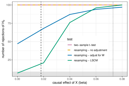
Figure 9: Results of the power analysis described in Appendix F.3. The colored curves show the empirial power of the different methods. For increasing strength of the causal effect $\beta$, all tests tend to reject $H_{0}$. The vertical lines correspond to the absolute values of the estimated causal effect on the real data using our estimator (dashed), and the naive estimator based on difference in sample averages (dotted). If, indeed, the true causal effect was as large as suggested by the naive analysis, our method (green curve) would detect it with high certainty. While the alternative procedures obtain higher detection rates, our method is the only one which holds the correct test level $\alpha=0.05$: for $\beta=0$, only the green curve takes a value that lies within the lower $95\%$-quantile range of a $\text{Bin}(100,\alpha)$-distribution (grey area).

As $\beta$ increases, our testing procedure (green curve) tends to reject $H_{0}$ more often. For simulated data sets where the true causal effect is of the same magnitude as the estimated causal effect on the original data ($T=-0.018$, the absolute value of which is shown by a vertical dashed line), we reject in roughly $20\%$ of the cases. If the true effect is as large as suggested by the difference in sample averages on the original data ($T=0.073$, dotted vertical line), our test almost always rejects $H_{0}$. While the alternative approaches obtain higher rejection rates, none of them is able to keep the desired test level $\alpha=0.05$ (see Figure 9).

F.4 Bias due to a reduced sample size (semi-real data)

The estimator (8) is constructed from a reduced dataset. The used data exclusion criterion is not independent of the assumed hidden confounders (i.e., the distribution of the hidden variables is expected to differ between the reduced data and the original data), and therefore potentially results in a biased estimator. Under additional assumptions on the underlying LSCM, however, (8) may still be used to estimate $T$. Below, we first give a population version argument, and then verify this argument empirically using a simulation experiment.

Assume that there is no interaction between $X_{s}^{t}$ and $H_{s}^{t}$ in the causal mechanism for $Y_{s}^{t}$, i.e., the function $f$ in (2) splits into $f_{1}(X_{s}^{t},\varepsilon_{s}^{t})+f_{2}(H_{s}^{t},\varepsilon_{s}^{t})$. Then, the conditional expectation of $Y_{s}^{t}\,|\,(X_{s}^{t},H_{s}^{t})$ likewise splits additively into a function of $X_{s}^{t}$ and a function of $H_{s}^{t}$. Using Proposition 5, it follows that any two different models for the marginal distribution of the latent process $\mathbf{H}$ induce average causal effects $f_{\text{AVE}(X\to Y)}$ that are equal up to an additive constant. In particular, every model for $\mathbf{H}$ induces the same value for $T$. By regarding the reduced dataset as a realization from a modified LSCM, in which the distribution of $\mathbf{H}$ has been altered, this argument justifies the use of (8) as an estimator for $T$.

We now investigate the above statement empirically. To do so, we generate responses $\tilde{Y}_{s}^{t}$ from the model (13) in Section F.2, but where we additionally include the additive term $\alpha\log W_{s}^{t}$, where $\mathbf{W}$ corresponds to the observed realization of the distance-to-road variable. Due to the highly skewed distribution of $\mathbf{W}$, we model its influence on $\tilde{Y}_{s}^{t}$ on a log-scale. For datasets generated in this way, the causal effect of $X_{s}^{t}$ on $\tilde{Y}_{s}^{t}$ is confounded both by the dependence induced by $\tilde{\varepsilon}_{s}^{t}$ (which includes all time-invariant confounding present in the original data), and by the dependence induced by the term $\alpha\log W_{s}^{t}$. For varying values of $\alpha$ and $\beta$, we simulate $100$ indendent responses $\tilde{\mathbf{Y}}_{\alpha,\beta}^{(1)},\dots,\tilde{\mathbf{Y}}_{\alpha,\beta}^{(100)}$. On each dataset $(\mathbf{X},\tilde{\mathbf{Y}}_{\alpha,\beta}^{(i)})$, we compute an estimate of the causal effect $T=\beta$ using our estimator (8). For comparison, we also include the two alternative estimators introduced in Section 4.3, which assume that there is no confounder, or that the only confounder is $\mathbf{W}$, respectively (see also Figure 2, where we compare these three methods on the original data). For each choice of $\alpha,\beta$, and each method, we obtain an estimate of the bias $\mathbb{E}[\hat{T}]-T$. The results are shown in Figure 10.

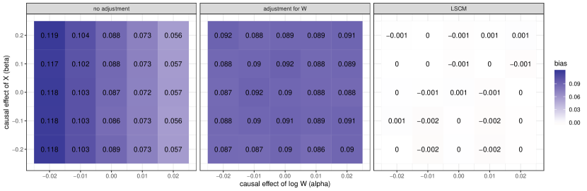
Figure 10: Results of the bias analysis described in Appendix F.4. Along the first axis, we vary the causal effect of $\log W_{s}^{t}$; along the second axis that of $X_{s}^{t}$. For each parameter setting and each method, we compute an estimate $\hat{\mathbb{E}}[\hat{T}]-T$ of the bias, which is shown as numbers and color coding. In these experiments, the causal effect of $X_{s}^{t}$ on $Y_{s}^{t}$ is confounded both by the observed variable $W_{s}^{t}$ and by unobserved time-invariant confounders (whose influence is transmitted via the error term $\tilde{\varepsilon}_{s}^{t}$). The approach which does not adjust for confounding (left), and the approach which only adjusts for $W_{s}^{t}$ (middle), therefore lead to biased estimators. Our estimator (right) is approximately unbiased in all parameter settings. This property relies on the fact that, in the structural equations for $Y_{s}^{t}$, there is no interaction between $X_{s}^{t}$ and any of the confounders.

Both alternative approaches lead to biased estimators, since they either do not adjust for confounding, or only adjust for one of the confounders. Interestingly, the estimator shown in the left-most panel becomes less biased as the causal effect of $\log W_{s}^{t}$ increases. An explanation for this could be the following. We hypothesize that most time-invariant confounders introduce a positive correlation between $X_{s}^{t}$ and $Y_{s}^{t}$ (e.g., for a large distance to the closest road or for a small population density, both $X_{s}^{t}$ and $Y_{s}^{t}$ tend to take small values). As argued in Appendix F.2, this dependence is preserved by our simulation procedure, and therefore confounds the causal effect of $X_{s}^{t}$ on $\tilde{Y}_{s}^{t}$ positively. At the same time, the term $\alpha\log W_{s}^{t}$ introduces additional confounding correlation between $X_{s}^{t}$ and $\tilde{Y}_{s}^{t}$. For $\alpha<0$, the additionally introduced correlation is positive (because we expect $W_{s}^{t}$ and $X_{s}^{t}$ to be negatively correlated), and therefore adds to the overall confounding. For $\alpha>0$, it is negative, and hence cancels out with some of the confounding introduced by $\tilde{\varepsilon}_{s}^{t}$. After adjusting for $W_{s}^{t}$, the confounding reduces to what is induced by $\tilde{\varepsilon}_{s}^{t}$ (indeed, the bias in the middle panel roughly coincides with the bias in the left panel for $\alpha=0$). In all settings, our estimator (right panel) is approximately unbiased.

Appendix G Further results on resampling tests

G.1 Temporal autocorrelation in the response variable

A central assumption of the LSCM model class is that the error process of $\mathbf{Y}$ is independent over time. This assumption says that all dependencies between different temporal instances of $\mathbf{Y}$ are induced via the covariates $\mathbf{X}$ or the time-invariant confounders $\mathbf{H}$. In practice, there may be other time-varying conditions influencing forest loss, thereby inducing a temporal dependence in $\mathbf{Y}$ which cannot be explained by $(\mathbf{X},\mathbf{H})$. In this case, the exchangeability property in Proposition 8, and therefore the level of our resampling test, is violated. To incorporate temporal autocorrelation in the response variable, we adopt a block-permutation scheme: we divide the period 2000–2018 into 6 blocks (2000–2002, 2003–2005, …, 2016–2018), and perform a block-wise permutation of the data from $\mathbf{Y}$. This procedure leaves the within-block dependence structure in $\mathbf{Y}$ intact. The results align with our previous findings: $P=0.892$ for the test of an instantaneous effect, and $P=0.498$ for the test of a temporally lagged effect (when using the same test statistics as in Section 4.4).

G.2 Spatial block-permutation scheme for Model 1

In Section 4.3, we describe alternative permutation schemes to test the null hypotheses in Models 1 and 2. Strictly speaking, we require additional exchangeability assumptions on $\mathbf{Y}$ to ensure the validity of the corresponding resampling tests. Here, we investigate an alternative permutation scheme for Model 1. To account for the spatial autocorrelation in $\mathbf{Y}$, we adopt a spatial block-permutation: for every year 2000–2018, observations are grouped into blocks of size $100$\mathrm{km}$\times 100$\mathrm{km}$$. To obtain resampled datasets, we then permute values of $\mathbf{Y}$ in these blocks of data, thereby leaving the spatial dependence within each block intact. Observations which do not fall in any of the blocks are permuted randomly.

Figure 11: Block structure for the spatial permutation scheme (left) and results of resampling tests (right) for the null hypothesis in Model 1 from Section 4.4. The test statistic $\hat{T}=\hat{f}^{nm}_{\text{AVE}(X\to Y)}(1)-\hat{f}^{nm}_{\text{AVE}(X\to Y)}(0)$ is indicated by a red vertical bar. The empirical distribution of the test statistic under this permutation scheme (top right) has a higher variance than under the permutation scheme used in Section 4.4 (bottom right), resulting in a slightly larger $p$-value of $0.008$ compared with the $p$-value of $0.002$ for the original test. The significance of the test does not change.

As seen in Figure 11, this procedure slightly increases the $p$-value, but does not affect the significance of the test.

Appendix H Proofs

H.1 Proof of Proposition 4

By definition, intervening on $\mathbf{X}$ leaves the conditional distribution $\mathbf{Y}\,|\,(\mathbf{X},\mathbf{H})$ unchanged. Under $\mathbb{P}_{x}$, the property (2) therefore still holds for the same error process $\boldsymbol{\varepsilon}$. Since also the marginal distribution of $\mathbf{H}$ is unaffected by the intervention, we have that

$$\mathbb{E}_{\mathbb{P}_{x}}[Y_{s}^{t}] =\mathbb{E}_{\mathbb{P}_{x}}[f(X_{s}^{t},H^{t}_{s},\varepsilon_{s}^{t})]=\mathbb{E}_{\mathbb{P}_{x}}[f(x,H^{t}_{s},\varepsilon_{s}^{t})]$$

$$=\mathbb{E}[f(x,H^{t}_{s},\varepsilon_{s}^{t})]=\mathbb{E}[f(x,H^{1}_{0},\varepsilon_{0}^{1})]=f_{\text{AVE}(X\to Y)}(x),$$

as desired. $\hfill\square$

H.2 Proof of Theorem 6

Consider a fixed $x\in\mathcal{X}$. For every $n,m\in\mathbb{N}$ we have that

$$\hat{f}^{nm}_{\text{AVE}(X\rightarrow Y)}(\mathbf{X}_{n}^{m},\mathbf{Y}_{n}^{m})(x)-f_{\text{AVE}(X\rightarrow Y)}(x) =\frac{1}{n}\sum_{i=1}^{n}\hat{f}^{m}_{Y|X}(\mathbf{X}_{s_{i}}^{m},\mathbf{Y}_{s_{i}}^{m})(x)-\mathbb{E}\left[f_{Y|(X,H)}(x,H_{0}^{1})\right]$$

$$=\frac{1}{n}\sum_{i=1}^{n}\left(\hat{f}^{m}_{Y|X}(\mathbf{X}_{s_{i}}^{m},\mathbf{Y}_{s_{i}}^{m})(x)-f_{Y|(X,H)}(x,H^{1}_{s_{i}})\right)$$

$$\quad+\frac{1}{n}\sum_{i=1}^{n}f_{Y|(X,H)}(x,H^{1}_{s_{i}})-\mathbb{E}\left[f_{Y|(X,H)}(x,H_{0}^{1})\right]$$

$$=r_{1}(\mathbf{X}_{n}^{m},\mathbf{Y}_{n}^{m},\mathbf{H}_{n}^{1})+r_{2}(\mathbf{H}_{n}^{1}),$$

where

$$r_{1}(\mathbf{X}_{n}^{m},\mathbf{Y}_{n}^{m},\mathbf{H}_{n}^{1}) :=\frac{1}{n}\sum_{i=1}^{n}\left(\hat{f}^{m}_{Y|X}(\mathbf{X}_{s_{i}}^{m},\mathbf{Y}_{s_{i}}^{m})(x)-f_{Y|(X,H)}(x,H^{1}_{s_{i}})\right)\text{ and }$$

$$r_{2}(\mathbf{H}_{n}^{1}) :=\frac{1}{n}\sum_{i=1}^{n}f_{Y|(X,H)}(x,H^{1}_{s_{i}})-\mathbb{E}\left[f_{Y|(X,H)}(x,H_{0}^{1})\right].$$

It follows that for any $\delta>0$,

$$\mathbb{P}\left(\left|\hat{f}^{nm}_{\text{AVE}(X\rightarrow Y)}(\mathbf{X}_{n}^{m},\mathbf{Y}_{n}^{m})(x)-f^{0}_{\text{AVE}(X\rightarrow Y)}(x)\right|>\delta\right) \leq\mathbb{P}\left(|r_{1}(\mathbf{X}_{n}^{m},\mathbf{Y}_{n}^{m},\mathbf{H}_{n}^{1})|>\delta/2\right)$$

$$\quad+\mathbb{P}\left(|r_{2}(\mathbf{H}_{n}^{1})|>\delta/2\right).$$

Let now $\alpha>0$ be arbitrary. By Assumption A1, there exists $N\in\mathbb{N}$ such that for all $n\geq N$, $\mathbb{P}(\lvert r_{2}(\mathbf{H}_{n}^{1})\rvert\geq\delta/2)\leq\alpha/2$. By Assumption A2, we can for any such $n\geq N$ find $M_{n}\in\mathbb{N}$, such that for all $i=1,\dots,n$ and all $m\geq M_{n}$ it holds that $\mathbb{P}(\lvert\hat{f}^{m}_{Y|X}(\mathbf{X}_{s_{i}}^{m},\mathbf{Y}_{s_{i}}^{m})(x)-f_{Y|(X,H)}(x,H^{1}_{s_{i}})\rvert>\delta/2)\leq\alpha/(2n)$. For all $m\geq M_{n}$ we then have

$$\mathbb{P}\left(\lvert r_{1}(\mathbf{X}_{n}^{m},\mathbf{Y}_{n}^{m},\mathbf{H}_{n}^{1})\rvert>\delta/2\right) \leq\mathbb{P}\left(\frac{1}{n}\sum_{i=1}^{n}\left|\hat{f}^{m}_{Y|X}(\mathbf{X}_{s_{i}}^{m},\mathbf{Y}_{s_{i}}^{m})(x)-f_{Y|(X,H)}(x,H^{1}_{s_{i}})\right|>\delta/2\right)$$

$$\leq\mathbb{P}\left(\bigcup_{i=1}^{n}\left\{\left|\hat{f}^{m}_{Y|X}(\mathbf{X}_{s_{i}}^{m},\mathbf{Y}_{s_{i}}^{m})(x)-f_{Y|(X,H)}(x,H^{1}_{s_{i}})\right|>\delta/2\right\}\right)$$

$$\leq\sum_{i=1}^{n}\mathbb{P}\left(\left|\hat{f}^{m}_{Y|X}(\mathbf{X}_{s_{i}}^{m},\mathbf{Y}_{s_{i}}^{m})(x)-f_{Y|(X,H)}(x,H^{1}_{s_{i}})\right|>\delta/2\right)$$

$$\leq\sum_{i=1}^{n}\alpha/(2n)=\alpha/2,$$

and the result follows. $\hfill\square$

H.3 Proof of Proposition 10

By construction, $(H^{1}_{s_{n}})_{n\in\mathbb{N}}$ can be decomposed into $m$ subsequences $(H^{1}_{s_{(n-1)m+j}})_{n\in\mathbb{N}}$, $j\in\{1,\dots,m\}$, each of which corresponds to an equally spaced sampling of $\mathbf{H}^{1}$ along the first spatial axis. We fist prove that each of these subsequences satisfies Assumption A1, and then conclude that the same must hold for the original sequence $(H^{1}_{s_{n}})_{n\in\mathbb{N}}$. Let $j\in\{1,\dots,m\}$ and let $\varphi:\mathbb{R}^{\ell}\to\mathbb{R}$ be a measurable function with $\mathbb{E}[\lvert\varphi(H_{0}^{1})\rvert]<\infty$. For notational simplicity, let for each $n\in\mathbb{N}$, $Z_{n}:=H^{1}_{s_{(n-1)m+j}}$. The idea is to apply an ergodic theorem for real-valued stationary and ergodic time series [e.g., Rønn-Nielsen and Sokol, 2013, Corollary 2.3.13] to the sequence $(\varphi(Z_{n}))_{n\in\mathbb{N}}$. By stationarity of the process $\mathbf{H}^{1}$, and by choice of the sampling scheme, $(\varphi(Z_{n}))_{n\in\mathbb{N}}$ is indeed stationary. We need to show that $(\varphi(Z_{n}))_{n\in\mathbb{N}}$ is also ergodic. Using [Rønn-Nielsen and Sokol, 2013, Lemma 2.3.15], this follows by proving the following mixing condition: for all $p,q\geq 1$ and all $A_{1},\dots,A_{p}\in\mathcal{B}(\mathbb{R})$ and $B_{1},\dots,B_{q}\in\mathcal{B}(\mathbb{R})$, it holds that

$$\begin{split}&\mathbb{P}(\varphi(Z_{1})\in A_{1},\dots,\varphi(Z_{p})\in A_{p},\varphi(Z_{n+1})\in B_{1},\dots,\varphi(Z_{n+q})\in B_{q})\\ \to\;&\mathbb{P}(\varphi(Z_{1})\in A_{1},\dots,\varphi(Z_{p})\in A_{p})\cdot\mathbb{P}(\varphi(Z_{1})\in B_{1},\dots,\varphi(Z_{q})\in B_{q})\quad\text{ as }n\to\infty.\end{split}$$ (14)

Since the finite-dimensional distributions of $(Z_{n})_{n\in\mathbb{N}}$ are Gaussian, this condition is easily verified. Let $p,q\geq 1$, and let $\mathbb{P}_{1}=\mathcal{N}(\mu_{1},\Sigma_{1})$ and $\mathbb{P}_{2}=\mathcal{N}(\mu_{2},\Sigma_{2})$ be the distributions of $(Z_{1},\dots,Z_{p})$ and $(Z_{1},\dots,Z_{q})$, respectively. Property (14) follows if we can show that $(Z_{1},\dots,Z_{m},Z_{n+1},\dots,Z_{n+p})$ converges to $\mathbb{P}_{1}\otimes\mathbb{P}_{2}=\mathcal{N}((\mu_{1},\mu_{2}),\text{diag}(\Sigma_{1},\Sigma_{2}))$ in distribution as $n\to\infty$. Convergence of the mean vector is trivial, and convergence of the covariance matrix follows by the assumption on $C$ and our choice of spatial sampling (the distance between the respective locations at which $(Z_{1},\dots,Z_{m})$ and $(Z_{n+1},\dots,Z_{n+p})$ are observed tends to infinity as $n$ increases). To prove that the limit distribution is indeed Gaussian, one can then consider characteristic functions and apply a combination of Levy’s Continuity Theorem [e.g., Williams, 1991, Theorem 18.1] and the Cramér-Wold Theorem [Cramér and Wold, 1936]. This proves that $\frac{1}{n}\sum_{i=1}^{n}\varphi(Z_{i})\to\mathbb{E}[\varphi(Z_{1})]$ in probability as $n\to\infty$, i.e., the subsequence $(H^{1}_{s_{(n-1)m+j}})_{n\in\mathbb{N}}$ satisfies Assumption A1. Since $j$ was arbitrary, this holds true for all $j\in\{1,\dots,m\}$. It remains to prove that also the original sequence $(H^{1}_{s_{n}})_{n\in\mathbb{N}}$ satisfies Assumption A1.

Let an integrable function $\varphi:\mathbb{R}^{\ell}\to\mathbb{R}$ be given, and assume first that $\mathbb{E}[\varphi(H_{0}^{1})]=0$. For every $j\in\{1,\dots,m\}$ and $i\in\mathbb{N}$, define $S_{i}^{j}:=\sum_{k=1}^{i}\varphi(H^{1}_{s_{(k-1)m+j}})$. By the first part of the proof, we have that for all $j$, $\tfrac{1}{i}S_{i}^{j}\to 0$ in probability as $i\to\infty$. We want to show that also $\tfrac{1}{n}\sum_{k=1}^{n}\varphi(H^{1}_{s_{k}})\to 0$ in probability as $n\to\infty$. Let $\delta,\alpha>0$ and choose $I\in\mathbb{N}$ such that for all $j\in\{1,\dots,m\}$ and $i\geq I$, $\mathbb{P}(\frac{1}{i}\lvert S_{i}^{j}\rvert>\delta/m)\leq\alpha/m$. Define $N:=mI+1$ and pick an arbitrary $n\geq N$. We can then write $n=im+j$ for some $i\geq I$ and $j\in\{1,\dots,m\}$. With $J_{1}:=\{1,\dots,j\}$ and $J_{2}=\{1,\dots,m\}\setminus J_{1}$, we then have

$$\mathbb{P}(\frac{1}{n}|\sum_{k=1}^{n}\varphi(H^{1}_{s_{k}})|>\delta) =\mathbb{P}(\frac{1}{n}|\sum_{{j^{\prime}}\in J_{1}}S_{i+1}^{j^{\prime}}+\sum_{{j^{\prime}}\in J_{2}}S_{i}^{{j^{\prime}}}|>\delta)$$

$$\leq\mathbb{P}(\sum_{{j^{\prime}}\in J_{1}}\frac{1}{i+1}\lvert S_{i+1}^{j^{\prime}}\rvert+\sum_{{j^{\prime}}\in J_{2}}\frac{1}{i}\lvert S_{i}^{j^{\prime}}\rvert>\delta)$$

$$\leq\sum_{{j^{\prime}}\in J_{1}}\mathbb{P}(\frac{1}{i+1}\lvert S_{i+1}^{j^{\prime}}\rvert>\delta/m)+\sum_{{j^{\prime}}\in J_{2}}\mathbb{P}(\frac{1}{i}\lvert S_{i}^{j^{\prime}}\rvert>\delta/m)\leq\alpha,$$

which completes the proof in the case where $\mathbb{E}[\varphi(H_{0}^{1})]=0$. The general case follows by applying the above result to the function $\tilde{\varphi}=\varphi-\mathbb{E}[\varphi(H_{0}^{1})]$. $\square$

H.4 Proof of Proposition 11

Let $s\in\mathbb{R}^{2}$ and $\mathbf{h}\in\mathcal{H}$. With $\gamma_{s}:=f_{1}(h_{s}^{1})$, it follows from (L1) that for all $x$ and $t$, we have $\mathbb{E}[Y_{s}^{t}\,|\,X_{s}^{t}=x,H_{s}^{t}=h_{s}^{t}]=\varphi(x)^{\top}\gamma_{s}$. It therefore suffices to prove that $\hat{\gamma}_{s}^{m}\to\gamma_{s}$ in probability under $\mathbb{P}_{\mathbf{h}}$. For the ease of notation, we omit all sub- and superscripts from $\mathbf{Y}_{s}^{m},\mathbf{\Phi}_{s}^{m}$ and $\boldsymbol{\xi}_{s}^{m}$ in the below calculations. Let $c>0$ be such that (L3) holds true and let $\delta>0$ be arbitrary. For every $m\in\mathbb{N}$, we then have

$$\mathbb{P}_{\mathbf{h}}(\lVert\gamma_{s}-\hat{\gamma}_{s}^{m}\rVert_{2}>\delta) =\mathbb{P}_{\mathbf{h}}(\lVert\gamma_{s}-(\mathbf{\Phi}^{\top}\mathbf{\Phi})^{-1}\mathbf{\Phi}^{\top}\mathbf{Y}\rVert_{2}>\delta)$$

$$=\mathbb{P}_{\mathbf{h}}(\lVert\gamma_{s}-(\mathbf{\Phi}^{\top}\mathbf{\Phi})^{-1}\mathbf{\Phi}^{\top}(\mathbf{\Phi}\gamma_{s}+\boldsymbol{\xi})\rVert_{2}>\delta)$$

$$=\mathbb{P}_{\mathbf{h}}(\lVert(\mathbf{\Phi}^{\top}\mathbf{\Phi})^{-1}\mathbf{\Phi}^{\top}\boldsymbol{\xi}\rVert_{2}>\delta)$$

$$\leq\mathbb{P}_{\mathbf{h}}(\lVert(\tfrac{1}{m}\mathbf{\Phi}^{\top}\mathbf{\Phi})^{-1}\rVert_{2}\lVert\tfrac{1}{m}\mathbf{\Phi}^{\top}\boldsymbol{\xi}\rVert_{2}>\delta\,|\,)$$

$$=\mathbb{P}_{\mathbf{h}}((\lambda_{\text{min}}(\tfrac{1}{m}\mathbf{\Phi}^{\top}\mathbf{\Phi}))^{-1}\lVert\tfrac{1}{m}\mathbf{\Phi}^{\top}\boldsymbol{\xi}\rVert_{2}>\delta)$$

$$=\mathbb{P}_{\mathbf{h}}((\lambda_{\text{min}}(\tfrac{1}{m}\mathbf{\Phi}^{\top}\mathbf{\Phi}))^{-1}\lVert\tfrac{1}{m}\mathbf{\Phi}^{\top}\boldsymbol{\xi}\rVert_{2}>\delta\text{ and }\lambda_{\text{min}}\left(\tfrac{1}{m}\mathbf{\Phi}^{\top}\mathbf{\Phi}\right)>c)$$

$$\quad+\mathbb{P}_{\mathbf{h}}((\lambda_{\text{min}}(\tfrac{1}{m}\mathbf{\Phi}^{\top}\mathbf{\Phi}))^{-1}\lVert\tfrac{1}{m}\mathbf{\Phi}^{\top}\boldsymbol{\xi}\rVert_{2}>\delta\text{ and }\lambda_{\text{min}}\left(\tfrac{1}{m}\mathbf{\Phi}^{\top}\mathbf{\Phi}\right)\leq c)$$

$$\leq\mathbb{P}_{\mathbf{h}}(\lVert\tfrac{1}{m}\mathbf{\Phi}^{\top}\boldsymbol{\xi}\rVert_{2}>c\delta)+\mathbb{P}_{\mathbf{h}}(\lambda_{\text{min}}\left(\tfrac{1}{m}\mathbf{\Phi}^{\top}\mathbf{\Phi}\right)\leq c),$$

which tends to zero as $m\to\infty$ by (L2) and (L3). $\square$

H.5 Proof of Proposition 8

Recall our definition of $\mathcal{H}\subseteq\mathcal{Z}_{\ell}$ as the set of functions $\mathbf{h}:\mathbb{R}^{2}\times\mathbb{N}\to\mathbb{R}^{\ell}$ that are constant in the time-argument. Since $\mathbf{H}$ is time-invariant, we have that $\mathbb{P}(\mathbf{H}\in\mathcal{H})=1$. It therefore suffices to prove that for all $\mathbf{h}\in\mathcal{H}$, $(\mathbf{X}_{n}^{m},\sigma(\mathbf{Y}_{n}^{m}))\stackrel{{\scriptstyle d}}{{=}}(\mathbf{X}_{n}^{m},\mathbf{Y}_{n}^{m})$ under $\mathbb{P}(\,\cdot\,|\,\mathbf{H}=\mathbf{h})$. Assume that $H_{0}$ holds true, and let $\sigma$ be a permutation of $\{1,\dots,m\}$. Then, there exists a function $\tilde{f}:\mathbb{R}^{\ell+1}\to\mathbb{R}$ and an error process $\boldsymbol{\varepsilon}\mathchoice{\mathrel{\hbox to0.0pt{$\displaystyle\perp$\hss}\mkern 2.0mu{\displaystyle\perp}}}{\mathrel{\hbox to0.0pt{$\textstyle\perp$\hss}\mkern 2.0mu{\textstyle\perp}}}{\mathrel{\hbox to0.0pt{$\scriptstyle\perp$\hss}\mkern 2.0mu{\scriptstyle\perp}}}{\mathrel{\hbox to0.0pt{$\scriptscriptstyle\perp$\hss}\mkern 2.0mu{\scriptscriptstyle\perp}}}(\mathbf{X},\mathbf{H})$ such that for all $(s,t)\in\mathbb{R}^{2}\times\mathbb{N}$, $Y_{s}^{t}=\tilde{f}(H_{s},\varepsilon_{s}^{t})$. It follows that the conditional distribution of $\mathbf{Y}\,|\,(\mathbf{X},\mathbf{H})$ does not depend on $\mathbf{X}$, and hence that $\mathbf{X}$ and $\mathbf{Y}$ are conditionally independent given $\mathbf{H}$. Furthermore, since $\boldsymbol{\varepsilon}^{1},\boldsymbol{\varepsilon}^{2},\dots$ are i.i.d., we have that for all $\mathbf{h}\in\mathcal{H}$, $\mathbf{Y}^{1},\dots,\mathbf{Y}^{m}$ are i.i.d. under $\mathbb{P}(\,\cdot\,|\,\mathbf{H}=\mathbf{h})$. For all $\mathbf{h}\in\mathcal{H}$, it therefore holds that $(\mathbf{X}_{n}^{m},\sigma(\mathbf{Y}_{n}^{m}))\stackrel{{\scriptstyle d}}{{=}}(\mathbf{X}_{n}^{m},\mathbf{Y}_{n}^{m})$ under $\mathbb{P}(\,\cdot\,|\,\mathbf{H}=\mathbf{h})$, and the result follows. $\hfill\square$

References

- Angelsen and Kaimowitz [1999] A. Angelsen and D. Kaimowitz. Rethinking the causes of deforestation: lessons from economic models. The world bank research observer, 14(1):73–98, 1999.
- Avitabile et al. [2016] V. Avitabile, M. Herold, G. B. M. Heuvelink, S. L. Lewis, O. L. Phillips, G. P. Asner, et al. An integrated pan-tropical biomass map using multiple reference datasets. Global change biology, 22(4):1406–1420, 2016.
- Baumann and Kuemmerle [2016] M. Baumann and T. Kuemmerle. The impacts of warfare and armed conflict on land systems. Journal of land use science, 11(6):672–688, 2016.
- Bertolacci et al. [2019] M. Bertolacci, E. Cripps, et al. Climate inference on daily rainfall across the Australian continent, 1876–2015. The Annals of Applied Statistics, 13(2):683–712, 2019.
- Bollen [2014] K. A. Bollen. Structural equations with latent variables. John Wiley & Sons, 2014.
- Butsic et al. [2015] V. Butsic, M. Baumann, A. Shortland, S. Walker, and T. Kuemmerle. Conservation and conflict in the Democratic Republic of Congo: The impacts of warfare, mining, and protected areas on deforestation. Biological conservation, 191:266–273, 2015.
- Castro-Nunez et al. [2017] A. Castro-Nunez, O. Mertz, A. Buritica, C. C. Sosa, and S. T. Lee. Land related grievances shape tropical forest-cover in areas affected by armed-conflict. Applied Geography, 85:39–50, 2017.
- Chaplain et al. [1999] M. A. J. Chaplain, G. D. Singh, and J. C. McLachlan. On growth and form: spatio-temporal pattern formation in biology. Wiley, 1999.
- Clerici et al. [2020] N. Clerici, D. Armenteras, P. Kareiva, R. Botero, J. P. Ramírez-Delgado, G. Forero-Medina, et al. Deforestation in Colombian protected areas increased during post-conflict periods. Scientific Reports, 10(1):1–10, 2020.
- Collier et al. [2000] P. Collier et al. Economic causes of civil conflict and their implications for policy. Technical Report 76632, The World Bank, Washington, D.C., United States, 2000.
- Cramér and Wold [1936] H. Cramér and H. Wold. Some theorems on distribution functions. Journal of the London Mathematical Society, 1(4):290–294, 1936.
- Cressie and Wikle [2015] N. Cressie and C. K. Wikle. Statistics for spatio-temporal data. John Wiley & Sons, 2015.
- Croicu and Sundberg [2015] M. Croicu and R. Sundberg. UCDP georeferenced event dataset codebook version 4.0. Journal of Peace Research, 50(4):523–532, 2015.
- Dávalos et al. [2016] L. M. Dávalos, K. M. Sanchez, and D. Armenteras. Deforestation and coca cultivation rooted in twentieth-century development projects. BioScience, 66(11):974–982, 2016.
- DeFries et al. [2010] R. S. DeFries, T. Rudel, M. Uriarte, and M. Hansen. Deforestation driven by urban population growth and agricultural trade in the twenty-first century. Nature Geoscience, 3(3):178–181, 2010.
- Delgado and Florax [2015] M. S. Delgado and R. J. G. M. Florax. Difference-in-differences techniques for spatial data: Local autocorrelation and spatial interaction. Economics Letters, 137:123–126, 2015.
- Gelfand et al. [2003] A. E. Gelfand, H.-J. Kim, C. F. Sirmans, and S. Banerjee. Spatial modeling with spatially varying coefficient processes. Journal of the American Statistical Association, 98(462):387–396, 2003.
- Giorgi et al. [2018] E. Giorgi, P. J. Diggle, R. W. Snow, and A. M. Noor. Geostatistical methods for disease mapping and visualisation using data from spatio-temporally referenced prevalence surveys. International Statistical Review, 86(3):571–597, 2018.
- Gorsevski et al. [2012] V. Gorsevski, E. Kasischke, J. Dempewolf, T. Loboda, and F. Grossmann. Analysis of the impacts of armed conflict on the Eastern Afromontane forest region on the South Sudan—Uganda border using multitemporal Landsat imagery. Remote Sensing of Environment, 118:10–20, 2012.
- Granger [1980] C. W. J. Granger. Testing for causality: a personal viewpoint. Journal of Economic Dynamics and control, 2:329–352, 1980.
- Haavelmo [1944] T. Haavelmo. The probability approach in econometrics. Econometrica, 12:S1–S115 (supplement), 1944.
- Hall [2005] A. R. Hall. Generalized Method of Moments. Advanced texts in econometrics. Oxford University Press, 2005.
- Hansen [1982] L. P. Hansen. Large sample properties of generalized method of moments estimators. Econometrica, 50(4):1029–1054, 1982.
- Hansen et al. [2013] M. C. Hansen, P. V. Potapov, R. Moore, M. Hancher, S. A. Turubanova, A. Tyukavina, D. Thau, S. V. Stehman, et al. High-resolution global maps of 21st-century forest cover change. Science, 342(6160):850–853, 2013.
- Harrison [2015] A. Harrison. Blood timber: how Europe helped fund war in the Central African Republic. https://apo.org.au/node/55984, 2015. Accessed: 2020-05-15.
- Holly et al. [2010] S. Holly, M. H. Pesaran, and T. Yamagata. A spatio-temporal model of house prices in the USA. Journal of Econometrics, 158(1):160–173, 2010.
- Kelejian et al. [2004] H. H. Kelejian, I. R. Prucha, and Y. Yuzefovich. Instrumental variable estimation of a spatial autoregressive model with autoregressive disturbances: Large and small sample results. In Spatial and spatiotemporal econometrics. Emerald Group Publishing Limited, 2004.
- Kreft and Jetz [2007] H. Kreft and W. Jetz. Global patterns and determinants of vascular plant diversity. Proceedings of the National Academy of Sciences, 104(14):5925–5930, 2007.
- Lambin and Meyfroidt [2011] E. F. Lambin and P. Meyfroidt. Global land use change, economic globalization, and the looming land scarcity. Proceedings of the National Academy of Sciences, 108(9):3465–3472, 2011.
- Landholm et al. [2019] D. M. Landholm, P. Pradhan, and J. P. Kropp. Diverging forest land use dynamics induced by armed conflict across the tropics. Global Environmental Change, 56:86–94, 2019.
- Lauritzen [1996] S. L. Lauritzen. Graphical models, volume 17. Clarendon Press, 1996.
- Le Billon [2000] P. Le Billon. The political ecology of transition in Cambodia 1989–1999: war, peace and forest exploitation. Development and change, 31(4):785–805, 2000.
- Liu et al. [2017] B. Liu, B. Huang, and W. Zhang. Spatio-temporal analysis and optimization of land use/cover change: Shenzhen as a case study. CRC Press, 2017.
- Lozano et al. [2009] A. C. Lozano, H. Li, A. Niculescu-Mizil, Y. Liu, C. Perlich, J. Hosking, and N. Abe. Spatial-temporal causal modeling for climate change attribution. In Proceedings of the 15th ACM SIGKDD international conference on Knowledge discovery and data mining, pages 587–596, 2009.
- Luo et al. [2013] Q. Luo, W. Lu, W. Cheng, P. A. Valdes-Sosa, X. Wen, M. Ding, and J. Feng. Spatio-temporal Granger causality: A new framework. NeuroImage, 79:241–263, 2013.
- Mahecha et al. [2020] M. D. Mahecha, F. Gans, G. Brandt, R. Christiansen, S. E. Cornell, et al. Earth system data cubes unravel global multivariate dynamics. Earth System Dynamics Discussions, 11:201–234, 2020.
- Nativi et al. [2017] S. Nativi, P. Mazzetti, and M. Craglia. A view-based model of data-cube to support big earth data systems interoperability. Big Earth Data, 1(1-2):75–99, 2017.
- Negret et al. [2019] P. J. Negret, L. Sonter, J. E. M. Watson, H. P. Possingham, K. R. Jones, C. Suarez, J. M. Ochoa-Quintero, and M. Maron. Emerging evidence that armed conflict and coca cultivation influence deforestation patterns. Biological Conservation, 239:108176, 2019.
- Newey and McFadden [1994] W. K. Newey and D. McFadden. Large sample estimation and hypothesis testing. In Handbook of Econometrics, volume 4, pages 2111 – 2245. Elsevier, 1994.
- Pavía et al. [2008] J. M. Pavía, B. Larraz, and J. M. Montero. Election forecasts using spatiotemporal models. Journal of the American Statistical Association, 103(483):1050–1059, 2008.
- Pearl [2009] J. Pearl. Causality: models, reasoning and inference. Springer, 2 edition, 2009.
- Pearson et al. [2014] T. R. H. Pearson, S. Brown, and F. M. Casarim. Carbon emissions from tropical forest degradation caused by logging. Environmental Research Letters, 9(3):034017, 2014.
- Peirce [1883] C. S. Peirce. A theory of probable inference. Little, Brown and Co, 1883.
- Peters et al. [2017] J. Peters, D. Janzing, and B. Schölkopf. Elements of causal inference: foundations and learning algorithms. MIT Press, 2017.
- Pettersson and Wallensteen [2015] T. Pettersson and P. Wallensteen. Armed conflicts, 1946–2014. Journal of peace research, 52(4):536–550, 2015.
- Pfister et al. [2018] N. Pfister, P. Bühlmann, B. Schölkopf, and J. Peters. Kernel-based tests for joint independence. Journal of the Royal Statistical Society: Series B (Statistical Methodology), 80(1):5–31, 2018.
- Rønn-Nielsen and Sokol [2013] A. Rønn-Nielsen and A. Sokol. Advanced probability. http://web.math.ku.dk/noter/filer/vidsand12.pdf, 2013. Accessed: 2020-05-15.
- Rosenbaum and Rubin [1983] P. R. Rosenbaum and D. B. Rubin. The central role of the propensity score in observational studies for causal effects. Biometrika, 70(1):41–55, 1983.
- Rubin [1974] D. B. Rubin. Estimating causal effects of treatments in randomized and nonrandomized studies. Journal of educational Psychology, 66(5):688, 1974.
- Sánchez-Cuervo and Aide [2013] A. M. Sánchez-Cuervo and T. M. Aide. Consequences of the armed conflict, forced human displacement, and land abandonment on forest cover change in Colombia: A multi-scaled analysis. Ecosystems, 16(6):1052–1070, 2013.
- Shpitser et al. [2010] I. Shpitser, T. VanderWeele, and J. M. Robins. On the validity of covariate adjustment for estimating causal effects. In Proceedings of the 26th Conference on Uncertainty in Artificial Intelligence, UAI 2010, pages 527–536, Dec 2010. ISBN 9780974903965.
- Sonter et al. [2017] L. J. Sonter, D. Herrera, D. J. Barrett, G. L. Galford, C. J. Moran, and B. S. Soares-Filho. Mining drives extensive deforestation in the Brazilian Amazon. Nature Communications, 8(1):1–7, 2017.
- Wiener [1956] N. Wiener. The theory of prediction. In E. Beckenbach, editor, Modern Mathematics for Engineers. McGraw-Hill, New York, NY, 1956.
- Wikle et al. [2019] C. K. Wikle, A. Zammit-Mangion, and N. Cressie. Spatio-temporal Statistics with R. CRC Press, 2019.
- Williams [1991] D. Williams. Probability with martingales. Cambridge University Press, 1991.
- Zammit-Mangion et al. [2015] A. Zammit-Mangion, J. Rougier, N. Schön, F. Lindgren, and J. Bamber. Multivariate spatio-temporal modelling for assessing Antarctica’s present-day contribution to sea-level rise. Environmetrics, 26(3):159–177, 2015.