A Novel Column Generation Heuristic for Airline Crew Pairing Optimization with Large-scale Complex Flight Networks

Abstract

Crew Pairing Optimization (CPO) is critical for an airlines’ business viability, given that the crew operating cost is second only to the fuel cost. CPO aims at generating a set of flight sequences (crew pairings) to cover all scheduled flights, at minimum cost, while satisfying several legality constraints. The state-of-the-art heavily relies on relaxing the underlying Integer Programming Problem into a Linear Programming Problem, that in turn is solved through the Column generation (CG) technique. However, with the alarmingly expanding airlines’ operations, CPO is marred by the curse of dimensionality, rendering the exact CG-implementations obsolete, and necessitating the heuristic based CG-implementations. Yet, in literature, the much prevalent large-scale complex flight networks involving multiple – crew bases and/or hub-and-spoke sub-networks, largely remain uninvestigated. This paper proposes a novel CG heuristic, which has enabled in-house development of an Airline Crew Pairing Optimizer (AirCROP). The efficacy of the heuristic/AirCROP has been tested on real-world, large-scale, complex network instances with over 4,200 flights, 15 crew bases and multiple hub-and-spoke sub-networks (resulting in a billion-plus possible pairings). Notably, this paper has a dedicated focus on the proposed CG heuristic (not the entire AirCROP framework) based on balancing random exploration of pairings; exploitation of domain knowledge (on optimal solution features); and utilization of the past computational & search effort through archiving. Though this paper has an airline context, the proposed CG heuristic may find wider applications across different domains, by serving as a template on how to utilize domain knowledge to better tackle combinatorial optimization problems.

Keywords. Airline Crew Scheduling $\cdot$ Crew Pairing Optimization $\cdot$ Combinatorial Optimization $\cdot$ Column Generation $\cdot$ Mathematical Programming $\cdot$ Heuristic.

1 Introduction

Amongst major expenses of an airline, crew operating cost is the second-largest expense, after the fuel cost. For instance, 1.3 billion USD were spent on crew operations by American Airlines in 1991 Gopalakrishnan and Johnson (2005). For large airlines, even marginal improvements in crew operating cost may translate to savings worth millions of dollars annually. This has led to the recognition of Airline Crew Scheduling Barnhart et al. (2003) as a critical planning activity with potential for huge cost-savings. Its aim is to generate crew schedules by assigning the crew members to a set of legal flight sequences, to cover a finite set of flights from its timetable while satisfying crew requirements of these flights. In the last three decades, it has received an unprecedented attention from the Operations Research (OR) society by way of comprehensive efforts to adapt the state-of-the-art optimization techniques to solve it. Conventionally, it is tackled sequentially through solutioning of two subproblems, including: (a) Crew Pairing Optimization Problem (CPOP), where, the aim is to generate a set of flight sequences (each called a crew pairing) to cover all the flights of an airlines’ flight schedule, at minimum cost, while satisfying multiple legality constraints linked to airline-specific regulations, federations’ rules, labor laws, etc., and (b) Crew Rostering Problem (or Crew Assignment Problem), where, the aim is to assign crew members to optimally-derived crew pairings, while satisfying the corresponding crew needs.

This research has contributed to in-house development of an Airline Crew Pairing Optimizer, named as AirCROP, which has been tested and validated for real-world, large-scale and complex flight networks. However, this paper has a dedicated focus on the central building block for AirCROP – on how to intelligently explore the inestimably large search space of crew pairings (several billions possible), leading to minimization of cost. The associated facts are highlighted below. CPOP belongs to the class of NP-hard problems Garey and Johnson (1979), and its different facets include:

• modeling: a CPOP is modeled either as a Set Covering Problem (SCP), where, coverage of each flight in more than one pairing is permitted, or a Set Partitioning Problem (SPP), where coverage of each flight is restricted to only one pairing.

• solution-architecture: for a crew pairing to be ‘operational’ or ‘legal’, it has to comply-with hundreds of legality constraints (detailed in Section 2.1). For large-scale CPOPs, it is critically important to generate legal crew pairings in a timely manner. Based on either duty- or flight-network, several legal pairing generation approaches are available in the literature, which are reviewed in (Aggarwal et al., 2018). In this background, two CPOP solution architectures relate to how the legal pairing generation is invoked. One way is to completely enumerate all possible legal pairings a priori CPOP-solutioning (finding a minimal-cost subset of those pairings covering all flights). This approach is mostly adopted for solving small-scale CPOPs, as generation and storage of all legal pairings for such problems is still computationally-tractable (see, e.g., Beasley and Chu (1996); Klabjan et al. (2001); Zeren and Özkol (2012); Deveci and Demirel (2018)). Alternatively, the legal pairing generation is invoked over successive iterations of CPOP-solutioning, wherein, at each iteration, new legal pairings are enumerated to help CPOP solution improve as far as possible, before the next iteration is triggered (see, e.g., Desaulniers et al. (1997); AhmadBeygi et al. (2009); Dück et al. (2011); Muter et al. (2013); Parmentier and Meunier (2020); Desaulniers et al. (2020)). This approach is generally adopted for medium- to large-scale CPOPs, where millions/billions of legal pairings are possible, making their complete enumeration a priori CPOP-solutioning, computationally-intractable.

• solution-methodology: it is solved by use of either heuristic-based optimization techniques, or mathematical programming techniques, a brief review of which is presented below.

1.1 Crew Pairing Optimization: Related Work

As mentioned above, heuristic-based optimization techniques, and mathematical programming techniques are the two broad solutioning categories for the CPOPs. Notably, within heuristic-based techniques, the most widely adopted technique is Genetic Algorithms (GA), which are population-based, randomized-search heuristics, inspired by the theory of natural selection and genetics (details in (Goldberg, 2006)). Beasley and Chu (1996) is the first instance to customize GAs for solving a general class of SCPs, involving small-scale synthetic test cases (with just over $1,000$ rows and $10,000$ columns). The key facts around other GA-based CPOP solution approaches available, are summarized in Table 1.

Table 1: An overview of GA-based CPOP solution approaches, proposed in the literature

Literature Studies	Modeling	Timetable	Airline Test Cases*	Airlines
Levine (1996)	Set Partitioning	-	40R; 823F; 43,749P	-
Ozdemir and Mohan (2001)	Set Covering	Daily	28R; 380F; 21,308P	Multiple Airlines
Kornilakis and Stamatopoulos (2002)	Set Covering	Monthly	1R; 2,100F; 11,981P	Olympic Airways
Zeren and Özkol (2012)	Set Covering	Monthly	1R; 710F; 3,308P	Turkish Airlines
Demirel and Deveci (2017)	Set Covering	Monthly	6R; 1,002F; 1,121,408P	Turkish Airlines
Deveci and Demirel (2018)	Set Covering	Monthly	12R; 714F; 43,091P	Turkish Airlines

R represents the number of real-world test cases considered; F and P represents the maximum number of flights and pairings covered, therein.

In general, these studies center around reasonably small-scale flight, for which relatively small number of pairings are possible. Though, Kornilakis and Stamatopoulos (2002) and Zeren and Özkol (2012) deal with $2100$ and $710$ flights respectively, they have considered only a subset of all possible legal pairings towards their reported solution. Zeren and Özkol (2012) demonstrated that, while a highly customized-GA is efficient for solving small-scale CPOPs, it fails to solve large-scale CPOPs with the same search-efficiency. Furthermore, with reference to a $839$ flight-network with multiple hub-and-spoke sub-networks, Aggarwal et al. (Unpublished results, 2020c) demonstrated that customized GAs are not so efficient in solving complex versions of even small-scale flight networks.

The use of mathematical programming techniques is linked to the fact that CPOPs modeled as SCPs/SPPs are inherently Integer Programming Problems (IPPs). However, it is found that the integer programs (IP) resulting from even small-scale CPOPs are so complex that it is computationally-impractical to solve them using standard IP-techniques (Anbil et al., 1991; Kasirzadeh et al., 2017). As an alternative, the integer constraint in CPOP/IPP is relaxed, leading to the corresponding Linear Programming Problem (LPP), solution to which is obtained by iteratively invoking an LPP solver. For the first iteration, the input to the LPP solver is any set of pairings which cover all the flights in the given schedule. For any subsequent iteration, the new input set comprises of the current LPP solution and a set of new pairings which by construct promise improvement in the objective function. Such new pairings are generated using the Column Generation (CG) technique, as part of the solution to a pricing sub-problem, (Desrosiers and Lübbecke (2005)). Once the optimal solution to the LPP is obtained, it is integerized towards a solution to the original CPOP/IPP. However, as cited by Zeren and Özkol (2016), the efficacy of the CG technique may be marred by– tailing-off effect (slower convergence in the later LPP iterations), bang-bang effect (oscillation of dual variables from one extreme point to another), heading-in effect (poor dual information leading to generation of irrelevant columns in initial LPP iterations), etc. While, different CG stabilization techniques are available (Du Merle et al. (1999); Lübbecke and Desrosiers (2005); Lübbecke (2010)), the use of interior-point methods (Karmarkar (1984)) is gaining prominence. In terms of integerization, leading to the solution to the original CPOP, the literature points to prevalence of two approaches. One approach (Anbil et al., 1992; Zeren and Özkol, 2016; Parmentier and Meunier, 2020) is to employ special performance boosting heuristics before applying a branch-and-bound algorithm (standard IP-technique). These heuristics help eliminate some pairings by exploiting their linear variables and by fixing specific flight-connections, or add some pairings before invoking the IP solver. The other approach is based on a branch-and-price algorithm (originally proposed by Barnhart et al. (1998)), in which CG is used to generate new legal pairings at each node of the branch-and-bound search tree (Vance et al., 1997a; Desaulniers and Soumis, 2010; Saddoune et al., 2013; Quesnel et al., 2017, 2020a, 2020b; Desaulniers et al., 2020).

For generating new pairings as part of the pricing sub-problem, the literature points to two types of strategies, namely, exact- and heuristic-pricing strategies. The aim of the exact-pricing strategy is to find only the pairings with most-negative reduced cost values, and if no pairing is found, then CG is terminated (see, e.g., Vance et al. (1997b); Desaulniers and Soumis (2010); Saddoune et al. (2013); Desaulniers et al. (2020)). Here, the pricing sub-problem is modeled as a Shortest-Path Problem with Resource Constraints (SPPRC) (Irnich and Desaulniers, 2005), and is solved using dynamic programming and labeling algorithms (Ahuja et al., 1993). Minoux (1984) constructed the pricing sub-problem using a duty-tree, and applied a shortest path algorithm to find the most promising legal pairing (with most negative reduced cost value). In that, while finding the shortest path, i.e., the desired legal pairing, the cost of duties and their overnight-connections is reduced using the corresponding dual variables, and the pairing cost is assumed to be a linear sum of the these costs. This work is extended in Lavoie et al. (1988); Barnhart et al. (1994); Desaulniers et al. (1997); Vance et al. (1997a), where, primarily, the limitations linked to the linear construct of the pairing cost are addressed. Saddoune et al. (2013) formulated individual pricing sub-problems for each combination of a day of planning horizon and a crew base, and defined each of them on a flight-based acyclic time-space network. Desaulniers et al. (2020) adopted the same approach for their academic monthly instances (with over 7,527 flights & 3 crew bases). However, for their industrial weekly (with over 8,711 flights & 7 crew bases) and monthly (46,588 flights & 7 crew bases) instances, the authors defined each pricing sub-problem on a duty-based acyclic time-space network, and solved them using a heuristic labeling algorithm with label-dominance rule (Irnich and Desaulniers, 2005).

In the heuristic-pricing strategy, the aim is to find a subset of new pairings with negative reduced cost values either randomly or by exploiting problem-specific features (Marsten, 1994; Zeren and Özkol, 2016). Marsten (1994) proposed an approach, where instead of solving the pricing sub-problem as SPPRC, the reduced cost of every possible legal pairing is explicitly checked. Notably, this approach is practically viable only in small- to medium-scale CPOPs, where the new pairings are reasonably sized. However, with the growing complexity of the flight networks over the last two decades, the utility of such CG implementations is impaired, paving the way for the domain-knowledge driven CG heuristics that focus upon a manageable, yet critical part of the overall pairings’ search space. For instance, in an attempt to solve monthly flight schedules (with over $\approx$ $17,318$ flights & 1 crew base) of Turkish Airlines, Zeren and Özkol (2016) proposed a combination of both heuristic- and exact-pricing strategies, in which the former prioritizes the generation of a pairing set with considerably less number of deadhead, while the latter is solved as a shortest path IP problem. Notably, this IP formulation is not able to model all the pairing legality constraints, leading to the requirement of another heuristic for eliminating the generated infeasible pairings. Despite this progress, the applicability of heuristic-pricing strategy to the much prevalent and emergent complex flight networks, characterized by multiple crew bases and hub-and-spoke sub-networks , largely remains uninvestigated. This could plausibly be attributed to the fact that in such networks, the number of potential crew pairings grow exponentially with the number of flights. Such a research gap is all the more alarming, considering that the air traffic is expected to double up over the next $20$ years (Garcia, 2018), where in, more and more airlines may rely on multiple crew bases and multiplicity of hubs.

1.2 Current Contributions

This paper attempts to bridge the research gap through its proposition of a domain-knowledge driven CG heuristic capable of efficiently tackling large-scale and complex flight networks. In that, at any instant the proposed CG heuristic relies on balancing random exploration (of pairings’ space), exploitation of domain knowledge (on optimal solution features) at a set level and individual pairing level, and utilization of past computational effort through archiving guided by the flight-pair level information. The optimal solution features pursued here to guide the CG heuristic, relate to Deadhead reduction (coverage of a particular flight in more than one pairing) and Crew Utilization enhancement (the hours at work by a crew, out of the maximum permissible hours in a duty). The utility of the proposed CG heuristic is demonstrated on real-world, large-scale (over 4200 flights), complex flight network (over 15 crew bases and multiple hub-and-spoke sub-networks) of US-based client airlines of the research consortium’s industrial partner. The proposed CG heuristic constitutes the kernel of a crew pairing optimization framework, named as AirCROP, developed in-house as part of a larger research project, tested and validated by the industrial sponsor with reference to the best-practice solution for the underlying flight network data. Through experimental evidence using AirCROP, it is established that the proposed CG heuristic based on integrated use of the four CG strategies, not only enables a lower-cost crew pairing solution in lesser time compared to any particular CG strategy or their sub-combinations, but also leads to a lower-cost solution compared to standard CG practice (with exact-pricing strategy).

The structure of the remaining paper is as follows. The formative concepts and the formulation of airline CPOP are presented in Section 2, followed by an overview of AirCROP in Section 3. The proposed CG heuristic is detailed in Section 4. Subsequently, the experimental results are presented in Section 5, while the paper concludes with Section 6.

2 Airline Crew Pairing Optimization Problem: Preliminaries and Formulation

This section presents the prerequisites in terms of basic terminology, legality constraints and costing criteria for crew pairing, leading up to Airline CPOP formulation.

A crew pairing refers to a legal sequence of flights operated by a crew, that departs and arrives at a fixed (home) airport, called a crew base. For instance, Figure 1 illustrates a crew pairing with Dallas (DAL) as the crew base.

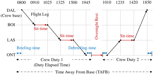
Figure 1: An example of a crew pairing starting from Dallas (DAL) crew base.

The key terms used here, are discussed below. Within a crew pairing, the flight sequence covered in a single working day (not necessarily same as the calendar day) is called a crew duty. In that, a small rest-period, provided between any two flights to facilitate aircraft changes by crew members, is called a sit-time or a connection-time. In contrast, overnight-rest refers to a long rest-period after termination of the current duty and before commencement of the next crew duty. Two short-periods, provided in the beginning and ending of a crew duty, are called briefing and de-briefing time, respectively. The total time elapsed in a duty, including briefing and de-briefing times is called duty elapsed time. Finally, the time elapsed since the start of a crew pairing is called the time away from base (TAFB). At times, a crew is required to be transported to an airport to fly their next flight. In such situations, the crew is transported as passengers in another flight, flown by another crew. Such a flight is called a deadhead or a deadhead flight for the transported crew. The presence of deadhead flights affects an airline’s profit in two ways. Firstly, the airline has to bear the loss of revenue on the passenger seats being occupied by the deadhead-ing crew. Secondly, the airline has to pay the hourly wages to the deadhead-ing crew even when they are not servicing the flight. In order to maximize the profits, airlines desire to minimize these deadheads as much as possible (ideally zero).

2.1 Crew Pairing: Legality Constraints and Costing Criteria

Multiple airline federations (Federal Aviation Administration, European Aviation Safety Agency, etc.) govern the safety of crew members, and, in turn, regulate the ‘legality’ of a crew pairing. Along with this, several other legality constraints linked to airline-specific regulations, labor laws, etc. are required to be satisfied, for a crew pairing to be considered as legal. Broadly, these constraints could be classified as follows:

• Connection-city constraint: this requires the arrival airport of a flight to be the same as the departure airport of the next flight in the pairing sequence.

• Start- & end-city constraint: this requires the departure airport of the first flight and the arrival airport of the last flight, to be the same crew base.

• Sit-time & overnight-rest constraint: this requires the duration of the sit-times and overnight-rests to lie within the lower and upper bounds on the same, as set by airlines in accordance with the federations’ regulation.

• Duty constraints: these cater to the regulations on crew duty, including maximum limits on the permissible - number of duties in a pairing; number of flights in a crew duty; duty elapsed-time and its flying-time, etc.

• Special constraint: Airlines desire to optimize their crew utilization, and formulate some special constraints, such as restricting a pairing which provides for overnights at the same city airports (airports which are in the same city as the crew base), etc.

Given the multiplicity of these constraints, it is important to enable legal crew pairing generation in a time-efficient manner, so that legal crew pairings are available as promptly as possible, when required during the optimization.

The cost of a crew pairing, in general, could be categorized into a flying cost and a non-flying cost (also called variable cost). The former is the cost incurred in actually flying all given flights from an airline’s schedule, and is calculated on an hourly basis. The latter is the cost incurred during the non-flying hours of a pairing, and could further be split into the following costs: (a) Hard cost which includes the hotel cost, meal cost, and the excess pay – the cost associated with the difference between the guaranteed hours of pay and the actual flying hours, and (b) Soft cost which refers to the undesirable cost with associated aircraft changes (during flight-connections), etc.

2.2 CPOP Formulation

It has been mentioned earlier, that CPOP is modeled either as a set partitioning problem or as a set covering problem. The latter allows for more flexibility during its solutioning than the former, by accommodating deadhead flights. In that, for a given set of flights $\mathcal{F}$ (comprising of $F$ flights) that could be covered in multiple ways by a set of legal pairings $\mathcal{P}$ (comprising of $P$ pairings), the aim is to identify that subset of $\mathcal{P}$, say $\mathcal{P}_{IP}^{*}$, which not just covers each flight at least once, but does it at a cost lower than any alternative subset of the $\mathcal{P}$. The task of determining $\mathcal{P}_{IP}^{*}\subseteq\mathcal{P}$ is equivalent to each pairing $p_{j}\in\mathcal{P}$ being either included in $\mathcal{P}_{IP}^{*}$ (marked by the corresponding variable $x_{j}=1$) or excluded from it (marked by the corresponding variable $x_{j}=0$). Notably, each $p_{j}$ is an $F$-dimensional vector, any element of which, say $a_{ij}$, is either $0$ or $1$. In that, if an $i^{th}$ flight ($f_{i}$) is covered by $p_{j}$, then $a_{ij}=1$, else $a_{ij}=0$. In this background, the CPOP formulation (intrinsically an IPP), as employed in this paper, is presented below.

$$\text{Min.}~{}Z_{IP}=\sum_{j=1}^{P}c_{j}x_{j}+\psi_{D}\cdot\left(\sum_{i=1}^{F}\left(\sum_{j=1}^{P}a_{ij}x_{j}-1\right)\right),$$ (1)

$$\text{subject to}\quad\sum_{j=1}^{P}a_{ij}x_{j}\geq 1,\quad~{}~{}~{}~{}~{}\forall i\in\{1,2,...,F\}$$ (2)

$$\qquad\qquad\quad x_{j}\in\mathbb{Z}=\{0,1\},~{}~{}~{}~{}\forall j\in\{1,2,...,P\}$$ (3)

$$\text{where},c_{j} :~{}\text{the cost of a legal pairing }p_{j},$$

$$\psi_{D} :~{}\text{an airline-defined penalty cost against each deadhead in the solution},$$

$$\quad a_{ij} =~{}1,~{}\text{if flight}~{}f_{i}~{}\text{is covered in pairing}~{}p_{j};~{}else~{}0$$

$$x_{j} =~{}1,~{}\text{if pairing}~{}p_{j}~{}\text{contributes to Minimum}~{}Z;~{}else~{}0$$

In Equation 1, the first cost component represents the sum of the individual cost of the pairings, while the second component represents the penalty cost for the deadheads in the solution (note, $(\sum_{j=1}^{P}a_{ij}x_{j}-1)$ represents the number of deadheads corresponding to an $i^{th}$ flight in the solution). Notably, the above formulation assumes that the set of all possible pairings, namely, $\mathcal{P}$, are available apriori, and the task is to determine the set $\mathcal{P}_{IP}^{*}$. However, due to the practical challenge associated with generation of $\mathcal{P}$ apriori (as cited in Section 1), solution to the IPP is pursued in conjunction with the corresponding LPP (formulation deferred till Section 4) assisted by CG technique.

3 Overview of AirCROP - the testbed for the Proposed CG heuristic

As a prelude to the proposed CG heuristic (the core of this paper), an overview of AirCROP is presented here, since it serves as a testbed for performance investigation of the heuristic. Its schematic in Figure 2, highlights that it is developed by knitting the following modules – Legal Crew Pairing Generation, Initial Feasible Solution Generation, and CG-driven LPP-solutioning, interactively engaging with IPP-solutioning. The novelty in AirCROP lies in not just how each module (briefed below) is conceived and implemented, but also in how these modules interact. An overview of these modules is presented in the following sub-sections. However, for a comprehensive discussion on their interactions, interested readers are referred to Aggarwal et al. (Unpublished results, 2020a).

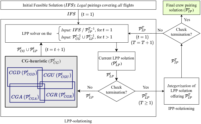
Figure 2: A schematic for AirCROP, enabled by the proposed CG heuristic, comprising of the following strategies to generate fresh pairings $\mathcal{P}_{CG}^{t}$ at any LPP iteration $t$: Deadhead reduction ($CGD$, generating $\mathcal{P}_{CGD}^{t}$), Crew Utilization enhancement ($CGU$, generating $\mathcal{P}_{CGU}^{t}$), Archiving ($CGA$, generating $\mathcal{P}_{CGA}^{t}$), and Random exploration ($CGR$, generating $\mathcal{P}_{CGR}^{t}$). $T$ marks the counter to track the interactions between IPP- and LPP-solutioning.

3.1 Legal Crew Pairing Generation

This module helps generate pairings which satisfy all the legality constraints. Such legal pairings enable generation of an initial feasible solution, and also feed real-time in to the proposed CG heuristic towards LPP-solutioning. Alarmingly, Klabjan and Schwan (2001) have inferred based on empirical evidence, that typically 80% of the CPOP-solutioning time may be consumed by legal pairings’ generation. Considering that this challenge may only be augmented for complex flight networks, the following preemptive measures have been implemented, given which the total time spent on legal crew pairing generation ranges from $25$ to $50\%$ of the overall run-time for AirCROP, depending on the scale and complexity of the underlying data set (Aggarwal et al., 2018):

• adoption of duty-network: here, all possible legal crew duties are generated apriori by accounting for several duty constitutive constraints, including connection-city and sit-time constraints. Such duties are then used to generate pairings, avoiding the need to re-evaluate several constraints, when pairings are needed in real-time.

• overnight-rest constraints’ preprocessing: here, a duty overnight-connection graph is pre-processed by satisfying the overnight-rest constraint between all possible pairs of apriori generated legal duties, eliminating the need for its repeated evaluation, when pairings are needed.

• crew base driven parallelization: recognizing, that duty constraints do vary across the different crew bases, legal pairing generation process is decomposed into independent sub-processes, capable of running in parallel on multiple cores of a single processing unit.

3.2 Initial Feasible Solution Generation

This module aims to generate an initial feasible solution (IFS) – a manageable set of legal crew pairings covering all flights in a given schedule. For large-scale CPOPs, IFS generation standalone is computationally challenging as it constitutes an NP-complete problem. For AirCROP, a time-efficient IFS-generation heuristic, namely, an Integer Programming based Divide-and-cover Heuristic has been implemented (Aggarwal et al., Unpublished results, 2020b). It relies on: (i) a divide-and-cover strategy to decompose the input flight schedule into smaller flight subsets, and (ii) use of integer programming to find quality set of pairings for each decomposed flight subset.

3.3 Interactive CG-driven LPP- and IPP-solutioning

This is the core optimization module, which relies on intermittent interaction of submodules, as briefed below:

• LPP-solutioning: as highlighted in Figure 2, this phase entails several iterations ($t$) of an LPP solver until the termination criterion is not met. In that, if the cost improvements over a pre-specified number of successive LPP iterations falls below a pre-specified threshold (highlighted in Section 5.2), this phase is terminated. In the initial iteration ($t=1$), the input set is nothing but the IFS. In any subsequent iteration $t$, the input set comprises of the previous iteration’s– LPP solution $\mathcal{P}_{LP}^{t-1}$ and a fresh set of pairings generated/re-inducted using the proposed CG heuristic ($\mathcal{P}_{CG}^{t-1}$). This input pairing set is fed into the LPP solver to find the current $\mathcal{P}_{LP}^{t}$, which is further used by the proposed CG heuristic to generate a fresh set of pairings $\mathcal{P}_{CG}^{t}$. While the details of the proposed CG heuristic are presented in the next section, it may be noted here, that the composition of $\mathcal{P}_{CG}^{t}$ is guided by a two-pronged strategy of exploring the new pairings’ space on the one hand, and utilizing the efficient pairings encountered over the past LPP iterations on the other. In that:

  • exploring the new pairings’ space: this is guided by three strategies, namely, deadhead reduction ($CGD$), crew utilization enhancement ($CGU$), and random exploration of pairings’ space ($CGR$). Notably, the former two strategies pursue the desired optimal solution features.

  • utilizing the efficient pairings from the past: this is guided by the archiving strategy ($CGA$) which utilizes the dual variables of the current LPP solution to identify the promising flight-pairs, corresponding to which efficient pairings from the archive of the past LPP iterations, are extracted.

• IPP-solutioning: once a particular phase of LPP-solutioning terminates, the LPP solution is passed over for its integerization, towards which the branch-and-bound algorithm is used. Being a minimization problem, this algorithm maintains the valid lower bound (LPP solution) and the best upper bound (IPP solution) at each node of its search-tree, and it terminates itself if the difference between these two bounds (MIP gap) becomes zero. However, the branch-and-bound search on a large-scale IPP is time-intensive. Hence, the algorithm is terminated at a pre-defined time limit (highlighted in Section 5.2), if it does not self-terminate apriori. Subsequently, the corresponding IPP solution is passed back as the input for the next phase of LPP-solutioning.

Notably, the LPP- and IPP-solutioning interactions are tracked through the $T$ count, and in principle AirCROP is terminated when the cost of the IPP solution ($Z_{IP}^{T}$ corresponding to $\mathcal{P}_{IP}^{T}$) matches the cost of its input LPP solution ($Z_{LP}^{T}$ corresponding to $\mathcal{P}_{LP}^{T}$). However, for practical considerations on the time limit, if the IPP and LPP costs do not conform with each other despite a pre-specified number of LPP-IPP interactions, or up to a pre-specified limit on the total run-time, the termination of AirCROP is enforced (these pre-specified numbers are highlighted in Section 5.2). It may also be noted that aligned with the scope of this paper, all features and associated parameters in AirCROP but for the combinations of CG strategies, are uniformly maintained for experimentation and results.

4 Domain-knowledge Inspired Column Generation Heuristic

The aim in this paper is to demonstrate the efficacy of the proposed CG heuristic towards fulfilling the overarching aim of solving the CPOP/IPP problem (Equations 1 to 3) within the AirCROP architecture (Figure 2). Notably, the prerequisite for solving the IPP formulation is that the set of all possible legal pairings $\mathcal{P}$ is generated apriori. Considering, this may be computationally-intractable for large-scale/complex flight networks, AirCROP relies on first solving the corresponding LPP (formulated below), and integerization of the resulting LPP solution, over multiple such interactions. Solution to LPP is obtained by iteratively invoking an LPP solver. In the first iteration, the input to an LPP solver is any set of pairings covering all the scheduled flights. In any subsequent iteration, the new input set comprises of the previous iteration’s– LPP solution and a set of fresh pairings promising further improvement in the objective function, as generated/re-inducted using the proposed CG heuristic. In other words, the quality of the final LPP solution is directly dependent on the efficacy of the CG heuristic. Furthermore, whenever an LPP solution is passed on for its integerization (IPP-solutioning), the objective function value for the LPP solution marks the lower bound for the corresponding Integer solution. In other words, an integer solution can not have a better objective function value than the underlying LPP solution. It implies that after several interactions of LPP- and IPP-solutioning, the quality of the final IPP solution would also depend on the search efficiency in the LPP solutioning phase, at the core of which lies the CG heuristic. This is a testament to the importance of the proposed CG heuristic and this paper.

The details and associated nitty-gritty of the proposed CG heuristic can be best explained at the level of each LPP iteration ($t$), that could be perceived as being implemented in three phases. In that:

• firstly, for a given set of input pairings, LPP solver is invoked on the primal form of the LPP formulation (Equations 4 to 6), and the LPP solution is obtained, in that, each pairing $p_{j}$ in the input set gets assigned a value $x_{j}$ varying from $0$ to $1$. All the $x_{j}$s together constitute the primal variable vector, notated as $X=[x_{1}~{}x_{2}~{}x_{3}~{}...~{}x_{P}]^{\mathsf{T}}$. Furthermore, the elements in $X$ with non-zero values ($x_{j}\neq 0$), and the set of underlying pairings are notated as $X_{LP}$ and $\mathcal{P}_{LP}$, respectively.

  $$\text{Min.}~{}Z_{LP}^{p}=\sum_{j=1}^{P}c_{j}x_{j}+\psi_{D}\cdot\left(\sum_{i=1}^{F}\left(\sum_{j=1}^{P}a_{ij}x_{j}-1\right)\right)=\sum_{j=1}^{P}\left(c_{j}+\psi_{D}\cdot\sum_{i=1}^{F}a_{ij}\right)x_{j}-F\cdot\psi_{D},$$ (4)

  $$\text{subject to}\quad\sum_{j=1}^{P}a_{ij}x_{j}\geq 1,\qquad\quad\forall i\in\{1,2,...,F\}$$ (5)

  $$\qquad\qquad\quad x_{j}\in\mathbb{R}=[0,1],\qquad\forall j\in\{1,2,...,P\}$$ (6)

  Notably, the contribution of each pairing to the LPP solution (Equation 6), could be effectively treated as:

  $$\qquad\qquad\quad x_{j}\in\mathbb{R}\geq 0,\qquad\quad~{}~{}\forall j\in\{1,2,...,P\}$$ (7)

  The rationale is that minimization of $Z_{LP}^{p}$ will always lead to a solution with all variables $x_{j}\leq 1$ (Vazirani, 2003). Hence, the primal form of the LPP is represented by Equations 4, 5 & 7. Here, the use of Equation 7 instead of Equation 6, helps in getting rid of an additional dual variable in the dual form of the LPP formulation, as defined in the subsequent text.

• secondly, the pairing set $\mathcal{P}_{LP}$ is fed to the dual form of the LPP formulation (Equations 8 to 10), and LPP solver is invoked to yield the dual variable vector $Y=[y_{1}~{}y_{2}~{}y_{3}~{}...~{}y_{F}]^{\mathsf{T}}$ corresponding to the flight constraints.

  $$\text{Max.}~{}Z_{LP}^{d}=\sum_{i=1}^{F}y_{i}-F\cdot\psi_{D},$$ (8)

  $$\text{subject to}\quad\sum_{i=1}^{F}a_{ij}y_{i}\leq\left(c_{j}+\psi_{D}\cdot\sum_{i=1}^{F}a_{ij}\right),~{}~{}~{}~{}\forall j\in\{1,2,...,P_{LP}\}$$ (9)

  $$\qquad\qquad\qquad\quad~{}~{}y_{i}\in\mathbb{R}\geq 0,\qquad\qquad\qquad~{}~{}~{}~{}\forall i\in\{1,2,...,F\}$$ (10)

  $$\text{where},\quad P_{LP}:~{}\text{is the number of pairings in the set}~{}\mathcal{P}_{LP}$$

  $$\qquad\qquad y_{i}:~{}\text{dual variable, corresponding to an $i^{th}$ flight-coverage constraint},$$

• availability of the dual variables paves way for the pricing sub-problem, where the aim is to generate those legal pairings which if included as part of the input to the next LPP iteration, promise a better $Z_{LP}^{p}$ than the current. The standard CG technique (with exact-pricing strategy, as mentioned in Section 1.1) identifies only the pairings with most negative reduced cost values, where, the reduced cost ($\mu_{j}$) is, as defined in Equation 11.

  $$\mu_{j}=\left(c_{j}+\psi_{D}\cdot\sum_{i=1}^{F}a_{ij}\right)-\mu d_{j},~{}\text{where,}~{}\mu d_{j}=\sum_{i=1}^{F}a_{ij}\cdot y_{i}~{}~{}(~{}\text{represents dual cost component of}~{}\mu_{j})$$ (11)

  Here, the potential of a pairing to further reduce $Z_{LP}^{p}$ is in proportion to the magnitude of its $\mu_{j}$ value. Notably, the distinctive contribution of the proposed CG heuristic lies in the fact, that from within the larger pool of pairings with negative $\mu_{j}$, besides selecting pairings randomly, it also selects pairings in a guided manner. In that, selection of such pairings is guided by optimal solution features at a set level and individual pairing level, and utilization of the past computational effort. Once a set of such promising pairings meets a pre-defined size, it is merged with the existing $\mathcal{P}_{LP}$, and fed as the input for the next LPP iteration. When repeated, this procedure leads to a near-optimal LPP solution which could be integerized.

In essence, while the standard CG technique prioritizes the generation of only the pairings with most negative $\mu_{j}$ to qualify as an input for the next LPP iteration, the proposed CG heuristic prioritizes the generation of some pairings over the others amongst the pool of pairings with negative $\mu_{j}$, through its multi-pronged strategies, including:

• Deadhead reduction strategy, $CGD$: prioritizes a set of legal pairings that is characterized by low deadheads - a feature which domain knowledge recommends for optimality at a set level.

• Crew Utilization enhancement strategy, $CGU$: prioritizes a set of legal pairings, each member of which is characterized by high crew utilization - a feature which domain knowledge recommends for optimality at a pairing level.

• Archiving strategy, $CGA$: prioritizes a set of legal pairings comprising of those flight-pairs, which as per the existing LPP solution, bear better potential for improvement in the objective function. Such a set, originating from the flight-pair level information, is extracted from an archive of previously generated pairings. In doing so, this strategy facilitates utilization of the past computational efforts, by providing an opportunity for an earlier generated legal pairing to be re-inducted in the current pairing pool.

• Random exploration strategy, $CGR$: unlike $CGU$ and $CGD$ which are guided by the desired optimal solution features, and $CGA$ which is guided by the existing LPP solution features, this strategy pursues random and unbiased exploration of pairings’ space.

In this background, the details of each strategy leading upto the proposed CG heuristic are presented below.

4.1 Deadhead Reduction Strategy ($CGD$)

As mentioned earlier, a deadhead flight adversely affects an airline’s profit. Hence, airlines desire to minimize the deadhead flights as much as possible (ideally zero). Towards it, while defining the costing criteria for a pairing, airlines include a high penalty cost for each deadhead flight present in a crew pairing solution. It implies that while pursuing minimization of the total cost, the resulting solution shall also be characterized by minimal possible deadheads. To exploit this optimality feature, the deadhead reduction strategy ($CGD$) proposed here, aims to generate a new pairing set, $\mathcal{P}^{t}_{CGD}$, which provides an alternative way to cover the flights involved in a subset of $\mathcal{P}^{t}_{LP}$, while also ensuring that some of these flights get covered with zero deadheads. This strategy promises propogation of the zero-deadhead feature over successive LPP iterations for the following reasons:

• $\mathcal{P}^{t}_{CGD}$ alongside $\mathcal{P}^{t}_{LP}$ forms a part of the input for the next LPP iteration

• $\mathcal{P}^{t}_{CGD}$ provides a scope for better coverage (zero-deadhead) of some flights, compared to $\mathcal{P}^{t}_{LP}$

• $\mathcal{P}^{t}_{CGD}$ may focus on zero-deadhead coverage for different flights in different LPP iterations

The implementation of this strategy at iteration $t$, formalized in Algorithm 1, has been explained below in conjunction with Figure 3 (where, a sample $\mathcal{P}^{t}_{LP}$ comprises of pairings $p_{1}$ to $p_{9}$, to cover the scheduled flights $f_{1}$ to $f_{30}$).

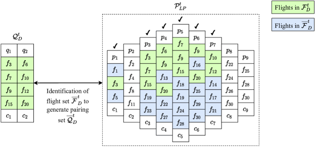
Figure 3: A symbolic depiction of how the deadhead reduction strategy provides for an alternative way to cover the flights involved in a subset of $\mathcal{P}^{t}_{LP}$, while also ensuring that some of these flights get covered with zero deadheads

.

Input: $\mathcal{D}_{all},~{}\mathcal{P}^{t}_{LP},~{}Y^{t},~{}Th_{D}$

Output: $\mathcal{P}^{t}_{CGD}$

1 $Random\leftarrow$ Generate a random integer between 0 & $Th_{D}$

2 $\mathcal{D}_{D}^{t}\leftarrow$ Select $Random$ number of duties, with-respect-to each crew base, from $\mathcal{D}_{all}$ without replacement

Generate all possible pairings using $\mathcal{D}_{D}^{t}$ and compute their $\mu^{t}_{j}$

  $\triangleright$ Use Equation 11

3 Select only the pairings with negative $\mu^{t}_{j}$

4 Sort pairings in ascending order with-respect-to their $\mu^{t}_{j}$

5 $\mathcal{Q}_{D}^{t}\leftarrow$ Select a zero-deadhead pairing set from the sorted pairings

6 $\mathcal{F}_{D}^{t}\leftarrow$ Identify flights covered by pairings in $\mathcal{Q}_{D}^{t}$

7 for each pairing $p_{j}\in\mathcal{P}^{t}_{LP}$ do

8       if pairing $p_{j}$ covers one or more flights from $\mathcal{F}_{D}^{t}$ then

9             $\hskip 1.5pt\vbox{\hrule height=0.5pt\kern 1.35626pt\hbox{\kern-0.90005pt$\mathcal{F}$\kern-0.90005pt}}_{D}^{~{}t}\leftarrow$ Add only those flights from $p_{i}$ that are not present in $\mathcal{F}_{D}^{t}$

10            

11       end if

12      

13 end for

Generate all possible pairings using $\hskip 1.5pt\vbox{\hrule height=0.5pt\kern 1.35626pt\hbox{\kern-0.90005pt$\mathcal{F}$\kern-0.90005pt}}_{D}^{~{}t}$ and compute their $\mu^{t}_{j}$

  $\triangleright$ Use Equation 11

14 $\hskip 1.5pt\vbox{\hrule height=0.5pt\kern 1.35626pt\hbox{\kern-0.90005pt$\mathcal{Q}$\kern-0.90005pt}}_{D}^{~{}t}\leftarrow$ Select only the pairings with negative $\mu^{t}_{j}$

15 $\mathcal{P}^{t}_{CGD}\leftarrow\mathcal{Q}_{D}^{t}\cup\hskip 1.5pt\vbox{\hrule height=0.5pt\kern 1.35626pt\hbox{\kern-0.90005pt$\mathcal{Q}$\kern-0.90005pt}}_{D}^{~{}t}$

16 return $\mathcal{P}^{t}_{CGD}$

Algorithm 1 Procedure for the $CGD$ strategy, at an LPP iteration $t$

The initial step of $CGD$ involves random selection of a subset of legal duties, say $\mathcal{D}^{t}_{D}$, from the set of all legal duties, say $\mathcal{D}_{all}$ (line 2). The maximum number of duties contributing to $\mathcal{D}^{t}_{D}$ with-respect-to each crew base, are limited by a pre-defined threshold, say $Th_{D}$ (the criterion for its setting is highlighted in Section 5.3). The actual number of duties contributing to $\mathcal{D}^{t}_{D}$ with-respect-to each crew base, are guided by $Random$ – a random integer between 0 & $Th_{D}$ (line 1). Subsequently, all possible pairings corresponding to $\mathcal{D}^{t}_{D}$ are generated, of which only those with negative reduced cost ($\mu_{j}^{t}$) are selected (lines 3 & 4). These pairings are then sorted in ascending order with respect to their $\mu_{j}^{t}$ values (line 5), and the largest sized subset characterized by zero deadheads, say $\mathcal{Q}_{D}^{t}$, is extracted using a deterministic approach (line 6). In that, starting with the pairing having the most-negative $\mu_{j}^{t}$ (maximum potential for improvement in the objective), iterations are performed over the sorted pairings, and only those pairings are selected which do not cover an already covered flight. The above sorting is important, since the composition of the zero-deadhead subset is dependent on the order in which pairings are evaluated. Let the set of flights covered by pairings in $\mathcal{Q}_{D}^{t}$ be denoted by $\mathcal{F}_{D}^{t}$ (line 7). Subsequently, $\mathcal{P}_{LP}^{t}$ is scrolled through (lines 8 to 12), and only the pairings covering one or more flights in $\mathcal{F}^{t}_{D}$ are flagged. This enables the composition of $\hskip 1.5pt\vbox{\hrule height=0.5pt\kern 1.50696pt\hbox{\kern-1.00006pt$\mathcal{F}$\kern-1.00006pt}}^{~{}t}_{D}$ (line 10) as the set of complementary flights – those which are not present in $\mathcal{F}^{t}_{D}$. For instance, in Figure 3, $\mathcal{Q}^{t}_{D}=\{q_{1},q_{2}\}$, $\mathcal{F}^{t}_{D}=\{f_{3},~{}f_{6},~{}f_{7},~{}f_{9},~{}f_{10},~{}f_{12},~{}f_{15},~{}f_{20}\}$ (flights in the green colour); pairings $p_{1},~{}p_{3}~{}\ldots~{}p_{7}$ are flagged; and $\hskip 1.5pt\vbox{\hrule height=0.5pt\kern 1.50696pt\hbox{\kern-1.00006pt$\mathcal{F}$\kern-1.00006pt}}^{~{}t}_{D}=\{f_{1},~{}f_{5},~{}f_{13},~{}f_{14},~{}f_{16}~{}\ldots~{}f_{19},~{}f_{21}~{}\ldots~{}f_{25},~{}f_{27}~{}\ldots~{}f_{30}\}$ (flights in the blue colour). Subsequently, all possible pairings corresponding to $\hskip 1.5pt\vbox{\hrule height=0.5pt\kern 1.50696pt\hbox{\kern-1.00006pt$\mathcal{F}$\kern-1.00006pt}}^{~{}t}_{D}$ are generated, of which only those having negative $\mu_{j}^{t}$ values, constitute the set $\hskip 1.5pt\vbox{\hrule height=0.5pt\kern 1.50696pt\hbox{\kern-1.00006pt$\mathcal{Q}$\kern-1.00006pt}}^{~{}t}_{D}$ (lines 13 & 14). Finally, the pairing sets $\mathcal{Q}^{t}_{D}~{}\&~{}\hskip 1.5pt\vbox{\hrule height=0.5pt\kern 1.50696pt\hbox{\kern-1.00006pt$\mathcal{Q}$\kern-1.00006pt}}^{~{}t}_{D}$ jointly constitute $\mathcal{P}^{t}_{CGD}$ (line 15).

4.2 Crew Utilization Enhancement Strategy ($CGU$)

The degree of crew utilization in a pairing can be assessed by the number of hours a crew is at work, out of the maximum permissible working hours, in each of its constituent crew duties. Notably, higher the crew working hours in each duty of a pairing, lower will be its excess pay (Section 2.1). Hence, minimization of the total crew cost is directly linked to the presence of pairings with high crew utilization in the final LPP solution. To exploit this optimality feature, the crew utilization enhancement strategy ($CGU$) proposed here:

• first introduces a new measure, namely, crew utilization ratio ($\gamma_{j}$, Equation 12) to quantify the degree of crew utilization in a pairing $p_{j}$ at any instant

  $$\gamma_{j}=\frac{1}{\text{Number of duties in }p_{j}}\cdot\sum_{d\in p_{j}}\frac{\text{Working hours in duty}~{}d}{\text{Permissible hours of duty }d}$$ (12)

• identifies with reference to $\mathcal{P}^{t}_{LP}$, pairings characterized by high dual cost component ($\mu d_{j}^{t}$, Equation 11), reflecting in turn on the constitutive flights with high value of dual variables ($y_{i}^{t}$, Equation 11)), and hence, on the potential of these flights to generate new pairings with more negative $\mu_{j}^{t}$

• utilizes the flight information to generate promising pairings, and picks the ones with high $\gamma_{j}^{t}$ to constitute $\mathcal{P}^{t}_{CGU}$.

This strategy promises propogation of the higher crew utilization ratio over successive LPP iterations, given that in each LPP iteration $\mathcal{P}^{t}_{CGU}$ alongside $\mathcal{P}^{t}_{LP}$ forms a part of the input for the next iteration.

The implementation of this strategy at iteration $t$, formalized in Algorithm 2, has been explained below in conjunction with Figure 4 (where, a sample $\mathcal{P}^{t}_{LP}$ comprises of pairings $p_{1}$ to $p_{4}$, covering the flights $f_{1}$ to $f_{13}$).

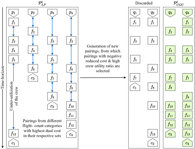
Figure 4: A symbolic depiction of how the crew utilization enhancement strategy provides for novel flight-connections, enabling generation of new pairings with high crew utilization ratio

Input: $\mathcal{P}^{t}_{LP},~{}X_{LP}^{t},~{}Y^{t},~{}Th_{U}$

Output: $\mathcal{P}^{t}_{CGU}$

1 $Dictionary\leftarrow$ Categorize pairings in $\mathcal{P}^{t}_{LP}$ with-respect-to flight-counts $Random\leftarrow$ Generate a random integer between 0 & $Th_{U}$ while $|\mathcal{F}_{U}^{t}|<Random$ do

       Select a random $(k,\mathcal{P}_{k}^{t})$ pair from $Dictionary$ without replacementCompute $\mu d_{j}^{t}$ values for pairings in $\mathcal{P}^{t}_{k}$  $\triangleright$ Use Equation 11

2       Sort pairings in $\mathcal{P}^{t}_{k}$ in descending order with-respect-to their $\mu d^{t}_{j}$ & $x_{j}~{}(\in X_{LP}^{t})$ $Counter\leftarrow 0$ for each pairing $p_{j}\in\mathcal{P}^{t}_{k}$ do

3             $\mathcal{F}_{U}^{t}\leftarrow$ Add flights covered in $p_{j}$ $Counter\mathrel{+}=$ Number of flights in $p_{j}$ if $Counter\geq Random/(k_{max}-k_{min})$ then

4                   Break

5             end if

6            

7       end for

8      

9 end while

Generate all possible pairings using $\mathcal{F}_{U}^{t}$ and select only the pairings with negative $\mu^{t}_{j}$ Compute $\gamma_{j}^{t}$ of the selected pairings and find the median value   $\triangleright$ Use Equation 12

$\mathcal{P}^{t}_{CGU}\leftarrow$ Select only the pairings with $\gamma_{j}^{t}\geq$ the median value return $\mathcal{P}^{t}_{CGU}$

Algorithm 2 Procedure for the $CGU$ strategy, at an LPP iteration $t$

In that:

• firstly, all pairings in $\mathcal{P}^{t}_{LP}$ are categorized with-respect-to the number of flights covered in them (flight-count), denoted by $k$. The range of $k$ is given by the upper and lower bounds, denoted by $k_{max}$ and $k_{min}$, respectively

• secondly, a $Dictionary$ is constituted, each element of which can be given by $(k,\mathcal{P}_{k}^{t})$, where, $\mathcal{P}_{k}^{t}$ represents the set of pairings corresponding to flight count $k$ (line 1). The rationale is to identify promising flights corresponding to each $k$, so that their collective set ($\mathcal{F}_{U}^{t}$, formed over all the $k$s), has a better chance to offer pairings with higher flight-count and crew utilization ratio. The size of $\mathcal{F}_{U}^{t}$ is controlled by $Random$ – a random integer between 0 and a pre-defined upper threshold, namely, $Th_{U}$ (the criterion for its setting is highlighted in Section 5.3).

• subsequently, $\mathcal{F}_{U}^{t}$ is composed iteratively, where each iteration involves:

  • random selection of a $(k,\mathcal{P}_{k}^{t})$ category from the $Dictionary$ without replacement (line 4)

  • computation of each pairing’s $\mu d_{j}^{t}$ (line 5), and subsequently their sorting by descending order of their $\mu d_{j}^{t}$, or by their primal variables $x_{j}^{t}$ in case of a tie in $\mu d_{j}^{t}$ values (line 6)

  • sequential scrolling of the sorted pairings, and assignment of each constitutive flight to $\mathcal{F}_{U}^{t}$, until the flights add up to the limit permissible for each $k$ category (lines 7 to 14).

• when the size of $\mathcal{F}_{U}^{t}$ exceeds its permissible limit, the iterations are terminated (line 15). Then, all possible pairings with the flights in $\mathcal{F}_{U}^{t}$ are generated, and only those with negative $\mu_{j}^{t}$s are picked, for computation of $\gamma_{j}^{t}$s (lines 16 & 17). Finally, the pairings with above-median $\gamma_{j}^{t}$ values constitute the desired new pairing set, namely $\mathcal{P}_{CGU}^{t}$ (line 18).

To correlate the above procedure with Figure 4, let $p_{1}$, $p_{2}$, $p_{3}$ & $p_{4}$ represent the pairings with highest $\mu d_{j}^{t}$, for $k=5,3,4~{}\&~{}6$, respectively. Hence, all the involved flights shall constitute $\mathcal{F}_{U}^{t}$, leading to several pairings, among which $q_{1}$ to $q_{4}$ are those with negative $\mu_{j}^{t}$s. Finally, $q_{3}$ and $q_{4}$ constitute $\mathcal{P}_{CGU}^{t}$, owing to their above-median $\gamma_{j}^{t}$s.

4.3 Archiving Strategy ($CGA$)

It may be noted that in a combinatorial optimization problem like CPOP, if a legal pairing that is part of the input for an LPP iteration, fails to be a part of the LPP solution, then it does not imply that the pairing is of no-use in absolute sense. It only implies that in that particular iteration, it did not fit among the combinations of other pairings leading to an optimal solution. Hence, it is only logical that such a pairing is re-inducted as part of the input for a subsequent iteration too. It is all the more imperative, considering that generation of legal pairing is a computationally demanding and time consuming task. Towards it, an exploratory attempt is made by the authors in Aggarwal et al. (Unpublished results, 2020d). In that, though a considerable amount of cost-improvement is observed in the LPP-solutioning phases of the optimizer, the total run-time of the optimizer increased drastically. This became the motivation for the development of the archiving strategy ($CGA$) proposed here. In any iteration $t$, $CGA$:

• maintains an archive $\mathcal{A}^{t}$ of the previously generated pairings, such that any pairing is stored/retrieved with reference to a unique index $(f_{m},f_{n})$ reserved for any legal flight-pair in that pairing.

• introduces a new measure, namely, reduced cost estimator ($\eta_{mn}^{t}$, Equation 13) for a flight-pair in $\mathcal{A}^{t}$, indexed as $(f_{m},f_{n})$. This estimator can be computed for all the flight-pairs present across all the pairings in the current LPP solution (by fetching $f_{m}$, $f_{n}$, $y_{m}$ and $y_{n}$).

  $$\eta_{mn}^{t} =flying\_cost(f_{m})+flying\_cost(f_{n})-y^{t}_{m}-y^{t}_{n}=\sum_{i\in\{m,n\}}\left(flying\_cost(f_{i})-y^{t}_{i}\right)$$ (13)

  Notably, this formulation is analogous to Equation 11, just that instead of complete cost for a pairing, only the flying costs corresponding to the flights in a legal pair, are accounted for. Given this, $\eta_{mn}^{t}$ may be seen as an indicator of $\mu_{j}$ at the flight-pair level.

• recognizes that towards further improvement in the current LPP solution, it may be prudent to include as a part of the input for next LPP iteration – fresh pairings comprising of flight-pairs with low $\eta_{mn}^{t}$. To this effect, $\mathcal{P}^{t}_{CGA}$ is in principle constituted by preferentially picking pairings in $\mathcal{A}^{t}$ comprising of flight-pairs reporting lower $\eta_{mn}^{t}$.

In doing so, this strategy pursues the goal of continual improvement in the objective function, while relying on the flight-pair level information embedded in the LPP solution at any iteration, and utilizing the past computational efforts.

Input: $\mathcal{A}^{t-1},~{}\mathcal{P}^{t-1}_{LP}\cup\mathcal{P}^{t-1}_{CG},~{}Y^{t},~{}Th_{A}$

Output: $\mathcal{P}^{t}_{CGA}$

$\mathcal{A}^{t}\leftarrow$ Update $\mathcal{A}^{t-1}$ with each pairing $p_{j}\in\mathcal{P}^{t-1}_{LP}\cup\mathcal{P}^{t-1}_{CG}$ $Random\leftarrow$ Generate a random integer between 0 & $Th_{A}$ Compute $\eta^{t}_{mn}$ for each flight-pair $(f_{m},f_{n})\in\mathcal{A}^{t}$  $\triangleright$ Use Equation 13

1 Sort elements of $\mathcal{A}^{t}$ in ascending order with-respect-to the $\eta^{t}_{mn}$s of the corresponding flight-pairs for each element $\left((f_{m},f_{n}),\mathcal{P}_{mn}^{t}\right)\in~{}sorted~{}\mathcal{A}^{t}$ do

2       $\mathcal{P}_{A}^{t}\leftarrow$ Randomly select a maximum of $Random$ number of pairings from $\mathcal{P}_{mn}^{t}$ if $|\mathcal{P}_{A}^{t}|\geq(Random\cdot Random)$ then

3             Break

4       end if

5      

6 end for

Compute $\mu^{t}_{j}$ of all pairings in $\mathcal{P}_{A}^{t}$  $\triangleright$ Use Equation 11

$\mathcal{P}^{t}_{CGA}\leftarrow$ Select only the pairings with negative $\mu_{j}^{t}$ from $\mathcal{P}_{A}^{t}$ return $\mathcal{P}^{t}_{CGA}$

Algorithm 3 Procedure for the $CGA$ strategy, at an LPP iteration $t$

The implementation of this strategy at iteration $t$, has been formalized in Algorithm 3. In that, the first step is to obtain an updated archive, $\mathcal{A}^{t}$ (line 1), by conjoining the previous archive $\mathcal{A}^{t-1}$ and the set of pairings received as input from the previous iteration. Here, $\mathcal{A}^{t}$ is a dictionary, each element of which can be given by $\left((f_{m},f_{n}),\mathcal{P}^{t}_{mn}\right)$, where $(f_{m},f_{n})$ is a legal flight-pair and $\mathcal{P}^{t}_{mn}$ – the corresponding pairing set. In the first iteration ($t=1$), the archive $\mathcal{A}^{1}$ is created using the pairings from the initial feasible solution. Notably, with generation of approximately a million pairings in each LPP iteration, the size of $\mathcal{A}^{t}$ grows at an alarming rate. Hence, for tractability, this strategy extracts only a subset of pairings, say $\mathcal{P}_{A}^{t}$, from the current archive $\mathcal{A}^{t}$. The size of $\mathcal{P}_{A}^{t}$ is controlled at two levels, by $Random$ – a random integer between $0$ and a pre-defined upper threshold, namely, $Th_{A}$ (the criterion for its setting is highlighted in Section 5.3). In that:

• firstly, $\eta_{mn}^{t}$ is computed for each flight-pair in $\mathcal{A}^{t}$ (line 3), allowing for sorting of these pairs in ascending order of their $\eta_{mn}^{t}$ values (line 4). Then the first $Random$ flight-pairs from the sorted list are considered (lines 2 to 5).

• subsequently, for each considered flight-pair, $(f_{m},f_{n})$, a fixed number of pairings are selected randomly from $\mathcal{P}^{t}_{mn}$, and this number is also same as $Random$ (lines 6 to 9).

Once $\mathcal{P}_{A}^{t}$ is constituted as above, $\mu_{j}^{t}$ is computed (line 11) for each of its pairings, and those with negative $\mu_{j}^{t}$ values are selected to constitute the new pairing set, namely $\mathcal{P}_{CGA}^{t}$ (line 12).

4.4 Random Exploration Strategy ($CGR$)

It is critical to note that each of the CG strategy presented above: (a) deadhead reduction ($CGR$ offering $\mathcal{P}_{CGD}^{t}$) pursuing optimal features at a set level, (b) crew utilization enhancement ($CGU$ offering $\mathcal{P}_{CGU}^{t}$) pursuing optimal features at a pairing level, and (c) archiving ($CGA$ offering $\mathcal{P}_{CGA}^{t}$) based on a flight-pair level information, involves the use of current LPP solution. In contrast, the random exploration strategy proposed here, namely, $CGR$ aims to pursue random and unbiased exploration of the pairings’ space, independent of the current LPP solution. It involves generation of new pairings for a random selected set of legal duties, of which only the pairings with negative reduced cost are selected to constitute a new pairing set, $\mathcal{P}_{CGR}^{t}$. Here, a random set of legal duties is used instead of a random set of flights, as the former has a higher probability of generating legal pairings, given that satisfaction of most of the legality constraints is ensured during their pre-processing.

Input: $\mathcal{D}_{all},~{}Y^{t},~{}Th_{R}$

Output: $\mathcal{P}^{t}_{CGR}$

$Random\leftarrow$ Generate a random integer between 0 & $Th_{R}$ $\mathcal{D}_{R}^{t}\leftarrow$ Select $Random$ number of duties with-respect-to each crew base, from $\mathcal{D}_{all}$ without replacement Generate all possible pairings using $\mathcal{D}_{R}^{t}$ and compute their $\mu^{t}_{j}$  $\triangleright$ Use Equation 11

$\mathcal{P}^{t}_{CGR}\leftarrow$ Select only the pairings with negative $\mu^{t}_{j}$ return $\mathcal{P}^{t}_{CGR}$

Algorithm 4 Procedure for the $CGR$ strategy, at an LPP iteration $t$

The implementation of this strategy at iteration $t$, has been formalized in Algorithm 4. Its input involves the set of all legal duties $\mathcal{D}_{all}$, the dual vector $Y^{t}$, and a pre-defined threshold, denoted by $Th_{R}$ (the criterion for its setting is highlighted in Section 5.3). A random integer between $0$ and $Th_{R}$, namely, $Random$, defines the number of duties with-respect-to each crew base, for which new pairings are to be generated. This cumulatively helps constitute the subset of legal duties, $\mathcal{D}^{t}_{R}$ (line 2), for which pairings are generated and the corresponding $\mu_{j}^{t}$ values are computed (line 3). Finally, only the pairings with negative $\mu_{j}^{t}$ values constitute $\mathcal{P}^{t}_{CGR}$ (line 4), which forms a part of the input for the next LPP iteration.

Overarching CG heuristic based on the four CG strategies
In the wake of the context set up early in this section, and the CG strategies, namely, $CGD$, $CGU$, $CGA$ & $CGR$, discussed individually, the overarching CG heuristic has been presented in the Algorithm 5.

Input: $\mathcal{D}_{all},~{}\mathcal{P}^{t}_{LP},~{}X_{LP}^{t},~{}Y^{t},~{}\mathcal{A}^{t-1},~{}\mathcal{P}^{t-1}_{CG}\cup\mathcal{P}^{t-1}_{LP},~{}Th_{R},~{}Th_{U},~{}Th_{D},~{}Th_{A}$

Output: $\mathcal{P}_{CG}^{t}$

$\mathcal{P}^{t}_{CGD}\leftarrow CGD(\mathcal{D}_{all},\mathcal{P}^{t}_{LP},Y^{t},Th_{D})$ $\mathcal{P}^{t}_{CGU}\leftarrow CGU(\mathcal{P}^{t}_{LP},X_{LP}^{t},Y^{t},Th_{U})$ $\mathcal{P}^{t}_{CGA}\leftarrow CGA(\mathcal{A}^{t-1},\mathcal{P}^{t-1}_{CG}\cup\mathcal{P}^{t-1}_{LP},Y^{t},Th_{A})$ $\mathcal{P}^{t}_{CGR}\leftarrow CGR(\mathcal{D}_{all},Y^{t},Th_{R})$ $\mathcal{P}_{CG}^{t}\leftarrow\mathcal{P}^{t}_{CGD}\cup\mathcal{P}^{t}_{CGU}\cup\mathcal{P}^{t}_{CGA}\cup\mathcal{P}^{t}_{CGR}$ return $\mathcal{P}_{CG}^{t}$

Algorithm 5 Procedure for the proposed CG heuristic, at an LPP iteration $t$

Notably, the input to the procedure comprises of the set of all legal duties $\mathcal{D}_{all}$, the current LPP solution $\mathcal{P}^{t}_{LP}$, its corresponding primal vector $X_{LP}^{t}$ & dual vector $Y^{t}$, the previous archive $\mathcal{A}^{t-1}$, the pairing set input from the previous iteration $\mathcal{P}^{t-1}_{LP}\cup\mathcal{P}^{t-1}_{CG}$, and the pre-defined thresholds, namely, $Th_{D}$, $Th_{U}$, $Th_{A}$, & $Th_{R}$, for their corresponding CG strategies. It is also evident (lines 1 to 5) that at any given LPP iteration, these CG strategies are executed in a sequential manner, each leading up to a part of the input for the next LPP iteration ($\mathcal{P}^{t}_{CG}$).

5 Computational Experiments

This section presents the test cases used to investigate the performance of the proposed CG heuristic and its underlying strategies. The computational setup and the parameter settings used for this investigation are also highlighted followed by discussion of the experimental results.

5.1 Test Cases

The real-world airline test cases used for experimentation are cited in Table 2. Each of these test cases involves a weekly flight-schedule, and have been provided by the research consortium’s Industrial Sponsor.

Table 2: Real-world airline test cases used in this research work

Test Cases	$\#$Flights	$\#$Crew Bases	$\#$Legal Duties
TC-1	3202	15	454205
TC-2	3228	15	464092
TC-3	3229	15	506272
TC-4	3265	15	446937
TC-5	4212	15	737184

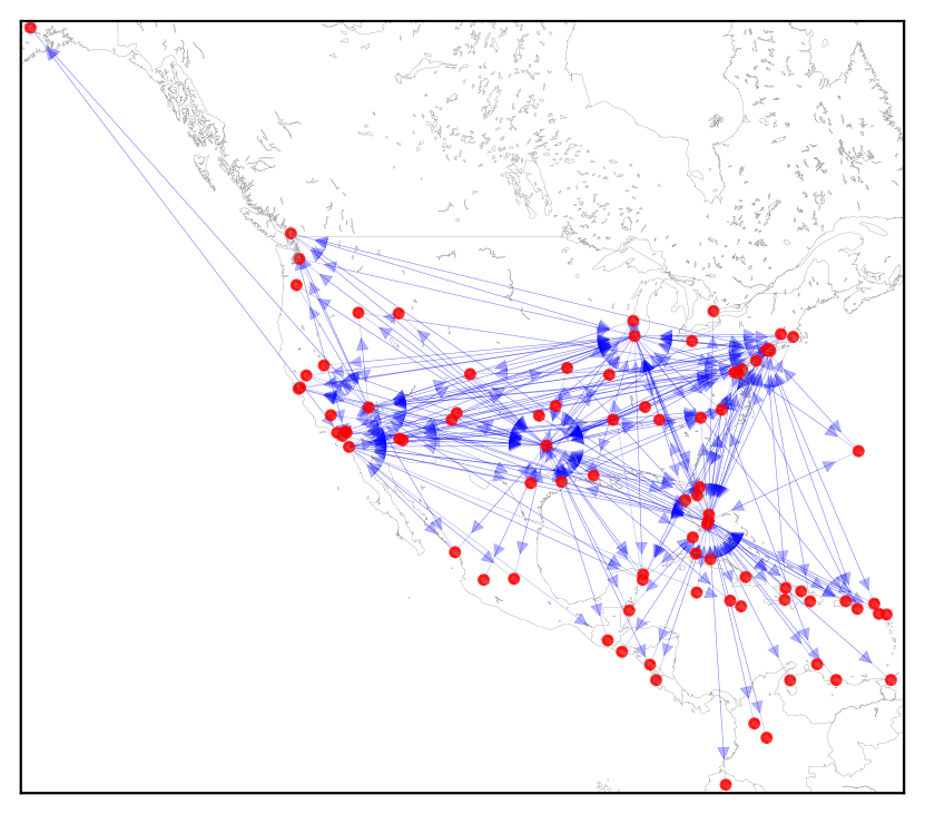
(a)

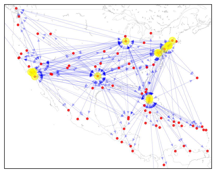
(b)

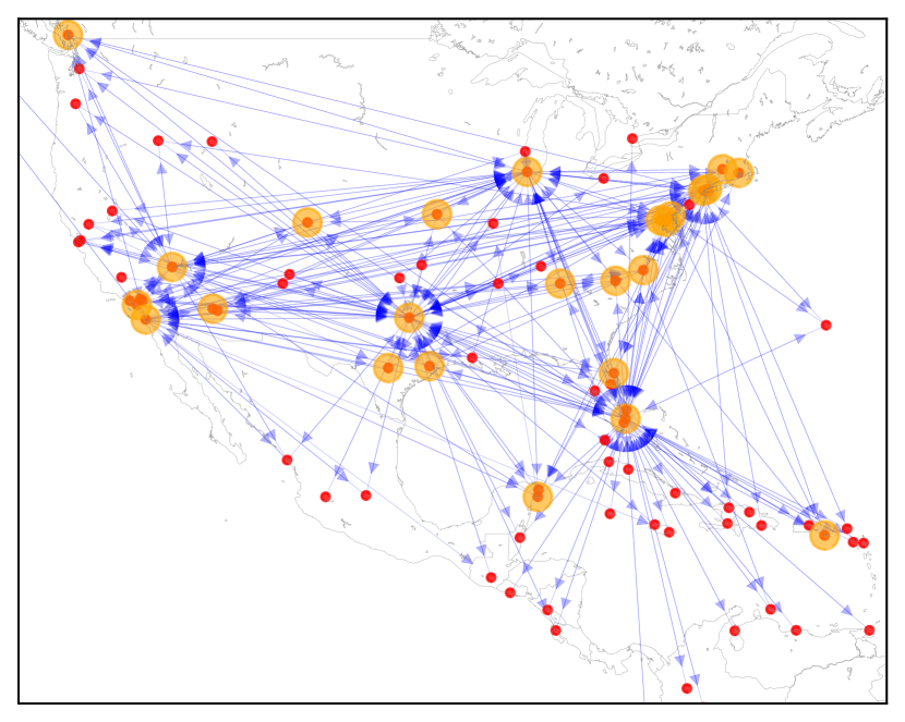
(c)

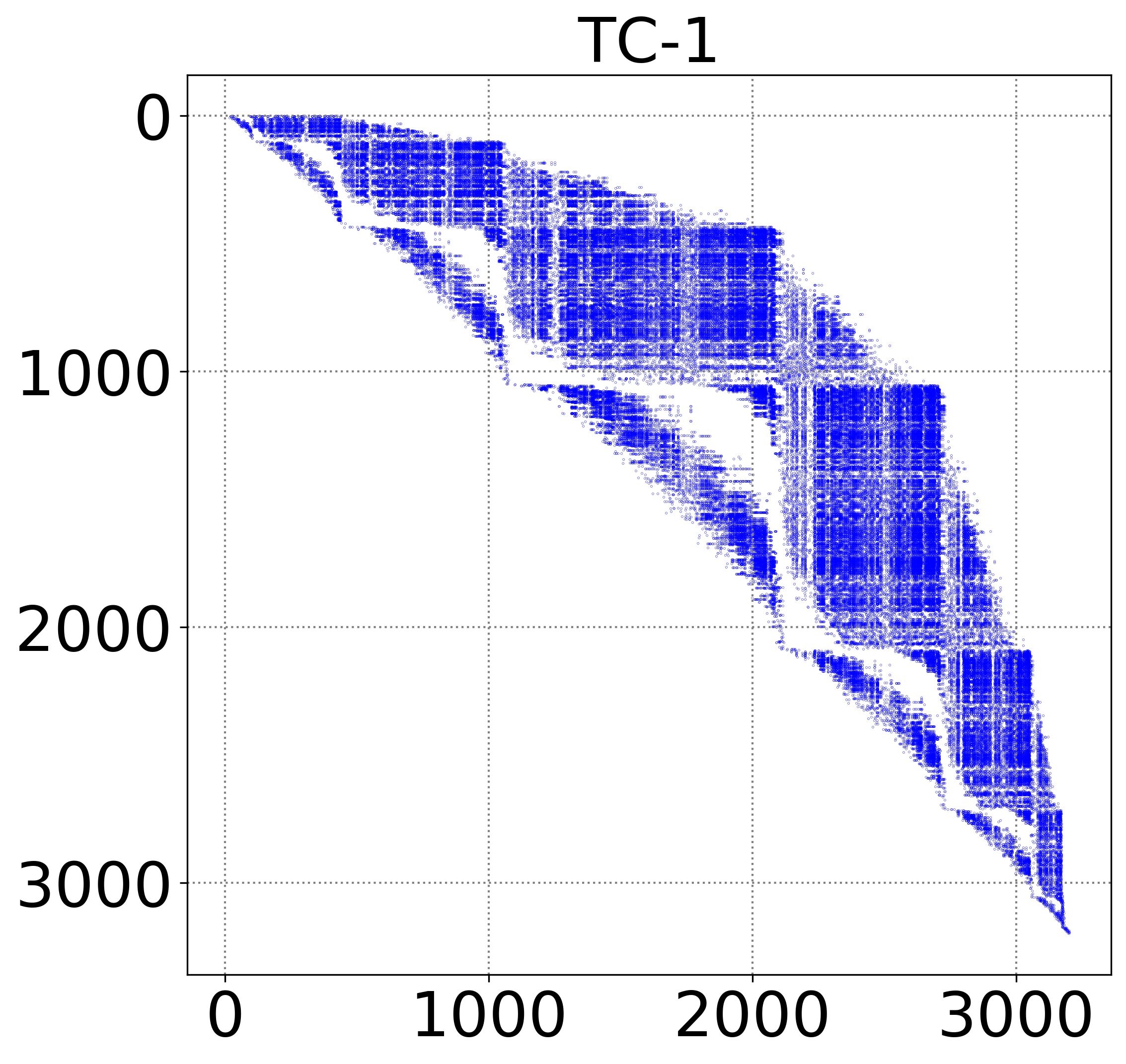
(d)

Figure 5: (a) Geographical representation of TC-1’s flight network, where the red nodes and blue edges represent the airports and scheduled flights, respectively; (b) Zoomed view of TC-1’s flight network with all 15 crew bases highlighted in yellow color; (c) Zoomed view of TC-1’s flight network with major hub airports (serving $\geq$4 other airports) highlighted in orange color; and (d) legal flight-connections, each represented by a point in the plot, where for a flight marked on the y-axis, the connecting flight is marked on the x-axis. Notably, in (d), the flights involved in TC-1 are indexed in the ascending order of their departure time-stamps.

The columns in Table 2, in order of their occurrence, highlight the notations for the different test cases; the number of its constituent flights; the number of constituent crew bases; and the total number of legal duties involved, respectively. It is critical to recognize that the challenge associated with the solutioning of these test cases is attributed to the fact that an inestimably large number of legal pairings are possible for them. This explosion of possible legal pairings is due to not just the large number of flights involved, but also the complexity of the flight networks involved (characterized by multiple crew bases and multiple hub-and-spoke sub-networks), in that, the number of possible legal pairings:

• may grow linearly with the number of crew bases, as they provide the starting and end point for a possible pairing.

• may grow exponentially with the number of hubs involved, as each could serve as an intermediary airport, allowing more flight connections and coverage of more airports within a given duty elapsed time, as opposed to a network with a single hub. This is pertinent particularly when the objective of CPOP encompasses minimization of excess pay which in turn links with maximal utilization of duty elapsed time.

As a sample instance, the geographical representation of the flight network associated with TC-1, its complexity (the presence of multiple crew bases and multiple hub-and-spoke sub-networks) and the legal flight connections involved, are illustrated in Figure 5. In that, the full-scale view of the underlying flight network is portrayed by Figure 5(a). Moreover, Figures 5(b) and 5(c) illustrates a zoomed view of the flight network with all 15 crew bases (highlighted in yellow color) and major hub airports (highlighted in orange color), respectively. Furthermore, the pattern visible in Figure 5(d) could be attributed to the (minimum and maximum) limits on the sit-time and overnight-rest constraints. For instance, a flight, say $f_{500}$, has legal connections only with those flights that depart from the arrival airport of $f_{500}$, and whose departure-time gap (difference between its departure-time and the arrival time of $f_{500}$) lies within the minimum & maximum allowable limit, of the sit-time or the overnight-rest.

5.2 Computational Setup

All the experiments are performed on an HP Z640 Workstation, powered by two Intel^® Xeon^® E5-2630v3 processors, each with 16 cores at 2.40GHz, and 96GB RAM. The codes for AirCROP built around the proposed CG heuristic, are developed using the Python scripting language (aligned with the Industrial sponsor’s larger vision and preference). In that, AirCROP serves as a testbed to investigate the performance of the proposed CG heuristic, and all its features & associated parameters are uniformly maintained for the experimentation. Furthermore:

• In the LPP-solutioning module, the interior-point method from Gurobi Optimizer 8.1.1 (Gurobi Optimization, 2020) is used to solve the primal of the LPP formulation, and the interior-point method (Andersen and Andersen, 2000) from SciPy library (Virtanen et al., 2020) is used to solve the subsequent dual of the LPP formulation. Moreover, the termination of the LPP-solutioning is enforced, if the cost improvement between two successive LPP iterations falls below 100 USD and this trend is successively repeated 10 times. These limits are set to achieve an LPP solution with a sufficiently good cost in a reasonably good time.

• The MIP solver of Gurobi Optimizer 8.1.1 is used in the IPP-solutioning. As mentioned before, the branch-and-bound search on a large-scale IPP is time-intensive. Hence, the IPP-solutioning module is allowed to run for a time limit of 20 minutes, if not terminated by itself.

In principle, an AirCROP-run terminates when the cost of the IPP solution matches the cost of its input LPP solution. However, for practical considerations on the time limit, if the IPP and LPP costs do not conform with each other despite 30 LPP-IPP interactions, or up to 30 hours of total run time, the termination of AirCROP is enforced.

5.3 Parameter Settings

The thresholds $Th_{D},~{}Th_{U},~{}Th_{A}~{}\&~{}Th_{R}$, used in their respective CG strategies, regulate the size of $\mathcal{P}_{CG}^{t}$. To identify their best settings, it is important to understand the effect of the size of $\mathcal{P}^{t}_{CG}$ on the LPP solution’s cost quality & required run-time, and the demand on the computational resources (dominantly, RAM), as highlighted below:

• for a relatively small-sized $\mathcal{P}^{t}_{CG}$, the alternatives available in pairings to ensure further cost improvement shall be restricted, leading to smaller cost benefits in each phase of LPP-solutioning. This would necessitate far more LPP-IPP interactions, to reach the near-optimal cost. This by itself is not a challenge, however, significant amount of additonal run time may be required , since: (a) each phase of LPP-solutioning implies a minimum of 10 LPP iterations, before it could be terminated, (b) such unpromising phases when invoked repeatedly, may consume significant run-time, yet, without reasonable cost benefit.

• On the other hand, for a very large-sized $\mathcal{P}_{CG}^{t}$, though the potential for significant cost benefits may exist, the demand on the RAM may become overwhelming for any LPP solutioning phase to proceed.

The above considerations suggest that the size of $\mathcal{P}_{CG}^{t}$ may neither be too small nor too large. Factoring these, the experiments here aim at $\mathcal{P}_{CG}^{t}$ sized approximately of a million pairings (significant size, yet, not overwhelming for 96 GB RAM). Furthermore, for a search that is not biased in favour of any particular CG strategy constituting the heuristic, it is also important that the number of pairings from each strategy are more or less equable. To ensure this, the random integers generated in each CG strategy are selected from the same half of their respective ranges. For instance, if a random integer in first CG strategy is generated from the upper/lower half of its respective range, then so are the random integers in the remaining three CG strategies.

5.4 Results & Observations

This section, primarily has three goals. The first goal is to be investigate if the use of the proposed CG heuristic within AirCROP offers any advantage over the stand-alone use of just the $CGR$ strategy, or, just the standard CG technique (with exact-pricing strategy, as mentioned in Section 1.1) alone. In doing so, the endeavor is to assess whether the quest of the proposed CG heuristic to balance the random search and guided search (via exploitation of optimal solution features) infuses better search efficiency compared to the random-search alone, or, the exact-search alone. The second goal is to investigate the impact of the variability (varying pseudo-random numbers’ seed) on the performance of the proposed CG heuristic vis-$\grave{a}$-vis the stand-alone use of just the $CGR$ strategy, or, just the standard CG technique. The final goal is to investigate if the proposed CG heuristic based on four CG strategies, always performs better compared to any other possible combination comprising of only two or three strategies, at a time. In doing so, the endeavor is to assess how critical the combined interplay of the four CG strategies is, compared to that offered by any subset (sized two or three) of these strategies.

5.4.1 AirCROP performance: Proposed CG heuristic vis-$\grave{a}$-vis CG Random and CG Standard

While pursuing the first goal, the proposed CG heuristic is compared with two other CG mechanisms: (a) the stand-alone use of just the $CGR$ strategy, and (b) the standard CG technique with exact-pricing strategy. For a fair comparison of the proposed CG heuristic with the former CG mechanism, it is imperative that the number of pairings considered while employing $CGR$ alone are equable to those considered by the proposed CG heuristic. Towards it, $Th_{R}$ value used for stand-alone-$CGR$ is so increased that the resulting number of pairings approximately size up to those resulting from the proposed CG heuristic (which still includes $Th_{R}$ based $CGR$ as a constituent strategy). For the results of the above comparison (presented in Table LABEL:tab:allCGs), the stand-alone use of $CGR$ strategy with an increased threshold is referred to as CG Random, and the stand-alone use of standard CG technique is referred to as CG Standard. While, the standard CG technique is discussed in Section 1.1, its details are shared in the subsequent text.

The latest instance that best describes the application of standard CG technique to large-scale airline CPOPs is Desaulniers et al. (2020), and the same approach has been implemented in the CG Standard here. In that, there exists a pricing sub-problem for each combination of a day of the planning horizon and a crew base, allowing the generation of only those pairings which start on the corresponding day from the corresponding crew base and end at the same crew base. Each of these pricing sub-problems is modeled as SPPRC, and is defined on an acyclic time-space network, wherein each node represents a combination of an airport and a time, and each arc represents a movement in space and/or time (for e.g. a flight, a duty, a sit-time connection, etc.). To solve it, the authors used a dynamic programming and labeling algorithm, proposed by Irnich and Desaulniers (2005). For large-scale but less complex flight networks, Desaulniers et al. (2020) adopted a flight-based time-space network, originally presented by Saddoune et al. (2013), wherein the arcs represent only those flights that can be covered by a pairing starting on the day associated with the respective pricing sub-problem. In this type of structure, all source-to-sink paths represent a pairing that starts and ends at the same crew base, and respects some pairing-legality constraints such as maximum duration of a pairing, etc. The other legality constraints are modeled using resource constraints (Irnich and Desaulniers, 2005), wherein a resource is a quantity that varies along a path and is allowed to take values only within a defined resource window at each visited node. Some examples of these resources are the number of duties in a pairing, duration of a duty, number of flights allowed in a duty, etc. However, for much larger and complex flight networks (complexity being similar to the ones tackled in this research work), Desaulniers et al. (2020) used a duty-based time-space network to define each pricing sub-problem, and solved it using a heuristic labeling algorithm with a label dominance rule (Irnich and Desaulniers, 2005). This heuristic labeling algorithm helps in eliminating the need for large number of resources to account for large number of pairing legality constraints. Here, the same approach has been adopted to implement CG Standard. In this approach, a complete set of legal duties is enumerated a priori, which is then used to define the acyclic time-space network for each pricing sub-problem. Within this network structure, each node represents a combination of an airport and a time, and each arc represents a duty from the enumerated set that can be covered by a pairing starting on the day associated with the respective pricing sub-problem.

As evident, Table LABEL:tab:allCGs presents the results for all the five test cases (TC-1 to TC-5). In that, for each test case:

• the column marked by “$\mathcal{P}_{IFS}$” highlights the cost associated with the $IFS$ that triggers the respective AirCROP-run and the time consumed in its generation.

• the subsequent columns present the results of final solutions of the LPP-IPP interactions, marked by $T$. In that, the column marked by “$\mathcal{P}_{LP}^{T}$” highlights the cost associated with the final solution of the respective LPP-solutioning phase and its run-time. Similarly, the column marked by “$\mathcal{P}_{IP}^{T}$” highlights the cost associated with the final solution of the respective IPP-solutioning phase and its run-time.

• the last (emboldened) column marked by “Final Solution” highlights the results of the final CPOP/IPP solutions of the respective AirCROP-runs, in terms of cost and total run-time consumed.

Notably, from the tabulated results, the following observations can be drawn for all test cases:

1. The runs with the proposed CG heuristic led to the final IPP solutions with lower cost than those of the runs with CG Random. These cost improvements vary from 0.84% (29,772 USD for TC-3) to 3.29% (156,221 USD for TC-5), which if saved could translate to annual savings worth millions of dollars. A similar trend is observed between the total run-times of the two runs for all test cases, except for TC-5. These run-time improvements vary from 16.28% (03:01 for TC-2) to 45.09% (12:52 for TC-3).

2. The runs with the proposed CG heuristic led to the final IPP solutions with significantly lower cost ($>$10%) than those of the runs with CG Standard. These cost improvements vary from 10.11% (516,387 USD for TC-5) to 12.43% (496,233 USD for TC-3), promising significant annual savings. In terms of the run-time, CG Standard bears two trends. In the case of relatively smaller test cases (TC-1 to TC-4 with $<$3300 flights), it seems to lead to premature termination, while for the larger test case (TC-5 with $>$4200 flights) it can be seen to terminate after spanning the upper limit of 30 hours. These trends could be attributed to the size of the IPP solution at $T=1$ (i.e., $|\mathcal{P}_{IP}^{1}|$), since it serves as an IFS for the LPP-solutioning phase at $T=2$. This is endorsed by the fact that for TC-1 to TC-4, $|\mathcal{P}_{IP}^{1}|\approx$ 600, while for TC-5, $|\mathcal{P}_{IP}^{1}|\approx$ 1000. Given the correlation between the size of $\mathcal{P}_{IP}^{1}$ and the timing of termination, it is plausible to argue that the premature termination in the case of TC-1 to TC-4 coincides with the inability of CG Standard to generate promising pairings with respect to the limited set in $\mathcal{P}_{IP}^{1}$.

3. For all test cases, experiments with CG Standard reveal that the costs obtained after completion of LPP-solutioning phases, keep getting worse over the phases. In other words, $\mathcal{P}^{T}_{LP}$ keeps getting worse with increasing $T$. However, this trend is broken in the case of the proposed CG heuristic and CG Random. For instance: (i) in the case of the proposed CG heuristic, the cost of $\mathcal{P}^{6}_{LP}$ gets better than the cost of $\mathcal{P}^{5}_{LP}$ for TC-1, and (ii) in the case of CG Random, the cost of $\mathcal{P}^{2}_{LP}$ gets better than the cost of $\mathcal{P}^{1}_{LP}$ for TC-2.

The above observations indicate that the search efficiency of the proposed CG heuristic is better than that of CG Random as well as CG Standard. The plausible reason is that the proposed CG heuristic not only explores the new pairings’ space in a random and unbiased manner using $CGR$ (which CG Random does), but also exploits the optimal solution’s features at a set-level using $CGD$, and at a pairing-level using $CGU$, while also exploiting the information on promising flight-pairs using $CGA$.

5.4.2 Variability in AirCROP Performance: Proposed CG heuristic vis-$\grave{a}$-vis CG Random and CG Standard

In this section, empirical results to investigate the impact of variability (varying pseudo-random numbers’ seed) on the performance of the proposed CG heuristic vis-$\grave{a}$-vis CG Random and CG Standard, are presented.

Koch et al. (2011) demonstrated that when the mathematical programming-based solution approaches are employed, such as the ones in AirCROP, some variability in their final performance is observed, which is rather inevitable. Lodi and Tramontani (2013) noted that the factors such as changing the floating-point arithmetic, permuting the constraints/variables of the underlying mathematical models, changing the pseudo-random numbers’ seed, etc., may lead to an entirely different evolution of the underlying search algorithms and hence, bring variability in the final performance. In AirCROP, there exists two sources of variability: (i) the permutation of the newly generated pairings due to adoption of a parallel architecture, and (ii) the use of numerical seed for generation of pseudo-random numbers. While the former source of variability is eliminated by using a unique sorting criterion to sort the newly generated set of pairings, the latter source of variability is eliminated by using a fixed numerical seed for generating pseudo-random numbers. For more details on the sources of performance variability in AirCROP, interested readers are referred to Aggarwal et al. (Unpublished results, 2020a).

In the previous section, the results presented in Table LABEL:tab:allCGs were restricted to the AirCROP-runs against a fixed random number’s seed equal to 0 (in there, the newly generated set of pairings were uniquely sorted, implying that the causes of performance variability in case of a repeated run were negated). Hence, it is intriguing to investigate the impact of a change in the random numbers’ seed on the performance of the proposed CG heuristic with respect to CG Random and CG Standard. Table 3 attempts to shed light on this question via empirical evidence for all the five test cases, wherein, for each test case:

• the AirCROP’s performance variability owing to just the variation in the random number’s seed is investigated. Towards it, five different seeds, denoted by #, where, # $\in$ {0, 1, 2, 3, 4} are used. Notably, a column marked by “S$\rightarrow$#” presents the final CPOP/IPP solutions offered by AirCROP, against the random numbers’ seed equal to #. It may be also be noted that the scope of this investigation is restricted to five seeds under practical considerations of the experimental time (a single run may span upto 30 hours)

• the change in numerical seed does not seem to significantly affect the Cost-quality of the final AirCROP solutions (for all three CG mechanisms). However, the variation in the associated run-time is stronger, and that could be attributed to different search trajectories corresponding to different permutations of variables or different random numbers.

• in general, both the mean ($\mu$) and standard deviation ($\sigma$) of the final Cost computed over the five seeds, are lower/better for the proposed CG heuristic compared to the alternatives in CG Random and CG Standard.

The above established fact that the proposed CG heuristic can offer final CPOP/IPP solutions with comparable cost quality over the varying numerical seeds, and significantly better cost-quality than the other two CG mechanisms (CG Random & CG Standard) endorses its robustness and effectiveness.

Table 3: AirCROP’s performance^∗ with varying random numbers’ seed: Proposed CG heuristic vis-$\grave{a}$-vis CG Random and CG Standard. A Column marked by “S$\rightarrow$#” corresponds to the pseudo-random number seed #.

Test	Underlying CG		Runs with different random numbers’ seeds					$\bm{\mu\pm\sigma}$
Case	mechanism		S$\rightarrow$0	S$\rightarrow$1	S$\rightarrow$2	S$\rightarrow$3	S$\rightarrow$4
TC-1	CG heuristic	Cost	3471975	3470336	3472133	3470552	3468501	3470700 $\pm$ 1473
		Time	11:37	09:34	18:58	14:35	11:51	13:19 $\pm$ 03:38
	CG Random	Cost	3534145	3534649	3535918	3535263	3519618	3531919 $\pm$ 6909
		Time	16:41	16:50	18:02	17:03	19:49	17:41 $\pm$ 01:19
	CG Standard	Cost	3946632	3943849	3851649	3921841	3787803	3890355 $\pm$ 68984
		Time	07:36	07:01	07:02	05:32	07:15	06:54 $\pm$ 00:48
TC-2	CG heuristic	Cost	3497010	3500929	3500478	3503829	3502424	3500934 $\pm$ 2560
		Time	15:22	12:24	13:11	11:17	12:37	12:59 $\pm$ 01:31
	CG Random	Cost	3536578	3547865	3544912	3546765	3546783	3544581 $\pm$ 4598
		Time	18:26	20:32	29:00	26:04	29:15	24:40 $\pm$ 04:57
	CG Standard	Cost	3902100	3926743	3915609	3814541	3892014	3890202 $\pm$ 44301
		Time	11:24	11:05	11:16	15:11	11:57	12:11 $\pm$ 01:43
TC-3	CG heuristic	Cost	3495142	3487873	3488725	3488906	3486707	3489471 $\pm$ 3288
		Time	15:35	17:00	18:37	18:22	14:41	16:51 $\pm$ 01:43
	CG Random	Cost	3524914	3607717	3616467	3565324	3594284	3581742 $\pm$ 37205
		Time	28:28	32:44	30:56	32:38	27:51	30:32 $\pm$ 02:18
	CG Standard	Cost	3991375	3831094	3794025	3920094	3912296	3889777 $\pm$ 78040
		Time	10:49	17:14	19:36	10:51	08:58	13:30 $\pm$ 04:39
TC-4	CG heuristic	Cost	3599539	3601667	3603315	3607525	3603422	3603094 $\pm$ 2936
		Time	12:41	12:46	10:59	11:00	10:08	11:31 $\pm$ 01:10
	CG Random	Cost	3643191	3686123	3656830	3651730	3646299	3656835 $\pm$ 17183
		Time	16:24	14:23	17:19	16:25	16:10	16:09 $\pm$ 01:05
	CG Standard	Cost	4093020	4006554	4036782	4032261	4020988	4037921 $\pm$ 32939
		Time	05:46	07:31	06:30	07:04	07:32	06:53 $\pm$ 00:46
TC-5	CG heuristic	Cost	4593256	4595372	4593355	4592388	4594304	4593735 $\pm$ 1140
		Time	26:28	23:21	23:15	25:57	22:54	24:23 $\pm$ 01:42
	CG Random	Cost	4749477	4714886	4817132	4773801	4772414	4765542 $\pm$ 37421
		Time	23:10	21:07	17:14	22:02	18:00	20:19 $\pm$ 02:35
	CG Standard	Cost	5109643	5021205	5193059	5297016	5055532	5135291 $\pm$ 111274
		Time	31:38	32:44	20:20	22:49	34:12	28:21 $\pm$ 06:19

^∗All values in the “Cost” rows are in USD, and all the corresponding real values are rounded-off to the next integer values. All values in the “Time” rows are in HH:MM, and all the corresponding seconds’ values are rounded-off to the next minute values. Notably, $\mu$ and $\sigma$ represent the mean and standard deviation, respectively, of the Cost or Time (over the five numerical seeds for random numbers), depending on the label of the row.

5.4.3 AirCROP performance: Proposed CG heuristic vis-$\grave{a}$-vis Sub-combinations of its constituent CG strategies

This section pertains to the second goal of investigating the performance of the proposed CG heuristic in contrast to a scenario where one or two of its constituent strategies may be done away with. To enable meaningful inferences, results for two test cases with varying flight-set sizes, namely, TC-2 (3228 flights) and TC-5 (4212 flights), are presented in Table LABEL:tab:CGtc2 and Table LABEL:tab:CGtc5, respectively. Both these tables adopt an identical structure, in that:

• the first row highlights the cost associated with the $IFS$ that triggers the AirCROP.

• the last (emboldened) row marked by “Final Solution” highlights the results of the final CPOP/IPP solutions of the respective runs, in terms of cost in the last permissible interaction, and total run-time consumed.

• the intermediate rows facilitate a comparison between the results obtained from the proposed CG heuristic vis-$\grave{a}$-vis sub-combinations of its constituent CG strategies, in terms of the solution’s cost quality and run-time consumed, across different LPP-solutioning and IPP-solutioning phases.

• notably, some sub-combinations of the four CG strategies require more LPP-IPP interactions than those which could be vertically accommodated. In such instances, given the paucity of space, only the first and last six LPP-IPP interactions are presented.

• for brevity, the CG strategies – $CGD$, $CGU$, $CGA$ & $CGR$, have been notated as $D,~{}U,~{}A~{}\&~{}R$, respectively.

Interestingly, both the Tables LABEL:tab:CGtc2 & LABEL:tab:CGtc5 reveal similar trends, reinforcing confidence in their robustness. The prominent common trends are, as highlighted below:

1. the final CPOP/IPP solution offered by the proposed CG heuristic is better in terms of the cost quality, compared to any sub-combination of the CG strategies involved (taken two or three at a time), though the required run-times are comparable. Notably, the cost difference between the best and the second-best solution instances is to the tune of 8,253 USD for TC-2, and 10,645 USD for TC-5. Manifestation of a similar cost benefit, despite a scaled-up flight-set size (in TC-5), in a sense, reflects on to the promise of scalability in the proposed CG heuristic.

2. the final CPOP/IPP solution offered by any sub-combination of three CG strategies necessarily involving $CGR$ as one of the constituents, is better in cost, than every solution offered by any sub-combination of two CG strategies. This trend asserts the importance of incorporating random-search as a constituent strategy.

3. within the sub-combinations of three CG strategies: those which involve $CGR$ as one of the constituent strategy, offer better cost compared to those which do not involve $CGR$. This trend again asserts the importance of incorporating random search as a constituent strategy.

4. within the sub-combinations of two CG strategies: barring an exception of one instance (in TC-5), those which involve $CGR$ as one of the constituent strategy, offer better cost compared to those which do not involve $CGR$. Despite the singular exception, the importance of incorporating random search as a constituent strategy cannot be discounted.

Based on the above, it is fair to infer that among all the CG strategies considered one at a time, $CGR$ stands out as the most important strategy. However, $CGR$ accompanied by exploitation of the optimal solution features through $CGD$, $CGU$ and partly $CGA$ (since it fosters $CGD$ and $CGU$ based pairings from previous iterations) manifests as the best combination, that we refer to as the proposed CG heuristic. Notably, the CG heuristic based solutions have been validated by the industrial sponsor, as surpassing the best-known for these flight sets. The main limitation linked to these results is the significant run time. However, this could be attributed to the use of Python scripting language, and it is fair to expect significant reduction in run time through use of other programming languages, such as C++.

6 Conclusion and Future Research

Airline crew pairing optimization problem is perceived as one of the most challenging combinatorial optimization problems in the OR-domain. Since, crew operating cost is the second-largest operating cost for an airline, it is critically important to generate a set of legal crew pairings, covering the given flight schedule at minimum cost possible. Numerous contributions have been made by researchers in the past to tackle the flight-networks with evolving scale-and-complexity by developing solutions around OR-techniques. Despite this progress, the much prevalent and emergent complex flight-networks largely remain uninvestigated. This is all the more alarming, considering that the air traffic is expected to grow double in 20 years Garcia (2018), wherein, majority of airlines may incorporate multiple crew bases and multiple hubs in their flight-networks. This research has proposed a novel domain-knowledge driven CG heuristic for efficiently tackling real-world flight networks characterized by an unprecedented (conjunct) scale-and-complexity. This CG heuristic constitutes the core search-mechanism of an in-house developed optimizer, namely, AirCROP, which has been tested and validated for such real-world flight networks. To solve a given CPOP, AirCROP relies on intermittent interaction of two phases – LPP-solutioning (relies on relaxing the integer constraints, and solves the resulting LPP, to fetch a low cost LPP solution), and IPP-solutioning (integerizes the resulting LPP solution). In that, the quality of the final IPP solution largely depends on the search-efficiency in the LPP-solutioning phase, at the core of which lies the proposed CG heuristic, bearing testament to the importance of this research.

Beginning with an initial feasible solution, the proposed CG heuristic iteratively introduces pairings, which gradually enable improvement in the the cost quality of the solution. In this endeavor, it relies on balancing the random exploration of the pairings’ space ($CGR$) and exploitation of optimal solution features including – minimal deadheads at a set level ($CGD$) & high crew utilization at a pairing level ($CGU$), while utilizing the past computational effort guided by flight-pair level information ($CGA$). The efficacy of the proposed CG heuristic has been investigated on five real-world, large-scale (over 4,212 flights), complex flight networks (over 15 crew bases and multiple hub-and-spoke sub-networks). Through experimental evidence, it is established that the proposed CG heuristic infuses better search efficiency compared to the stand-alone random-search, stand-alone exact-search, or any sub-combinations of these CG strategies.

Aligned with the industrial sponsor’s larger research scheme, the codes of AirCROP, including the proposed CG heuristic, have been developed using Python scripting language. However, a significant reduction in run-time is expected via the use of other programming languages such as C++, etc. Moreover, certain thresholds that are used to guide the search have been set by factoring the flight-network characteristics on the one hand, and the limitations of available computational resources. Development of methods or strategies that can help reduce the dependency of the final performance on threshold settings, may be an important future research direction. Furthermore, developing CG strategies during the IPP-solutioning may also augment the overall search efficiency. Lastly, the emergent trend on utilizing the machine learning capabilities to assist combinatorial optimization tasks, may also hold promise for the airline crew pairing optimization. Despite the scope for improvement, the authors believe that this research could serve as a template on how to utilize the domain knowledge to enhance the search-efficiency towards solving large-scale combinatorial optimization problems.

References

- Aggarwal et al. [2018] D. Aggarwal, D. K. Saxena, M. Emmerich, and S. Paulose. On large-scale airline crew pairing generation. In 2018 IEEE Symposium Series on Computational Intelligence (SSCI), pages 593–600. IEEE, 2018. ISBN 9781538692769. doi: 10.1109/SSCI.2018.8628699.
- Aggarwal et al. [Unpublished results, 2020a] D. Aggarwal, D. K. Saxena, T. Bäck, and M. Emmerich. Airline crew pairing optimization framework for large networks with multiple crew bases and hub-and-spoke subnetworks. arXiv preprint arXiv:2003.03994, Unpublished results, 2020a.
- Aggarwal et al. [Unpublished results, 2020b] D. Aggarwal, D. K. Saxena, T. Bäck, and M. Emmerich. On initializing airline crew pairing optimization for large-scale complex flight networks. arXiv preprint arXiv:2003.06423, Unpublished results, 2020b.
- Aggarwal et al. [Unpublished results, 2020c] D. Aggarwal, D. K. Saxena, T. Bäck, and M. Emmerich. Real-world airline crew pairing optimization: Customized genetic algorithm versus column generation method. arXiv preprint arXiv:2003.03792, Unpublished results, 2020c.
- Aggarwal et al. [Unpublished results, 2020d] D. Aggarwal, Y. K. Singh, and D. K. Saxena. On learning combinatorial patterns to assist large-scale airline crew pairing optimization. arXiv preprint arXiv:2004.13714, Unpublished results, 2020d.
- AhmadBeygi et al. [2009] S. AhmadBeygi, A. Cohn, and M. Weir. An integer programming approach to generating airline crew pairings. Computers and Operations Research, 36(4):1284–1298, 2009. ISSN 03050548. doi: 10.1016/j.cor.2008.02.001.
- Ahuja et al. [1993] R. K. Ahuja, T. L. Magnanti, and J. B. Orlin. Network flows: Theory, algorithms, and applications. 1993.
- Anbil et al. [1991] R. Anbil, E. Gelman, B. Patty, and R. Tanga. Recent advances in crew-pairing optimization at american airlines. Interfaces, 21(1):62–74, 1991.
- Anbil et al. [1992] R. Anbil, R. Tanga, and E. L. Johnson. A global approach to crew-pairing optimization. IBM Systems Journal, 31(1):71–78, 1992.
- Andersen and Andersen [2000] E. D. Andersen and K. D. Andersen. The mosek interior point optimizer for linear programming: an implementation of the homogeneous algorithm. In High performance optimization, pages 197–232. Springer, 2000.
- Barnhart et al. [1994] C. Barnhart, E. L. Johnson, R. Anbil, and L. Hatay. A column-generation technique for the long-haul crew-assignment problem. In Optimization in industry 2, pages 7–24. John Wiley & Sons, Inc., 1994.
- Barnhart et al. [1998] C. Barnhart, E. L. Johnson, G. L. Nemhauser, M. W. Savelsbergh, and P. H. Vance. Branch-and-price: Column generation for solving huge integer programs. Operations research, 46(3):316–329, 1998.
- Barnhart et al. [2003] C. Barnhart, A. M. Cohn, E. L. Johnson, D. Klabjan, G. L. Nemhauser, and P. H. Vance. Airline crew scheduling. In Handbook of transportation science, pages 517–560. Springer, 2003.
- Beasley and Chu [1996] J. E. Beasley and P. C. Chu. A genetic algorithm for the set covering problem. European journal of operational research, 94(2):392–404, 1996.