Bounds for the energy of a complex unit gain graph

Abstract

A $\mathbb{T}$-gain graph, $\Phi=(G,\varphi)$, is a graph in which the function $\varphi$ assigns a unit complex number to each orientation of an edge, and its inverse is assigned to the opposite orientation. The associated adjacency matrix $A(\Phi)$ is defined canonically. The energy $\mathcal{E}(\Phi)$ of a $\mathbb{T}$-gain graph $\Phi$ is the sum of the absolute values of all eigenvalues of $A(\Phi)$. We study the notion of energy of a vertex of a $\mathbb{T}$-gain graph, and establish bounds for it. For any $\mathbb{T}$-gain graph $\Phi$, we prove that $2\tau(G)-2c(G)\leq\mathcal{E}(\Phi)\leq 2\tau(G)\sqrt{\Delta(G)}$, where $\tau(G),c(G)$ and $\Delta(G)$ are the vertex cover number, the number of odd cycles and the largest vertex degree of $G$, respectively. Furthermore, using the properties of vertex energy, we characterize the classes of $\mathbb{T}$-gain graphs for which $\mathcal{E}(\Phi)=2\tau(G)-2c(G)$ holds. Also, we characterize the classes of $\mathbb{T}$-gain graphs for which $\mathcal{E}(\Phi)=2\tau(G)\sqrt{\Delta(G)}$ holds. This characterization solves a general version of an open problem. In addition, we establish bounds for the energy in terms of the spectral radius of the associated adjacency matrix.

AMS Subject Classification(2010): 05C50, 05C22, 05C35.

1 Introduction

In a simple undirected graph $G$ with vertex set $V(G)=\{v_{1},\dots,v_{n}\}$ and edge set $E(G)$, if two vertices $v_{p}$ and $v_{q}$ are adjacent in $G$, then we write $v_{p}\sim v_{q}$, and the edge in between them is denoted by $e_{p,q}$. The number of vertices adjacent with the vertex $v_{p}$, the degree of $v_{p}$, is denoted by $d(v_{p})$ (or simply $d_{p}$). $\Delta(G)$ denotes the maximum vertex degree of $G$. A directed graph(or digraph) $X$ is an order pair $(V(X),E(X))$, where$V(X)=\{v_{1},v_{2},\dots,v_{n}\}$ is the vertex set and $E(X)$ is the directed edge set. A directed edge from the vertex $v_{p}$ to the vertex $v_{q}$ is denoted by $\overrightarrow{e_{p,q}}$. If $\overrightarrow{e_{p,q}}\in E(X)$ and $\overrightarrow{e_{p,q}}\in E(X)$, then the pair $\{v_{p},v_{q}\}$ is called a digon of $X$. The Hermitian adjacency matrix [4, 9] of a digraph $X$ is denoted by $H(X)$ and is defined as follows:

$$\mbox{$(p,q){th}$ entry of }H(X)=h_{p,q}=\begin{cases}1&\text{if both }\mbox{$\overrightarrow{e_{p,q}}$ \text{and} $\overrightarrow{e_{q,p}}\in E(X)$},\\ i&\text{if }\mbox{$\overrightarrow{e_{p,q}}\in E(X)$ \text{and} $\overrightarrow{e_{q,p}}\notin E(X)$},\\ -i&\text{if }\mbox{$\overrightarrow{e_{p,q}}\notin E(X)$ \text{and} $\overrightarrow{e_{q,p}}\in E(X)$},\\ 0&\text{otherwise.}\end{cases}$$

The Hermitian adjacency matrix can be thought of as the adjacency matrix of a $\mathbb{T}$-gain graph with the gains are from the set $\{1,\pm i\}$. A digraph is said to be an oriented graph if it has no digons. A graph contains both directed and undirected edges is called a mixed graph and it is denoted by $D_{G}$, where $G$ is the underlying simple graph. When we consider Hermitian adjacency matrix, $H(D_{G})$ of a mixed graph $D_{G}$, the undirected edges are treated as digons.

From a simple graph $G$, by orienting each undirected edge $e_{p,q}\in E(G)$ in two opposite directions, namely $\overrightarrow{e_{p,q}}$ and $\overrightarrow{e_{q,p}}$, we get a digraph. Let $\overrightarrow{E(G)}=\{\overrightarrow{e_{p,q}},\overrightarrow{e_{q,p}}:e_{p,q}\in E(G)\}$ and $\mathbb{T}=\{z\in\mathbb{C}:|z|=1\}$. A complex unit gain graph (simply, $\mathbb{T}$-gain graph) on a simple graph $G$ is a pair $(G,\varphi)$, where $\varphi:\overrightarrow{E(G)}\rightarrow\mathbb{T}$ is a mapping such that $\varphi(\overrightarrow{e_{p,q}})=\varphi(\overrightarrow{e_{q,p}})^{-1}$. A $\mathbb{T}$-gain graph $(G,\varphi)$ is denoted by $\Phi$. For more details about the $\mathbb{T}$-gain graphs, we refer to [10, 11, 12, 13, 18].

The adjacency matrix of $\Phi$ is the Hermitian matrix $A(\Phi)=(a_{p,q})_{n\times n}$ defined as follows:

$$a_{p,q}=\begin{cases}\varphi(\overrightarrow{e_{p,q}})&\text{if }\mbox{$v_{p}\sim v_{q}$},\\ 0&\text{otherwise.}\end{cases}$$

Let $\{\lambda_{1},\dots,\lambda_{n}\}$ be the spectrum of $A(\Phi)$ (or the spectrum of $\Phi$), and is denoted by $\operatorname{spec}(\Phi)$. The energy of $\Phi$, denoted by $\mathcal{E}(\Phi)$, is defined by $\sum\limits_{j=1}^{n}|\lambda_{j}|$.

For a vertex $v_{j}$ of $G$, the energy of the vertex $v_{j}$, denoted by $\mathcal{E}_{G}(v_{j})$, is defined by $\mathcal{E}_{G}(v_{j})=|A(G)|_{jj}$, where $|A(G)|=(A(G)A(G)^{*})^{\frac{1}{2}}$ and $|A(G)|_{jj}$ is the $(j,j)$-th entry of $|A(G)|$. Then $\mathcal{E}(G)=\sum\limits_{j=1}^{n}\mathcal{E}_{G}(v_{j})$ [1]. In Section 3, we establish bounds for $\mathcal{E}_{\Phi}(v_{j})$, the vertex energy of a $\mathbb{T}$-gain graph, in terms degree of the vertex $v_{j}$, and characterize the classes of graphs for which the bounds are sharp. As a consequence of these bounds, we provide a couple of bounds for the energy of a $\mathbb{T}$-gain graph in terms of the energy of the underlying graph and the number of vertices of the graph.

A matching in a graph $G$ is a set of edges of $G$ such that no two edges are incident with the same vertex. The cardinality of a matching with the maximum number of edges is the matching number of $G$, and is denoted by $\mu(G)$. A matching that saturates all the vertices of $G$ is known as a perfect matching of $G$. A vertex cover $U$ of a graph $G$ is a subset of $V(G)$ such that every edge of $G$ is incident with at least one vertex of $U$. The cardinality of a vertex cover with the minimum number of vertices is the vertex cover number of $G$, and is denoted by $\tau(G)$. For any $\mathbb{T}$-gain graph $\Phi=(G,\varphi)$, the matching number, and the vertex cover number of $\Phi$ are the matching number and the vertex cover number of the underlying graph $G$, respectively.

In [15], the authors derived a lower bound for the energy of an undirected graph in terms of the vertex cover number and the number of odd cycles.

Theorem 1.1 ([15, Theorem 4.2]).

If $G$ is a graph with the vertex cover number $\tau(G)$ and the number of odd cycle $c(G)$, then $\mathcal{E}(G)\geq 2\tau(G)-2c(G)$. Equality occurs if and only if each component of $G$ is a complete bipartite graph with perfect matching together with some isolated vertices.

In [16], the authors extended Theorem 1.1 for Hermitian adjacency matrices of mixed graphs.

Theorem 1.2 ([16, Theorem 4.5]).

Let $D_{G}$ be a mixed graph with vertex cover number $\tau(G)$ and number of odd cycles $c(G)$. Then $\mathcal{E}_{H}(D_{G})\geq 2\tau(G)-2c(G)$. Equality occurs if and only if $D_{G}$ is switching equivalent to its underlying graph $G$, where each component of $G$ is either a complete bipartite graph with equal partition size or isolated vertices.

Further extensions of Theorem 1.1 are discussed in [14, 17].

In Section 4, we obtain lower bounds for $\mathcal{E}(\Phi)$ in terms of the gains of fundamental cycles [Theorem 4.1 and Theorem 4.4]. We show that a connected $\mathbb{T}$-gain bipartite graph has exactly one positive eigenvalue if and only if it is the balanced complete bipartite graph [Theorem 4.2]. We establish a bound for the energy of a $\mathbb{T}$-gain graph in terms of the spectral radius of $\Phi$, and characterize the sharpness of the inequality [Theorem 4.3]. Further, we establish lower bounds for $\mathcal{E}(\Phi)$ in terms of the vertex cover number, the number of odd cycles, and the matching number [Theorem 4.7 and Theorem 4.8]. After completion of this work, we learned that Theorem 4.7 has been proved in [8] independently. However, our proof uses the properties of vertex energy of $\mathbb{T}$-gain graphs, and hence the proof is different from the proof given in [8].

In [15], the authors established an upper bound of the energy of an undirected graph in terms of the vertex cover number and the largest vertex degree.

Theorem 1.3.

[15, Theorem 3.1] If $G$ is an undirected graph with vertex cover number $\tau(G)$ and maximum vertex degree $\Delta(G)$, then $\mathcal{E}(G)\leq 2\tau(G)\sqrt{\Delta(G)}$. Equality occurs if and only if $G$ is the disjoint union of $\tau(G)$ copies of $K_{1,\Delta(G)}$ together with some isolated vertices.

In [16], the authors extended this inequality for a mixed graph and proposed the equality part as an open problem.

Theorem 1.4 ([16, Theorem 4.9]).

Let $D_{G}$ be a mixed graph with vertex cover number $\tau(G)$ and largest vertex degree $\Delta(G)$. Then

$$\mathcal{E}_{H}(D_{G})\leq 2\tau(G)\sqrt{\Delta(G)}.$$ (1)

In Section 5, we extend Theorem 1.4 for the $\mathbb{T}$-gain graphs [Theorem 5.1].

Problem 1.1 ([16, Problem 4.1]).

Characterize all mixed graphs which make the equality in (1) hold.

We solve this problem for the $\mathbb{T}$-gain graphs [Theorem 5.2]. The Hermitian adjacency matrices of mixed graphs are particular cases of the adjacency matrices of the $\mathbb{T}$-gain graphs. Also, in a recent manuscript [8], the author mentioned the difficulties in extending Theorem 1.4, and characterizing the graphs for which equality hold for the $\mathbb{T}$-gain graphs.

This article is organized as follows: In Section 2, we collect needed known definitions and results. In Section 3, we extend the notion of vertex energy for $\mathbb{T}$-gain graphs, and establish some of the properties. In Section 4, we establish various lower bounds for the energy of $\mathbb{T}$-gain graphs, and Section 5 is devoted to upper bounds for the energy of $\mathbb{T}$-gain graphs.

2 Definitions, notation and preliminary results

In this section we recall some of the needed graph theory and linear algebra terminologies and some of the basic results. A subgraph $H$ of a graph $G$ is an induced subgraph if two vertices of $H$ are adjacent in $G$, then they are adjacent in $H$. For an induced subgraph $H$ of $G$ the complement of $H$ in $G$, denoted by $G-H$, defined as the induced subgraph of $G$ with vertex set $V(G)\setminus V(H)$. The subgraphs $H$ and $G-H$ are called complementary induced subgraphs in $G$. If $E$ is any edge set of $G$, then $G-E$ denotes the spanning subgraph of $G$ with edge set $E(G)\setminus E$ and vertex set $V(G)$. A cut of a graph $G$ is a partition of the vertex set $V(G)$ into two sets $U$ and $W$. A cut set of $G$ is a set of edges $\{e_{p,q}\in E(G):v_{p}\in U,v_{q}\in W\}$, where $U$ and $V$ partition the vertex set $V(G)$. Suppose $E$ is a cut set, then there are two induced subgraphs $H$ and $G-H$ complement to each other such that each edge of $E$ is incident to a vertex of $H$ and to another vertex of $G-H$ [3]. Then we denote $H\oplus(G-H)=G-E$.

Let $e_{p,q}\in E(G)$. To avoid confusion, we denote $G-[e_{p,q}]$ as an induced subgraph of $G$ whose vertex set is $V(G)\setminus\{v_{p},v_{q}\}$. If $K$ is a spanning subgraph of $G$, then for any edge $e\in E(G)\setminus E(K)$, $K+e$ denotes a spanning subgraph of $G$ with the edge set $E(K)\cup\{e\}$. If $G$ is a connected graph and $T$ is a spanning tree of $G$, then any edge $e\in E(G)\setminus E(T)$ induces a unique cycle in $T+e$. This is called a fundamental cycle in $G$ with respect to $T$.

The adjacency matrix of a simple graph $G$, denoted by $A(G)$, is the symmetric $n\times n$ matrix whose $(p,q)th$ entry is defined by $a_{p,q}=1$ if $v_{p}\sim v_{q}$, and $a_{p,q}=0$ otherwise. The energy of the graph $G$, denoted by $\mathcal{E}(G)$, is the sum of the absolute values of the eigenvalues of $A(G)$.

Lemma 2.1 ([3, Theorem 3.6]).

Let $L$ and $M$ be two complementary induced subgraph of a graph $G$ and $E$ be the cut set in between them. If $E$ is not empty and all edges in $E$ are incident to one and only one vertex in $M$, then $\mathcal{E}(G-E)<\mathcal{E}(G)$.

Let $\Phi=(G,\varphi)$ be any $\mathbb{T}$-gain graph, and $H$ be a subgraph of $G$. We call $(H,\xi)$ a subgraph of $\Phi$ if the function $\xi$ is the restriction of $\varphi$ on $\overrightarrow{E(H)}$, and is denoted by $(H,\varphi)$ (instead of $(H,\xi)$). If $H$ is an induced subgraph of $G$ and $E$ is any edge set of $G$, then similar to undirected graphs we can define $\Phi-H$ and $\Phi-E$.

The adjacency matrix of $\Phi=(G,\varphi)$, denoted by $A(\Phi)$, is defined as the Hermitian matrix whose $(p,q)$-th element is $\varphi(\overrightarrow{e_{p,q}})$ if $v_{p}\sim v_{q}$ and, zero otherwise. The spectrum of $\Phi$, denoted by $\operatorname{spec}(\Phi)$, is the spectrum of $A(\Phi)$. The spectral radius of $\Phi$ is denoted by $\rho(\Phi)$. The energy of $\Phi$, denoted by $\mathcal{E}(\Phi)$, is defined as $\mathcal{E}(\Phi)=\sum_{j=1}^{n}|\lambda_{j}|$, where $\lambda_{j}$ are the eigenvalues of $\Phi$. Two $\mathbb{T}$-gain graphs $\Phi=(G,\varphi)$ and $\Phi^{{}^{\prime}}=(G,\varphi^{{}^{\prime}})$ are switching equivalent if there exists a unitary diagonal matrix $U$ such that $A(\Phi^{{}^{\prime}})=UA(\Phi)U^{*}$. If $\Phi$ and $\Phi^{{}^{\prime}}$ are switching equivalent, then it is denoted by $\Phi\sim\Phi^{{}^{\prime}}$.

A directed cycle is called an oriented cycle if all of its edges are directed such that each edge is traversed in the same direction. An undirected cycle of $k$ vertices $C\equiv v_{1}-v_{2}-\dots-v_{k}-v_{1}$ has two oriented cycles. If one of the orientation, say $v_{1}\rightarrow v_{2}\rightarrow\dots v_{k}\rightarrow v_{1}$, is denoted by $\overrightarrow{C}$, then opposite oriented cycle is denoted by $\overrightarrow{C}^{*}$. The gain of an oriented cycle $\overrightarrow{C}$ is defined as $\varphi(\overrightarrow{C})=\varphi(\overrightarrow{e_{1,2}})\varphi(\overrightarrow{e_{2,3}})\cdots\varphi(\overrightarrow{e_{k,1}})$. Therefore, $\varphi(\overrightarrow{C}^{*})=\left\{\varphi(\overrightarrow{C})\right\}^{-1}$. For any complex number $\lambda$, $\operatorname{Re}(\lambda)$ denotes the real part of $\lambda$. If $\varphi(\overrightarrow{C})=\varphi(\overrightarrow{C}^{*})=1$, then we simply write $\varphi(C)=1$. Similarly, for any cycle $C$, $\operatorname{Re}(\varphi(\overrightarrow{C}))=\operatorname{Re}(\varphi(\overrightarrow{C}^{*}))$. Thus, we simple write $\operatorname{Re}(\varphi(C))$.

A $\mathbb{T}$-gain graph $\Phi=(G,\varphi)$ is called balanced if $\varphi(\overrightarrow{C})=1$, for any cycle $C$ in $G$. If $\Phi$ is balanced, then $\Phi\sim(G,1)$. Some of the properties of $\mathbb{T}$-gain graphs are collected in the next couple of results.

Theorem 2.1 ( [10, Lemma 4.1, Theorem 4.4]).

Let $\Phi=(G,\varphi)$ be any $\mathbb{T}$-gain graph on a connected graph $G$. Then $\rho(\Phi)\leq\rho(G)$. Equality occur if and only if either $\Phi$ or $-\Phi$ is balanced.

Theorem 2.2 ([10, Theorem 4.5] ).

Let $G$ be a connected graph. Then we have the following:

1. If $G$ is bipartite, then whenever $\Phi$ is balanced implies $-\Phi$ is balanced.

2. If $\Phi$ is balanced implies $-\Phi$ is balanced for some gain, then $G$ is bipartite.

Lemma 2.2 ([13, Corollary 3.2]).

Let $\Phi_{1}=(G,\varphi_{1})$ and $\Phi_{2}=(G,\varphi_{2})$ be two $\mathbb{T}$-gain graphs on a connected graph $G$ with $n$ vertices and $m$ edges. Let $\{C_{1},C_{2},\dots,C_{m-n+1}\}$ be the fundamental cycles of $G$ with respect to a normal spanning tree of $G$. Then $\Phi_{1}\sim\Phi_{2}$ if and only if $\varphi_{1}(\overrightarrow{C_{j}})=\varphi_{2}(\overrightarrow{C_{j}})$, for all $j=1,2,\dots,(m-n+1)$.

Let $C_{n}$ denote the cycle on $n$ vertices.

Theorem 2.3 ([11, Theorem 6.1]).

Let $\Phi=(C_{n},\varphi)$ be a $\mathbb{T}$-gain graph with $\varphi(\overrightarrow{C_{n}})=e^{i\theta}$. Then

$$\operatorname{spec}(\Phi)=\left\{2\cos\left(\frac{\theta+2\pi j}{n}\right):j=0,1,\dots,(n-1)\right\}.$$ (2)

Lemma 2.3 ( [6, Theorem 1.13]).

Let $\Phi=(G,\varphi)$ be any connected $\mathbb{T}$-gain graph. Then

$$2\max\limits_{V_{0}}\mu(G-V_{0})\leq r(G,\varphi)\leq 2\mu(G)+b(G),$$

where $V_{0}$ is any proper subset of $V(G)$ such that $G-V_{0}$ is acyclic and $b(G)$ is the minimum integer $|U|$ such that $G-U$ is bipartite, $U\subset V(G)$.

In [1], the authors studied the notion of vertex energy of a graph.

Definition 2.1 ([1, Definition 2.1]).

Let $G$ be a graph with vertex set $V(G)=\{v_{1},v_{2},\dots,v_{n}\}$. Then the energy of a vertex $v_{j}$, denoted by $\mathcal{E}_{G}(v_{j})$, is defined as $\mathcal{E}_{G}(v_{j})=|A(G)|_{jj}$, where $|A(G)|=(A(G)A(G)^{*})^{\frac{1}{2}}$.

Next, we recall a few results related to the vertex energy.

Lemma 2.4 ([1, Lemma 2.2]).

Let $G$ be an undirected graph with vertex set $V(G)=\{v_{1},v_{2},\dots,v_{n}\}$. Then

$$\mathcal{E}_{G}(v_{i})=\sum\limits_{j=1}^{n}Q_{ij}|\lambda_{j}|,\text{ for }i=1,2,\dots n.$$ (3)

where $Q_{ij}=q_{ij}^{2}$ and $Q=(q_{ij})$ is the orthogonal matrix whose columns are the eigenvectors of $G$ and $\lambda_{j}$ is the $j$-th eigenvalue of $G$.

Lemma 2.5 ([1, Theorem 3.3]).

If $G$ is a connected graph on $n$ vertices with at least one edge, then

$$\mathcal{E}_{G}(v_{j})\geq\frac{d_{j}}{\Delta(G)},\qquad\text{ for all $v_{j}\in V(G)$}.$$ (4)

Equality occurs if and only if $G$ is a complete bipartite graph with equal partition size.

Let $G$ and $G_{1}$ be two simple graphs. Let $D_{G}$ be a mixed graph on $G$. The mixed Kronecker product, denoted by $D_{G}\otimes G_{1}$, is the Kronecker product of the Hermitian adjacency matrix of $G$ and the adjacency matrix of the simple graph $G_{1}$ [16].

Lemma 2.6 ([16, Lemma 2.7]).

Let $\{\lambda_{1},\lambda_{2},\dots,\lambda_{s}\}$ be the spectrum of $G_{1}$, and $\{\gamma_{1},\gamma_{2},\dots,\gamma_{t}\}$ be the spectrum of $D_{G}$(with respect to the Hermitian adjacency matrix), then the spectrum of a mixed Kronecker product $D_{G}\otimes G_{1}$ is $\{\lambda_{i}\gamma_{j}:1\leq i\leq s,1\leq j\leq t\}$

The Hermitian energy of a mixed graph $D_{G}$ is the sum of the absolute values of the eigenvalues of $H(D_{G})$, and is denoted by $\mathcal{E}_{H}(D_{G})$.

Let us collect a few results on energy in terms of matching number.

Lemma 2.7 ([15, Lemma 4.1]).

For any bipartite graph $G$, $\mathcal{E}(G)\geq 2\mu(G)$. Equality occur if and only if each component of $G$ is complete bipartite graph with perfect matching together with some isolated vertices.

Theorem 2.4 ([17, Theorem 1.1]).

Let $G$ be a graph with matching number $\mu(G)$. Then $\mathcal{E}(G)\geq 2\mu(G)$. If all cycles (if any) of $G$ are pairwise vertex disjoint, then equality holds if and only if each component of $G$ is either an edge or $4$-cycle or an isolated vertices.

Theorem 2.5 ([16, Theorem1.1, Theorem 1.2]).

Let $D_{G}$ be a mixed graph with matching number $\mu(G)$, then $\mathcal{E}_{H}(D_{G})\geq 2\mu(G)$. Equality occur if and only if $D_{G}$ is switching equivalent to its underlying graph $G$, where each component of $G$ is either a complete bipartite graph with equal partition size or isolated vertices.

Lemma 2.8 ([16, Lemma 3.8]).

Let $D_{G}$ be a mixed graph on a connected non bipartite graph $G$. Then $\mathcal{E}_{H}(D_{G})>2\mu(G)$.

Lemma 2.9 ([16, Lemma 3.6]).

Let $D_{G}$ be a mixed graph without isolated vertices. If $\mathcal{E}_{H}(D_{G})=2\mu(G)$, then $G$ has a perfect matching.

A graph $G$ is bipartite graph if its vertex set $V(G)$ can be partitioned into two sets, $X$ and $Y$ such that every edge of $G$ joins a vertex of $X$ with a vertex of $Y$. If every vertex in $X$ is adjacent to every vertex in $Y$, then the graph $G$ is called a complete bipartite graph. If $G$ is a complete bipartite graph with $|X|=p$ and $|Y|=q$, then $G$ is denoted by $K_{p,q}$. For instance, $K_{p,p}$ is a complete bipartite graph with a perfect matching. A graph $G$ is called an $r$-regular graph ( or regular graph ) if every vertex of $G$ has the same degree $r$. A graph $G$ is called a semiregular bipartite graph with parameter $(n_{a},n_{b},r_{a},r_{b})$ if $G$ is a bipartite graph with $|X|=n_{a}$ and $|Y|=n_{b}$ such that all the vertices of $X$ have the same degree $r_{a}$ ,and the vertices of $Y$ have the same degree $r_{b}$.

Theorem 2.6 ([5, Theorem 3]).

If $G$ is a $d$-regular graph of $n$ vertices, then $\mathcal{E}(G)\geq n$. Equality holds if and only if each component is isomorphic to $K_{d,d}$.

Let $G$ be a semiregular bipartite graph with partition size $n_{a}$ and $n_{b}$, and the vertex degree of each vertex of first and second partition is $r_{a}$ and $r_{b}$, respectively. The next result provides a bound of $\mathcal{E}(G).$

Theorem 2.7 ([5, Theorem 5]).

If $G$ is a semiregular graph with the parameter $(n_{a},n_{b},r_{a},r_{b})$. Then $\mathcal{E}(G)\geq n_{a}\sqrt{\frac{r_{a}}{r_{b}}}+n_{b}\sqrt{\frac{r_{b}}{r_{a}}}$ and equality occur if and only if every component of $G$ is $K_{r_{a},r_{b}}$.

For an $n\times n$ complex square matrix $A$, $\operatorname{trace}(A)$ denotes the trace of the matrix $A$. The next result is known as the von Neumann’s trace theorem.

Theorem 2.8 ([7]).

Let $A$ and $B$ be two square complex matrices with singular values $\lambda_{1}(A)\geq\lambda_{2}(A)\geq\dots\geq\lambda_{n}(A)$ and $\lambda_{1}(B)\geq\lambda_{2}(B)\geq\dots\geq\lambda_{n}(B)$, respectively. Then

$$\operatorname{Re}(\operatorname{trace}(AB))\leq\sum\limits_{j=1}^{n}\lambda_{j}(A)\lambda_{j}(B).$$ (5)

Theorem 2.9 ([3, Corollary 2.4.]).

If $A=\left[\begin{array}[]{cc}B&X\\ Y&C\end{array}\right]$ is any partition matrix with $A$ and $B$ are the square matrices, then $\mathcal{E}(A)\geq\mathcal{E}(B)$. Equality occurs if and only if $X,Y$ and $C$ are all zero matrices.

Theorem 2.10 ([3, Theorem 2.2]).

Let $A=\left[\begin{array}[]{cc}A_{11}&A_{12}\\ A_{21}&A_{22}\end{array}\right]$ be a complex block matrix such that both the diagonal blocks are square matrices. Then $\mathcal{E}(A_{11})+\mathcal{E}(A_{22})\leq\mathcal{E}(A)$, where $\mathcal{E}(A)$ is the sum of the singular values of $A$ . Equality occurs if and only if there exist unitary matrices $U$ and $V$ such that $\left[\begin{array}[]{cc}UA_{11}&UA_{12}\\ VA_{21}&VA_{22}\end{array}\right]$ is positive semidefinite.

Theorem 2.11.

[2] Let $C,C_{1}$ and $C_{2}$ be three square complex matrices of order $n$ such that $C=C_{1}+C_{2}$. If $S_{j}(\cdot{})$ is the $j$-th singular value of corresponding matrix, then $\sum\limits_{p}S_{p}(C)\leq\sum\limits_{p}S_{p}(C_{1})+\sum\limits_{p}S_{p}(C_{2})$.

3 Energy of a vertex of $\mathbb{T}$-gain graphs

The energy of a vertex in an undirected graph is studied in [1]. In this section, first we extend this notion for the $\mathbb{T}$-gain graphs, and establish some of the properties.

Definition 3.1.

The energy of a vertex $v_{i}$ of a $\mathbb{T}$-gain graph $\Phi$ is denoted by $\mathcal{E}_{\Phi}(v_{i})$ and is defined by

$$\mathcal{E}_{\Phi}(v_{i})=|A(\Phi)|_{ii},\text{ for }i=1,2\dots,n,$$

where $|A(\Phi)|_{ii}$ is the $(i,i)$-th entry of $(A(\Phi)A(\Phi)^{*})^{\frac{1}{2}}$.

It is easy to see that, the energy of a $\mathbb{T}$-gain graph can be expressed as the sum of the energies of vertices of $\Phi$. That is,

$$\mathcal{E}(\Phi)=\mathcal{E}_{\Phi}(v_{1})+\mathcal{E}_{\Phi}(v_{2})+\dots+\mathcal{E}_{\Phi}(v_{n}).$$ (6)

Energy of a vertex of a $\mathbb{T}$-gain graph can be obtained from the eigenvalues and the eigenvectors of $\Phi$. This is done in the next Lemma, and this result is an extension of Lemma 2.4 for the $\mathbb{T}$-gain graphs.

Lemma 3.1.

Let $\Phi$ be a $\mathbb{T}$-gain graph with the vertex set $\{v_{1},v_{2},\dots,v_{n}\}$. Then

$$\mathcal{E}_{\Phi}(v_{i})=\sum\limits_{j=1}^{n}Q_{ij}|\lambda_{j}|,\text{ for }i=1,2,\dots n.$$

where $Q_{ij}=|q_{ij}|^{2}$ and $Q=(q_{ij})$ is the unitary matrix whose columns are the eigenvectors of $\Phi$ and $\lambda_{j}$ is the $j$-th eigenvalue of $\Phi$.

Proof.

Since $A(\Phi)$ is Hermitian, so there exists a unitary matrix $Q=(q_{ij})$ such that $A(\Phi)=QDQ^{*}$, where $D=\operatorname{diag}(\lambda_{1},\lambda_{2},\dots,\lambda_{n})$. Therefore, the columns of $Q$ are eigenvectors of $A(\Phi)$. Now, it is easy to see that

$$\mathcal{E}_{\Phi}(v_{i})=\sum\limits_{j=1}^{n}Q_{ij}|\lambda_{j}|,\text{ for }i=1,2,\dots n.$$

where $Q_{ij}=|q_{ij}|^{2}$. ∎

Let $\mathbb{C}_{n\times n}$ denote the set of all $n\times n$ complex matrices. Consider the function $\Omega_{i}:\mathbb{C}_{n\times n}\rightarrow\mathbb{C}$ such that $\Omega_{i}(B)=b_{i,i}$, for $i=1,2,\dots,n$, where $b_{i,i}$ is the $(i,i)$-th entry of $B$. Let $\Phi=(G,\varphi)$ be a $\mathbb{T}$-gain graph on $n$ vertices with adjacency matrix $A(\Phi)$. Then, $\Omega_{i}(|A(\Phi)|)=\mathcal{E}_{\Phi}(v_{i})$, $i=1,2,\dots,n$. Now, it is clear that, for any two complex matrices $B$ and $C$, $|\Omega_{i}(BC)|\leq\Omega_{i}(|BC|)$. Since $\Omega_{i}$ is a positive linear functional, so the H$\ddot{\text{o}}$lder inequality holds, see [1]. That is, if $0<s,t\leq\infty$ with $1=\frac{1}{s}+\frac{1}{t}$, then

$$\Omega_{i}\big{(}|BC|\big{)}\leq\Omega_{i}\big{(}|B|^{s}\big{)}^{\frac{1}{s}}\Omega_{i}\big{(}|C|^{t}\big{)}^{\frac{1}{t}}.$$ (7)

Lemma 3.2.

Let $\Phi=(G,\varphi)$ be a $\mathbb{T}$-gain graph on $G$ of $n$ vertices and at least one edge. If $r\geq 2$, $0<s,t<\infty$ such that $\frac{1}{s}+\frac{1}{t}=1$, then

$$\frac{\Big{(}\Omega_{p}\big{(}|A(\Phi)|^{r}\big{)}\Big{)}^{t}}{\Big{(}\Omega_{p}\big{(}|A(\Phi)|^{s(r-1)+1}\big{)}\Big{)}^{\frac{t}{s}}}\leq\mathcal{E}_{\Phi}(v_{p}),\qquad p=1,2,\dots,n.$$ (8)

Proof.

Let $B=|A(\Phi)|^{r-\frac{1}{t}}$ and $C=|A(\Phi)|^{\frac{1}{t}}$. Then, by the H$\ddot{\text{o}}$lder inequality (7), we have

$$\Omega_{p}\big{(}|A(\Phi)|^{r}\big{)}=\Omega_{p}\big{(}|A(\Phi)|^{r-\frac{1}{t}}|A(\Phi)|^{-\frac{1}{t}}\big{)}\leq\Big{(}\Omega_{p}\big{(}|A(\Phi)|^{sr-\frac{s}{t}}\big{)}^{\frac{1}{s}}\Big{)}\Omega_{p}\Big{(}|A(\Phi)|\Big{)}^{\frac{1}{t}}$$

That is,

$$\Big{(}\Omega_{p}\big{(}|A(\Phi)|^{r}\big{)}\Big{)}^{t}\leq\Big{(}\Omega_{p}\big{(}|A(\Phi)|^{sr-\frac{s}{t}}\big{)}^{\frac{t}{s}}\Big{)}\Omega_{p}\big{(}|A(\Phi)|\big{)}$$

Since $0<s,t<\infty$, and $\frac{1}{s}+\frac{1}{t}=1$, so $rs-\frac{s}{t}=s(r-1)+1$. Therefore,

$$\frac{\Big{(}\Omega_{p}\big{(}|A(\Phi)|^{r}\big{)}\Big{)}^{t}}{\Big{(}\Omega_{p}\big{(}|A(\Phi)|^{s(r-1)+1}\big{)}\Big{)}^{\frac{t}{s}}}\leq\Omega_{p}(|A(\Phi)|)=\mathcal{E}_{\Phi}(v_{p}),\qquad p=1,2\cdots,n.$$

∎

Let $M_{k}(\Phi,p)$ denote the sum of the gains of directed $k$-walk from the vertex $v_{p}$ to itself, in the $\mathbb{T}$-gain graph $\Phi$. In the next result, we establish a bound of the vertex energy $\mathcal{E}_{\Phi}(v_{p})$ in terms of $M_{k}(\Phi,p)$ and the vertex degree .

Lemma 3.3.

Let $\Phi=(G,\varphi)$ be any $\mathbb{T}$-gain graph of $n$ vertices with at least one edge. Then

$$\frac{d_{p}^{\frac{3}{2}}}{M_{4}(\Phi,p)^{\frac{1}{2}}}\leq\mathcal{E}_{\Phi}(v_{p}),\text{ for all $p=1,2,\dots,n.$}$$

Proof.

In the Inequality (8), we substitute $r=2,s=3$ and $t=\frac{3}{2}$. Then we get

$$\frac{\Omega_{p}(A(\Phi)^{2})^{\frac{3}{2}}}{\Omega_{p}(A(\Phi)^{4})^{\frac{1}{2}}}\leq\mathcal{E}_{\Phi}(v_{p}),\qquad p=1,2,\dots,n.$$

Since $\Omega_{p}(A(\Phi)^{4})=M_{4}(\Phi,p)$ and $\Omega_{p}(A(\Phi)^{2})=d_{p}$, So the corollary follows. ∎

Now, we establish a bound for $\mathcal{E}_{\Phi}(v_{j})$ for $\mathbb{T}$-gain graph in terms of vertex degree of $v_{j}$ and the largest vertex degree $\Delta(G)$. For undirected graph $G$, these results are presented in [1].

Theorem 3.1.

Let $\Phi=(G,\varphi)$ be any connected $\mathbb{T}$-gain graph with at least one edge. Then

$$\mathcal{E}_{\Phi}(v_{j})\geq\sqrt{\frac{d_{j}}{\Delta(G)}},\qquad\text{for all $v_{j}\in V(G)$.}$$ (9)

Equality holds if and only if $\Phi\sim(K_{d_{j},\Delta(G)},1)$.

Proof.

Let $V(G)=\{v_{1},v_{2},\dots,v_{n}\}$ be the vertex set of $G$. Let the degree of the vertex $v_{j}$ be $d_{j}$. Set $d_{j}=d$. Then the following three types of directed $4$-walks, starting from the vertex $v_{j}$ to itself, are possible:

1. $v_{j}\rightarrow v_{i}\rightarrow v_{j}\rightarrow v_{k}\rightarrow v_{j}$;

2. $v_{j}\rightarrow v_{i}\rightarrow v_{s}\rightarrow v_{i}\rightarrow v_{j}$, where $v_{j}\neq v_{s}$;

3. $v_{j}\rightarrow v_{i}\rightarrow v_{s}\rightarrow v_{k}\rightarrow v_{j}$, where four vertices are mutually distinct.

Now the maximum value of the sum of the gains of the walks of type 1 is $d^{2}$. Similarly, for the type 2, the maximum value is $d(\Delta(G)-1)$, and for the type 3, the maximum value is $2\sum\limits_{t=1}^{p}\cos(\theta_{t})$, where $p\leq\frac{d(\Delta(G)-1)(d-1)}{2}$ and $\varphi(\overrightarrow{C_{m}})=e^{i\theta_{m}}$, $\overrightarrow{C_{m}}$ is a $4$-cycle formed by this walk. Thus the maximum value is $d(\Delta(G)-1)(d-1)$, and hence $M_{4}(\Phi,j)\leq d^{2}\Delta(G)$. Now, by Lemma 3.3, we have $\mathcal{E}_{\Phi}(v_{j})\geq\sqrt{\frac{d_{j}}{\Delta(G)}}$.

If equality occurs in (9), then $M_{4}(\Phi,j)=d^{2}\Delta(G)$. Therefore, $G=K_{d,\Delta(G)}$. Again from the equality $M_{4}(\Phi,j)=d^{2}\Delta(G)$, we have $\varphi(\overrightarrow{C_{m}})=1$, for all cycle passing through the vertex $v_{j}$. Thus, by the Lemma 4.1, $\Phi$ is balanced. Hence $\Phi\sim(K_{d,\Delta(G)},1)$. Converse is easy to verify.

∎

Corollary 3.1.

Let $\Phi=(G,\varphi)$ be any connected $\mathbb{T}$-gain graph on a $r$-regular graph $G$. Then,

$$\mathcal{E}_{\Phi}(v_{i})\geq 1,\text{ for all $v_{i}\in V(G)$}.$$

Equality occurs if and only if $\Phi=(K_{r,r},1)$.

Proof.

Since $G$ is a connected $r$-regular graph with vertex set $V(G)=\{v_{1},v_{2},\dots,v_{n}\}$, so the degree of each vertex is same. For $i=1,2,\cdots,n$, $d_{i}=r=\Delta(G)$. Then by the Theorem 3.1, we have $\mathcal{E}_{\Phi}(v_{i})\geq 1,$ for all $v_{i}\in V(G)$. Equality occur if and only if $\Phi\sim(K_{r,r},1)$ ∎

In the next lemma, we show that the energy of a vertex is invariant under the switching equivalence of $\mathbb{T}$-gain graphs.

Lemma 3.4.

Let $\Phi_{1}$ and $\Phi_{2}$ be any two switching equivalent $\mathbb{T}$-gain graphs on a graph $G$ with the vertex set $V(G)=\{v_{1},v_{2},\dots,v_{n}\}$. Then for each $i$,

$$\mathcal{E}_{\Phi_{1}}(v_{i})=\mathcal{E}_{\Phi_{2}}(v_{i}).$$

Proof.

Since $\Phi_{1}\sim\Phi_{2}$, so $\operatorname{spec}(\Phi_{1})=\operatorname{spec}(\Phi_{2})$ and there is a diagonal unitary matrix $U$ such that $A(\Phi_{1})=UA(\Phi_{2})U^{*}$. Hence, by the Lemma 3.1, we have $\mathcal{E}_{\Phi_{1}}(v_{i})=\mathcal{E}_{\Phi_{2}}(v_{i})$ for each $i$. ∎

In the next lemma, we provide a sufficient condition for the vertex energy of a $\mathbb{T}$-gain graph equals to the vertex energy of its underlying graph.

Lemma 3.5.

Let $\Phi=(G,\varphi)$ be any $\mathbb{T}$-gain graph such that either $\Phi$ is balanced or $-\Phi$ is balanced. Then $\mathcal{E}_{\Phi}(v_{i})=\mathcal{E}_{-\Phi}(v_{i})=\mathcal{E}_{G}(v_{i})$.

Proof.

If $\Phi$ is balanced, then $\Phi\sim G$. Thus by the Lemma 3.4, $\mathcal{E}_{\Phi}(v_{i})=\mathcal{E}_{G}(v_{i})$, for $i=1,2,\dots,n$. Let $\{\lambda_{1},\lambda_{2},\cdots,\lambda_{n}\}$ be the spectrum of $\Phi$. Let $D=diag(\lambda_{1},\lambda_{2},\cdots,\lambda_{n})$. Then there exist an unitary matrix $Q$ such that $A(\Phi)=QDQ^{*}$. Thus $A(-\Phi)=-A(\Phi)=Q(-D)Q^{*}$. Therefore, by the Lemma 3.1, $\mathcal{E}_{\Phi}(v_{i})=\mathcal{E}_{-\Phi}(v_{i})$, for $i=1,2,\dots,n$. Thus $\mathcal{E}_{\Phi}(v_{i})=\mathcal{E}_{-\Phi}(v_{i})=\mathcal{E}_{G}(v_{i})$. If $-\Phi$ is balanced then we can prove the statement similarly. ∎

In the next Theorem, we provide a lower bound for the vertex energy of a $\mathbb{T}$-gain graph in terms of the degree of the vertex and the maximum vertex degree of the underlying graph.

Theorem 3.2.

Let $\Phi=(G,\varphi)$ be any connected $\mathbb{T}$-gain graph with at least one edge. Then

$$\mathcal{E}_{\Phi}(v_{i})\geq\frac{d_{i}}{\Delta(G)},~{}~{}~{}~{}\text{ for all $v_{i}\in V(G).$}$$

Equality occurs if and only if $\Phi\sim(K_{d,d},1)$, for some $d$.

Proof.

Let $\Phi=(G,\varphi)$ be any $\mathbb{T}$-gain graph on $G$. Let $\lambda_{n}\leq\lambda_{n-1}\leq\dots\leq\lambda_{1}$ be the eigenvalues of $\Phi$. By Theorem 2.1, $\max\{\lambda_{1},-\lambda_{n}\}=\rho(\Phi)\leq\rho(G)\leq\Delta(G).$ Hence $\lambda_{i}\in[-\Delta(G),\Delta(G)]$ for all $i$. Therefore, $\big{|}\frac{\lambda_{i}}{\Delta(G)}\big{|}\leq 1$. Then $\big{|}\frac{\lambda_{i}}{\Delta(G)}\big{|}\geq\big{(}\frac{\lambda_{i}}{\Delta(G)}\big{)}^{2}$ and equality occur if and only if $\lambda_{i}\in\{-\Delta(G),0,\Delta(G)\}$. Using Lemma 3.1, we have

$$\mathcal{E}_{\Phi}(v_{i})=\sum\limits_{j=1}^{n}|q_{ij}|^{2}|\lambda_{j}|\geq\sum\limits_{j=1}^{n}|q_{ij}|^{2}\frac{\lambda_{j}^{2}}{\Delta(G)}=\frac{d_{i}}{\Delta(G)},\text{ for all $v_{i}\in V(G)$},$$

where $Q=(q_{ij})$ is the unitary matrix whose columns are eigenvectors of $\Phi$. Since $G$ has at least one edge so there is a vertex $v_{j}$ such that $\mathcal{E}_{\Phi}(v_{j})>0$. Therefore, if equality occur then either $\Delta(G)$ or $-\Delta(G)$ must be an eigenvalue of $\Phi$.

Now $\Delta(G)=\rho(\Phi)\leq\rho(G)\leq\Delta(G)$, so $\rho(G)=\rho(\Phi)$. Thus, by Theorem 2.1, either $\Phi$ is balanced or $-\Phi$ is balanced.
Case-I: If $\Phi$ is balanced, then by Lemma 3.4, $\mathcal{E}_{\Phi}(v_{i})=\mathcal{E}_{G}(v_{i})$ for all $v_{i}\in V(G)$. Then $\mathcal{E}_{G}(v_{i})=\frac{d_{i}}{\Delta(G)}$. Therefore, by Lemma 2.5, $G$ is isomorphic to $K_{d,d}$, for some $d$. Hence $\Phi\sim(K_{d,d},1)$.

Case-II: If $-\Phi$ is balanced, then, similar to case-I, $-\Phi\sim(K_{d,d},1)$. Since the underlying graph is bipartite and $-\Phi$ is balanced, so, by Theorem 2.2, $\Phi$ is balanced. Thus $\Phi\sim(K_{d,d},1)$. ∎

Using the above theorem, we prove that the energy of the complete bipartite $\mathbb{T}$-gain graph $K_{n,n}$ is always greater than or equal to the energy of the underlying graph.

Theorem 3.3.

If $\Phi=(K_{n,n},\varphi)$ is any $\mathbb{T}$-gain graph on the complete bipartite graph $K_{n,n}$, then $\mathcal{E}(\Phi)\geq\mathcal{E}(K_{n,n})=2n$, and equality holds if and only if $\Phi\sim(K_{n,n},1)$.

Proof.

Let $V(G)=\{v_{1},v_{2},\dots,v_{2n}\}$ be the set of vertices of $\Phi$. Then, $\mathcal{E}(\Phi)=\mathcal{E}_{\Phi}(v_{1})+\mathcal{E}_{\Phi}(v_{2})+\dots+\mathcal{E}_{\Phi}(v_{2n}).$ By Theorem 3.2, we have

$$\mathcal{E}(\Phi) =\sum\limits_{j=1}^{2n}\mathcal{E}_{\Phi}(v_{j})\geq\sum\limits_{j=1}^{2n}\frac{d_{j}}{\Delta(G)}=2n=\mathcal{E}(K_{n,n}).$$

It is easy to see that, equality occur if and only if $\Phi$ is balanced. ∎

If $G$ is a $r$-regular graph of $n$ vertices, then $\mathcal{E}(G)\geq n$ and equality occur if and only if each component of $G$ is $K_{r,r}$ [Theorem 2.6]. Next corollary is an extension of the above result for the $\mathbb{T}$-gain graph.

Corollary 3.2.

Let $\Phi=(G,\varphi)$ be any $r$-regular $\mathbb{T}$-gain graph on $n$ vertices, where $r>0$. Then $\mathcal{E}(\Phi)\geq n$ and equality occur if and only if each component of $\Phi$ is switching equivalent to $(K_{r,r},1)$.

Proof.

Let $G_{1},G_{2},\dots,G_{k}$ be the connected components of $G$. Then $\mathcal{E}(\Phi)=\sum\limits_{j=1}^{k}\mathcal{E}((G_{j},\varphi))$. By the definition 3.1 and the equation (6), $\mathcal{E}((G_{j},\varphi))=\sum\limits_{v\in V(G_{j})}\mathcal{E}_{(G_{j},\varphi)}(v)$, for each $j=1,2,\dots,k$. Now, by Corollary 3.1, $\mathcal{E}_{(G_{j},\varphi)}(v)\geq 1$, for any $v\in V(G_{j})$. Then $\mathcal{E}(G_{j},\varphi)\geq|V(G_{j})|$, for all $j=1,2,\dots,k$. Thus $\mathcal{E}(\Phi)\geq n$. If $\mathcal{E}(\Phi)=n$, then $\mathcal{E}_{\Phi}(u)=1$, for all $u\in V(G)$. Therefore, by Corollary 3.1, each component of $\Phi$ is switching equivalent to $(K_{r,r},1)$. ∎

Let $G$ be a semiregular bipartite graph with parameter $(n_{a},n_{b},r_{a},r_{b})$. A semi regular bipartite $\mathbb{T}$-gain graph with parameter $(n_{a},n_{b},r_{a},r_{b})$ is a $\mathbb{T}$-gain graph whose underlying graph is a semiregular bipartite graph of parameter $(n_{a},n_{b},r_{a},r_{b})$. The next bound is the generalization of a Theorem 2.7 for the $\mathbb{T}$-gain graphs.

Corollary 3.3.

Let $\Phi=(G,\varphi)$ be any semiregular bipartite $\mathbb{T}$-gain graph with parameter $(n_{a},n_{b},r_{a},r_{b})$. Then $\mathcal{E}(\Phi)\geq n_{a}\sqrt{\frac{r_{a}}{r_{b}}}+n_{b}\sqrt{\frac{r_{b}}{r_{a}}}$. Equality occur if and only if each component is switching equivalent to $(K_{r_{a},r_{b}},1)$.

Proof.

Let $G_{1},G_{2},\dots,G_{k}$ be the connected components of $G$. Then each $G_{j}$ is connected semiregular bipartite graph. Now, by applying Theorem 3.1 to each component $(G_{j},\varphi)$, we get the result. ∎

Remark 3.1.

Hermitian adjacency matrices of mixed graphs are particular case of adjacency matrices of $\mathbb{T}$-gain graphs. Therefore all the above results for energy of a vertex holds true for mixed graphs.

4 Lower bounds of energy of $\mathbb{T}$-gain graphs

In this section, we establish several lower bounds for the energy of $\mathbb{T}$-gain graphs. We begin this section with the following theorem which gives a lower bound for the energy of a $\mathbb{T}$-gain graph in terms of the gain of the real parts of the fundamental cycles.

Theorem 4.1.

Let $\Phi=(G,\varphi)$ be any connected $\mathbb{T}$-gain graph on $n$ vertices. Let $T$ be a normal spanning tree of $G$, and $\{C_{1},C_{2},\dots,C_{l}\}$ be the collection of all fundamental cycles in $G$ with respect to $T$. Then,

$$\mathcal{E}(\Phi)\geq 2\sum\limits_{j=1}^{l}\operatorname{Re}\big{(}\varphi(C_{j}))\big{)}+(5n-n^{2}-4).$$ (10)

The inequality is sharp.

Proof.

Let $\Phi=(G,\varphi)$ be any connected $\mathbb{T}$-gain graph. Let $T$ be a normal spanning tree of $G$, and $\{C_{1},C_{2},\dots,C_{l}\}$ be the collection of all fundamental cycles in $G$ with respect to $T$. Define a new $\mathbb{T}$-gain graph $\Phi^{{}^{\prime}}$ on $G$ such that $\varphi^{{}^{\prime}}(\overrightarrow{e})=1$ for all $e\in E(T)$ and $\varphi(C_{i})=\varphi^{{}^{\prime}}(C_{i})$ for all $i$. So, by Lemma 2.2, the $\mathbb{T}$-gain graphs $\Phi$ and $\Phi^{{}^{\prime}}$ are switching equivalent. Therefore,

$$\sum\limits_{i,j}\varphi^{{}^{\prime}}(\overrightarrow{e_{i,j}})=\sum\limits_{j=1}^{l}\{\varphi^{{}^{\prime}}(\overrightarrow{C}_{j})+\varphi^{{}^{\prime}}(\overrightarrow{C}_{j})^{-1}\}+2(n-1)=2\sum\limits_{j=1}^{l}\operatorname{Re}\big{(}\varphi(C_{j})\big{)}+2(n-1).$$ (11)

Now, $\operatorname{Re}\big{(}\operatorname{trace}(A(K_{n})A(\Phi^{{}^{\prime}}))\big{)}=\sum\limits_{i,j}\varphi^{{}^{\prime}}(\overrightarrow{e_{i,j}})$. Let $|\lambda_{1}|\geq|\lambda_{2}|\geq\dots\geq|\lambda_{n}|$ be the singular values of $\Phi^{{}^{\prime}}$. Since $\operatorname{spec}(K_{n})=\{-1^{(n-1)},(n-1)^{(1)}\}$, by Theorem 2.8, we have $\operatorname{Re}(\operatorname{trace}(A(K_{n})A(\Phi^{{}^{\prime}}))\leq(n-1)|\lambda_{1}|+\sum\limits_{j=2}^{n-1}|\lambda_{j}|$, and hence $\sum\limits_{i,j}\varphi^{{}^{\prime}}(\overrightarrow{e_{i,j}})\leq(n-2)|\lambda_{1}|+\mathcal{E}(\Phi^{{}^{\prime}})$. So, by equation (11), we have $2\sum\limits_{j=1}^{l}\operatorname{Re}\big{(}\varphi(C_{j})\big{)}+2(n-1)\leq(n-2)|\lambda_{1}|+\mathcal{E}(\Phi^{{}^{\prime}}).$ Now, using Theorem 2.1, we get $|\lambda_{1}|=\rho(\Phi^{{}^{\prime}})=\rho(\Phi)\leq\rho(G)\leq\Delta\leq(n-1)$. Thus

$$\sum\limits_{j=1}^{l}\operatorname{Re}\big{(}\varphi(C_{j})\big{)}+2(n-1)\leq(n-2)(n-1)+\mathcal{E}(\Phi),$$

and hence

$$\mathcal{E}(\Phi)\geq 2\sum\limits_{j=1}^{l}\operatorname{Re}\big{(}\varphi(C_{j})\big{)}+(5n-n^{2}-4).$$

Now, if $\Phi\sim(K_{n},1)$, then $2\sum\limits_{j=1}^{l}\operatorname{Re}\big{(}\varphi(C_{j})\big{)}=n^{2}-3n+2$ and hence equality holds in equation (10). ∎

If $G$ is a complete bipartite graph, then $A(G)$ has exactly one positive eigenvalue. Also, if $G$ is any non-complete bipartite graph on more than $4$ vertices, then it contains $P_{4}$ as an induced subgraph, and hence $A(G)$ has at least two positive eigenvalues. So, if $G$ is a bipartite graph on more than $4$ vertices, then $G$ is complete bipartite if and only if $A(G)$ has exactly one positive eigenvalue. Our next objective is to study the counter part of this property for the $\mathbb{T}$-gain graphs. The following lemma is a key in the proof of Theorem 4.2. This gives a sufficient condition a $\mathbb{T}$-gain graph to be balanced.

Lemma 4.1.

Let $\Phi=(G,\varphi)$ be any $\mathbb{T}$-gain graph on a complete bipartite graph $G$. If every $4$-cycle which passes through the vertex $v$, for some vertex $v$ of $G$, has gain $1$, then $\Phi$ is balanced.

Proof.

Let $\Phi=(G,\varphi)$ be any $\mathbb{T}$-gain graph on a complete bipartite graph $G$. Let $v$ be a vertex in $G$ such that the gain of any $4$-cycle passing through the vertex $v$ is $1$. First let us show that gain of any four cycle in $G$ is $1$. Let $C_{4}\equiv v_{1}-v_{2}-v_{3}-v_{4}-v_{1}$ be any $4$-cycle in $\Phi$ such that $C_{4}$ does not contain the vertex $v$. Without loss of generality, let us assume that $v_{2}\sim v$. Now, consider the two $4$-cycles: $C_{4}(v)\equiv v_{1}-v_{2}-v-v_{4}-v_{1}$ and $C_{4}^{{}^{\prime}}(v)\equiv v-v_{2}-v_{3}-v_{4}-v.$ Then $\varphi(\overrightarrow{C_{4}})=\varphi(\overrightarrow{C_{4}(v)})\varphi(\overrightarrow{C_{4}^{{}^{\prime}}(v)})=1$.

Let $C_{2p}$ be any cycle in $G$ on $2p$ vertices. Without loss of generality, let us assume that $C_{2p}\equiv v_{1}-v_{2}-v_{3}-v_{4}-\dots-v_{(2p-1)}-v_{2p}-v_{1}$. Then

$$\varphi(\overrightarrow{C_{2p}})= \varphi(\overrightarrow{e_{1,2}})\varphi(\overrightarrow{e_{2,3}})\varphi(\overrightarrow{e_{3,4}})\dots\varphi(\overrightarrow{e_{(2p-1),2p}})\varphi(\overrightarrow{e_{2p,1}})$$

$$= \left\{\varphi(\overrightarrow{e_{1,2}})\varphi(\overrightarrow{e_{2,3}})\varphi(\overrightarrow{e_{3,4}})\varphi(\overrightarrow{e_{4,1}})\right\}$$

$$\left\{\varphi(\overrightarrow{e_{1,4}})\varphi(\overrightarrow{e_{4,5}})\varphi(\overrightarrow{e_{5,6}})\varphi(\overrightarrow{e_{6,1}})\right\}$$

$$\quad\quad\quad\vdots$$

$$\left\{\varphi(\overrightarrow{e_{1,(2p-2)}})\varphi(\overrightarrow{e_{(2p-2),(2p-1)}})\varphi(\overrightarrow{e_{(2p-1),2p}})\varphi(\overrightarrow{e_{2p,1}})\right\}$$

$$= 1.$$

Thus $\Phi$ is balanced. ∎

Theorem 4.2.

Let $\Phi=(G,\varphi)$ be any $\mathbb{T}$-gain graph on a connected bipartite graph $G$. Then $\Phi$ has exactly one positive eigenvalue if and only if $\Phi$ is a balanced complete bipartite graph.

Proof.

Let $\Phi=(G,\varphi)$ have exactly one positive eigenvalue. If the number of vertices of $G$ is two or three, then $G$ must be $K_{2}$ or $K_{1,2}$, respectively. Therefore, in both the cases, $\Phi$ is a balanced compete bipartite graph. Now we consider a graph $G$ with $|V(G)|\geq 4$. Suppose that $P_{4}$ is an induced subgraph of $G$. So $(P_{4},\varphi)$ is an induced $\mathbb{T}$-gain subgraph of $\Phi$. As $P_{4}$ is a tree, so the spectrum of $P_{4}$ with respect to $\varphi$ is same as that of $\operatorname{spec}(P_{4})$. Thus $P_{4}$ has two positive eigenvalue with respect to $\varphi$. Therefore, by the interlacing theorem, $\Phi$ has at least two positive eigenvalue, a contradiction. Thus $G$ can not have $P_{4}$ as an induced subgraph, and hence the diameter of $G$ is at most $2$. Now it is easy to see that any two non adjacent vertices have the same neighbors. Thus $G$ is complete multipartite. But $G$ is bipartite, so $G$ is complete bipartite.

Now we consider the following two cases to show that $\Phi$ is balanced.
Case 1: If $G$ does not contain any cycles, then $G$ must be a star, and hence $\Phi$ is balanced.
Case 2: If $G$ contains cycles, then it must contains an induced $C_{4}$. Let $\varphi(\overrightarrow{C_{4}})=e^{i\theta},\theta\in[0,2\pi)$.

Let $C=(C_{4},\varphi)$ be an induced subgraph of $\Phi$ whose underlying graph is $C_{4}$. Therefore, by Theorem 2.3, we have

$$\operatorname{spec}(C)=\left\{2\cos\left(\frac{\theta}{4}\right),2\cos\left(\frac{\theta}{4}+\frac{\pi}{2}\right),2\cos\left(\frac{\theta}{4}+\pi\right),2\cos\left(\frac{\theta}{4}+\frac{3\pi}{2}\right)\right\}$$

Let $x=\frac{\theta}{4}\in[0,\frac{\pi}{2})$. It is easy to see that $\operatorname{spec}(C)$ has two positive and two negative eigenvalues if and only if $x\in(0,\frac{\pi}{2})$. Hence $\operatorname{spec}(C)$ has exactly one positive eigenvalue if and only if $x=0$. Now, by interlacing theorem, $\Phi$ cannot have any induced $4$-cycle $C_{4}$ such that $\varphi(\overrightarrow{{C_{4}}})=e^{i\theta}$, where $\theta\in(0,2\pi)$. Therefore, for any induced $4$-cycle $C$ in $G$, we have $\varphi(C)=1$. Thus, by Lemma 4.1, $\Phi$ is balanced. Conversely, if $\Phi$ is a balanced complete bipartite $\mathbb{T}$-gain graph, then $\Phi$ has exactly one positive eigenvalue. ∎

Next result gives a lower bound of energy of $\mathbb{T}$-gain graph in terms of spectral radius.

Theorem 4.3.

If $\Phi=(G,\varphi)$ be any $\mathbb{T}$-gain graph on a connected graph $G$. Then $\mathcal{E}(\Phi)\geq 2\rho(\Phi)$. If $G$ is bipartite then equality occurs if and only if $\Phi\sim(K_{p,q},1)$ for some $p,q$.

Proof.

Let $\{\lambda_{1},\lambda_{2},\dots,\lambda_{n}\}$ be the spectrum of $\Phi$ such that $\lambda_{1}\geq\lambda_{2}\geq\dots\geq\lambda_{n}$. Now $\lambda_{1}+\lambda_{2}+\dots+\lambda_{n}=0$. Therefore, $2|\lambda_{1}|\leq|\lambda_{1}|+|\lambda_{2}|+\dots+|\lambda_{n}|$. Thus $\mathcal{E}(\Phi)\geq 2\rho(\Phi)$.

Let $G$ be bipartite. Since $|\lambda_{1}|=|\lambda_{2}|+\dots+|\lambda_{n}|$ holds if and only if all of $\lambda_{j}^{\prime}s$, for $j=2,3,\dots,n$ are of the same sign. Therefore, equality occur if and only if $\Phi$ has only one positive eigenvalue. Hence, by the Theorem 4.2, equality holds if and only if $\Phi\sim(K_{p,q},1)$. ∎

Let $J$ denote the all $1$’s matrix of appropriate size. The following two theorems provide a lower bound for energy of $\mathbb{T}$-gain graph in terms of the number of vertices and the gains of fundamental cycles.

Theorem 4.4.

Let $\Phi=(G,\varphi)$ be any connected $\mathbb{T}$-gain graph with $n$ vertices and $\{C_{1},C_{2},\dots,C_{l}\}$ be the collection of all fundamental cycles in $G$ with respect to a normal spanning tree $T$. Then

$$\mathcal{E}(\Phi)\geq 4+\frac{4}{n}\left\{\sum_{j=1}^{l}\operatorname{Re}(\varphi(C_{j}))-1\right\}.$$ (12)

The inequality is sharp.

Proof.

Let $\{\lambda_{1},\lambda_{2},\dots,\lambda_{n}\}$ be the spectrum of $\Phi$ such that $|\lambda_{1}|\geq|\lambda_{2}|\geq\dots\geq|\lambda_{n}|$. Define a new $\mathbb{T}$-gain $\Phi^{{}^{\prime}}$ on $G$ such that $\varphi^{{}^{\prime}}(\overrightarrow{e})=1$ for all $e\in E(T)$ and $\varphi(C_{i})=\varphi^{{}^{\prime}}(C_{i})$ for all $i$. So, by Lemma 2.2, the $\mathbb{T}$-gain graphs $\Phi$ and $\Phi^{{}^{\prime}}$ are switching equivalent. Then $\sum\limits_{i,j}\varphi^{{}^{\prime}}(\overrightarrow{e_{ij}})=2\sum\limits_{j=1}^{l}\operatorname{Re}\big{(}\varphi(C_{j})\big{)}+2(n-1)$. By Theorem 2.8, we have

$$\operatorname{Re}(\operatorname{trace}(A(\Phi)J))\leq n|\lambda_{1}|,$$

and hence

$$2(n-1)+2\sum_{j=1}^{l}\operatorname{Re}(\varphi(C_{j}))\leq n|\lambda_{1}|.$$

As $|\lambda_{1}|\leq|\lambda_{2}|+\dots+|\lambda_{n}|$, so $|\lambda_{1}|\leq\frac{\mathcal{E}(\Phi)}{2}$. Therefore,

$$\mathcal{E}(\Phi)\geq 4+\frac{4}{n}\left\{\sum_{j=1}^{l}\operatorname{Re}(\varphi(C_{j}))-1\right\}.$$

Let us take $\Phi\sim(G,1)$, where $G=K_{r,r,\cdots,r}$ is a connected complete $p$-partite graph on $m$ edges and $n$ vertices. Then the right hand side expression (12) becomes $4+\frac{4}{n}\left(m-n+1-1\right)$, which is $\frac{4m}{n}$. Since $G$ is a complete multipartite graph, $G$ has exactly one positive eigenvalue. Thus, if $\lambda_{1},\dots,\lambda_{n}$ are the eigenvalues of $\Phi$, then $|\lambda_{1}|=|\lambda_{2}|+\cdots+|\lambda_{n}|$, and hence $\mathcal{E}(\Phi)=2|\lambda_{1}|=2\lambda_{1}$. Also the spectral radius of $\Phi$ is $(r-1)$, the degree of each vertex in $G$, and the degree of each vertex of $G$ is $\frac{2m}{n}$. Therefore, $\mathcal{E}(\Phi)=\frac{4m}{n}$. Hence the inequality is sharp. ∎

If the underlying graph is a bipartite graph, then we can completely characterize the classes for which equality holds in (12).

Corollary 4.1.

Let $\Phi=(G,\varphi)$ be any connected $\mathbb{T}$-gain graph on a bipartite graph $G$ with $n$ vertices. Then

$$\mathcal{E}(\Phi)\geq 4+\frac{4}{n}\left\{\sum_{j=1}^{l}\operatorname{Re}(\varphi(C_{j}))-1\right\}.$$

Equality occurs if and only if $\Phi\sim(K_{\frac{n}{2},\frac{n}{2}},1)$.

Proof.

Let $\Phi=(G,\varphi)$ be any connected $\mathbb{T}$-gain graph on a bipartite graph $G$ with $m$ edges and $n$ vertices. Let $\{\lambda_{1},\lambda_{2},\cdots,\lambda_{n}\}$ be the spectrum of $\Phi$ such that $|\lambda_{1}|\geq|\lambda_{2}|\cdots\geq|\lambda_{n}|$. Let $\{C_{1},C_{2},\cdots,C_{l}\}$ be the fundamental cycles of $G$ with respect to a normal spanning tree $T$. Now the inequality is clear from the Theorem 4.4. Let us consider the equality,

$$\mathcal{E}(\Phi)=4+\frac{4}{n}\left\{\sum_{j=1}^{l}\operatorname{Re}(\varphi(C_{j}))-1\right\}.$$

Then from the proof of the Theorem 4.4, we have

$$\mathcal{E}(\Phi)\geq 2|\lambda_{1}|\geq 4+\frac{4}{n}\left\{\sum_{j=1}^{l}\operatorname{Re}(\varphi(C_{j}))-1\right\}.$$

Since $\Phi$ is a bipartite $\mathbb{T}$-gain graph , so $\Phi$ must satisfy the following equality.

1. $\mathcal{E}(\Phi)=2|\lambda_{1}|=2\rho(\Phi)$

2. $2\lambda_{1}=2|\lambda_{1}|=4+\frac{4}{n}\left\{\sum_{j=1}^{l}\operatorname{Re}(\varphi(C_{j}))-1\right\}$

Now by the Theorem 4.3, the equation $(i)$ is satisfied if and only if $\Phi\sim(K_{p,q},1)$, for some $p$ and $q$. Then $\Phi$ is balanced, so from equation $(ii)$, we have $\lambda_{1}=\frac{2m}{n}$. Since $\Phi\sim(K_{p,q},1)$, so $\lambda_{1}=\sqrt{pq}$, $n=p+q$ and $m=pq$. Therefore, we have $\sqrt{pq}=\frac{2pq}{p+q}$. That is $p=q=\frac{n}{2}$. Thus $\Phi\sim(K_{\frac{n}{2},\frac{n}{2}},1)$. Converse is easy to verify. ∎

The following lemma is about the change in the energy of a graph obtained from a graph by removing a cut set. This will be useful in the proof of some of the following results.

Lemma 4.2.

Let $\Phi=(G,\varphi)$ be a $\mathbb{T}$-gain graph and $E$ be a cut set of $\Phi$. Then $\mathcal{E}(\Phi-E)\leq\mathcal{E}(\Phi).$

Proof.

For any cut set $E$ of $G$, there exist two induced sub graphs $L$ and $M$ complement to each other in $G$ such that $G-E=L\oplus M$. Then $\Phi-E=(L,\varphi)\oplus(M,\varphi)$. Now $A(\Phi)$ can be expressed as $\left[\begin{array}[]{cc}A((L,\varphi))&X\\ X^{*}&A((M,\varphi))\end{array}\right]$. Therefore by the Theorem 2.10, $\mathcal{E}(\Phi)\geq\mathcal{E}(A(L,\varphi))+\mathcal{E}(A(M,\varphi))=\mathcal{E}(\Phi-E)$. ∎

In the next result, we establish a connection between the gain energy and the matching number of a graph. This result is a counter part (for the $\mathbb{T}$-gain graphs) of Lemma 2.7 and Theorem 2.4 for undirected graph, a main result in [14] for skew energy of oriented graph, and Theorem 2.5 for mixed graph.

Theorem 4.5.

Let $\Phi=(G,\varphi)$ be a $\mathbb{T}$-gain graph, and let $\mu(G)$ be the matching number of $G$. Then $\mathcal{E}(\Phi)\geq 2\mu(G)$.

Proof.

Let $\Phi=(G,\varphi)$ be any $\mathbb{T}$-gain graph with matching number $\mu(G)$. We prove the result by induction on $\mu(G)$. If $\mu(G)=0$, then $\mathcal{E}(\Phi)=2\mu(G)=0$. If $\mu(G)=1$, then $G$ must be $K_{1,p}$, for some $p$, together with some isolated vertices. Therefore, $\Phi\sim(G,1)$. Thus $\mathcal{E}(\Phi)=2\sqrt{p}\geq 2=2\mu(G)$. Let us assume that for any $\mathbb{T}$-gain graph $\Psi=(H,\psi)$ with matching number $\mu(H)<\mu(G)$, $\mathcal{E}(\Psi)\geq 2\mu(H)$. Let $M$ be a maximum matching of $G$ and $e\in M$. Now consider an induced subgraph $G-[e]$. Then $\mu(G-[e])=\mu(G)-1$. By induction, we have $\mathcal{E}((G-[e],\varphi))\geq 2\mu(G-[e])$. Let $E$ be the set of edges in $G$ which are incident with the edge $e$. Then $E$ is a cut set, and $(G-E)=(G-[e])\oplus K_{2}$. By the Lemma 4.2, $\mathcal{E}(\Phi)\geq\mathcal{E}(\Phi-E)$. Now $\mathcal{E}(\Phi)\geq\mathcal{E}(\Phi-E)=\mathcal{E}((G-[e],\varphi))+\mathcal{E}((K_{2},\varphi))\geq 2\mu(G)-2+2=2\mu(G)$. Hence the result. ∎

We shall discuss the sharpness of the inequality in the above bound in Theorem 4.7.

The following lemma is the counter part of Lemma 2.1 for the $\mathbb{T}$-gain graphs.

Lemma 4.3.

Let $\Phi=(G,\varphi)$ be a $\mathbb{T}$-gain graph. If $E$ is a cut set in $G$ such that $V(G)=V_{1}\cup V_{2}$ and all the edges of $E$ are from the vertices of $V_{1}$ to a fixed vertex of $V_{2}$, then $\mathcal{E}(\Phi-E)<\mathcal{E}(\Phi)$.

Proof.

Let $E$ be a cut set, and $L$ and $M$ be two complementary induced subgraphs in $G$ corresponding to $E$. Let us assume that the edges of $E$ are incidence with a single vertex $v$ of $M$. After a suitable relabeling of vertices, we can express $A(\Phi)=\left[\begin{array}[]{cc}A((L,\varphi))&X\\ X^{*}&A((M,\varphi))\end{array}\right]$ such that the first column of the matrix $X$, say $y$, corresponds to the vertex $v$. Hence all the entries of the matrix $X$ are zero, except the first column. Now, by Lemma 4.2, $\mathcal{E}(\Phi-E)\leq\mathcal{E}(\Phi)$. Suppose that $\mathcal{E}(\Phi-E)=\mathcal{E}(\Phi)$. Then, by Theorem 2.10, there exists two unitary matrices $P$ and $Q$, such that $\left[\begin{array}[]{cc}PA((L,\varphi))&PX\\ QX^{*}&QA((M,\varphi))\end{array}\right]$ is positive semi definite. As $(PX)^{*}=QX^{*}$, we have $Q=\left[\begin{array}[]{cc}\beta&0\\ 0&Q_{1}\end{array}\right]$ with $|\beta|=1$, and $Q_{1}$ is unitary matrix. Let $A((M,\varphi))=\left[\begin{array}[]{cc}0&z^{*}\\ z&N\end{array}\right]$. Then $QA((M,\varphi))=\left[\begin{array}[]{cc}0&\beta z^{*}\\ Q_{1}z&Q_{1}N\end{array}\right]$ is positive semi definite. So $Q_{1}z=0$ and $\beta z^{*}=0$. That is $z=0$. Hence $A((M,\varphi))=\left[\begin{array}[]{cc}0&0\\ 0&N\end{array}\right]$. Therefore $A(\Phi)=\left[\begin{array}[]{ccc}A((L,\varphi))&y&0\\ y^{*}&0&0\\ 0&0&N\end{array}\right]$. Now $\mathcal{E}(A((L,\varphi)))+\mathcal{E}(N)=\mathcal{E}(A((L,\varphi)))+\mathcal{E}(A(M,\varphi)))=\mathcal{E}(\Phi-E)=\mathcal{E}(\Phi)=\mathcal{E}\left(\left[\begin{array}[]{cc}A((L,\varphi))&y\\ y^{*}&0\end{array}\right]\right)+\mathcal{E}(N)$. That is $\mathcal{E}\left(\left[\begin{array}[]{cc}A((L,\varphi))&y\\ y^{*}&0\end{array}\right]\right)=\mathcal{E}(A((L,\varphi)))$. Hence, by Lemma 2.9, $y=0$. Thus $E$ is empty. Which is a contradiction.

∎

The following lemma provides a (spectral) sufficient condition for a graph to have perfect matching. This is a counter part of Lemma 2.9 for the $\mathbb{T}$-gain graphs.

Lemma 4.4.

If $\Phi=(G,\varphi)$ is a connected $\mathbb{T}$-gain graph and $\mathcal{E}(\Phi)=2\mu(G)$, then $G$ has a perfect matching

Proof.

Suppose that $G$ has no perfect matching. Let $M$ be any maximum matching of $G$. Since $G$ is a connected graph, so there exist a vertex $u$ which is not adjacent with any edges in $M$. Then $\mu(G)=\mu(G-u)$. Let $K_{1}$ be the graph which is an isolated vertex $u$. Let $E$ be the set of all edges incident with the vertex $u$ in $G$. Then, $E$ is a cut set, and $\Phi-E=(\Phi-u)\oplus K_{1}$. Therefore, by Lemma 4.3 and Theorem 4.5, $\mathcal{E}(\Phi)>\mathcal{E}(\Phi-E)=\mathcal{E}(\Phi-u)+0\geq 2\mu(G-u)=2\mu(G)$. That is, $\mathcal{E}(\Phi)>2\mu(G)$, a contradiction. Thus $G$ has a perfect matching. ∎

Now, let us establish a couple of lemmas about the energy of a $\mathbb{T}$-gain graph in terms of the matching number of the underlying graph.

Lemma 4.5.

Let $\Phi=(G,\varphi)$ be a connected $\mathbb{T}$-gain graph with a pendant vertex. If $G$ is not $K_{2}$, then $\mathcal{E}(\Phi)>2\mu(G)$.

Proof.

Let $v$ be a pendent vertex of $G$, $u$ be its unique neighbor vertex, and $e$ be the edge between them. Then the induced subgraphs $(G-[e])$ and $K_{2}$ are complement to each other in $G$. Let $E$ be the collection of all edges between the vertex $u$ and the vertices of $G-\{u,v\}$ . Then $G-E=(G-[e])\oplus K_{2}$. By Lemma 4.3, $\mathcal{E}(\Phi)>\mathcal{E}(\Phi-E)=\mathcal{E}((G-[e],\varphi))+\mathcal{E}((K_{2},\varphi))$. Also $\mu(G-[e])=\mu(G)-1$. Therefore, by Theorem 4.5, $\mathcal{E}(\Phi)>2\mu(G).$ ∎

Lemma 4.6.

Let $\Phi=(G,\varphi)$ be a connected $\mathbb{T}$-gain graph and $L$ be an induced subgraph of $G$. If $\mathcal{E}((L,\varphi))>2\mu(L)$ and $\mu(G)=\mu(L)+\mu(G-L)$. Then $\mathcal{E}(\Phi)>2\mu(G)$.

Proof.

Since $L$ is an induced subgraph of $G$, so $(G-L)$ is the complementary induced subgraph of $G$. Let $E$ be a cut set of $G$ such that $(G-E)=(G-L)\oplus L$. Then $(\Phi-E)=(G-L,\varphi)\oplus(L,\varphi)$. Since $E$ is a cut set of $G$, so, by Lemma 4.2, $\mathcal{E}(\Phi)\geq\mathcal{E}(\Phi-E)=\mathcal{E}((L,\varphi))+\mathcal{E}((G-L,\varphi)).$ Now, by Theorem 4.5 and the hypothesis, we have $\mathcal{E}(\Phi)>2\mu(L)+2\mu(G-L)=2\mu(G)$. Hence, $\mathcal{E}(\Phi)>2\mu(G).$ ∎

Lemma 4.7.

Let $\Phi=(G,\varphi)$ be any $\mathbb{T}$-gain graph on a connected graph $G$ which is given in the figure 1. Then $\mathcal{E}(\Phi)>2\mu(G)$.

Figure 1: Graph $G$

Proof.

Let $E$ be the cut set consist of the set of edges which are incidence with the edge $e$ in Figure 1. Then $G-E=K_{2}\oplus P_{4}$. Now, by Lemma 4.2, $\mathcal{E}(\Phi)\geq\mathcal{E}(\Phi-E)=\mathcal{E}((K_{2},\varphi))+\mathcal{E}((P_{4},\varphi))$. Since $(K_{2},\varphi)\sim(K_{2},1)$ and $(P_{4},\varphi)\sim(P_{4},1)$, so by the Lemma 4.5, we have $\mathcal{E}(\Phi)>2+2\mu(P_{4})=2\mu(G)$. ∎

In the next theorem, we characterize the class of bipartite $\mathbb{T}$-graphs for which equality holds in Theorem 4.5. Define $N(u)=\{x\in V(G):u\sim x\}$.

Theorem 4.6.

Let $\Phi=(G,\varphi)$ be any connected $\mathbb{T}$-gain bipartite graph with $n$ vertices. Then $\mathcal{E}(\Phi)=2\mu(G)$ if and only if $\Phi\sim(K_{\frac{n}{2},\frac{n}{2}},1).$

Proof.

First let us show that $G$ is complete bipartite using induction on the number of vertices. Let $|V(G)|=2$. If $\mathcal{E}(\Phi)=2\mu(G)$, then it is clear that $G=K_{1,1}$. Let us assume that for any connected bipartite $\mathbb{T}$-gain graph $(H,\psi)$ with $|V(H)|<n$, if $\mathcal{E}((H,\psi))=2\mu(H)$, then $H$ is a complete bipartite graph with same partition size. Let $\Phi=(G,\varphi)$ be any connected bipartite $\mathbb{T}$-gain graph with $n$ vertices such that $\mathcal{E}(\Phi)=2\mu(G)$. By the Lemma 4.4, $G$ has perfect matching, $M$ (say). Let $X$ and $Y$ be the vertex partition of $G$ such that $|X|=|Y|=\frac{n}{2}$.

Claim 1: For any vertex $u\in X$, $N(u)=Y$.

Suppose that $N(u)$ is a proper subset of $Y$. Let $v^{{}^{\prime}}\in Y\setminus N(u)$. Then there exists vertices $u^{{}^{\prime}}\in X$ and $v\in Y$ such that the edges $(u,v)$ and $(u^{{}^{\prime}},v^{{}^{\prime}})$ are in $M$.

Let $P$ be an induced subgraph formed by the vertices $\{u,v,u^{{}^{\prime}},v^{{}^{\prime}}\}$. The vertices $u^{{}^{\prime}}$ and $v$ are not adjacent in $G$. Suppose they are adjacent. Then $P$ is isomorphic to $P_{4}$. If $|V(G)|=4$, then, by Lemma 4.5, $\mathcal{E}(\Phi)>2\mu(G)$, a contradiction. Thus $G=K_{2,2}$.

If $|V(G)|>4$, then it is clear that $\mu(G)=\mu(P)+\mu(G-P)$. By Lemma 4.5, $\mathcal{E}((P,\varphi))>2\mu(P)$. Then, by Lemma 4.6, $\mathcal{E}(\Phi)>2\mu(G)$, which is again a contradiction. Thus $u^{{}^{\prime}}\nsim v$.

Let $Q=(G-P)$. Then $Q$ is the complementary induced subgraph of $P$ in $G$. Therefore, $\mu(G)=\mu(P)+\mu(Q)=2+\mu(Q)$. Now, we have $2\mu(G)=\mathcal{E}(\Phi)\geq\mathcal{E}((P,\varphi))+\mathcal{E}((Q,\varphi))\geq 2(2+\mu(Q))=2\mu(G)$. Thus, $\mathcal{E}((Q,\varphi))=2\mu(Q)$. Then, by induction hypothesis, $Q$ is complete bipartite graph with partition $X^{{}^{\prime}}$ and $Y^{{}^{\prime}}$ such that $|X^{{}^{\prime}}|=|Y^{{}^{\prime}}|$. Then $X=X^{{}^{\prime}}\cup\{u,u^{{}^{\prime}}\}$ and $Y=Y^{{}^{\prime}}\cup\{v,v^{{}^{\prime}}\}$.

sub claim: For every $x\in X^{{}^{\prime}}$ the vertices $x$ and $v$ are adjacent, and for every $y\in Y^{{}^{\prime}}$ the vertices $y$ and $u$ are adjacent.

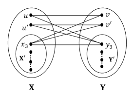
Figure 2: Graph $G$

Since $G$ is connected, so at least one of the vertices of $u$ or $v$ is adjacent with the vertices in $Y^{{}^{\prime}}$ or $X^{{}^{\prime}}$, respectively. Without loss of generalities, let us assume that $u\sim y$ for some $y\in Y^{{}^{\prime}}$. Now, every vertex of $X^{{}^{\prime}}$ is adjacent with $v$. Otherwise, there is a vertex $x\in X^{{}^{\prime}}$ such that $x\nsim v$. Then the induced underlying subgraph $H_{1}$(say) formed by the vertices $\{u,v,y,x\}$ is isomorphic to $P_{4}$ and $\mu(G)=\mu(H_{1})+\mu(G-H_{1})$. Therefore, by Lemma 4.6, $\mathcal{E}(\Phi)>2\mu(G)$, a contradiction. Thus every vertex in $X^{{}^{\prime}}$ is adjacent with $v$.

Suppose $u$ is not adjacent to some of the vertices of $Y^{{}^{\prime}}$. Let $y_{1}\in Y^{{}^{\prime}}$ such that $y_{1}\nsim u$. Let $x_{1}\in X^{{}^{\prime}}$. Then the induced subgraph formed by the vertices $\{y_{1},x_{1},u,v\}$ is isomorphic to $P_{4}$. Then by an argument similar to above, we can show that $\mathcal{E}(\Phi)>2\mu(G)$. Again we get a contradiction. Therefore, $X^{{}^{\prime}}\subset N(v)$ and $Y^{{}^{\prime}}\subset N(u)$. Consider $x_{3}\in X^{{}^{\prime}}$ and $y_{3}\in Y^{{}^{\prime}}$. Take the induced subgraph $H_{2}$ formed by the vertices $\{u,v,u^{{}^{\prime}},v^{{}^{\prime}},x_{3},y_{3}\}$ which is given in the Figure 2 and of the form shown in Figure 1. Then $\mu(G)=\mu(H_{2})+\mu(G-H_{2})$. Also by the Lemma 4.7, $\mathcal{E}((H_{2},\varphi))>2\mu(H_{2})$. Therefore, by the Lemma 4.6, $\mathcal{E}(\Phi)>2\mu(G)$. Which is a contradiction. Thus $N(u)=Y$. Therefore, $G=K_{\frac{n}{2},\frac{n}{2}}$.

Claim 2: $\varphi=1.$
Since $G=K_{\frac{n}{2},\frac{n}{2}}$, so $\mu(G)=\frac{n}{2}$. Then $\Phi=(K_{\frac{n}{2},\frac{n}{2}},\varphi)$ with $\mathcal{E}(\Phi)=n=\mathcal{E}(K_{\frac{n}{2},\frac{n}{2}})$. Therefore, by the Theorem 3.3, $\Phi\sim(K_{\frac{n}{2},\frac{n}{2}},1)$. ∎

A k-walk (or simply walk) in an undirected graph $G$ with vertex set $V(G)=\{v_{1},v_{2},\dots,v_{s}\}$ is an alternative sequence of vertices and edges. We simply denote $v_{i_{1}}-v_{i_{2}}-\cdots-v_{i_{r}}$ as a $r$-walk from the vertex $v_{i_{1}}$ to $v_{i_{r}}$, where the vertices and edges in this walk may or may not be distinct. We call a walk $v_{i_{1}}-v_{i_{2}}-\cdots-v_{i_{r}}$, a path if all the edges in this walk are distinct. If there is a path in between the vertices $v_{x}$ and $v_{y}$, then we call $v_{x}$ and $v_{y}$ is connected and denoted by $v_{x}\leftrightarrow v_{y}$.

Let $G_{1}$ and $G_{2}$ be two undirected graph with $V(G_{1})=\{v_{1},v_{2},\dots,v_{s}\}$ and $V(G_{2})=\{u_{1},u_{2},\dots,u_{t}\}$. To avoid the confusion, in definition of Kronecker product, we use the following notation. If $v_{i}\sim v_{j}$, then the undirected edge in between them is denoted by $v_{i}v_{j}$ and the oriented edge from the vertex $v_{i}$ to $v_{j}$ is denoted by $(\overrightarrow{v_{i}v_{j}})$. Let $\Phi=(G_{1},\varphi)$ be any $\mathbb{T}$-gain graph. A $\mathbb{T}$-gain Kronecker product of $\Phi$ and a simple graph $G_{2}$ is defined as a $\mathbb{T}$-gain graph, $\Phi\otimes G_{2}=(G_{1}\otimes G_{2},\psi)$ on an underlying graph $G_{1}\otimes G_{2}$ with vertex set $V(G_{1}\otimes G_{2})=\{(v_{p},u_{q}):p=1,2,\dots,s\text{, and }q=1,2,\dots,t\}$ and edge set $E(G_{1}\otimes G_{2})=\{(v_{p},u_{q})(v_{a},u_{b}):v_{p}\sim v_{a}\text{ and }u_{q}\sim u_{b}\}$ such that $\psi(\overrightarrow{(v_{p},u_{q})(v_{a},u_{b})})=\varphi(\overrightarrow{v_{p}v_{a}})$. The $\mathbb{T}$-gain graph $\Phi\otimes K_{2}$ is called $\mathbb{T}$-gain bipartite double, where $K_{2}$ is a complete graph of $2$ vertices. We illustrate the following example of a $\mathbb{T}$-gain bipartite double.

Example 4.1.

Let $G$ be a triangle with vertex set $V(G)=\{v_{1},v_{2},v_{3}\}$ and $V(K_{2})=\{x,y\}$. Let $\Phi=(G,\varphi)$ be a $\mathbb{T}$-gain graph. Then $\Phi\otimes K_{2}$ is a $\mathbb{T}$-gain bipartite double. See Figure 3.

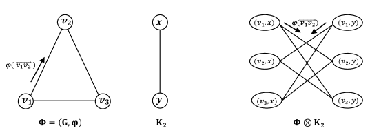
Figure 3: $\mathbb{T}$-gain bipartite double of $\Phi$ and $K_{2}$

For any two matrices $P=(p_{ij})_{r_{1}\times r_{2}}$ and $Q=(q_{st})_{s_{1}\times s_{2}}$, the Kronecker product of the matrices $P$ and $Q$ are defined as $P\otimes Q=(p_{ij}Q)_{r_{1}s_{1}\times r_{2}s_{2}}$. Now, it is easy to see that $A(\Phi\otimes G_{2})=A(\Phi)\otimes A(G_{2})$.

The following lemma is an extension of Lemma 2.6 for the $\mathbb{T}$-gain graphs.

Lemma 4.8.

Let $\Phi\otimes G$ be a $\mathbb{T}$-gain Kronecker product of a $\mathbb{T}$-gain graph $\Phi=(G_{1},\varphi)$ and an undirected graph $G$. If $\operatorname{spec}(\Phi)=\{\lambda_{1},\lambda_{2},\dots,\lambda_{s}\}$ and $\operatorname{spec}(G)=\{\gamma_{1},\gamma_{2},\dots,\gamma_{t}\}$. Then $\operatorname{spec}(\Phi\otimes G)=\{\lambda_{i}\gamma_{j}:i=1,2,\dots,s,j=1,2,\dots,t\}$.

The following lemma is an extension of Lemma 2.8 for the $\mathbb{T}$-gain graphs.

Lemma 4.9.

If $\Phi=(G,\varphi)$ be any connected $\mathbb{T}$-gain graph on a non bipartite graph $G$, then $\mathcal{E}(\Phi)>2\mu(G)$.

Proof.

Let $\Phi=(G,\varphi)$ be a connected $\mathbb{T}$-gain graph on a non bipartite graph $G$ with vertex set $V(G)=\{v_{1},v_{2},\dots,v_{n}\}$ and $m$ edges. If possible let $\mathcal{E}(\Phi)=2\mu(G)$. Then, by Lemma 4.4, $G$ has perfect matching, say $M$. Let $v_{i}v_{j}$ denote the edge between the vertices $v_{i}$ and $v_{j}$, if it exists. Let $M=\{v_{1}v_{2},v_{3}v_{4},\dots,v_{n-1}v_{n}\}$ be a perfect matching in $G$. Then $\mu(G)=|M|=\frac{n}{2}$. Therefore, $\mathcal{E}(\Phi)=2\mu(G)=n$. Let $V(K_{2})=\{x,y\}$. Now we consider a $\mathbb{T}$-gain Kronecker product $\Phi\otimes K_{2}$. Then $|V(\Phi\otimes K_{2})|=2n$ and $|E(\Phi\otimes K_{2})|=2m$. It is easy to see that $\Phi\otimes K_{2}$ is a bipartite graph with a perfect matching $\{(v_{1},x)(v_{2},y),(v_{1},y)(v_{2},x),\dots,(v_{n-1},x)(v_{n},y),(v_{n-1},y)(v_{n},x)\}$. Then $\mu(\Phi\otimes K_{2})=n$. Now, by Lemma 4.8, $\mathcal{E}(\Phi\otimes K_{2})=2\mathcal{E}(\Phi)=2n=2\mu(\Phi\otimes K_{2})$. That is, $\mathcal{E}(\Phi\otimes K_{2})=2\mu(\Phi\otimes K_{2})$.
Claim: $\Phi\otimes K_{2}$ is connected.
The vertex set of $\Phi\otimes K_{2}$ is $V(\Phi\otimes K_{2})=\{(v_{1},x),(v_{2},x),\dots,(v_{n},x),(v_{1},y),(v_{2},y),\dots,(v_{n},y)\}$. Since $G$ is connected, so for any pair of vertices $v_{i}$ and $v_{j}$, there is a path in between them, $v_{i}=v_{i_{0}}-v_{i_{1}}-\cdots-v_{i_{t}}=v_{j}$, (say). Now $v_{i}$ and $v_{j}$ is corresponds with the four vertices, $S=\{(v_{i},x),(v_{i},y),(v_{j},x),(v_{j},y)\}$ in $V(\Phi\otimes K_{2})$. We show that any pair of two vertices in that four vertices set is connected. If $t$ is even, then we have two paths in $(\Phi\otimes K_{2})$, $(v_{i},x)=(v_{i_{0}},x)-(v_{i_{1}},y)-\cdots-(v_{i_{t}},x)=(v_{j},x)$ and $(v_{i},y)=(v_{i_{0}},y)-(v_{i_{1}},x)-\cdots-(v_{i_{t}},y)=(v_{j},y)$. Thus $(v_{i},x)\leftrightarrow(v_{j},x)$ and $(v_{i},y)\leftrightarrow(v_{j},y)$. If $t$ is odd then similarly, $(v_{i},x)\leftrightarrow(v_{j},y)$ and $(v_{i},y)\leftrightarrow(v_{j},x)$. Therefore, it is enough to show that $(v_{i},x)\leftrightarrow(v_{i},y)$. Since $G$ is connected non bipartite graph, so we can always find a walk from $v_{i}$ to $v_{i}$ of odd length (walk travels an odd cycle). Then similar to above, $(v_{i},x)\leftrightarrow(v_{i},y)$. Therefore, $(v_{i},x)$ is connected with other three vertices of $S$. Since $v_{i}$ and $v_{j}$ are arbitrary pair of vertices of $G$, so any two vertices of $\Phi\otimes K_{2}$ are connected. Thus $\Phi\otimes K_{2}$ is connected.

Since $\Phi\otimes K_{2}$ is a connected bipartite $\mathbb{T}$-gain graph of $2n$ vertices with $\mathcal{E}(\Phi\otimes K_{2})=2\mu(\Phi\otimes K_{2})$, so by Lemma 4.8, $\Phi\otimes K_{2}\sim(K_{n,n},1)$. Thus $2m=|K_{n,n}|=n^{2}$. That is, $|E(G)|=m=\frac{n^{2}}{2}>\frac{n(n-1)}{2}=|E(K_{n})|$. Which is a contradiction. Hence the result. ∎

Lemma 4.10.

Let $\Phi=(G,\varphi)$ be any connected $\mathbb{T}$-gain graph on $n$ vertices with the matching number $\mu(G)$. If $\mathcal{E}(\Phi)=2\mu(G)$, then $\Phi\sim(K_{\frac{n}{2},\frac{n}{2}},1)$.

Proof.

Since $\mathcal{E}(\Phi)=2\mu(G)$, so by the Lemma 4.9, $G$ must be bipartite. Therefore, $\Phi=(G,\varphi)$ is a connected bipartite $\mathbb{T}$-gain graph. Now, applying the Theorem 4.6 we have $\Phi\sim(K_{\frac{n}{2},\frac{n}{2}},1)$. ∎

Let $A_{1},A_{2},\dots,A_{t}$ be $t$ square complex matrices. Then we denote $A_{1}\oplus A_{2}\oplus\cdots\oplus A_{t}$ as a block diagonal matrix with diagonal blocks are $A_{1},A_{2},\dots,A_{t}$. That is, $\bigoplus\limits_{j=1}^{t}A_{j}=diag(A_{1},A_{2},\dots,A_{t})$.

In the next theorem, we characterize the class of $\mathbb{T}$- gain graphs for which equality holds in Theorem 4.5.

Theorem 4.7.

Let $\Phi=(G,\varphi)$ be any $\mathbb{T}$-gain graph with matching number $\mu(G)$. Then $\mathcal{E}(\Phi)=2\mu(G)$ if and only if each component of $\Phi$ is a balanced complete bipartite $\mathbb{T}$-gain graph with a perfect matching together with some isolated vertices.

Proof.

Let $G_{1},G_{2},\dots,G_{p},G_{p+1},\dots,G_{p+r}$ be the connected components of $G$. Without loss of generality, let us assume that the last $r$ components are the only isolated vertices. Then $\mu(G)=\mu(G_{1})+\dots+\mu(G_{p})$. It is clear that $A(\Phi)=\bigoplus\limits_{j=1}^{p+r}A((G_{j},\varphi))$ , So $\mathcal{E}(\Phi)=\sum\limits_{j=1}^{p}\mathcal{E}((G_{j},\varphi))$. Therefore, by the Theorem 4.5, we have,

$$2\mu(G)=\mathcal{E}(\Phi)=\sum\limits_{j=1}^{p}\mathcal{E}((G_{j},\varphi))\geq 2\sum\limits_{j=1}^{p}\mu(G_{j})=2\mu(G)$$ (13)

Thus $\mathcal{E}((G_{j},\varphi))=2\mu(G_{j})$, for each $j=1,2,\dots,s$. Now, using the Lemma 4.10, we can derive the result. ∎

As an application of the above theorem, we can establish a relationship among the energy of $\mathbb{T}$-gain graph, the vertex cover number and the number of odd cycles. This result generalizes one of the main results of [16]. Let $\Phi=(G,\varphi)$ be a $\mathbb{T}$-gain graph with vertex set $V(G)$. Let $u\in V(G)$. Then $(\Phi-u)$ denotes an induced subgraph of $\Phi$ with vertex set $V(G)\setminus\{u\}$.

Theorem 4.8.

Let $\Phi=(G,\varphi)$ be any $\mathbb{T}$-gain graph on $G$ with $c(G)$ number of odd cycles and vertex cover number $\tau(G)$. Then

$$\mathcal{E}(\Phi)\geq 2\tau(G)-2c(G).$$

Equality occurs if and only if each component of $\Phi$ is a balanced complete bipartite $\mathbb{T}$-gain graph with a perfect matching together with some isolated vertices.

Proof.

Let $\Phi=(G,\varphi)$ be any $\mathbb{T}$-gain graph with $c(G)$ number of odd cycles. Let us prove the bound using induction on the number of odd cycles $c(G)$. If $c(G)=0$, then $G$ is bipartite. Therefore $\mu(G)=\tau(G)$. Now, by Theorem 4.5, we have $\mathcal{E}(\Phi)\geq 2\mu(G)=2\tau(G)-2c(G)$. Assume that the statement is true for any $\mathbb{T}$-gain graph with the number of odd cycles is at most $(c(G)-1)$. Consider $\Phi$ with $c(G)\geq 1$ number of odd cycles. Let $u$ be a vertex in an odd cycle of $G$. Then the number of odd cycles, say $c^{{}^{\prime}}$, of $\Phi-u$ is at most $(c(G)-1)$. Thus, by induction hypothesis, $\mathcal{E}(\Phi-u)\geq 2\tau(G-u)-2c^{{}^{\prime}}$. Since $u$ is an isolated vertex, so, by Lemma 4.3, $\mathcal{E}(\Phi)>\mathcal{E}(\Phi-u)$.

It is easy to see that $\tau(G-u)\geq\tau(G)-1$. Therefore, $\mathcal{E}(\Phi)>\mathcal{E}(\Phi-u)\geq 2\tau(G)-2c(G)$.

Now, let $\mathcal{E}(\Phi)=2\tau(G)-2c(G)$. If $c(G)\geq 1$, then, by the above observation, $\mathcal{E}(\Phi)>2\tau(G)-2c(G)$. which is a contradiction. That is $c(G)=0$. Therefore, $G$ is bipartite and $\mu(G)=\tau(G)$. Thus $\mathcal{E}(\Phi)=2\mu(G)$. Now, by Theorem 4.6, $\Phi$ is the disjoint union of some balanced complete bipartite $\mathbb{T}$-gain graphs with a perfect matching together with some isolated vertices. ∎

5 Upper bound of energy of $\mathbb{T}$-gain graph in terms of vertex cover number and largest vertex degree

In this section, our main objective is to obtain an upper bound for the energy of a $\mathbb{T}$-gain graph in terms of the vertex cover number and the largest vertex degree. This result is the counter part of the corresponding known result about undirected graph [Theorem 1.3] and mixed graph [Theorem 1.4]. Furthermore, we characterize all $\mathbb{T}$-gain graphs for which the upper bound is attained. This characterization completely solve one of the open problem [16].

Theorem 5.1.

Let $\Phi=(G,\varphi)$ be any $\mathbb{T}$-gain graph with the vertex cover number $\tau(G)$, and maximum vertex degree $\Delta(G)$. Then,

$$\mathcal{E}(\Phi)\leq 2\tau(G)\sqrt{\Delta(G)}.$$ (14)

Proof.

Let $\Phi=(G,\varphi)$ be any $\mathbb{T}$-gain graph with vertex cover number $\tau(G)$. We prove the result by induction on $\tau(G)$. If $\tau(G)=1$, then $G$ must be $K_{1,r}$, for some $r$ together with some isolated vertices. Therefore, $\Phi$ is balanced. Now $\mathcal{E}(\Phi)=\mathcal{E}(K_{1,r})=2\sqrt{r}=2\tau(G)\sqrt{\Delta(K_{1,r})}$.

Let us assume that for any $\mathbb{T}$-gain graph $\Psi=(G_{1},\psi)$ with $\tau(G_{1})<\tau(G)$, we have $\mathcal{E}(\Psi)\leq 2\tau(G_{1})\sqrt{\Delta(G_{1})}$. Let $U$ be a minimum vertex cover of $G$. Then $|U|=\tau(G)\geq 2$. Let $x\in U$. Let $S$ be an induced subgraph of $G$ which is formed by removing the vertex $x$, and the edges incident with $x$ from $G$. That is $S=G-x$. Then $\tau(S)=\tau(G)-1$. Therefore, by the induction hypothesis, $\mathcal{E}(\Phi-x)=\mathcal{E}((S,\varphi))\leq 2\tau(S)\sqrt{\Delta(S)}$. After a suitable relabeling of vertices, we can express $A(\Phi)$ as

$$A(\Phi)=\left[\begin{array}[]{ccc}0&{\textbf{v}^{*}}&{\textbf{0}}\\ {\textbf{v}}&A_{1}&Y^{*}\\ {\textbf{0}}&Y&A_{2}\end{array}\right]=\left[\begin{array}[]{ccc}0&{\textbf{v}^{*}}&{\textbf{0}}\\ {\textbf{v}}&{\textbf{0}}&{\textbf{0}}\\ {\textbf{0}}&{\textbf{0}}&{\textbf{0}}\end{array}\right]+\left[\begin{array}[]{ccc}0&{\textbf{0}}&{\textbf{0}}\\ {\textbf{0}}&A_{1}&Y^{*}\\ {\textbf{0}}&Y&A_{2}\end{array}\right]$$

Here the first column and the first row are associated with the vertex $x$. Let the degree of $x$ be $d$. Then $\left[\begin{array}[]{cc}0&{\textbf{v}^{*}}\\ {\textbf{v}}&{\textbf{0}}\end{array}\right]$ and $\left[\begin{array}[]{cc}A_{1}&Y^{*}\\ Y&A_{2}\end{array}\right]$ are the adjacency matrices of the $\mathbb{T}$-gain subgraphs $(K_{1,d},\varphi)$ and $(S,\varphi)$, respectively. By Theorem 2.11, we have

$$\mathcal{E}(\Phi)\leq\mathcal{E}(K_{1,d})+\mathcal{E}((S,\varphi))\leq 2\sqrt{d}+2\tau(S)\sqrt{\Delta(S)}\leq 2\tau(G)\sqrt{\Delta(G)}.$$ (15)

∎

Theorem 5.2.

Let $\Phi=(G,\varphi)$ be any $\mathbb{T}$-gain graph on $G$ with vertex cover number $\tau(G)$ and maximum vertex degree $\Delta(G)$. Then

$$\mathcal{E}(\Phi)=2\tau(G)\sqrt{\Delta(G)}$$ (16)

if and only if $\Phi$ is the disjoint union of $\tau(G)$ copies of balanced $\mathbb{T}$-gain graph $(K_{1,\Delta(G)},1)$ together with some isolated vertices.

Proof.

First let us show that all the vertices of $U$ have the same vertex degree, $\Delta(G).$ Let $x\in U$ be any vertex in $U$ (as in Theorem 5.1). Since $\mathcal{E}(\Phi)=2\tau(G)\sqrt{\Delta(G)}$, so all the inequalities of (15) become equations. So $\mathcal{E}((S,\varphi))=2\tau(S)\sqrt{\Delta(S)}$, and $d=\Delta(S)=\Delta(G)$. As $x$ is arbitrary, so all the vertices of $U$ are of degree $\Delta(G)$.
Now we claim that the underlying graph $G$ is bipartite. Let $W=V(G)\setminus U$. It is clear that $U\setminus\{x\}$ is a minimum vertex cover of the induced subgraph $S$. Also, we have $\mathcal{E}((S,\varphi))=2\tau(S)\sqrt{\Delta(S)}$. Now, applying the argument

to $S$. Therefore, all the vertices of $U\setminus\{x\}$ in $S$ is of degree $\Delta(S)$. Also we know that $\Delta(S)=\Delta(G)$. Since $d=\Delta(G)$, so there is no edge between the vertex $x$ and the vertices of $U\setminus\{x\}$. As $x$ is arbitrary, so we get no two vertices of $U$ are adjacent. Now $U$ is a minimum vertex cover of $G$, so no two vertices of $W$ are adjacent. Hence $G$ is a bipartite graph with vertex partition sets $U$ and $W$.

Let $G_{1},G_{2},\dots,G_{p}$ be the only nontrivial components of $G$ (That is components contain at least one edge). Then,

$$2\tau(G)\sqrt{\Delta(G)}=\mathcal{E}(\Phi)=\sum\limits_{j=1}^{p}\mathcal{E}((G_{j},\varphi))\leq\sum\limits_{j=1}^{p}2\tau(G_{j})\sqrt{\Delta(G_{j})}\leq 2\tau(G)\sqrt{\Delta(G)}.$$

From the above expression, we get $\mathcal{E}((G_{j},\varphi))=2\tau(G_{j})\sqrt{\Delta(G_{j})}$ and $\Delta(G_{j})=\Delta(G)$, for $j=1,2,\dots,p$.

Now let us show that the rank of each component $(G_{j},\varphi)$ is $2$. Let $r_{j}$ be the rank of $(G_{j},\varphi)$. Since $(G_{j},\varphi)$ is bipartite, so its spectrum is symmetric with respect to origin. Thus $r_{j}$ is an even number and $r_{j}\geq 2$. Let $\lambda_{1}\geq\lambda_{2}\geq\cdots\geq\lambda_{r_{j}}$ be the nonzero eigenvalues of $(G_{j},\varphi).$ Suppose that $r_{j}>2$. Then $\lambda_{1}>\lambda_{2}>0$. Therefore, by the Cauchy-Schwartz inequality

$$\mathcal{E}((G_{j},\varphi))=\sum\limits_{t=1}^{j}|\lambda_{t}|<\sqrt{r_{j}}\sqrt{\sum\limits_{t=1}^{j}\lambda_{t}^{2}}=\sqrt{2|E(G_{j})|r_{j}}.$$

For any $\mathbb{T}$-gain graph $\Psi=(B,\psi)$ on a bipartite graph $B$, we know that $|E(B)|\leq\tau(B)\Delta(B)$. By Lemma 2.3, we have $\operatorname{rank}(\Psi)\leq 2\mu(B)=2\tau(B)$. Hence $\mathcal{E}((G_{j},\varphi))<2\tau(G_{j})\sqrt{\Delta(G_{j})}$, a contradiction (as for each component, $\mathcal{E}((G_{j},\varphi))=2\tau(G_{j})\sqrt{\Delta(G_{j})}$). Hence the rank of $(G_{j},\varphi)$ is $2$ for $j=1,2,\cdots,p$.

Since each nontrivial component $(G_{j},\varphi)$ is bipartite and of rank $2$. Now $(G_{j},\varphi)$ is of rank $2$ if and only if it has exactly one positive eigenvalue. Therefore, by Lemma 4.2, $(G_{j},\varphi)\sim(K_{a,b},1)$. Without loss of generality, consider $a\leq b$. Then $\tau(G_{j})=a$ and $\Delta(G_{j})=b$. Now $\mathcal{E}((G_{j},\varphi))=2\tau(G_{j})\sqrt{\Delta(G_{j})}=2\tau(G_{j})\sqrt{\Delta(G_{j})}=2a\sqrt{b}$. On the other hand $\mathcal{E}((G_{j},\varphi))=\mathcal{E}((K_{a,b},1))=2\sqrt{ab}$. Thus $2a\sqrt{b}=2\sqrt{ab}$. Thus $a=1$, and hence $b=\Delta(G_{j})=\Delta(G)$. Therefore, for each $j=1,2,\dots,p$, $(G_{j},\varphi)\sim(K_{1,\Delta(G)},1)$. ∎

References

- [1] Octavio Arizmendi, Jorge Fernandez Hidalgo, and Oliver Juarez-Romero, Energy of a vertex, Linear Algebra Appl. 557 (2018), 464–495. MR 3848283
- [2] Che-Man Cheng, Roger A. Horn, and Chi-Kwong Li, Inequalities and equalities for the cartesian decomposition of complex matrices, Linear Algebra and its Applications 341 (2002), no. 1, 219 – 237, Special issue dedicated to Professor T. Ando.
- [3] Jane Day and Wasin So, Graph energy change due to edge deletion, Linear Algebra and its Applications 428 (2008), no. 8, 2070 – 2078.
- [4] Krystal Guo and Bojan Mohar, Hermitian adjacency matrix of digraphs and mixed graphs, J. Graph Theory 85 (2017), no. 1, 217–248. MR 3634484
- [5] I. Gutman, S.Z. Firoozabadi, J.A. De La Peña, and J. Rada, On the energy of regular graphs, Match 57 (2007), no. 2, 435–442, cited By 50.
- [6] Shengjie He, Rong-Xia Hao, and Fengming Dong, The rank of a complex unit gain graph in terms of the matching number, Linear Algebra and its Applications 589 (2020), 158 – 185.
- [7] Roger A. Horn and Charles R. Johnson, Matrix analysis, second ed., Cambridge University Press, Cambridge, 2013. MR 2978290
- [8] Yuxuan Li, Lower bound of the energy of a complex unit gain graph in terms of the matching number of its underlying graph, arXiv preprint arXiv:2005.01998 [math.CO] (2020).
- [9] Jianxi Liu and Xueliang Li, Hermitian-adjacency matrices and Hermitian energies of mixed graphs, Linear Algebra Appl. 466 (2015), 182–207. MR 3278246
- [10] Ranjit Mehatari, M Rajesh Kannan, and Aniruddha Samanta, On the adjacency matrix of complex unit gain graph, arXiv preprint arXiv:1812.03747 [math.CO] (2018).
- [11] Nathan Reff, Spectral properties of complex unit gain graphs, Linear Algebra Appl. 436 (2012), no. 9, 3165–3176. MR 2900705
- [12] , Oriented gain graphs, line graphs and eigenvalues, Linear Algebra Appl. 506 (2016), 316–328. MR 3530682
- [13] Aniruddha Samanta and M. Rajesh Kannan, On the spectrum of complex unit gain graph, arXiv preprint arXiv:1908.10668 (2019).
- [14] Fenglei Tian and Dein Wong, Relation between the skew energy of an oriented graph and its matching number, Discrete Applied Mathematics 222 (2017), 179 – 184.
- [15] Long Wang and Xiaobin Ma, Bounds of graph energy in terms of vertex cover number, Linear Algebra Appl. 517 (2017), 207–216. MR 3592020
- [16] W. Wei and S. Li, Relation between the hermitian energy of a mixed graph and the matching number of its underlying graph, Linear and Multilinear Algebra (2018), cited By 1; Article in Press.
- [17] Dein Wong, Xinlei Wang, and Rui Chu, Lower bounds of graph energy in terms of matching number, Linear Algebra and its Applications 549 (2018), 276 – 286.
- [18] Thomas Zaslavsky, Signed graphs, Discrete Appl. Math. 4 (1982), no. 1, 47–74. MR 676405