Decoder Modulation for Indoor Depth Completion

Abstract

Depth completion recovers a dense depth map from sensor measurements. Current methods are mostly tailored for very sparse depth measurements from LiDARs in outdoor settings, while for indoor scenes Time-of-Flight (ToF) or structured light sensors are mostly used. These sensors provide semi-dense maps, with dense measurements in some regions and almost empty in others. We propose a new model that takes into account the statistical difference between such regions. Our main contribution is a new decoder modulation branch added to the encoder-decoder architecture. The encoder extracts features from the concatenated RGB image and raw depth. Given the mask of missing values as input, the proposed modulation branch controls the decoding of a dense depth map from these features differently for different regions. This is implemented by modifying the spatial distribution of output signals inside the decoder via Spatially-Adaptive Denormalization (SPADE) blocks. Our second contribution is a novel training strategy that allows us to train on a semi-dense sensor data when the ground truth depth map is not available. Our model achieves the state of the art results on indoor Matterport3D dataset [4]. Being designed for semi-dense input depth, our model is still competitive with LiDAR-oriented approaches on the KITTI dataset [42]. Our training strategy significantly improves prediction quality with no dense ground truth available, as validated on the NYUv2 dataset [29].

1 Introduction

In recent years, depth sensors have become an essential component of many devices, from self-driving cars to smartphones. However, the quality of modern depth sensors is still far from perfect. LiDAR systems provide accurate but spatially sparse measurements while being quite expensive and large. Commodity-grade depth sensors based on the active stereo with structured light (, Microsoft Kinect) or Time-of-Flight (, Microsoft Kinect Azure or depth sensors in many smartphones) provide estimations that are relatively dense but less accurate and within a limited distance range. LiDAR-based sensors are widely used in outdoor environments, especially for self-driving cars, while the other sensors are mainly applicable in an indoor setting. Due to the rapid growth of the self-driving car industry, the majority of recent depth completion methods are mostly focused on outdoor depth completion for LiDAR data [42, 41, 8], often overlooking other types of sensors and scenarios. Nevertheless, these sensors are an essential part of many modern devices (such as mobile phones, AR glasses, and others).

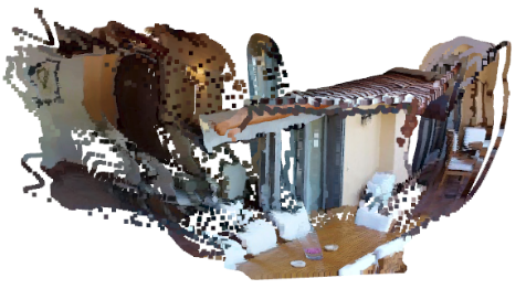
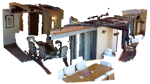
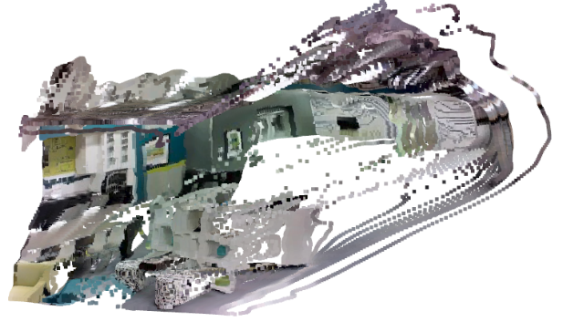
Figure 1: Point clouds are reconstructed from depth maps predicted by our model (top row) and ground truth (bottom row) taken from the Matterport3D [4] test subset.

LiDAR-oriented methods mainly deal with sparse measurements. Applying these methods to depth data captured with semi-dense sensors as-is may be a suboptimal strategy. This kind of transfer requires additional heuristics such as sparse random sampling. The most popular approach [41, 35, 9, 28] of training LiDAR-oriented methods on a semi-dense depth map proceeds as follows. First, the gaps in semi-dense depth maps are filled using simple interpolation methods such as bilateral filtering or the approach of [20]. Then, some depth points are uniformly sampled from the resulting map. This heuristic approach is used due to the lack of LiDAR data for indoor environments, but such kind of preprocessing suggests that it may be better to use a model originally designed to operate with semi-dense data. Such an approach would take into account the features of semi-dense sensor data and would not require separate heuristics for transfer.

Inspired by these observations, we present a novel solution for the indoor depth completion from semi-dense depth maps guided by color images. Since sensor data may be present for 60% of pixels and more, we propose to use a single encoder for the joint RGBD signal. Taking into account the statistical differences between regions with and without depth measurements, we design a decoder modulation branch that takes a mask as input and modifies the distributions of activation maps in the decoder. This modulation mechanism is based on Spatially-Adaptive Denormalization (SPADE) blocks [32]. Since there are few publicly available datasets with both sensor and dense ground truth depth, we additionally propose a special training strategy for depth completion models that emulates semi-dense sensors and does not require dense depth reconstruction.

As a result, we offer the following contributions:

• a novel network architecture for indoor depth completion with a decoder modulation branch;

• a novel training strategy that emulates semi-dense sensors and does not require dense depth reconstruction;

• large-scale experimental validation on real datasets including Matterport3D, ScanNet, NYUv2, and KITTI.

The paper is organized as follows. In Section 2, we review related work on depth estimation and dense image labeling. Section 3 presents our approach, including the new architecture and training strategies. Section 4 describes the experimental setup, Section 5 presents the results of our experiments, and Section 6 concludes the paper.

2 Related work

In this section, we review works on several topics related to depth processing for images or works that have served as the original inspiration for our work. Namely, we cover depth estimation, depth completion, and semantic segmentation, a well-studied case of dense image labeling.

Depth Estimation.

Methods for single view depth estimation based on deep neural networks have significantly evolved in recent years, by now rapidly approaching the accuracy of depth sensors [3, 13, 24, 27]; some of these methods are able to run in real-time [46] or even on embedded platforms [1]. However, the acquisition of accurate ground truth depth maps is complicated due to certain limitations of existing depth sensors. To overcome these difficulties, various approaches focusing on data acquisition, data refinement, and the use of additional alternative data sources have been proposed [23, 18]. We also note several recently developed weakly supervised and unsupervised approaches [36, 14].

Depth Completion.

Pioneering works on depth completion adopted complicated heuristic algorithms for processing raw sensor data. These algorithms were based on compressed sensing [15] or used a combined wavelet-contourlet dictionary [26]. Uhrig et al. [42] were the first to present a successful learnable depth completion method based on convolutional neural networks, developing special sparsity-invariant convolutions to handle sparse inputs. Learnable methods were further improved by image guidance [8, 43, 48, 39]. Tang et al. [41] proposed an approach to train content-dependent and spatially-variant kernels for sparse depth features processing. Li et al. [22] suggested a multi-scale guided cascade hourglass architecture for depth completion. Chen et al. [7] presented a 2D-3D fusion pipeline based on continuous convolutions. Apart from utilizing images, some recently proposed methods make use of surface normals [35, 16, 47, 50] and object boundaries [16, 50].

Most of the above-mentioned works focus on LiDAR-based sparse depth completion in outdoor scenarios and report results on the well-known KITTI benchmark [42]. There are only a few works that consider processing non-LiDAR semi-dense depth data obtained with Kinect sensors. Recently, Zhang et al. [50] introduced Matterport3D, a large-scale RGBD dataset for indoor depth completion, and used it to showcase a custom depth completion method. This method implicitly exploits extra data by using pretrained networks for normal estimation and boundary detection, and the resulting normals and boundaries are used in global optimization. Overall, the complexity of this method strictly limits its practical usage. Huang et al. [16] was the first to outperform the original results on this dataset. Similar to Zhang et al. [50], their results were achieved via a complicated multi-stage method that involved resource-intensive preprocessing. Although it does not rely on pretrained backbones, it uses a normal estimation network explicitly trained on external data. In this work, we propose a novel depth completion method that presents strong baseline results while being scalable and straightforward.

Semantic segmentation and dense labeling.

Since depth completion or depth estimation can be formulated as a dense labeling problem, techniques and architectures that have proven to be effective for other dense labeling tasks might be useful for depth completion as well. Encoder-decoder architectures with skip connections originally developed for semantic segmentation [38] have shown themselves to be capable of solving a wide range of tasks. Chen et al.[5] proposed a powerful architecture based on atrous spatial pyramid pooling for semantic segmentation and improved it in further work [6]. Other important approaches include the refinement network [25] and the pyramid scene parsing network [51]. At the same time, lightweight networks such as [30] capable of running in a resource-constrained device in real-time can be of use in other deep learning-driven applications. Our depth completion network is based on the blocks proposed in [25, 31].

3 Approach and methods

Figure 2: High-level architecture of the proposed DM-LRN network. Pretrained EfficientNet [40] backbone encodes the input RGBD signal. Extracted features are fed into the lightweight RefineNet decoder [31] consisting of chained residual pooling (CRP) blocks and fusion (FUSE) blocks [31]. The decoder modulation branch modifies the spatial distribution of output signals inside the decoder via SPADE blocks [32].

Architecture overview.

The general structure of the proposed architecture is shown in Fig. 2. Our architecture design follows the standard encoder-decoder paradigm with a pretrained backbone network modified for 4D input. In our experiments, we use the EfficientNet family [40] as a backbone. The decoder part is based on a lightweight RefineNet decoder [31] combined with a custom modulation branch described below. The network takes an image, sensor depth, and a mask as input and outputs a completed depth map. No additional data is required.

Decoder Modulation Branch.

To introduce the decoder modulation branch, let us take a closer look at the forward propagation path of the network. The backbone network generates feature maps from the input RGBD signal. The input signal initially has an inhomogeneous spatial distribution, since a part of the depth data is missing. The signal compression inside a backbone smoothes this inhomogeneity, which works well for small depth gaps. If the depth gaps are too large, the convolutions generate incorrect activations due to the domain shift between RGB and RGBD signals. Aiming to reduce this domain gap, we propose to learn spatially-dependent scale and bias for normalized feature maps inside the decoder part of the architecture. This procedure is called spatially-adaptive denormalization (SPADE) and was first introduced by Park et al. [32].

Let $f^{i}_{n,c,y,x}$ denote the activation maps of the $i$th layer of the decoder for a batch of $N$ samples with shape $C_{i}\times H_{i}\times W_{i}$, and let m denote a modulation signal. The output value from SPADE $g^{i}_{n,c,y,x}$ at location $(n\in N,c\in C_{i},y\in H_{i},x\in W_{i})$ is

$$g^{i}_{n,c,y,x}=\gamma^{i}_{n,c,y,x}(\textbf{m})\frac{f^{i}_{n,c,y,x}-\mu^{i}_{c}}{\sigma^{i}_{c}}+\beta^{i}_{n,c,y,x}(\textbf{m}),$$

where $\mu^{i}_{c}=\frac{1}{N_{i}W_{i}H_{i}}\sum_{n,x,y}f^{i}_{n,c,y,x}$ is the sample mean and $\sigma^{i}_{c}=\sqrt{\frac{1}{N_{i}W_{i}H_{i}}\sum_{n,x,y}(f^{i}_{n,c,y,x}-\mu^{i}_{c})^{2}}$ is the sample (biased) standard deviation, and $\gamma^{i}_{n,c,y,x}$ and $\beta^{i}_{n,c,y,x}$ are the spatially dependent scale and bias for batch normalization respectively. In our case, the modulation signal m is the input mask of missing depth values.

Fig. 3 illustrates the decoder modulation branch in detail. This subnetwork consists of a simple mask encoder composed of convolutions with bias terms and activations and SPADE blocks that perform modulation. A bias term in the convolutions is necessary to avoid zero signals that can cover a significant part of the input mask.

(a) Decoder modulation branch.

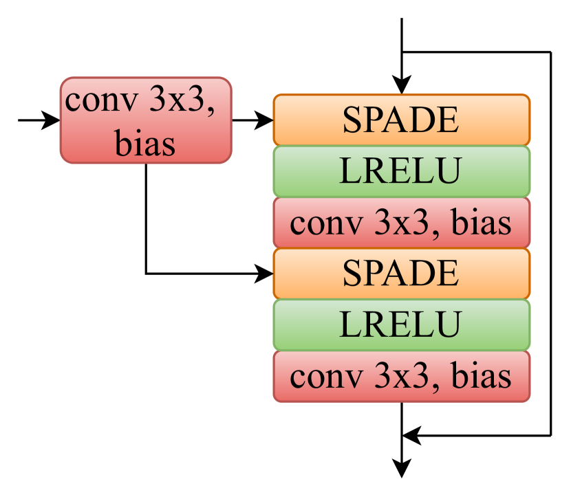
(b) SPADE.

(c) SPADE block.

Figure 3: Architecture of the decoder modulation branch (3(a)). It consists of a simple encoder composed of two biased convolutions with activations and a series of SPADE blocks (3(c)). These blocks include the SPADE layer (3(c)) that performs modulation. We use LeakyReLU activations, as the modulation should be able to decrease the scale of a signal and move it in the negative direction as well.

Training strategy.

Existing highly annotated large-scale indoor datasets do not always include both sensor depth data and ground truth depth data [49, 29], which might be an issue for the development of depth completion models. If the sensor or reconstructed depth is not available, we propose to use specially developed corruption techniques in order to obtain synthetic semi-dense sensor data.

Let $t\in T$ be a target sample that we want to degrade. Our goal is to construct a function $h:T\to S$ that transforms a depth map from the target domain $T$ to pseudo-sensor domain $S$. We assume that this procedure is sample-specific and can be factorized:

$$h(\cdot)=z_{g}(\cdot|q)\circ z_{n}(\cdot)=z_{n}(z_{g}(\cdot|q)),$$

where $q$ is the input RGB image. The term $z_{g}$ emulates a zero masking process guided by the image and $z_{n}$ is the zero masking caused by noise. The noise term $z_{n}$ represents a random spattering procedure uniformly distributed over the entire image. The specific form of $z_{g}$ may vary. Fig. 4 presents some possible approaches results. As shown in Figs. 4(d) and 4(b), the most suitable variant for semi-dense depth sensor simulation appears to be the graph-based segmentation algorithm introduced by Felzenszwalb and Huttenlocher [12], thresholded by segment area. After obtaining pseudo-sensor data, we can perform a standard training procedure on it.

Our corruption strategy (Fig. 4(d)) based on image segmentation significantly differs from widely-used sparse uniform sampling (Fig. 4(f)). Below we compare these two strategies numerically on the NYUv2 dataset [29] using our model and additional open-source approaches from the KITTI dataset leaderboard [42].

(a) RGB

(b) Initial real sensor

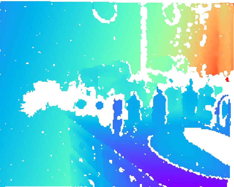
(c) Graph-based [12]

(d) Quickshift [45]

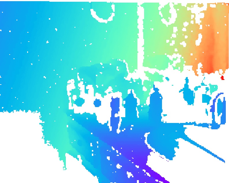
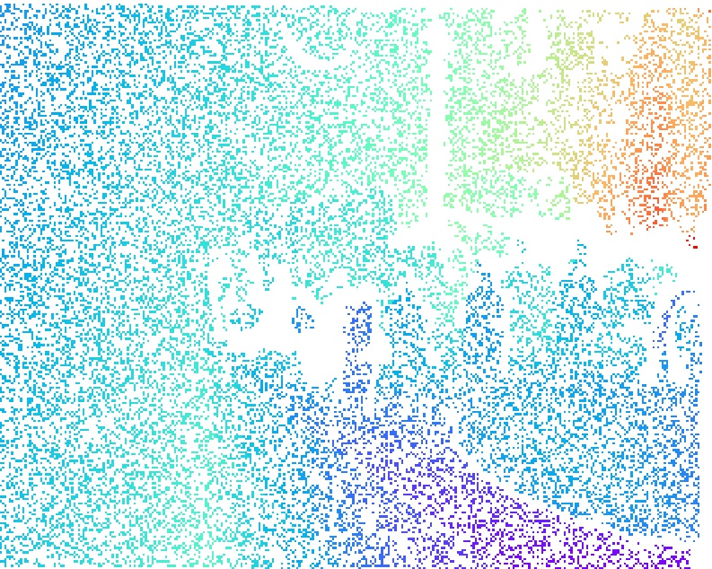
(e) Slic [2]

(f) Uniform [28]

Figure 4: Qualitative comparison of different sampling strategies based on classical image segmentation methods applied to a NYUv2 [29] sample from the raw subset: 4(b) and 4(b) – original image and depth map respectively; 4(d) – graph-based segmentation [12], 4(d) – quickshift segmentation (Vedaldi et al.[45]), 4(f) – SLIC segmentation (Achanta et al.[2]). All methods produce an image partition, then we replace depth data with zeros in segments with area below a predefined threshold value. Graph-based segmentation demonstrates the best match to the original sensor map, producing similar artifacts (diffusion on the border of the table).

Loss function.

Recent works underline two primary families of losses that are conceptually different: pixel-wise and pairwise. Pixel-wise loss functions measure the mean per-pixel distance between prediction and target, while their pairwise counterparts express the error by comparing the relationships between pairs of pixels $i$, $j$ in the output. The latter loss functions force the relationship between each pair of pixels in the prediction to be similar to that of the corresponding pair in the ground truth. In this work, we have experimented with several different single-term loss functions, including pair-wise and pixel-wise approaches in a logarithmic and actual domain (see supplementary materials for details). The logarithmic $L_{1}$ pair-wise loss function [37] appears to be the most suitable for our network. It can be expressed as

$$\mathcal{L}(y_{i},y_{i}^{*})=\frac{1}{|\mathcal{O}|^{2}}\sum_{i,j\in\mathcal{O}}\bigg{|}\log\frac{y_{i}}{y_{j}}-\log\frac{y_{i}^{*}}{y_{j}^{*}}\bigg{|},$$

where $\mathcal{O}$ is the set of pixels where the ground truth depth is non-zero, $i,j$ are pixel indices, $y_{i},y^{*}_{i}$ are the predicted and target depth respectively. Following Eigen et al. [11], our model predicts $\log y_{i}$ directly.

4 Experimental setup

RGB

Sensor

GT

Gansbeke et al.

Li et al.

Huang et al.

Ours

Figure 5: Qualitative comparison with Gansbeke et al.[44], Li et al.[21], Huang et al.[16] on Matterport3D test set. We train [44] and [21] on Matterport3D using the official code of the corresponding approaches, and results for [16] are based on the official pretrained model. Rows 2 and 4 represent zoomed-in fragments from rows 1 and 3, respectively. All images are created using color maps with the same value limits. Our model generates the completed depth map with very sharp boundaries.

	RMSE $\downarrow$	MAE $\downarrow$	$\delta_{1.05}$ $\uparrow$	$\delta_{1.10}$ $\uparrow$	$\delta_{1.25}$ $\uparrow$	$\delta_{1.25^{2}}$ $\uparrow$	$\delta_{1.25^{3}}$ $\uparrow$	SSIM $\uparrow$
Huang et al.[16]	1.092	0.342	0.661	0.750	0.850	0.911	0.936	0.799
Zhang et al.[50]	1.316	0.461	0.657	0.708	0.781	0.851	0.888	0.762
Gansbeke et al.[44]	1.161	0.395	0.542	0.657	0.799	0.887	0.927	0.700
Li et al.[21]	1.054	0.397	0.508	0.631	0.775	0.874	0.920	0.700
Gansbeke et al.[44] (ours)	1.264	0.484	0.675	0.741	0.826	0.888	0.920	0.780
Li et al.[21] (ours)	1.134	0.426	0.649	0.729	0.834	0.899	0.928	0.774
DM-LRN (ours)	0.961	0.285	0.726	0.813	0.890	0.933	0.949	0.844
LRN (ours)	1.028	0.299	0.719	0.805	0.890	0.932	0.950	0.843
LRN + mask (ours)	1.054	0.298	0.737	0.815	0.889	0.933	0.950	0.844

Table 1: Matterport3D TEST. We use the results for Huang et al.[16] and Zhang et al.[50] reported in [16]. Gansbeke et al.[44] and Li et al.[21] are trained on Matterport3D using their official implementations. Models labeled as “ours” are trained using our proposed pipeline. The two bottom rows represent models without the decoder modulation branch, with and without the mask on the input. RMSE and MAE are measured in meters.

Datasets.

We perform comparative experiments on the following datasets: Matterport3D [4], ScanNet [10], NYUv2 [29] and KITTI[42]. Matterport3D includes real sensor data and ground truth depth data obtained from official reconstructed meshes. We use it as the primary target dataset. In order to investigate the generalization capabilities of the model, we perform validation of the models trained on the Matterport3D dataset directly on ScanNet. NYUv2 does not provide dense depth reconstruction for the entire dataset, so we evaluate our training strategy on this dataset. Although our approach is not intended to be applied to sparse depth sensors, we compare it with the best performing models on the KITTI dataset.

Evaluation metrics

Following the standard evaluation protocol for indoor depth completion, we use root mean squared error (RMSE), mean absolute error (MAE), $\delta_{i}$, and SSIM. The $\delta_{i}$ metric denotes the percentage of predicted pixels where the relative error is less than a threshold $i$. Specifically, we evaluate $\delta_{i}$ for $i$ equal to $1.05$, $1.10$, $1.25$, $1.25^{2}$, and $1.25^{3}$; smaller values of $i$ correspond to making the $\delta_{i}$ metric more sensitive, while larger values reflect a more accurate prediction. RMSE and MAE directly measure absolute depth accuracy. RMSE is more sensitive to outliers than MAE and is usually chosen as the main metric for ranking models. In general, our testing pipeline for indoor depth completion is similar to Huang et al. [16].. Following the KITTI leaderboard, we evaluate RMSE, MAE, iRMSE and iMAE metrics on the KITTI dataset.

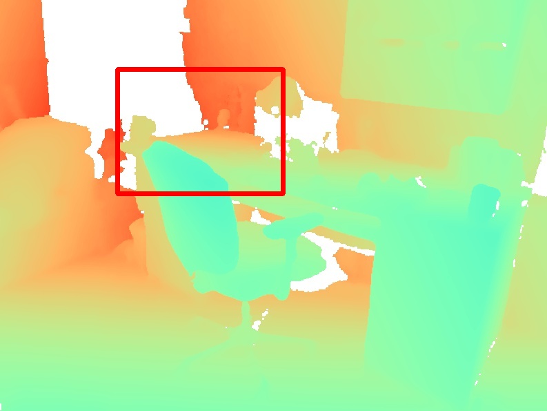
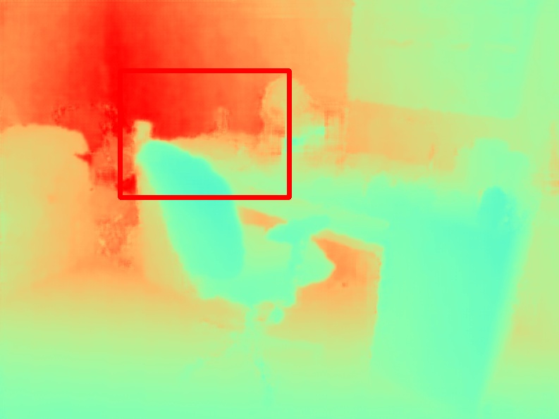
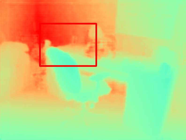
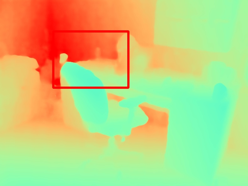
RGB

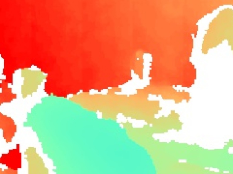
Sensor

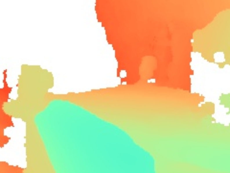
GT

Gansbeke et al.

Li et al.

Huang et al.

Ours

Figure 6: Qualitative comparison with Gansbeke et al.[44], Li et al.[21], Huang et al.[16] on ScanNet [10]. All models are trained on Matterport3D. The images are received using a unified color map.

	RMSE $\downarrow$	MAE $\downarrow$	$\delta_{1.05}$ $\uparrow$	$\delta_{1.10}$ $\uparrow$	$\delta_{1.25}$ $\uparrow$	$\delta_{1.25^{2}}$ $\uparrow$	$\delta_{1.25^{3}}$ $\uparrow$	SSIM $\uparrow$
Huang et al.[16]	0.244	0.097	0.736	0.850	0.945	0.982	0.992	0.812
Zhang et al.[50]	0.214	0.080	0.769	0.881	0.958	0.985	0.993	0.850
Gansbeke et al.[44]	0.223	0.074	0.829	0.899	0.954	0.980	0.990	0.850
Li et al.[21]	0.190	0.067	0.828	0.903	0.961	0.986	0.995	0.875
DM-LRN (ours)	0.198	0.054	0.900	0.933	0.962	0.982	0.992	0.918

Table 2: ScanNet TEST. Cross-dataset testing demonstrates the strong generalization capability of our method. All models are trained on Matterport3D. RMSE and MAE are measured in meters.

Implementation details

In our experiments, we use the Adam [17] optimizer with initial learning rate set to $10^{-4}$, $\beta_{1}=0.9$, $\beta_{2}=0.999$ and without weight decay. The pretrained EfficientNet-b4 [40] backbone is used unless otherwise stated. Batch normalization is controlled by the modulation process, so we fine-tune its parameters during the first epoch only, and afterwards these parameters are fixed. The training process is performed end-to-end for 100 epochs on a single Nvidia Tesla P40 GPU. We implement all models in Python 3.7 using the PyTorch library [33].

5 Results

Matterport3D.

We begin by inferencing our indoor pipeline on the Matterport3D dataset. Since very few previous approaches have been tested and achieved good results on this dataset, we train some of the best performing open-source KITTI models [21, 44] for a fair comparison. Assuming that the original training pipeline of these models might be designed specifically for LiDAR data, we also perform a complementary training procedure in our training setup.

The results of this quantitative comparison are presented in Table 1. Our training pipeline applied to KITTI models improves the results in terms of $\delta_{i}$, especially with smaller values of $i$, but leads to artifacts captured by RMSE values. The original training setup of these methods also does not show state of the art performance on Matterport3D (see Table 1). We use the original training procedure for further experiments. These methods do not produce sharp edges (see Fig. 5) that are crucial for indoor applications. Zhang et al. [50] and Huang et al. [16] managed to address this problem and received less blurry results. Our model produces improved completed depth while being more accurate in terms of both RMSE and MAE. In Table 1, we also present ablation experiments including different masking strategies.

A visual comparison is shown in Figure 5. Our model keeps the sensor data almost unchanged and sharp. Moreover, the geometric shapes of the interior layout and objects in the scene remain distinct.

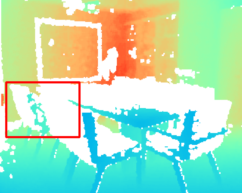
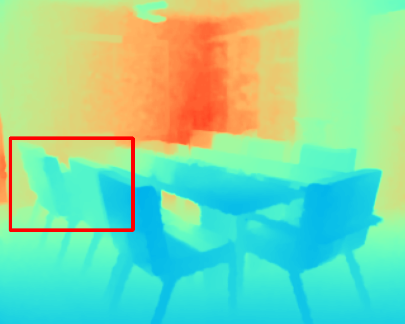
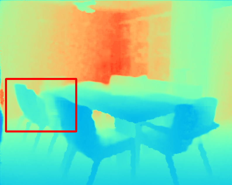
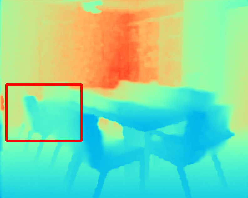
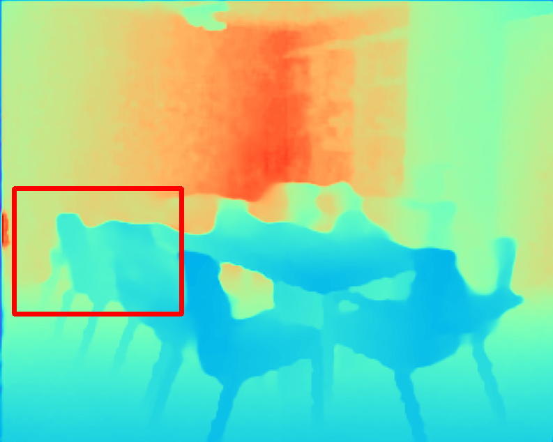
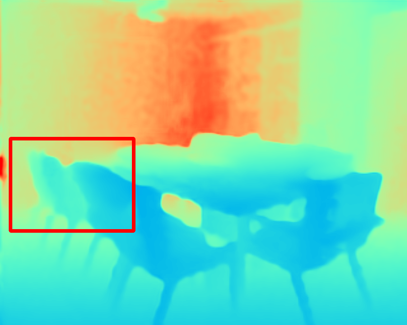
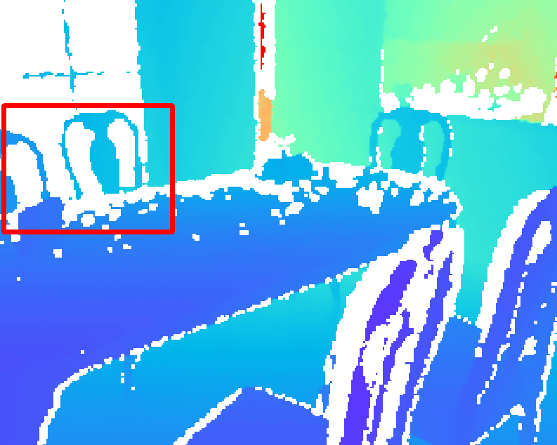
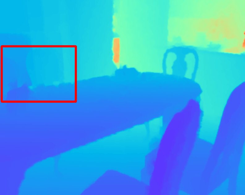
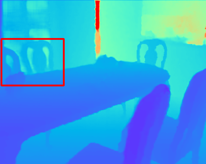
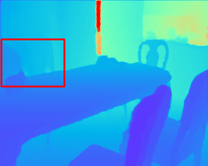
RGB

Sensor

GT

Gansbeke et al.[44]

Li et al.[21]

Huang et al.[16]

ours

Figure 7: Qualitative comparison with Gansbeke et al.[44], Li et al.[21], Huang et al.[16] on NYUv2 [29] test set. All models are trained using our semi-dense sampling strategy. The third and fourth raws present a hard example.

	semi-dense					sparse (500 points)
	RMSE $\downarrow$	rel $\downarrow$	$\delta_{1.25}$ $\uparrow$	$\delta_{1.25^{2}}$ $\uparrow$	$\delta_{1.25^{3}}$ $\uparrow$	RMSE $\downarrow$	rel $\downarrow$	$\delta_{1.25}$ $\uparrow$	$\delta_{1.25^{2}}$ $\uparrow$	$\delta_{1.25^{3}}$ $\uparrow$
Huang et al.[16]	0.271	0.016	98.1	99.1	99.4	–	–	–	–	–
Gansbeke et al.[44]	0.260	0.017	97.9	99.3	99.7	0.344	0.042	96.1	98.5	99.5
Li et al.[21]	0.190	0.018	98.8	99.7	99.9	0.272	0.034	97.3	99.2	99.7
DM-LRN (ours)	0.205	0.014	98.8	99.6	99.9	0.263	0.035	97.5	99.3	99.8

Table 3: NYUv2 TEST. Quantitative comparison of training setups for different models. Semi-dense sampling preserves more accurate information that leads to better results. Although our approach is not intended to be applied to sparse depth sensors, it demonstrates strong results in the sparse training setting in indoor environments. We do not use any densification scheme for target depth reconstruction. Pseudo-sensor data is directly sampled from real sensor data.

ScanNet.

In order to evaluate the generalization capability of our method, we conduct a cross-dataset evaluation. Since the test split was not provided for depth completion on ScanNet, we use 20% of the scenes for testing. For the sake of data diversity, we split all frames into intervals of consecutive 20 frames and take some samples out of each interval. We take the image with the largest variance of Laplacian [34] and the image with the largest file size (which indicates the level of details for a frame). We test the models trained on Matterport3D [4] on this subset that was not seen by the models during the training process. Quantitative results are presented in Table 2, and a qualitative evaluation is shown in Fig. 6. Our method provides sharp depth maps and significantly improves $\delta_{1.05}$, $\delta_{1.10}$, SSIM, and MAE metrics.

RGB
Tang et al. [41]
Li et al. [21]
Gansbeke et al.[44]
Ours

Figure 8: Qualitative comparison with the state-of-art methods on the KITTI test set. Even though our model was designed for a different use case scenario, it is still comparable to the best performing KITTI models in an outdoor environment.

NYUv2.

Since this dataset provides both sensor and reconstruction depth data only for the test subset, we use it to verify our training strategy that does not require ground truth. We first cut off black borders (45, 15, 45, 40 pixels from the top, bottom, left, and right side, respectively) from the original $640\times 480$ RGBD images. Then the images are bilinearly interpolated to $320\times 256$ resolution. These preprocessed RGBD images are used for pseudo sensor data sampling. At test time, the original sensor and ground truth depth data are used. We compare our sampling strategy with the widely used random uniform sampling approach [28, 41]. Qualitative and quantitative results are presented in Fig. 7 and Table 3. Since the original semi-dense depth maps contain more accurate information, our training approach demonstrates significant improvements in all target metrics. The compared performance of models originally designed for sparse inputs is shown in Table 3. Our model demonstrates strong results in this setup as well.

KITTI.

In general, this dataset is out of our scope, since it consists of sparse LiDAR depth measurements. It is a hard case for our model, because the architecture includes a unified encoder for the joint RGBD signal, expecting segments filled with correct depth values. Previous work [21] has demonstrated that it is a suboptimal design for a sparse depth completion model.

Since LiDAR-based outdoor depth completion differs from our use-case scenario, we perform an additional search for the most suitable loss function. As a result, we have chosen the $L_{2}$ loss in the logarithmic domain (see Supplementary material for more details). As the LiDAR points at the top of an image are rare, input images were cropped to $256\times 1216$ for both training and testing, following [41]. A horizontal flip was used as data augmentation.

A quantitative comparison is shown in Table 4. Being designed for semi-dense sensors, our approach demonstrates mid-level performance compared to the KITTI leaderboard. In general, our model produces accurate depth maps, even though there are some errors at the borders of the image.

	RMSE	MAE	iRMSE	iMAE
Cheng et al.[9]	1019	279	2.93	1.15
Gansbeke [44]	773	215	2.19	0.93
Lee et al.[19]	807	254	2.73	1.33
Qiu et al.[35]	758	226	2.56	1.15
Tang et al.[41]	736	218	2.25	0.99
Chen et al.[7]	753	221	2.34	1.14
Li et al.[21]	762	220	2.30	0.98
Ours	984	287	2.67	1.17

Table 4: KITTI TEST. Quantitative comparison with top ranked KITTI models. All metrics are measured in millimeters.

6 Conclusion

In this work, we have proposed a new depth completion method for semi-dense depth sensor maps with auxiliary color images. Our main innovation is a novel decoder architecture that exploits statistical differences between mostly filled and mostly empty regions. It is implemented by an additional decoder modulation branch that takes a mask of missing values as input and adjusts the activation mask distribution in the decoder via SPADE blocks.

In experimental evaluation, our model has shown state-of-the-art results on the Matterport3D dataset with generalization to ScanNet, and even competitive performance on the KITTI dataset with sparse depth measurements. We have also proposed a new training strategy for datasets with raw sensor data and without reconstructed ground truth depth, which allows us to achieve strong results on the NYUv2 dataset.

Appendix A: Loss function ablation study.

Firstly, we investigate how the choice of the loss function affects the performance in different use cases. We search for an appropriate loss function among the popular single-term loss functions that include $L_{1}$ and $L_{2}$ penalties in depth and log-depth domains and their pairwise variations. $L_{1}$ loss family appears to be more efficient for indoor semi-dense depth completion. These functions provide a balance between RMSE and MAE and improve accurate $\delta$-metrics. In other words, they produce clearer edges and boundaries. The pairwise log-$L_{1}$ appears to be the most suitable for Matterport3D. More details can be found in Table 5.

The same search procedure performed on KITTI validation set reveals an advantage of $L_{2}$-family. A good balance was achieved by using these penalties. Even though we choose the log-$L_{2}$ as the main penalty for outdoor LiDAR-oriented depth completion, it can be switched by its pairwise counterpart. A quantitative comparison is shown in Table 6.

	RMSE	MAE	$\delta_{1.25}$	$\delta_{1.25^{2}}$	$\delta_{1.25^{3}}$
$l_{1}$	1.001	0.288	0.888	0.931	0.949
$l_{2}$	0.995	0.311	0.859	0.924	0.948
$\log l_{1}$	1.001	0.289	0.889	0.930	0.948
$\log l_{2}$	1.006	0.318	0.869	0.928	0.949
pairwise $\log l_{1}$	0.961	0.285	0.890	0.933	0.949
pairwise $\log l_{2}$	1.020	0.337	0.859	0.922	0.947

Table 5: Matterport3D TEST. Quantitative comparison of the popular single-term loss functions for depth estimation / completion. RMSE and MAE are measured in meters.

	RMSE	MAE	iRMSE	iMAE
$l_{1}$	1107	279	2.98	1.11
$l_{2}$	1053	304	3.18	1.40
$\log l_{1}$	1108	295	2.89	1.15
$\log l_{2}$	1040	289	2.73	1.15
pairwise $\log l_{1}$	1104	280	2.88	1.08
pairwise $\log l_{2}$	1054	279	2.69	1.07

Table 6: KITTI VALIDATION. Quantitative comparison of the popular single-term loss functions for depth estimation / completion. All metrics are measured in millimeters.

Appendix B: Backbone Depth.

Backbone scalability is an advantage of our approach. In order to investigate the behavior of the model, we carried out additional experiments in which we tried EfficientNets of different sizes. The results are shown in Figure 9. The general trend is predictable: as the size of the network grows, the validation error drops. This is true for the model with and without modulation. The mask modulation consistently gives an improvement in the target metric with the exception ”B3” configuration that demonstrated an unexpected behavior, assumed to be a random outlier. In order to comply with practical applications, we did not try the configurations larger than ”B4”.

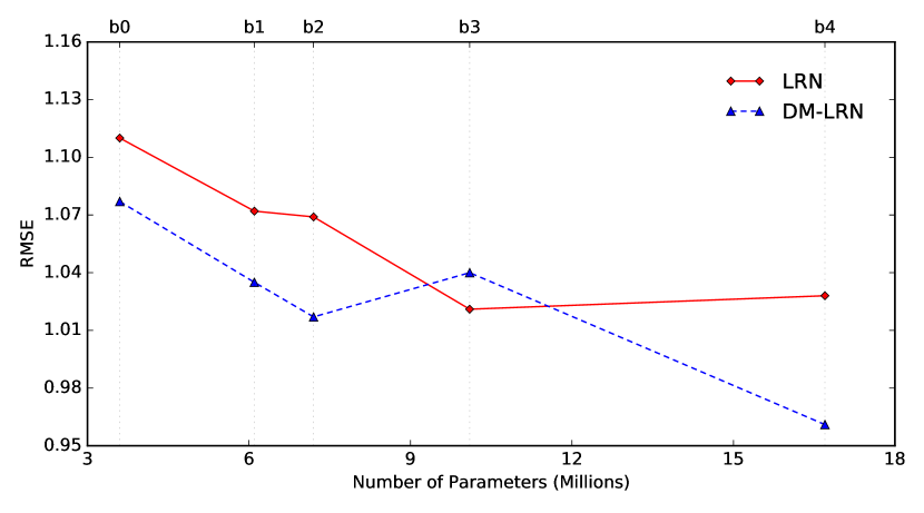
Figure 9: Matterport3D TEST. A dependency of RMSE of the baseline model and the model with the decoder modulation concerning the size of the backbone. LRN is the baseline model with RGBD inputs. DM-LRN is the baseline with the decoder modulation branch.

References

- [1] Ambarella cvflow technology overview. https://www.ambarella.com/technology/technology-overview. Accessed: 2018-10-30.
- [2] R. Achanta, A. Shaji, K. Smith, A. Lucchi, P. Fua, and S. Süsstrunk. Slic superpixels compared to state-of-the-art superpixel methods. IEEE Transactions on Pattern Analysis and Machine Intelligence, 34(11):2274–2282, 2012.
- [3] Vincent Casser, Soeren Pirk, Reza Mahjourian, and Anelia Angelova. Depth prediction without the sensors: Leveraging structure for unsupervised learning from monocular videos. arXiv preprint arXiv:1811.06152, 2018.
- [4] Angel Chang, Angela Dai, Thomas Funkhouser, Maciej Halber, Matthias Niessner, Manolis Savva, Shuran Song, Andy Zeng, and Yinda Zhang. Matterport3d: Learning from rgb-d data in indoor environments. International Conference on 3D Vision (3DV), 2017.
- [5] Liang-Chieh Chen, George Papandreou, Iasonas Kokkinos, Kevin Murphy, and Alan L. Yuille. Deeplab: Semantic image segmentation with deep convolutional nets, atrous convolution, and fully connected crfs. CoRR, abs/1606.00915, 2016.
- [6] Liang-Chieh Chen, George Papandreou, Florian Schroff, and Hartwig Adam. Rethinking atrous convolution for semantic image segmentation. CoRR, abs/1706.05587, 2017.
- [7] Yun Chen, Bin Yang, Ming Liang, and Raquel Urtasun. Learning joint 2d-3d representations for depth completion. In The IEEE International Conference on Computer Vision (ICCV), October 2019.
- [8] Xinjing Cheng, Peng Wang, Chenye Guan, and Ruigang Yang. Cspn++: Learning context and resource aware convolutional spatial propagation networks for depth completion. ArXiv, abs/1911.05377, 2019.
- [9] Xinjing Cheng, Peng Wang, and Ruigang Yang. Depth estimation via affinity learned with convolutional spatial propagation network. In Proceedings of the European Conference on Computer Vision (ECCV), September 2018.
- [10] Angela Dai, Angel X. Chang, Manolis Savva, Maciej Halber, Thomas Funkhouser, and Matthias Nießner. Scannet: Richly-annotated 3d reconstructions of indoor scenes. In Proc. Computer Vision and Pattern Recognition (CVPR), IEEE, 2017.
- [11] David Eigen, Christian Puhrsch, and Rob Fergus. Depth map prediction from a single image using a multi-scale deep network. In Z. Ghahramani, M. Welling, C. Cortes, N. D. Lawrence, and K. Q. Weinberger, editors, Advances in Neural Information Processing Systems 27, pages 2366–2374. Curran Associates, Inc., 2014.
- [12] Pedro F. Felzenszwalb and Daniel P. Huttenlocher. Efficient graph-based image segmentation. Int. J. Comput. Vision, 59(2):167–181, Sept. 2004.
- [13] Huan Fu, Mingming Gong, Chaohui Wang, Kayhan Batmanghelich, and Dacheng Tao. Deep ordinal regression network for monocular depth estimation. In Proceedings of the IEEE Conference on Computer Vision and Pattern Recognition, pages 2002–2011, 2018.
- [14] C. Godard, O. M. Aodha, and G. J. Brostow. Unsupervised monocular depth estimation with left-right consistency. In 2017 IEEE Conference on Computer Vision and Pattern Recognition (CVPR), pages 6602–6611, 2017.
- [15] S. Hawe, M. Kleinsteuber, and K. Diepold. Dense disparity maps from sparse disparity measurements. In 2011 International Conference on Computer Vision, pages 2126–2133, 2011.
- [16] Yu-Kai Huang, Tsung-Han Wu, Yueh-Cheng Liu, and Winston H. Hsu. Indoor depth completion with boundary consistency and self-attention. 2019 IEEE/CVF International Conference on Computer Vision Workshop (ICCVW), Oct 2019.
- [17] Diederik P. Kingma and Jimmy Ba. Adam: A method for stochastic optimization. In Yoshua Bengio and Yann LeCun, editors, 3rd International Conference on Learning Representations, ICLR 2015, San Diego, CA, USA, May 7-9, 2015, Conference Track Proceedings, 2015.
- [18] Katrin Lasinger, René Ranftl, Konrad Schindler, and Vladlen Koltun. Towards robust monocular depth estimation: Mixing datasets for zero-shot cross-dataset transfer. CoRR, abs/1907.01341, 2019.
- [19] S. Lee, J. Lee, D. Kim, and J. Kim. Deep architecture with cross guidance between single image and sparse lidar data for depth completion. IEEE Access, 8:79801–79810, 2020.
- [20] Anat Levin, Dani Lischinski, and Yair Weiss. Colorization using optimization. ACM Trans. Graph., 23(3):689–694, Aug. 2004.
- [21] Ang Li, Zejian Yuan, Yonggen Ling, Wanchao Chi, Chong Zhang, et al. A multi-scale guided cascade hourglass network for depth completion. In The IEEE Winter Conference on Applications of Computer Vision, pages 32–40, 2020.
- [22] Ang Li, Zejian Yuan, Yonggen Ling, Wanchao Chi, shenghao zhang, and Chong Zhang. A multi-scale guided cascade hourglass network for depth completion. In The IEEE Winter Conference on Applications of Computer Vision (WACV), March 2020.
- [23] Zhengqi Li and Noah Snavely. Megadepth: Learning single-view depth prediction from internet photos. CoRR, abs/1804.00607, 2018.
- [24] Zhengfa Liang, Yiliu Feng, YGHLW Chen, and LQLZJ Zhang. Learning for disparity estimation through feature constancy. In Proceedings of the IEEE Conference on Computer Vision and Pattern Recognition, pages 2811–2820, 2018.
- [25] Guosheng Lin, Anton Milan, Chunhua Shen, and Ian Reid. Refinenet: Multi-path refinement networks for high-resolution semantic segmentation. pages 5168–5177, 07 2017.
- [26] L. Liu, S. H. Chan, and T. Q. Nguyen. Depth reconstruction from sparse samples: Representation, algorithm, and sampling. IEEE Transactions on Image Processing, 24(6):1983–1996, 2015.
- [27] Wenjie Luo, Alexander G Schwing, and Raquel Urtasun. Efficient deep learning for stereo matching. In Proceedings of the IEEE Conference on Computer Vision and Pattern Recognition, pages 5695–5703, 2016.
- [28] Fangchang Ma and Sertac Karaman. Sparse-to-dense: Depth prediction from sparse depth samples and a single image. 2018.
- [29] Pushmeet Kohli Nathan Silberman, Derek Hoiem and Rob Fergus. Indoor segmentation and support inference from rgbd images. In ECCV, 2012.
- [30] Vladimir Nekrasov, Thanuja Dharmasiri, Andrew Spek, Tom Drummond, Chunhua Shen, and Ian Reid. Real-time joint semantic segmentation and depth estimation using asymmetric annotations. pages 7101–7107, 05 2019.
- [31] Vladimir Nekrasov, Chunhua Shen, and Ian D. Reid. Light-weight refinenet for real-time semantic segmentation. In British Machine Vision Conference 2018, BMVC 2018, Northumbria University, Newcastle, UK, September 3-6, 2018, page 125. BMVA Press, 2018.
- [32] T. Park, M. Liu, T. Wang, and J. Zhu. Semantic image synthesis with spatially-adaptive normalization. In 2019 IEEE/CVF Conference on Computer Vision and Pattern Recognition (CVPR), pages 2332–2341, 2019.
- [33] Adam Paszke, Sam Gross, Francisco Massa, Adam Lerer, James Bradbury, Gregory Chanan, Trevor Killeen, Zeming Lin, Natalia Gimelshein, Luca Antiga, Alban Desmaison, Andreas Kopf, Edward Yang, Zachary DeVito, Martin Raison, Alykhan Tejani, Sasank Chilamkurthy, Benoit Steiner, Lu Fang, Junjie Bai, and Soumith Chintala. Pytorch: An imperative style, high-performance deep learning library. In H. Wallach, H. Larochelle, A. Beygelzimer, F. d Alché-Buc, E. Fox, and R. Garnett, editors, Advances in Neural Information Processing Systems 32, pages 8024–8035. Curran Associates, Inc., 2019.
- [34] Jose Luis Pech Pacheco, Gabriel Cristobal, J. Chamorro-Martinez, and J. Fernandez-Valdivia. Diatom autofocusing in brightfield microscopy: A comparative study. volume 3, pages 314–317 vol.3, 02 2000.
- [35] Jiaxiong Qiu, Zhaopeng Cui, Yinda Zhang, Xingdi Zhang, Shuaicheng Liu, Bing Zeng, and Marc Pollefeys. Deeplidar: Deep surface normal guided depth prediction for outdoor scene from sparse lidar data and single color image. In The IEEE Conference on Computer Vision and Pattern Recognition (CVPR), June 2019.
- [36] Haoyu Ren, Aman Raj, Mostafa El-Khamy, and Jungwon Lee. Suw-learn: Joint supervised, unsupervised, weakly supervised deep learning for monocular depth estimation. In Proceedings of the IEEE/CVF Conference on Computer Vision and Pattern Recognition (CVPR) Workshops, June 2020.
- [37] Mikhail Romanov, Nikolay Patatkin, Anna Vorontsova, and Anton Konushin. Towards general purpose and geometry preserving single-view depth estimation, 2020.
- [38] O. Ronneberger, P.Fischer, and T. Brox. U-net: Convolutional networks for biomedical image segmentation. In Medical Image Computing and Computer-Assisted Intervention (MICCAI), volume 9351 of LNCS, pages 234–241. Springer, 2015. (available on arXiv:1505.04597 [cs.CV]).
- [39] S. S. Shivakumar, T. Nguyen, I. D. Miller, S. W. Chen, V. Kumar, and C. J. Taylor. Dfusenet: Deep fusion of rgb and sparse depth information for image guided dense depth completion. In 2019 IEEE Intelligent Transportation Systems Conference (ITSC), pages 13–20, 2019.
- [40] Mingxing Tan and Quoc Le. EfficientNet: Rethinking model scaling for convolutional neural networks. In Kamalika Chaudhuri and Ruslan Salakhutdinov, editors, Proceedings of the 36th International Conference on Machine Learning, volume 97 of Proceedings of Machine Learning Research, pages 6105–6114, Long Beach, California, USA, 09–15 Jun 2019. PMLR.
- [41] Jie Tang, Fei-Peng Tian, Wei Feng, Jian Li, and Ping Tan. Learning guided convolutional network for depth completion. ArXiv, abs/1908.01238, 2019.
- [42] Jonas Uhrig, Nick Schneider, Lukas Schneider, Uwe Franke, Thomas Brox, and Andreas Geiger. Sparsity invariant cnns. 2017 International Conference on 3D Vision (3DV), pages 11–20, 2017.
- [43] W. Van Gansbeke, D. Neven, B. De Brabandere, and L. Van Gool. Sparse and noisy lidar completion with rgb guidance and uncertainty. In 2019 16th International Conference on Machine Vision Applications (MVA), pages 1–6, 2019.
- [44] Wouter Van Gansbeke, Davy Neven, Bert De Brabandere, and Luc Van Gool. Sparse and noisy lidar completion with rgb guidance and uncertainty. In 2019 16th International Conference on Machine Vision Applications (MVA), pages 1–6. IEEE, 2019.
- [45] Andrea Vedaldi and Stefano Soatto. Quick shift and kernel methods for mode seeking. In David A. Forsyth, Philip H. S. Torr, and Andrew Zisserman, editors, ECCV (4), volume 5305 of Lecture Notes in Computer Science, pages 705–718. Springer, 2008.
- [46] Wofk, Diana and Ma, Fangchang and Yang, Tien-Ju and Karaman, Sertac and Sze, Vivienne. FastDepth: Fast Monocular Depth Estimation on Embedded Systems. In IEEE International Conference on Robotics and Automation (ICRA), 2019.
- [47] Yan Xu, Xinge Zhu, Jianping Shi, Guofeng Zhang, Hujun Bao, and Hongsheng Li. Depth completion from sparse lidar data with depth-normal constraints. In The IEEE International Conference on Computer Vision (ICCV), October 2019.
- [48] Yanchao Yang, Alex Wong, and Stefano Soatto. Dense depth posterior (ddp) from single image and sparse range. In The IEEE Conference on Computer Vision and Pattern Recognition (CVPR), June 2019.
- [49] Amir R. Zamir, Alexander Sax, William B. Shen, Leonidas J. Guibas, Jitendra Malik, and Silvio Savarese. Taskonomy: Disentangling task transfer learning. In IEEE Conference on Computer Vision and Pattern Recognition (CVPR). IEEE, 2018.
- [50] Yinda Zhang and Thomas A. Funkhouser. Deep depth completion of a single RGB-D image. CoRR, abs/1803.09326, 2018.
- [51] Hengshuang Zhao, Jianping Shi, Xiaojuan Qi, Xiaogang Wang, and Jiaya Jia. Pyramid scene parsing network. CoRR, abs/1612.01105, 2016.