DDD20 End-to-End Event Camera Driving Dataset: Fusing Frames and Events with Deep Learning for Improved Steering Prediction

Abstract

Neuromorphic event cameras are useful for dynamic vision problems under difficult lighting conditions. To enable studies of using event cameras in automobile driving applications, this paper reports a new end-to-end driving dataset called DDD20. The dataset was captured with a DAVIS camera that concurrently streams both dynamic vision sensor (DVS) brightness change events and active pixel sensor (APS) intensity frames. DDD20 is the longest event camera end-to-end driving dataset to date with 51h of DAVIS event+frame camera and vehicle human control data collected from 4000 km of highway and urban driving under a variety of lighting conditions. Using DDD20, we report the first study of fusing brightness change events and intensity frame data using a deep learning approach to predict the instantaneous human steering wheel angle. Over all day and night conditions, the explained variance for human steering prediction from a Resnet-32 is significantly better from the fused DVS+APS frames (0.88) than using either DVS (0.67) or APS (0.77) data alone.

I INTRODUCTION

Recent advances in autonomous driving [1, 2, 3, 4, 5] have been fueled by modern deep learning methods, whereby driving controllers are typically trained on extensive datasets of real-world recordings and simulated environments [6, 7, 8, 9, 10]. The availability of these datasets together with advances in deep learning has enabled improvements in computer vision technologies that are essential to the success of autonomous driving, such as semantic segmentation [11], object detection, tracking [12], and motion estimation [13].

Self-driving vehicles must operate under a wide range of lighting conditions, and thus it is crucial that employed vision sensors offer high dynamic range and high sensitivity, enabling short exposure times to minimize motion blur. Event cameras such as Dynamic Vision Sensors (DVS) [14] can offer advantages under conditions that are difficult for conventional cameras. In contrast to regular-sampled, frame-based cameras, event cameras produce a stream of asynchronous timestamped address events that are triggered by local brightness (log intensity) changes at individual pixels. Fig. 1(a) shows the principle of the DVS pixel response. The DVS responds the same way to equal contrast variations (typically caused by scene reflectance changes) independent of absolute intensity. The local instantaneous gain control enables a broader dynamic range than conventional cameras (120dB vs. 60dB) for handling uncontrolled lighting conditions. These events are transmitted off-chip with submillisecond latency. Each event includes the pixel coordinates, the sign of the brightness change, and the microsecond timestamp. The asynchronous nature of DVS events reduces the latency and bandwidth requirements of the system, enabling robots with millisecond response times at low average CPU load. Automotive cameras require special pixel architectures to minimize frame-to-frame aliasing of pulse-width-modulated LED light sources like car taillights and traffic sign light sources. The high temporal resolution of the DVS events enables accurate CNN-based [15] and sub-ms hardware-based [16] optical flow estimation and flashing light source detection and tracking [17].

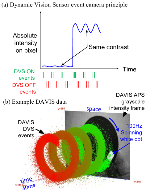
Figure 1: (a) Concept of DVS event camera pixel response; (b) DAVIS frame + event camera data from 100 Hz spinning dot.

Fig. 1(b) shows output from a next generation event camera called Dynamic and Active-Pixel Vision Sensor (DAVIS) [18]. A DAVIS concurrently outputs both DVS events (the spiral cloud of points in Fig. 1(b)), and standard global-shutter active pixel sensor (APS) intensity frames (background image in Fig. 1(b)). The DVS and APS pixel circuits that share the same photodiode. The combination of sampled analog gray values from the APS stream and the asynchronous, high dynamic range brightness change events from the DVS could make the DAVIS well-suited to driving applications: When the APS stream is over- or under-exposed, or the features are blurred or aliased, the DVS events can provide the missing information.

I-A Related work

[19] showed that fused DAVIS frame+event data could drive a CNN to steer a predator robot to follow a prey robot. It inspired us to investigate benefits that the DAVIS camera could provide for autonomous driving. To avoid expensive data labeling as in [19], we followed the pioneering end-to-end (E2E) studies dating back to ALVINN [20, 21], and more recently comma.ai and NVIDIA [1, 9], where the network directly predicts the human’s instantaneous steering wheel angle based on the appearance of the road.

Our first dataset called DDD17, containing 12h of E2E labeled driving data [22], was used by [23] to compare the human steering with predictions using APS frames, APS frame differences, and DVS frames. They showed that DVS frames gave better steering prediction than APS frames (in contrast to our findings in Sec. III-B), and better prediction than APS frame differences, however, they did not evaluate the benefit of fusing DVS and APS data. [23] also found that ResNet CNN architectures are well suited to the steering prediction problem, and that a DVS ‘frame’ duration of 50ms produced the best predictions.

DDD17 was limited in road types, weather and daylight conditions. Since then, MVSEC [24], DET [25], Event Camera Driving Sequences [26], and GET1 [27] datasets have been released. These datasets contain useful driving data with various label types, but none of them are E2E labeled with human driving.

I-B DDD20

To allow more extensive E2E studies, we expanded the 12 h DDD17 with an additional 39 h of data, giving the new DDD20 dataset. It has a total of 1.3 TB of data with 51 h of recordings collected from a $346\times 260$-pixel DAVIS346 camera, along with car parameters such as steering wheel angle. DDD20 has recordings of rural highway driving under difficult sunlight glare conditions, day and night driving in urban Los Angeles and San Diego, and multiple repeats of the same sections of mountain highway driving (along the Colorado Lizard Head Pass highway and California Angeles Crest Highway) during daylight, evening, and night. Section II contains details of the dataset.

Fig. 2 shows examples of how the APS and DVS streams from DDD20 complement each other. For the frame pair outlined in red, the stopped car is invisible in the DVS frame, but cars in other lanes pop out in the DVS frame because of their motion. For some scenes (e.g. left middle), the road edge is not visible in the DVS frame because the car is driving straight along the road. In others (e.g. top middle), the upcoming curve is visible in the DVS frame because the car is approaching the curve. In many scenes the APS frame is underexposed, overexposed, or motion blurred, but in the DVS frame, the object is still visible because of its superior dynamic range and quicker response. A properly trained network should take advantage of this complementary APS and DVS information. We demonstrate this using a network for steering prediction in Sec. III.

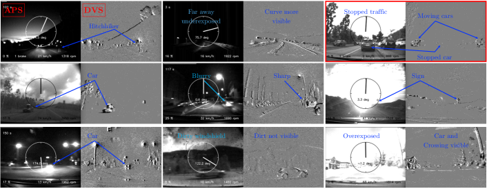
Figure 2: DDD20 sample data. Each pair of frames show APS (left) and DVS (right) data. DVS signed event histogram frame durations are 25 ms. APS frame exposure duration varies with illumination from 50 us to about 200 ms.

DDD20 includes E2E vehicle control and diagnostics data to allow studies of the effectiveness of the DAVIS camera compared to standard grayscale image sensors. It does not contain LIDAR, radar, and other sensors necessary for a complete ADAS solution.

The main contributions of this paper are

1. The DDD20 dataset, with the methods and software used for the dataset collection. (Sec. II).

2. The use of DDD20 for the first study of fusing of APS and DVS data for steering prediction (Sec. III). In contrast to [23], we find that APS frames produce better steering prediction results than DVS frames alone. In addition, we show that fusing APS and DVS data improves the predictions by a significant margin over either modality by itself.

II METHODS

The ‘DAVIS Driving Dataset 2020’ (DDD20) dataset will be released at http://sensors.ini.uzh.ch/databases.html . This section describes the DAVIS camera and how we collected the dataset.

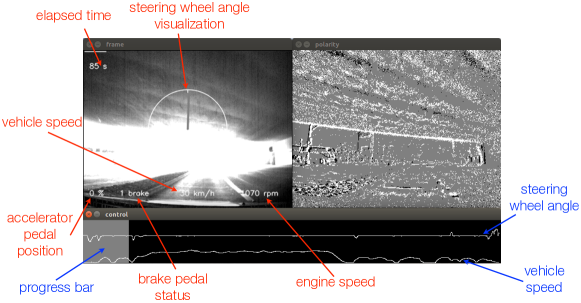
Figure 3: Example DDD20 recording visualized by the viewer application. The top panels display APS (top-left) and DVS (top-right) frames. The bottom panel controls and shows the status of the recording. Various vehicle data fields are presented as well. In this example, the APS frame suffers from over and underexposure, while the DVS frame still exposes these details.

II-A DAVIS camera setup

Camera input was captured from our DAVIS346B [28]. It produces both DVS events and APS frames that are concurrently captured from the same optics. Each pixel uses the same photodiode for producing DVS and APS outputs simultaneously. The DAVIS346B with 346$\times$260 pixels is similar to the DAVIS240C [18], but has 2.1$\times$ more pixels and includes on-chip column parallel analog-to-digital converters (ADCs) for an APS frame rate of up to 50 Hz. The DAVIS346B also has buried photodiodes with microlenses and anti-reflection coating that increases the quantum efficiency by a factor of about 4, and reduces the photodiode dark current. In the original DDD17 recordings, we used a 6 mm lens providing a 56^∘ horizontal field of view (FOV). For the DDD20 recordings, we increased the FOV to 71^∘ to cover more road features during turns by using a Kowa 4.5 mm.

The APS frame rate depends on the auto-exposure duration. In later recordings, this duration was set by an auto exposure algorithm that optimized the exposure time for the road surface in the lower third of the image. Thus the frame rate (and exposure duration) varies between 8 fps and 50 fps. In some recordings, the frame rate was also limited to reduce file size. The frames were captured using the DAVIS global shutter mode to minimize motion artifacts.

The camera was mounted using a glass suction tripod fixed behind the windshield, just below the rear mirror, and aligned to point to the center of the hood. The original DDD17 Ford Mondeo dataset (see Sec. II-B) used a single mounting point. For the Ford Focus recordings, the sensor was mounted each day and adjusted to bring the edge of the hood to the bottom of the frame, centered on the road; thus recordings have slightly different viewpoints. The USB3.0 camera was connected to a laptop computer and was read out using cAER, which streamed it by local UDP to the recording framework described in Sec. II-C.

II-B Vehicle control and diagnostic data collection

Data was acquired using a 2015 Ford Mondeo MK3 European Model for Swiss/German recordings and a 2016 Ford Focus for USA recordings. A $130 OpenXC Ford Reference vehicle interface was connected to the passenger compartment OBDII port, and read out control and diagnostic data from the car’s CAN bus. The vehicle interface was connected to the laptop USB port. The vehicle interface was read out using the OpenXC python library, and passed to the custom recording software described in Sec. II-C. Data including the examples in Table I was sampled at about 10 Hz.

II-C Recording and viewing software

The Python software framework ddd20-utils records, views and exports recordings (Fig. 3). Since the APS frames and DVS data are microsecond time-stamped on the camera using its clock unlike the data provided by the vehicle interface, both data streams were augmented with the millisecond system time of the recording computer so that the car and camera streams can be synchronized. When possible, the computer time was synchronized to a standard time server before recordings. The streams were processed by separate threads. Although the camera and car interface each have their own precision clocks, it was most straightforward to use the computer time to synchronize the two streams, because the vehicle sample rate is only about 10 Hz. The data is stored in HDF5 containers.

TABLE I: Subset of vehicle control and diagnostic data

ID	Data Field	Unit	Range
1.	accelerator pedal position	percent	0–100%
2.	brake pedal status	binary	pressed/released
3.	engine speed	rpm
4.	headlamp status	binary	ON/OFF
5.	latitude	degrees
6.	longitude	degrees
7.	odometer	km or miles
8.	steering wheel angle	degrees	up to $\pm$720∘
9.	transmission gear position	gear no.	1 to 6
10.	vehicle_speed	km/h	0-160
11.	windshield wiper status	binary	ON/OFF

II-D Recorded DDD20 data

The 51 h of usable data were recorded under various weather, driving, road, and lighting conditions over about 60 days of intermittent recording. Recordings were started and stopped manually. They have durations between a few minutes and an hour, with a median length of about 700 s. The 40 recordings of the original DDD17 were supplemented by an additional 175 recordings in DDD20. Steering angles on straight roads were dominated by small deviations of $\pm 10{{}^{\circ}}$. The car speed was uniformly distributed over the range of 0–130 km/h.

III EXPERIMENTS

This section reports experiments using DDD20 to address the question of whether fusing APS and DVS together provides better steering prediction than either single modality.

III-A Experiment configurations

III-A1 Data selection

We selected 30 recordings from DDD20 that covered a range of road types and lighting conditions, with 15 night and 15 day recordings (recordings used are reported on DDD20 website). We manually pruned the ends where the car was pulling onto or off the road. For each recording, we chose the first 70% of the data as a part of the training data and the last 30% as a part of the test data. Then, we prepared three datasets: Night, Day, and All. These datasets let us study the network’s predication accuracy with different choices of sensor input (DVS+APS, DVS-only, and APS-only) under day versus night lighting conditions.

III-A2 Preprocessing inputs for training

[23] showed that a 50 ms DVS frame duration provided the optimum for DVS steering prediction using our original DDD17 dataset [22]. Hence we used DVS frames of 2D histograms of signed ON/OFF DVS event counts accumulated for 50 ms to approximately match the average APS frame rate. With this integration time, motion blurring was acceptable for normal passenger car dynamics. The DVS histogram was then clipped at three times its standard deviation. For APS-only prediction, we used the APS frames at their native sample rate. When the APS frame rate was lower than 20Hz, we duplicated the APS frames. The resulting DVS frames and the corresponding APS grayscale frames were both rescaled to the range $[0,1]$ following the procedure established in [19].

Speeds below 15 km/h were eliminated because they generally signal when the car was exiting a parking space or turning a corner at an intersection. When the car is stopped, the driver sometimes plays with the wheel for a while, leaving it then stopped at a random angle. This simple exclusion works well for our current steering prediction because each prediction is based on the instantaneous DVS+APS frame, and it is not possible to know the intention of the driver such as when they are backing out of a space or deciding to make a turn at a corner.

The distribution of the steering angles is unbalanced because straight driving dominates the recordings. Therefore, we randomly pruned 70% of those frames that have steering angles between $\pm 5^{\circ}$. We also filtered out frames where the steering angles are larger than three times the standard deviation of all steering because these generally represent outliers such as pulling off the road. Pruning leaves about 50% of the frames from the original training dataset. In the test dataset, we only filtered out the extra large steering angle and low-speed frame outliers.

To reduce computation, the original APS and DVS frames were subsampled from $346\times 260$ to $172\times 128$ pixels where we could still clearly see the road ahead. We aligned the camera and car inputs using the system clock timestamp.

III-A3 Baseline network

Based on [23], we chose the 32-layer Residual Network (ResNet-32) as the baseline network to study the steering angle prediction. The configuration for the convolution layers is identical to the one in [29]. The output layer is a linear layer that has one output for predicting the steering angle. Fig. 5 shows the architecture. In the cases of DVS-only and APS-only, the network is trained with a one-channel input. The network has 470k parameters and has about 400M connections.

Figure 4: Experiment results for rec1501288723.hdf5. Top figures show the 700th APS and DVS frames. The black vertical line in the plot also indicate the 700th frame. All networks can successfully predict the steering wheel angle but the DVS+APS one is most accurate. Shadings show $1\sigma$ standard deviation over 5 training/test runs.

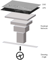
Figure 5: Illustration of the steering prediction network in this paper.

III-A4 Training details

The weight parameters were initialized following [29] by sampling from a Gaussian distribution $\mathcal{N}(0,2/\sqrt{n_{\textrm{in}}})$, where $n_{\textrm{in}}$ is the number of input neurons. Our dataset was large enough so that we did not need to pretrain on a different dataset, as in [23]. Biases were initialized to zero. Models were trained using a weight decay of $10^{-4}$ using the Adam optimizer [30] with an initial learning rate of $10^{-3}$. The networks were trained for 200 epochs, using minibatches of 128 samples and using a Mean Squared Error (MSE) loss. Training time for one run on the prepared dataset using one NVIDIA K80 GPU took about 24 hours.

III-B Prediction of steering wheel angle

Fig. 4 shows an example of the steering angle prediction. The top row shows example APS and DVS images. The bottom plot compares the ground truth steering wheel angle with the APS, DVS, and DVS+APS prediction results. While the three prediction curves appear similar, the prediction made by DVS+APS (in brown) is slightly more accurate. The dataset web site includes videos comparing predictions from DVS, APS, and DVS+APS for all paper dataset recordings.

Table II summarizes the RMS steering wheel angle prediction error (RMSE) and standard deviation achieved for each dataset using the combination of DVS and APS input channels. The standard deviation was computed over 5 repeats of each experiment, each time using different random seeds for weight initialization.

The explained variance (EVA) also measures prediction accuracy. The EVA of steering angle $\Omega$, is defined by ${\rm EVA}=1-{\text{Var}(\vec{\Omega}_{\rm pred}-\vec{\Omega}_{\rm gt})/\text{Var}(\vec{\Omega}_{\rm gt})}$, where $\vec{\Omega}_{\rm pred}$ and $\vec{\Omega}_{\rm gt}$ are the predicted and ground truth angles for all samples in the test set. EVA is dimensionless and ranges from approximately 0 to 1. The closer to 1, the better the prediction.

Both RMSE and EVA are useful for understanding the results. For example, the EVA for straight driving is usually quite low, indicating that the detailed timing of the small steering corrections when driving straight are not very well predicted. Since the RMSE is also small in this case, it means that prediction poorly reflects the details of steering but still well-predicts small angles. (During straight driving, humans only occasionally correct off-center lane positions, and it is impossible to predict—especially from single frames—when these corrections occur.)

TABLE II: Steering wheel prediction error using RMSE and EVA. The colored bar shows the results of three datasets.

Dataset	RMSE (∘) (lower is better)
	DVS+APS	DVS	APS
Night	$\mathbf{2.79\pm 0.15}$	$4.17\pm 0.16$	$3.49\pm 0.06$
Day	$\mathbf{5.48\pm 0.44}$	$7.77\pm 0.68$	$7.30\pm 0.38$
All	$\mathbf{4.13\pm 0.24}$	$6.53\pm 0.34$	$5.60\pm 0.25$
	EVA (higher is better)
	DVS+APS	DVS	APS
Night	$\mathbf{0.931\pm 0.008}$	$0.851\pm 0.011$	$0.893\pm 0.005$
Day	$\mathbf{0.760\pm 0.022}$	$0.487\pm 0.091$	$0.537\pm 0.049$
All	$\mathbf{0.881\pm 0.009}$	$0.668\pm 0.032$	$0.765\pm 0.018$

The bold quantities in Table II highlight the best steering prediction results for each dataset. The EVAs are compared graphically below the table. It is clear that using DVS+APS results in the best steering prediction. A trivial baseline prediction error is obtained by fixing the prediction to to $0^{\circ}$ (always driving straight). This null prediction yields RMSE of $11^{\circ}$ and EVA of $0$, which also corresponds to the standard deviation of steering angle.

Even the worst RMSE of 7.8^∘ and EVA of 0.49 obtained using only DVS in daylight conditions are better than the null prediction. Over all three datasets, the DVS+APS models achieve the best average steering angle prediction (EVA 0.88), which are slightly better than the best results obtained by [23] (0.83). (Additionally, [23] used a larger ResNet-50, and tested on interleaved time segments from each recording; i.e. the training used 40 s sections of road immediately surrounding 20 s testing sections). The EVA for DVS+APS is significantly better than for either DVS or APS alone. It seems that the moving features exposed by the DVS improve the steering predictions. Overall, these results indicate that the combined DVS and APS inputs help the network make more accurate predictions.

Our overall EVA of $0.67\pm.03$ for DVS-only prediction are consistent with [23], who obtained overall EVA of 0.72. But in sharp contrast, we found that APS frames consistently produced better EVA of $0.77\pm.02$, while [23] reported an overall APS-only EVA of only 0.40. A higher EVA from APS frames might be expected, because the finer gray scale would generally allow seeing road versus non-road more clearly.

The nighttime steering predictions (EVA 0.93) are clearly better than daytime predictions (EVA 0.76). We believe it is because the headlights do well to light the roadway to allow perception of the upcoming curves. For daytime conditions, the fused APS+DVS provides a large improvement of the EVA; it is more than 40% higher with fused input than with either of the single inputs. We believe that it is from from the DVS better handling glare and overexposure.

IV CONCLUSIONS

DDD20 is the first open E2E driving dataset with over 50 h of recordings from a DAVIS event camera mounted on a vehicle driven over 4000 km. The dataset increases the size of the original DDD17 dataset by a factor of about 4$\times$. In terms of both driving duration and distance, DDD20 is comparable to the 72h NVIDIA dataset used in [1] and the 10000 km Baidu dataset [10]. (The BDD100k dataset [31] is far larger (1100h), but it is not E2E.)

We show the first results on end-to-end steering prediction with the fused APS and DVS sensor input. Our results show that fused DVS and APS information best explains the steering variance under all driving conditions. Without temporal context, the DVS is blind to non-moving features that are common in driving, but provides valuable information to improve APS prediction.

Future work could exploit the fine timing of the DVS events, for example, to preprocess the input for optical flow, to compute inference on DVS interframes, and to incorporate temporal context into the predictions. This temporal context could better enable prediction of throttle and braking decisions that are difficult using single frames.

References

- [1] M. Bojarski, D. D. Testa, D. Dworakowski, B. Firner, B. Flepp, P. Goyal, L. D. Jackel, M. Monfort, U. Muller, J. Zhang, X. Zhang, J. Zhao, and K. Zieba, “End to end learning for self-driving cars,” CoRR, vol. abs/1604.07316, 2016.
- [2] C. Chen, A. Seff, A. Kornhauser, and J. Xiao, “DeepDriving: Learning affordance for direct perception in autonomous driving,” in Proceedings of the 2015 IEEE International Conference on Computer Vision (ICCV), ser. ICCV ’15. Washington, DC, USA: IEEE Computer Society, 2015, pp. 2722–2730.
- [3] S. Sharifzadeh, I. Chiotellis, R. Triebel, and D. Cremers, “Learning to drive using inverse reinforcement learning and deep Q-networks,” in NIPS workshop on Deep Learning for Action and Interaction, 2016.
- [4] H. Xu, Y. Gao, F. Yu, and T. Darrell, “End-to-end learning of driving models from large-scale video datasets,” in The IEEE Conference on Computer Vision and Pattern Recognition (CVPR), 2017.
- [5] S. Grigorescu, B. Trasnea, T. Cocias, and G. Macesanu, “A survey of deep learning techniques for autonomous driving,” Journal of Field Robotics, 2019.
- [6] M. Cordts, M. Omran, S. Ramos, T. Rehfeld, M. Enzweiler, R. Benenson, U. Franke, S. Roth, and B. Schiele, “The Cityscapes dataset for semantic urban scene understanding,” in The IEEE Conference on Computer Vision and Pattern Recognition (CVPR), 2016.
- [7] A. Geiger, “Are we ready for autonomous driving? The KITTI vision benchmark suite,” in IEEE Conference on Computer Vision and Pattern Recognition (CVPR). Washington, DC, USA: IEEE Computer Society, 2012, pp. 3354–3361.
- [8] W. Maddern, G. Pascoe, C. Linegar, and P. Newman, “1 Year, 1000km: The Oxford RobotCar Dataset,” The International Journal of Robotics Research (IJRR), vol. 36, no. 1, pp. 3–15, 2017.
- [9] E. Santana and G. Hotz, “Learning a driving simulator,” CoRR, vol. abs/1608.01230, 2016.
- [10] H. Yu, S. Yang, W. Gu, and S. Zhang, “Baidu driving dataset and end-to-end reactive control model,” in IEEE Intelligent Vehicles Symposium, IV 2017, Los Angeles, CA, USA, 2017, pp. 341–346.
- [11] H. Zhao, J. Shi, X. Qi, X. Wang, and J. Jia, “Pyramid scene parsing network,” in IEEE Conference on Computer Vision and Pattern Recognition (CVPR), 2017.
- [12] S. Ren, K. He, R. Girshick, and J. Sun, “Faster R-CNN: Towards real-time object detection with region proposal networks,” in Advances in Neural Information Processing Systems 28, C. Cortes, N. D. Lawrence, D. D. Lee, M. Sugiyama, and R. Garnett, Eds. Curran Associates, Inc., 2015, pp. 91–99.
- [13] A. Kendall, M. Grimes, and R. Cipolla, “PoseNet: A convolutional network for real-time 6-DOF camera relocalization,” in Proceedings of the International Conference on Computer Vision (ICCV), 2015.
- [14] P. Lichtsteiner, C. Posch, and T. Delbruck, “A 128x128 120 dB 15 s latency asynchronous temporal contrast vision sensor,” IEEE Journal of Solid-State Circuits, vol. 43, no. 2, pp. 566–576, Feb 2008.
- [15] A. Z. Zhu, L. Yuan, K. Chaney, and K. Daniilidis, “EV-FlowNet: Self-supervised optical flow estimation for event-based cameras,” CoRR, vol. abs/1802.06898, 2018.
- [16] M. Liu and T. Delbruck, “Adaptive time-slice block-matching optical flow algorithm for Dynamic Vision Sensors,” in Proceedings of British Machine Vision Conference (BMVC 2018), Newcastle upon Tyne, UK, Sept. 2018.
- [17] G. R. Müller and J. Conradt, “A miniature low-power sensor system for real time 2D visual tracking of LED markers,” in 2011 IEEE International Conference on Robotics and Biomimetics, Dec. 2011, pp. 2429–2434.
- [18] C. Brandli, R. Berner, M. Yang, S.-C. Liu, and T. Delbruck, “A 240180 130 dB 3 s latency global shutter spatiotemporal vision sensor,” IEEE Journal of Solid-State Circuits, vol. 49, no. 10, pp. 2333–2341, 2014.
- [19] D. P. Moeys, F. Corradi, E. Kerr, P. Vance, G. Das, D. Neil, D. Kerr, and T. Delbrück, “Steering a predator robot using a mixed frame/event-driven convolutional neural network,” in 2016 Second International Conference on Event-based Control, Communication, and Signal Processing (EBCCSP), Jun 2016, pp. 1–8.
- [20] D. A. Pomerleau, “ALVINN: An autonomous land vehicle in a neural network,” in Advances in Neural Information Processing Systems 1, D. S. Touretzky, Ed. Morgan-Kaufmann, 1989, pp. 305–313.
- [21] ——, Neural network perception for mobile robot guidance. Springer Science & Business Media, 2012, vol. 239.
- [22] J. Binas, D. Neil, S.-C. Liu, and T. Delbruck, “DDD17: End-to-end DAVIS driving dataset,” in ICML’17 Workshop on Machine Learning for Autonomous Vehicles (MLAV 2017), Sydney, Australia, 2017.
- [23] A. I. Maqueda, A. Loquercio, G. Gallego, N. Garcia, and D. Scaramuzza, “Event-based vision meets deep learning on steering prediction for self-driving cars,” in The IEEE Conference on Computer Vision and Pattern Recognition (CVPR), 2018.
- [24] A. Z. Zhu, D. Thakur, T. Ozaslan, B. Pfrommer, V. Kumar, and K. Daniilidis, “The Multi Vehicle Stereo Event Camera Dataset: An event camera dataset for 3D perception,” IEEE Robotics and Automation Letters, vol. 3, pp. 2032–2039, 2018.
- [25] W. Cheng, H. Luo, W. Yang, L. Yu, S. Chen, and W. Li, “Det: A high-resolution dvs dataset for lane extraction,” in Proc. IEEE Conf. Comput. Vis. Pattern Recog. Workshops, 2019.
- [26] H. Rebecq, R. Ranftl, V. Koltun, and D. Scaramuzza, “High speed and high dynamic range video with an event camera,” IEEE Trans. Pattern Anal. Mach. Intell. (T-PAMI), 2019.
- [27] P. de Tournemire, D. Nitti, E. Perot, D. Migliore, and A. Sironi, “A large scale event-based detection dataset for automotive,” CoRR, vol. abs/2001.08499, 2020.
- [28] G. Taverni, D. P. Moeys, C. Li, C. Cavaco, V. Motsnyi, D. S. S. Bello, and T. Delbruck, “Front and back illuminated dynamic and active pixel vision sensors comparison,” IEEE Transactions on Circuits and Systems II: Express Briefs (accepted), vol. 65, no. 5, pp. 677–681, May 2018.
- [29] K. He, X. Zhang, S. Ren, and J. Sun, “Deep residual learning for image recognition,” in The IEEE Conference on Computer Vision and Pattern Recognition (CVPR), Jun 2016.
- [30] D. P. Kingma and J. Ba, “Adam: A method for stochastic optimization,” CoRR, vol. abs/1412.6980, 2014.
- [31] F. Yu, W. Xian, Y. Chen, F. Liu, M. Liao, V. Madhavan, and T. Darrell, “BDD100k: A diverse driving video database with scalable annotation tooling,” arXiv:1805.04687 [cs], May 2018.