Rescaled Entropy of cellular automata

Abstract.

For a $d$-dimensional cellular automaton with $d\geq 1$ we introduce a rescaled entropy which estimates the growth rate of the entropy at small scales by generalizing previous approaches [1, 9]. We also define a notion of Lyapunov exponent and proves a Ruelle inequality as already established for $d=1$ in [16, 15]. Finally we generalize the entropy formula for $1$-dimensional permutative cellular automata [18] to the rescaled entropy in higher dimensions. This last result extends recent works [17] of Shinoda and Tsukamoto dealing with the metric mean dimensions of two-dimensional symbolic dynamics.

1. Introduction

In this paper we estimate the dynamical complexity of multidimensional cellular automata. In the following the main results will be stated in a more general setting, but let us focus in this introduction on the following algebraic cellular automaton on $\left(\mathbb{F}_{p}\right)^{\mathbb{Z}^{d}}$ with $p$ prime given for some finite family $(a_{i})_{i\in I}$ in $\mathbb{F}_{p}^{*}$ by

$$\forall(x_{j})_{j}\in\left(\mathbb{F}_{p}\right)^{\mathbb{Z}^{d}},\ f((x_{j})_{j})=\left(\sum_{i\in I}a_{i}x_{i+j}\right)_{j}.$$

Let $I^{\prime}=I\cup\{0\}$. For $d=1$ the topological entropy of $f$ is finite and equal to $\mathop{\mathrm{diam}}(I^{\prime})\log p$ where $\mathop{\mathrm{diam}}(I^{\prime})$ denotes the diameter of $I^{\prime}$ for the usual distance on $\mathbb{R}$ [18]. However in higher dimensions the topological entropy of $f$ is always infinite unless $f$ is the identity map [13, 10]. Moreover the topological entropy of the $\mathbb{Z}^{d+1}$-action given by $f$ and the shift vanishes. In this paper we investigate the growth rate of $\left(h_{top}(f,\mathsf{P}_{J_{n}})\right)_{n}$ for nondecreasing sequences $(J_{n})$ of convex subsets of $\mathbb{R}^{d}$ where $\left(\mathsf{P}_{J_{n}}\right)_{n}$ denotes the clopen partitions into $\underline{J_{n}}$-coordinates with $\underline{J_{n}}:=J_{n}\cap\mathbb{Z}^{d}$. This sequence appears to increase as the perimeter $p(J_{n})$ of $J_{n}$. We define the rescaled entropy $h_{top}^{d}(f)$ of $f$ as $\limsup_{J_{n}}\frac{h_{top}(f,\mathsf{P}_{J_{n}})}{p(J_{n})}$. In [9] another renormalization is used, whereas in [1] the authors only investigate the case of squares $J_{n}=[-n,n]^{2},\ n\in\mathbb{N}$. For $d=1$ we get $h_{top}^{1}(f)=\frac{h_{top}(f)}{2}$. We generalize the entropy formula for algebraic cellular automata as follows :

Theorem 1.

Let $f$ be an algebraic cellular automaton on $\left(\mathbb{F}_{p}\right)^{\mathbb{Z}^{d}}$ as above, then

$$h_{top}^{d}(f)=R_{I^{\prime}}\log p,$$

where $R_{I^{\prime}}$ denotes the radius of the smallest bounding sphere containing $I^{\prime}$.

In fact we establish such a formula for any permutative cellular automaton (see Section 7). In [17] the authors compute, inter alia, the metric mean dimension of the horizontal shift in $\mathbb{Z}^{2}$ for some standard distances. These dimensions may be interpreted as the rescaled entropy with respect to some particular sequence of convex sets $(J_{n})_{n}$. In particular we extend these results in higher dimensions for general permutative cellular automata.

We also consider a measure theoretical analogous quantity of the rescaled entropy. In dimension one, a notion of Lyapunov exponent has been defined in [15]. Then Tisseur [16] proved in this case a Ruelle inequality relating this exponent with the Kolmogorov-Sinai entropy. In this paper we also introduce a notion of Lyapunov exponent in higher dimensions, which bounds from above the rescaled entropy of measures.

The paper is organized as follows. In Section 2 we state some measure geometrical properties of convex sets in $\mathbb{R}^{d}$. We recall the dynamical background of cellular automata in Section 4 and we introduce then a Lyapunov exponent for multidimensional cellular automata. In Section 5 we define and study the topological and measure theoretical rescaled entropy. We prove the Ruelle type inequality in Section 6. The last section is devoted to the proof of the entropy formula for permutative cellular automata.

2. Background on convex geometry

2.1. Convex bodies, domains and polytopes

For a fixed positive integer $d$ we endow the vector space $\mathbb{R}^{d}$ with its usual Euclidean structure. The associated scalar product is simply denoted by $\cdot$ and we let $\mathbb{S}^{d}$ be the unit sphere. For a subset $F$ of $\mathbb{R}^{d}$ we let $\overline{F}$, $\mathop{\mathrm{Int}}(F)$ and $\partial F$ be respectively its closure, interior set and boundary. We denote by $\underline{F}$ the set of integer points in $F$, i.e. $\underline{F}=F\cap\mathbb{Z}^{d}$. We also denote by $V(F)$ the $d$-Lebesgue measure of $F$ (also called the volume of $F$) when the set $F$ is Borel.

The extremal set of a convex set $J$ is denoted by $\mathop{\mathrm{ex}}(J)$ and the convex hull of $F\subset\mathbb{R}^{d}$ by $\mathop{\mathrm{cv}}(F)$. A convex body is a compact convex set of $\mathbb{R}^{d}$. A convex body containing the origin $0\in\mathbb{R}^{d}$ in its interior set is said to be a convex domain. The set of convex bodies endowed with the Hausdorff topology is a locally compact metrizable space. In the following we denote by $\mathcal{D}$, resp. $\mathcal{D}^{1}$, the set of convex domains, resp. with unit perimeter, endowed with the Hausdorff topology. A convex polytope (resp. $k$-polytope with $k\leq d$) in $\mathbb{R}^{d}$ is a convex body given by the convex hull of a finite set (resp. with topological dimension equal to $k$). When this finite set lies inside the lattice $\mathbb{Z}^{d}$, the convex polytope is said integral. We let $\mathcal{F}(P)$ be the set of faces of a convex polytope $P$. For a convex body $J$ we denote by $\mathsf{J}$ the integral polytope given by the convex hull of integer points in $J$, i.e. $\mathsf{J}=\mathop{\mathrm{cv}}(\underline{J})$.

A convex domain $J$ has Lipshitz boundary and finite perimeter $p(J)$. For convex domains the perimeter in the distributional sense of De Giorgi coincides with the $(d-1)$-Hausdorff measure $\mathcal{H}_{d-1}$ of the boundary. For $J\in\mathcal{D}$ we let $\partial^{\prime}J$ be the subset of points $x\in\partial J$, where the tangent space $T_{x}J$ is well defined. The set $\partial^{\prime}J$ has full $\mathcal{H}_{d-1}$-measure in $\partial J$. We let $N^{J}(x)\in\mathbb{S}^{d}$ be the unit $J$-external normal vector at $x\in\partial^{\prime}J$. For any $x\in\partial^{\prime}J$ we let $T_{x}^{+}J$ (resp. $T_{x}^{-}J$) be the open external (resp. closed internal) semi-space with boundary $T_{x}J$. With these notations we have $J=\bigcap_{x\in\partial^{\prime}J}T_{x}^{-}J$. For $\epsilon\in\mathbb{R}$ we denote by $T_{x}^{\pm}J(\epsilon)$ the semi-planes $T_{x}^{\pm}J(\epsilon)=T_{x}^{\pm}J+\epsilon N^{J}(x)$. When $J$ is a convex polytope and $F\in\mathcal{F}(J)$, we write $T_{F}$ to denote the tangent affine space supporting $F$, $T_{F}^{\pm}$ for the associated semi-spaces and $N^{F}$ for the unit external normal to $F$.

The support function of a convex body $I$ is the real continuous function $h_{I}$ on $\mathbb{S}^{d}$ :

$$\forall x\in\mathbb{S}^{d},\ h_{I}(x)=\max_{u\in I}u\cdot x.$$

The support function completely characterizes the convex body $I$. The area measure $\sigma_{J}$ of a convex domain $J$ is the Borel measure on $\mathbb{S}^{d}$ given by $N^{J}_{*}\mathcal{H}_{d-1}$ :

$$\forall B\text{ Borel of }\mathbb{S}^{d},\ \sigma_{J}(B)=\mathcal{H}_{d-1}\left((N^{J})^{-1}B\right).$$

If a sequence $(J_{n})_{n}$ in $\mathcal{D}$ is converging to $J_{\infty}\in\mathcal{D}$ (for the Hausdorff topology), then $\sigma_{J_{n}}$ is converging weakly to $\sigma_{J_{\infty}}$, in particular the perimeter of $J_{n}$ goes to the perimeter of $J_{\infty}$ (see Proposition 10.2 in [7]).

2.2. Convex exhaustions

We consider sequences $\mathcal{J}=(J_{n})_{n\in\mathbb{N}}$ of convex domains with $p(J_{n})\xrightarrow{n}+\infty$, such that the sets $\tilde{J_{n}}=p\left(J_{n}\right)^{-\frac{1}{d-1}}J_{n}\in\mathcal{D}^{1}$ are converging to a limit $J_{\infty}\in\mathcal{D}$ in the Hausdorff topology. In particular $\bigcup_{n}J_{n}=\mathbb{R}^{d}$. Moreover the limit $J_{\infty}$ has unit perimeter. The sequences $\mathcal{J}=(J_{n})_{n}$ satisfying the above properties are said to be convex exhaustions. For $O\in\mathcal{D}^{1}$ we denote by $\mathcal{E}(O)$ the set of convex exhaustions $\mathcal{J}=(J_{n})_{n}$ with $J_{\infty}=O$. Moreover for $O\in\mathcal{D}$ we let $\mathcal{J}_{O}\in\mathcal{E}\left(p(O)^{-\frac{1}{d-1}}O\right)$ be the convex exhaustion given by $\mathcal{J}_{O}:=\left(nO\right)_{n}$. A convex exhaustion $(J_{n})_{n}$ is said integral when $J_{n}$ is an integral polytope for all $n$.

The inner radius $r(E)$ of a subset $E$ of $\mathbb{R}^{d}$ is the largest $a\geq 0$ such that $E$ contains a Euclidean ball of radius $a$. For two subsets $E$ and $F$ of $\mathbb{R}^{d}$ we denote $E\Delta F$ the symmetric difference of $E$ and $F$ given by $E\Delta F:=\left(E\setminus F\right)\cup\left(F\setminus E\right)$.

Lemma 1.

Let $O\in\mathcal{D}$ and $\mathcal{J}=(J_{n})_{n}\in\mathcal{E}(O)$. Then any sequence of convex bodies $\mathcal{K}=(K_{n})_{n}$ with $r\left(K_{n}\Delta J_{n}\right)=o\left(p(J_{n})\right)$ belongs to $\mathcal{E}(O)$ and $p(K_{n})\sim^{n}p(J_{n})$.

Proof.

We claim that $p\left(J_{n}\right)^{-\frac{1}{d-1}}K_{n}$ is converging to $J_{\infty}$ in the Hausdorff topology. Then by taking the perimeter in this limit we get $\lim_{n}\frac{p(K_{n})}{p(J_{n})}=p(J_{\infty})=1$ and therefore $\tilde{K_{n}}=p\left(K_{n}\right)^{-\frac{1}{d-1}}K_{n}$ also goes to $J_{\infty}=O$. Let us prove now the claim. Fix a Euclidean ball $B$ with $J_{\infty}\subset\mathop{\mathrm{Int}}B$. It is enough to show that $p\left(J_{n}\right)^{-\frac{1}{d-1}}K_{n}\cap B$ is converging to $J_{\infty}$. Indeed as $K_{n}$ is convex, this will imply that $p\left(J_{n}\right)^{-\frac{1}{d-1}}K_{n}\subset B$ lies in $B$ for $n$ large enough (if not $p\left(J_{n}\right)^{-\frac{1}{d-1}}K_{n}\cap\partial B$ is non empty for infinitely many $n$ and therefore we should have $J_{\infty}\cap\partial B\neq\emptyset$). By extracting a subsequence we may assume $p\left(J_{n}\right)^{-\frac{1}{d-1}}K_{n}\cap B$ is converging to a convex body $K_{\infty}$ and we need to prove $K_{\infty}=J_{\infty}$. We argue by contradiction. As $J_{\infty}$ is a convex domain, we have either $\mathop{\mathrm{Int}}(J_{\infty})\setminus K_{\infty}\neq\emptyset$ or $\mathop{\mathrm{Int}}(K_{\infty})\setminus J_{\infty}\neq\emptyset$. But for $x$ in one of these sets, there is $s>0$ such that the balls $p(J_{n})B(x,s)$ are contained in $K_{n}\Delta J_{n}$, therefore $r\left(K_{n}\Delta J_{n}\right)\geq sp(J_{n})$, for $n$ large enough. ∎

Remark 2.

If $\sharp\underline{K_{n}\Delta J_{n}}=o\left(p(J_{n})^{\frac{d}{d-1}}\right)$ then the condition on the inner radius in Lemma 1 holds and therefore $\mathcal{K}$ belongs to $\mathcal{E}(O)$. In particular $(\mathsf{J}_{n})_{n}$ is a convex exhaustion in $\mathcal{E}(O)$.

2.3. Internal and external morphological boundary

We recall some terminology of mathematical morphology used in image processing. For two subsets $I$ and $J$ of $\mathbb{R}^{d}$, the dilation (also known as the Minkowski sum) $J\oplus I$ and the erosion $J\ominus I$ of $J$ by $I$ are defined as follows

$$J\oplus I =\{i+j\ |\ i\in I\text{ and }j\in J\},$$

$$J\ominus I =\{j\in\mathbb{R}^{d}\ |\ \forall i\in I,\,i+j\in J\}.$$

When the origin $0$ belongs to $I$ then we have $J\subset J\oplus I$ and $J\ominus I\subset J$. When $J$ is a convex body then $J\ominus I$ is a convex body. Assume now that $I$ is also a convex body. The dilation $J\oplus I$ is then also a convex body with $\mathop{\mathrm{ex}}(J\oplus I)\subset\mathop{\mathrm{ex}}(I)\oplus\mathop{\mathrm{ex}}(J)$. In particular, when $I$ and $J$ are moreover convex polytopes, then so is $J\oplus I$. We have $J\ominus I=\bigcap_{x\in\partial^{\prime}J}T_{x}^{-}J\left(h_{I}(-N^{J}(x))\right)$ (also $J\oplus I\subset\bigcap_{x\in\partial^{\prime}J}T^{-}_{x}J\left(h_{I}(N^{J}(x))\right)$, but this last inclusion may be strict). When $J$ is a convex polytope, the above intersection is finite, thus $J\ominus I$ is also a convex polytope. The convex bodies given by the erosion $J\ominus I$ and the dilation $J\oplus I$ are also known as the inner and outer parallel bodies of $J$ relative to $I$. We recall that $h_{J\oplus I}=h_{J}+h_{I}$. In particular when $I=\{i\}$ is a singleton, we get $h_{J+i}(x)=h_{J}(x)+i\cdot x$ for all $x\in\mathbb{S}^{d}$. In general we only have $h_{J\ominus I}\leq h_{J}-h_{I}$.

The internal and external (morphological) boundaries of $J$ relative to $I$ denoted respectively by $\partial^{-}_{I}J$ and $\partial^{+}_{I}J$ are given by

$$\partial_{I}^{+}J =\left(I\oplus J\right)\setminus J,$$

$$\partial^{-}_{I}J =J\setminus(J\ominus I).$$

Clearly we have $\partial_{I}^{\pm}J=\partial_{I^{\prime}}^{\pm}J$ with $I^{\prime}=I\cup\{0\}$. When $J$ is a convex domain then we have $\partial_{I}^{-}J=\partial_{\mathop{\mathrm{cv}}(I)}^{-}J$ and $\partial_{I}^{+}J\subset\partial_{\mathop{\mathrm{cv}}(I)}^{+}J$. In the following the set $I$ will be fixed so that we omit the index $I$ in the above definitions when there is no confusion.

Finally we observe that $r\left(J_{n}\Delta(J_{n}\oplus I)\right),\,r\left(J_{n}\Delta(J_{n}\ominus I)\right)\leq\mathop{\mathrm{diam}}(I^{\prime})$. Therefore it follows from Lemma 1, that if $(J_{n})_{n}$ is a convex exhaustion and $I$ a convex body then $(J_{n}\ominus I)_{n}$ and $(J_{n}\oplus I)_{n}$ define convex exhaustions with the same limit as $(J_{n})_{n}$.

3. Counting integer points in morphological boundary of large convex sets

For a large convex domain $J$ and a fixed integral polytope $I$ we estimate the cardinality of the integer points in the morphological boundaries of $J$ relative to $I$. We first compare the cardinality of integer points in the internal and external boundaries of $J$ and $\mathsf{J}$. Recall that $\underline{F}$ denotes the set of integer points in a subset set $F$ of $\mathbb{R}^{d}$ and $\mathsf{J}=\mathop{\mathrm{cv}}(\underline{J})$.

Lemma 2.

With the above notations we have

$$\underline{\partial^{-}\mathsf{J}}=\underline{\partial^{-}J}$$

and

$$\underline{\partial^{+}\mathsf{J}}\subset\underline{\partial^{+}J}.$$

In general the last inclusion is strict.

Proof.

For any convex domain $J$, a point $u$ of $J$ belongs to $\partial^{-}J$ if and only if there is $v$ in $\mathop{\mathrm{ex}}(I)$ such that $u+v$ does not lie in $J$. As $J\cap\mathbb{Z}^{d}=\mathsf{J}\cap\mathbb{Z}^{d}$ and $\mathop{\mathrm{ex}}(I)\subset\mathbb{Z}^{d}$, we get $\underline{\partial^{-}J}=\underline{\partial^{-}\mathsf{J}}$. Similarly if a point $u\in\partial^{+}\mathsf{J}$ is an integer, then $u\in J\oplus I$ but $u\notin J$. Therefore we get $\underline{\partial^{+}\mathsf{J}}\subset\underline{\partial^{+}J}$. ∎

Lemma 3.

Let $J$ be a convex polytope.

$$\sharp\underline{\partial^{-}J}\leq\sharp\underline{\partial^{+}J}.$$

Proof.

We have $\partial^{-}J\subset\bigcup_{F\in\mathcal{F}(J)}T_{F}^{+}J(-h_{I}(N^{F}))$. For $F\in\mathcal{F}(J)$ there exists $u^{F}\in\mathop{\mathrm{ex}}(I)$ with $h_{I}(N^{F})=u^{F}\cdot N^{F}$. Let $F_{1},\cdots F_{N}$ be an enumeration of $\mathcal{F}(J)$. Let $\phi:\partial^{-}J\rightarrow\partial^{+}J$ be the function defined by $\phi(x)=x+u^{F_{1}}$ for $x\in S_{1}:=\partial^{-}J\cap T_{F_{1}}^{+}J(-h_{I}(N^{F_{1}}))$ and $\phi(x)=x+u^{F_{l}}$ for $x\in S_{l}:=\partial^{-}J\cap T_{F_{l}}^{+}J(-h_{I}(N^{F_{l}}))\setminus\bigcup_{k<l}T_{F_{k}}^{+}J(-h_{I}(N^{F_{k}}))$ by induction on $l$.

This map is injective : indeed if $\phi(x)=\phi(y)$ either $x$ and $y$ lie in the same $S_{l}$ and then $\phi(x)=x+u^{F_{l}}=y+u^{F_{l}}=\phi(y)$ clearly implies $x=y$ or $x\in S_{k},y\in S_{l}$ with $k\neq l$. We may assume $k<l$ without loss of generality. Then $y+u^{F_{l}}\in T_{F_{k}}^{-}J$ whereas $x+u^{F_{k}}\in T^{+}_{F_{k}}J$ and we get thus a contradiction. Finally the map $\phi$ preserves the integer points since we have $\mathop{\mathrm{ex}}(I)\subset\mathbb{Z}^{d}$. ∎

3.1. First relative quermass integral

Let $O$ be a convex domain and let $I$ be a convex body. For $\rho\in\mathbb{R}$ we let

$$O_{\rho}=\left\{\begin{array}[]{rl}O\oplus\rho I\text{ when }\rho\geq 0,\\ O\ominus\rho I\text{ when }\rho<0.\end{array}\right.$$

Proposition 3.

$$\lim_{\rho\rightarrow 0}\frac{V(O_{\rho})-V(O)}{\rho}=\int_{\mathbb{S}^{d}}h_{I}\,d\sigma_{O}.$$

For $\rho>0$ the formula follows from Minkowski’s formula on mixed volume (see Theorem 6.5 and Corollary 10.1 in [7]). For $\rho<0$ we refer to [12] (see also Lemma 2 in [4] for the $2$-dimensional case).

The quantity $d\int_{\mathbb{S}^{d}}h_{I}\,d\sigma_{O}$ is known as the first $I$-relative quermass integral of $J$. In the following we denote by $V_{I}(O)$ the integral $\int_{\mathbb{S}^{d}}h_{I}\,d\sigma_{O}$. For convex bodies $I\subset H$ and $k\in\mathbb{N}$, we have $V_{I}(O)\leq V_{H}(O)$ and $V_{kI}(O)=kV_{I}(O)$ for any convex domain $O$. The support function $h_{I}$ being continuous, the first $I$-relative quermass integral of $O$ is continuous with respect to the Hausdorff topology, i.e. if $(O_{n})_{n}$ is a sequence of convex domains converging to a convex domain $O_{\infty}$ in the Hausdorff topology, then we have

$$V_{I}(O_{n})\xrightarrow{n\rightarrow+\infty}V_{I}(O_{\infty}).$$

We deduce now from Proposition 3 an estimate on the volume of the morphological boundary for large convex sets.

Corollary 4.

Let $I$ be a convex body containing $0$ and let $O\in\mathcal{D}$. Then

$$V\left(\partial^{\pm}_{I}nO\right)\sim n^{d-1}\int_{\mathbb{S}^{d}}h_{I}\,d\sigma_{O}.$$

Proof.

We only consider the case of the external boundary as one may argue similarly for the internal boundary. For all $n$ we have

$$V\left(\partial^{+}_{I}nO\right) =V\left(nO\oplus I\right)-V\left(nO\right),$$

$$=n^{d}\left(V(O\oplus n^{-1}I)-V(O)\right)$$

According to Proposition 3 we conclude that

$$V\left(\partial^{+}_{I}nO\right) \sim n^{d-1}\int_{\mathbb{S}^{d}}h_{I}\,d\sigma_{O}.$$

∎

3.2. Counting integer points in large convex sets

Since Gauss circle problem counting lattice points in convex sets has been extensively investigated. Let $\mathsf{C}=[0,1]^{d}$. Clearly for any Borel subset $K$ of $\mathbb{R}^{d}$ we have always

(3.1) $$\sharp\underline{K}\leq V(K\oplus\mathsf{C}).$$

In the other hand, Bokowski, Hadwiger and Wills have proved the following general (sharp) inequality for any convex domain $O$ [2] :

(3.2) $$V(O)-\frac{p(O)}{2}\leq\sharp\underline{O}.$$

There exist precise asymptotic estimates of $\sharp\underline{xO}$ for large $x>0$ for convex smooth domains $O$ having positive curvature, in particular we have in this case $\sharp\underline{xO}=V(xO)+o(x^{d-1})$ [8].

3.3. First rough estimate for $\sharp\partial_{I}^{\pm}nO\cap\mathbb{Z}^{d}$ with $O\in\mathcal{D}$

For a real sequence $(a_{n})_{n}$ and two numbers $l$ and $C>0$ we write $a_{n}\sim^{C}l$ when the accumulation points of $(a_{n})_{n}$ lie in $[l-C,l+C]$.

Lemma 4.

There exists a constant $C$ depending only on $d$ such that we have for any convex domain $O\in\mathcal{D}$ and any convex body $I$ of $\mathbb{R}^{d}$ with $0\in I$ :

$$\frac{\sharp\underline{\partial_{I}^{\pm}nO}}{p(nO)}\sim^{C}\frac{V_{I}\left(O\right)}{p(O)}.$$

Proof.

We only argue for $\partial^{+}_{I}O$, the other case being similar. We have $\sharp\underline{\partial_{I}^{+}nO}=\sharp\underline{nO\oplus I}-\sharp\underline{nO}$, and then by combining Equation (3.1) and (3.2) we get :

$$V(nO\oplus I)-\frac{p(nO\oplus I)}{2}-V(nO+\mathsf{C}) \leq\sharp\underline{\partial_{I}^{\pm}nO} \leq V(nO\oplus I\oplus\mathsf{C})-V(nO)+\frac{p(nO)}{2},$$

After dividing by $n^{d-1}$, the right (resp. left) hand side term is going to $\int_{\mathbb{S}^{d}}(h_{I}-h_{\mathsf{C}}-1/2)\,d\sigma_{O}$ (resp. $\int_{\mathbb{S}^{d}}(h_{I}+h_{\mathsf{C}}+1/2)\,d\sigma_{O}$ ) according to Corollary 4. ∎

3.4. Upperbound of $\partial^{-}J_{n}$ for general convex exhaustions

For a subset $E$ of $\mathbb{R}^{d}$ and for $r>0$ we let $E(r):=\{x\in E,d(x,\partial E)\leq r\}$ with $d$ being the Euclidean distance. With the previous notations we may also write $E(r)=\partial^{-}_{B_{r}}E$ where $B_{r}$ denotes the Euclidean ball centered at $0$ with radius $r$.

Lemma 5.

For any convex body $J$ in $\mathbb{R}^{d}$, we have

$$V\left(J(r)\right)\leq rp(J).$$

Proof.

We first assume that $J$ is a convex polytope. Let $x\in J(r)$. There is $F\in\mathcal{F}(\mathsf{J})$ with $\|x-x_{F}\|\leq d(x,F)=d(x,\partial J)\leq r$, where $x_{F}$ denotes the orthogonal projection of $x$ onto $T_{F}$. Observe that $x_{F}$ belongs to $F$ : if not the segment line $[x,x_{F}]$ would have a non empty intersection with $\partial J$ and the intersection point $y\in\partial J$ would satisfy $\|x-y\|<\|x-x_{F}\|\leq d(x,\partial J)$. Therefore $J(r)\subset\bigcup_{F\in\mathcal{F}(J)}R_{F}(r)$ with $R_{F}(r):=\{x-tN^{F}(x),\ x\in F\text{ and }t\in[0,r]\}$. Finally we get

$$V\left(J(r)\right) \leq\sum_{F\in\mathcal{F}(J)}V\left(R_{F}(r)\right),$$

$$\leq rp(J).$$

For a general convex body, there is a nondecreasing sequence $(J_{p})_{p}$ of convex polytopes contained in $J$ converging to $J$ in the Hausdorff topology. Then the characteristic function of $J_{p}(r)$ is converging pointwisely to the characteristic function of $J(r)$, in particular $V\left(J_{p}(r)\right)\xrightarrow{p}V\left(J(r)\right)$. Moreover $p(J_{p})$ goes to $p(J)$, so that the desired inequality is obtained by taking the limit in the inequalities for the convex polytopes $J_{p}$. ∎

Proposition 5.

For any convex exhaustion $(J_{n})_{n}$ in $\mathbb{R}^{d}$, we have

$$\limsup_{n}\frac{\sharp\underline{\partial_{I}^{-}J_{n}}}{p\left(J_{n}\right)}\leq\mathop{\mathrm{diam}}(I^{\prime})+\sqrt{d}.$$

Proof.

As already observed, we have $\sharp\underline{\partial^{-}J_{n}}\leq V(\partial^{-}J_{n}\oplus\mathsf{C})$ with $\mathsf{C}=[0,1]^{d}$. Let $(J^{\prime}_{n})_{n}$ be the sequence given by $J^{\prime}_{n}=J_{n}\oplus C$ for all $n$. By Lemma 1 this sequence is a convex exhaustion with $p(J^{\prime}_{n})\sim^{n}p(J_{n})$. Moreover $\partial^{-}J_{n}\oplus C$ is contained in $J^{\prime}_{n}\left(c\right)$ with $c=\mathop{\mathrm{diam}}(I^{\prime})+\mathop{\mathrm{diam}}(\mathsf{C})$. Therefore we conclude according to Lemma 5 :

$$\sharp\underline{\partial^{-}J_{n}} \leq V\left(J^{\prime}_{n}(c)\right),$$

$$\leq cp(J^{\prime}_{n}),$$

$$\lesssim^{n}cp(J_{n}).$$

∎

3.5. Fine estimate of $\sharp\underline{\partial_{I}^{\pm}J_{n}}$ for general convex exhaustions $(J_{n})_{n}$ in dimension $2$

We compare directly the cardinality of lattice points in the morphological boundary with the first $I$-relative quermass integral of $J_{\infty}$ for two-dimensional convex exhaustion. This result will not be used directly in the next sections but is potentially of independent interest.

Proposition 6.

For any convex exhaustion $(J_{n})_{n}$ in $\mathbb{R}^{2}$, we have

$$\lim_{n}\frac{\sharp\underline{\partial_{I}^{-}J_{n}}}{p(J_{n})}=V_{I}(J_{\infty}).$$

By Remark 2 and Lemma 2 we only need to consider integral convex exhaustions. In fact in this case we also show the corresponding statement for the external morphological boundary.

Proposition 7.

For any integral convex exhaustion $(\mathsf{J}_{n})_{n}$ in $\mathbb{R}^{2}$, we have

$$\lim_{n}\frac{\sharp\underline{\partial_{I}^{\pm}\mathsf{J}_{n}}}{p(\mathsf{J}_{n})}=V_{I}(\mathsf{J}_{\infty}).$$

The rest of this subsection is devoted to the proof of Proposition 7. We start by giving some preliminary lemmas.

We denote by $\angle P$ the minimum of the interior angles at the vertices of a convex polygon $P\subset\mathbb{R}^{2}$.

Lemma 6.

For any integral convex exhaustion $(\mathsf{J}_{n})_{n}$ in $\mathbb{R}^{2}$, we have

$$\liminf_{n}\angle\mathsf{J}_{n}>0.$$

Proof.

We have $\angle\tilde{\mathsf{J}_{n}}=\angle\mathsf{J}_{n}$. Moreover the minimal angle is lower semi-continuous for the Hausdorff topology, therefore $\liminf_{n}\angle\tilde{\mathsf{J}_{n}}\geq\angle\mathsf{J}_{\infty}$. Since $\mathsf{J}_{\infty}$ has non-empty interior, we have $\angle\mathsf{J}_{\infty}>0$. ∎

Lemma 7.

For any integral convex exhaustion $(\mathsf{J}_{n})_{n}$ in $\mathbb{R}^{2}$, we have

$$\sharp\mathcal{F}(\mathsf{J}_{n})=o\left(p(\mathsf{J}_{n})\right).$$

Proof.

Two integral polytopes are said equivalent when there is a translation (necessarily by an integer) mapping one to the other. For any $L$ the number $a_{L}$ of equivalence classes of integral $1$-polytopes with $1$-Hausdorff measure less than $L$ is finite (these polytopes are just line segments with integral endpoints and their $1$-Hausdorff measure is just equal to their length). Moreover for a integral convex polytope there are at most two faces in the same class. Therefore

$$\sharp\mathcal{F}(\mathsf{J}_{n}) \leq 2a_{L}+\sharp\{F\in\mathcal{F}(\mathsf{J}_{n}),\ \mathcal{H}_{1}(F)\geq L\},$$

$$\leq 2a_{L}+\frac{p(\mathsf{J}_{n})}{L}.$$

This inequality holds for all $n$ and $p(\mathsf{J}_{n})$ goes to infinity with $n$ so that we conclude $\sharp\mathcal{F}(\mathsf{J}_{n})=o\left(p(\mathsf{J}_{n})\right)$ as $L$ was arbitrarily fixed. ∎

Given two distinct points $A,B$ in $\mathbb{R}^{2}$ and $h\neq 0$, the rectangle $R_{AB}(h)$ of basis $AB$ and height $h>0$ (resp. $h<0$) is the semi-open rectangle $[AB[\times[A,D[$ oriented as $ABCD$ (resp. $ADCB$) with $|AD|=|h|$. This rectangle is said integral when $A,B$ belong to $\mathbb{Z}^{2}$ and the line $(CD)$ has a non-empty intersection with $\mathbb{Z}^{2}$.

Lemma 8.

For any integral rectangle $R$,

$$\sharp\underline{R}=V(R).$$

Proof.

After a translation by an integer we may assume that the origin is the vertex $A$ of the integral rectangle $R=R_{AB}(h)$. Let $(p^{\prime},q^{\prime})$ be an integer on the line segment $[A,B]$ with $p^{\prime},q^{\prime}$ relatively prime. By Bezout theorem there is $(u,v)\in\mathbb{Z}^{2}$ with $up+vq=1$. Therefore there is a matrix $M\in SL2(\mathbb{Z})$ with $M(p,q)=(k,0)$. As the transformation $M$ preserve both the volume and the integer points it is enough to consider the semi-open parallelogram $M(R)$. But there is a piecewise integral translation, which maps $M(R)$ to a semi-open integral rectangle with basis $M([A,B[)\subset\mathbb{R}\times\{0\}$. For such a rectangle the area is obviously equal to the cardinality of its integer points. ∎

For $A,B\in\mathbb{R}^{2}$ and $\epsilon<\frac{|AB|}{2}$ we let $A^{\epsilon}$ and $B^{\epsilon}$ be the points in the line $(AB)$ with Euclidean distance $|\epsilon|$ to $A$ and $B$ respectively, which lie inside $[A,B]$ if $\epsilon>0$ and outside ifnot. As the symmetric difference of $R_{A^{\epsilon}B^{\epsilon}}(h)$ and $R_{AB}(h)$ is given by the union of two rectangles with sides of length $|\epsilon|$ and $|h|$ we have for some constant $C=C(|\epsilon|,|h|)$

(3.3) $$\left|\sharp\underline{R_{A^{\epsilon}B^{\epsilon}}(h)}-\sharp\underline{R_{AB}(h)}\right|\leq C.$$

This estimate still holds true for $\epsilon\geq|AB|/2$ when choosing the convention $R_{A^{\epsilon}B^{\epsilon}}(h)=\emptyset$ for such $\epsilon$.

Fact.

For any convex body $I$ and for any $a>0$, there exists $\epsilon^{+}=\epsilon^{+}(I)>0$ and $\epsilon^{-}=\epsilon^{-}(I,a)>0$ such that any convex polytope $J=A_{1}\cdots A_{n}$ with $\angle J\geq a$ satisfies

$$\partial^{+}J\subset\bigcup_{l<n}R_{A_{l}^{\epsilon^{+}}A_{l+1}^{-\epsilon^{+}}}\left(-h_{I}(N^{A_{l}A_{l+1}})\right)$$

and

$$\partial^{-}J\supset\bigcup_{l<n}R_{A_{l}^{\epsilon^{-}}A_{l+1}^{-\epsilon^{-}}}\left(h_{I}(N^{A_{l}A_{l+1}})\right).$$

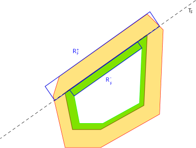
Figure 1. The external and internal rectangles associated to a face $F$ of a polygon. The external and internal morphological boundaries are respectively represented by the areas in yellow and green. The rectangles, $R_{F}^{+}$ and $R_{F}^{-}$, given by Fact Fact are drawn in blue.

This fact is illustrated on Figure 1 and its easy proof is left to the reader. We are now in a position to prove Proposition 7.

Proof of Proposition 7.

From the above fact and (3.3) there is $\epsilon=\epsilon^{-}(I,\angle J)>0$ and $C=C(I,\angle J)>0$ such that for any convex polytope $J=A_{1}\cdots A_{n}$

$$\sharp\underline{\partial^{-}J} \geq\sum_{l<n}\sharp\underline{R_{A_{l}(\epsilon)A_{l+1}(\epsilon)}\left(-h_{I}(N^{A_{l}A_{l+1}})\right)},$$

$$\geq\sum_{F\in\mathcal{F}(J)}\left[\sharp\underline{R_{F}\left(-h_{I}(N^{F})\right)}-C\right].$$

Then when $J$ is an integral convex polytope we get by Lemma 8 :

$$\sharp\underline{\partial^{-}J} \geq-C\sharp\mathcal{F}(J)+\sum_{F\in\mathcal{F}(J)}V\left(R_{F}\left(-h_{I}(N^{F})\right)\right),$$

$$\geq-C\sharp\mathcal{F}(J)+\int_{\mathbb{S}^{d}}h_{I}\,d\sigma_{J}.$$

For an integral convex exhaustion $(\mathsf{J}_{n})_{n}$ we obtain finally for large $n$ by using Lemma 7 and Lemma 6

$$\sharp\underline{\partial^{-}\mathsf{J}_{n}} \geq-C(I,\frac{\angle\mathsf{J}_{\infty}}{2})\cdot\sharp\mathcal{F}(\mathsf{J}_{n})+\int_{\mathbb{S}^{d}}h_{I}\,d\sigma_{\mathsf{J}_{n}},$$

$$\liminf_{n}\frac{\sharp\underline{\partial^{-}\mathsf{J}_{n}}}{p(\mathsf{J}_{n})} \geq\lim_{n}\int_{\mathbb{S}^{d}}h_{I}\,d\sigma_{\tilde{\mathsf{J}_{n}}},$$

$$\geq\int_{\mathbb{S}^{d}}h_{I}\,d\sigma_{\mathsf{J}_{\infty}}.$$

One proves similarly that $\limsup_{n}\frac{\sharp\underline{\partial^{+}\mathsf{J}_{n}}}{p(\mathsf{J}_{n})}\leq\int_{\mathbb{S}^{d}}h_{I}\,d\sigma_{\mathsf{J}_{\infty}}$ and this concludes the proof of Proposition 7 as we have $\sharp\underline{\partial^{+}\mathsf{J}_{n}}\geq\sharp\underline{\partial^{-}\mathsf{J}_{n}}$ according to Lemma 3. ∎

3.6. Supremum of $O\mapsto V_{I}(O)$

In this section we investigate the supremum of $V_{I}$ on $\mathcal{D}^{1}$ for a given convex polytope $I$ of $\mathbb{R}^{d}$. We recall that there is a unique sphere $S_{I}$ containing $I$ with minimal radius, usually called the smallest bounding sphere of $I$. We let $R_{I}$ and $x_{I}$ be respectively the radius and the center of $S_{I}$. There are at least two distinct points in $S_{I}\cap I$, whenever $I$ is not reduced to a singleton, and $S_{I}\cap I\subset\mathop{\mathrm{ex}}(I)$. Moreover we have the following alternative :

• either there is a finite subset of $S_{I}\cap I$ generating an inscribable polytope $T$ with $\mathop{\mathrm{Int}}(T)\ni x_{I}$ (in particular the interior set of $I$ is non empty),

• or there is a hyperplane $H$ containing $x_{I}$ such that $I$ lies in an associated semispace and $S_{I}\cap H$ is the smallest bounding sphere of $I\cap H$.

The smallest bounding sphere $S_{I}$ (or $I$ itself) will be said nondegenerated (resp. degenerated) and an associated polytope $T$ (resp. hyperplane $H$) is said generating. For an inscribable polytope $T$ in $\mathbb{R}^{d}$ we may define its dual $T^{\prime}$ as the polytope given by the intersection of the inner semispaces tangent to the circumsphere of $T$ at the vertices of $T$. In the following $T^{\prime}$ always denotes the dual polytope of a generating polytope $T$ with respect to $I$.

When $S_{I}$ is degenerated, there is a sequence of affine spaces $H=H_{1}\supset H_{2}\supset\cdots H_{l}\ni x_{I}$ such that $I\cap H_{l}$ is nondegenerated in $H_{l}$ and for all $1\leq i<l$ the convex polytope $I\cap H_{i}$ is degenerated in $H_{i}$ with $H_{i+1}$ as an associated generating hyperplane ($H_{i}$ is a $d-i$ dimensional affine space). We denote by $L$ a generating polytope of $I\cap H_{l}$ in $H_{l}$ and by $L^{\prime}$ its dual polytope in $H_{l}$. Let $U$ be an isometry of $\mathbb{R}^{d}$ mapping $H_{i}$ for $i=1,\cdots,l$ to $\{0_{i}\}\times\mathbb{R}^{d-i}$ (where $0_{i}$ denotes the origin of $\mathbb{R}^{i}$) with $U(x_{I})=0$. Then for $R>0$ we let $T^{\prime}_{R}:=U^{-1}\left([-R,R]^{l}\times U(L^{\prime})\right)$. The faces $F$ of $T^{\prime}_{R}$ satisfy

1. either $F=U^{-1}\left([-R,R]^{l}\times U(\mathsf{F})\right)$ for some face $\mathsf{F}$ of $L^{\prime}$,

2. or $F=U^{-1}\left([-R,R]^{l-1}\times\{\pm R\}_{i}\times U(L^{\prime})\right)$ for $i=1,\cdots,l$ (where $\{\pm R\}_{i}$ coresponds to the $i^{th}$ coordinate of the product).

For $i=1,2$ we let $\mathcal{F}_{i}(T^{\prime}_{R})$ be the subset of $\mathcal{F}(T^{\prime}_{R})$ given by the faces of the $i^{\text{th}}$ category.

Observe that when $x_{I}$ coincide with the origin then $T^{\prime}$ or $T^{\prime}_{R}$, $R>0$ are convex domains.

Proposition 8.

$$\sup_{O\in\mathcal{D}^{1}}V_{I}(O)=R_{I}.$$

The supremum of $V_{I}$ is achieved if and only if $S_{I}$ is nondegenerated. The supremum is then achieved for $O\in\mathcal{D}^{1}$ homothetic to the dual polytope $T^{\prime}$ of a generating polytope $T$.

Proof.

For any $v\in\mathbb{R}^{d}$ we have

$$V_{I+v}(O) =\int h_{I+v}\,d\sigma_{O},$$

$$=\int h_{I}\,d\sigma_{O}+\int_{\mathbb{S}^{d}}v\cdot u\,d\sigma_{O}(u),$$

$$=\int h_{I}\,d\sigma_{O}+\int_{\partial O}v\cdot N^{O}\,d\mathcal{H}_{d-1}.$$

By the divergence formula we have $\int_{\partial O}v\cdot N^{O}\,d\mathcal{H}_{d-1}=0$ for any $v\in\mathbb{R}^{d}$ and $O\in\mathcal{D}^{1}$. Therefore we may assume $x_{I}=0$. With the above notations we have $\max_{i\in I}i\cdot v\leq R_{I}$ for all $v\in\mathbb{R}^{d}$ with $\|v\|=1$ with equality iff $v$ belongs to $R_{I}^{-1}I$. Therefore $V_{I}(O)\leq R_{I}$ for any $O\in\mathcal{D}^{1}$. Moreover if the equality occurs then for $x$ in a subset $E$ of $\partial O$ with full $\mathcal{H}_{d-1}$-measure, $h_{I}\left(N^{O}(x)\right)=\max_{i\in I}i\cdot x=R_{I}$ and therefore the normal unit vector $N^{O}(x)$ belongs to $R_{I}^{-1}I$. But as $O$ is a convex domain, we may find $d+1$ points $x_{1},\cdots,x_{d+1}$ in $E$ in such a way the origin belongs to the interior of the simplex $T=R_{I}\mathop{\mathrm{cv}}\left(N^{O}(x_{1}),\cdots,N^{O}(x_{d+1})\right)$. Thus $S_{I}$ is nondegenerated and the polytope $T$ is a generating polytope with respect to $I$. Moreover we have with the above notations

$$\int h_{I}\,d\sigma_{T^{\prime}}=R_{I}p(T^{\prime}).$$

Therefore the homothetic polytope $O^{\prime}$ of $T^{\prime}$ with unit perimeter achieves the supremum of $V_{I}$. We consider now the degenerated case. With the above notations, we have $h_{I}(N^{F})=R_{I}$ for any $F\in\mathcal{F}_{1}(T^{\prime}_{R})$ (recall we assume $x_{I}=0$ without loss of generality). Moreover $\mathcal{H}_{d-1}\left(\bigcup_{F\in\mathcal{F}_{2}(T^{\prime}_{R})}F\right)=o(p(T^{\prime}_{R}))$ when $R$ goes to infinity. Therefore the renormalization $O_{R}\in\mathcal{D}^{1}$ of $T^{\prime}_{R}$ satisfies

$$V_{I}(O_{R})\xrightarrow{R\rightarrow+\infty}R_{I}.$$

∎

4. Cellular automata

4.1. Definitions

We consider a finite set $\mathcal{A}$. We endow the set $\mathcal{A}$ with the discrete topology and $X_{d}=\mathcal{A}^{\mathbb{Z}^{d}}$ with the product topology. We consider the $\mathbb{Z}^{d}$-shift $\sigma$ on $\mathcal{A}^{\mathbb{Z}^{d}}$ defined for $l\in\mathbb{Z}^{d}$ and $u=(u_{k})_{k}\in X_{d}$ by $\sigma^{l}(u)=(u_{k+l})_{k}$. Any closed subset $X$ of $X_{d}$ invariant under the action of $\sigma$ is called a $\mathbb{Z}^{d}$-subshift. We fix such a subshift $X$ in the remaining of the paper.

For a bounded subset $J$ of $\mathbb{R}^{d}$ we consider the partition $\mathsf{P}_{J}$ into $\underline{J}$-cylinders, i.e. the element $\mathsf{P}_{J}^{x}$ of $\mathsf{P}_{J}$ containing $x=(x_{i})_{i\in\mathbb{Z}^{d}}\in X$ is given by $\mathsf{P}_{J}^{x}:=\{y=(y_{i})_{i\in\mathbb{Z}^{d}}\in X,\ \forall i\in\underline{J}\ y_{i}=x_{i}\}$. In other terms we may define $\mathsf{P}_{J}$ as the joined partition $\bigvee_{j\in\underline{J}}\sigma^{-j}\mathsf{P}_{0}$ with $\mathsf{P}_{0}$ being the zero-coordinate partition.

A cellular automaton (CA for short) defined on a $\mathbb{Z}^{d}$-subshift $X$ is a continuous map $f:X\rightarrow X$ which commutes with the shift action $\sigma$. By a famous theorem of Hedlund [14] the cellular automaton $f$ is given by a local rule, i.e. there exists a finite subset $I$ of $\mathbb{Z}^{d}$ and a map $F:\mathcal{A}^{I}\rightarrow\mathcal{A}$ such that

$$\forall j\in\mathbb{Z}^{d}\ \left(fx\right)_{j}=F\left(\left(x_{j+i}\right)_{i\in I}\right).$$

The (smallest) subset $I$ is called the domain of the CA. Recall $I^{\prime}=I\cup\{0\}$ and let $\mathbb{I}$ be the convex hull of $I^{\prime}$.

4.2. Lyapunov exponents for higher dimensional cellular automata

Lyapunov exponent of one-dimensional cellular automata have been defined in [15, 16]. We develop a similar theory in higher dimensions. Let $f$ be a CA on a $\mathbb{Z}^{d}$-subshift $X$ with domain $I$.

Given a convex body $J$ of $\mathbb{R}^{d}$ and $x\in X$, we let

$$\mathcal{E}_{f}(x,J):=\{K\text{ convex body},\ f\mathsf{P}_{J}^{x}\subset\mathsf{P}_{K}^{fx}\}$$

A priori the family $\mathcal{E}_{f}(x,J)$ does not admit a greatest element for the inclusion. Observe also that the convex body $J\ominus I$ belongs to $\mathcal{E}_{f}(x,J)$, in particular this family is not empty. Then we let for all $x$ :

$${\mathop{\mathrm{gr}}}_{J}f(x):=\min\{\sharp\underline{J\setminus K},\ K\in\mathcal{E}_{f}(x,J)\}.$$

The family $\mathcal{E}_{f}(x,J)$ and the function ${\mathop{\mathrm{gr}}}_{J}f(x)$ are constant on each atom $A$ of $\mathsf{P}_{J}$, thus we let $\mathcal{E}_{f}(A,J)$ and ${\mathop{\mathrm{gr}}}_{J}f(A)$ be these quantities. We denote by $\mathcal{D}_{f}(x,J)$ the subfamily of $\mathcal{E}_{f}(x,J)$ consisting in $K$ with $\sharp\underline{J\setminus K}={\mathop{\mathrm{gr}}}_{J}f(x)$. For $K$ in $\mathcal{D}_{f}(x,J)$ the intersection $K\cap J$ defines a convex body, which belongs also to $\mathcal{D}_{f}(x,J)$.

For a convex exhaustion $\mathcal{J}=(J_{n})_{n}$, we define the growth ${\mathop{\mathrm{gr}}}_{\mathcal{J}}f$ with respect to $\mathcal{J}$ as the following real functions on $X$ :

$${\mathop{\mathrm{gr}}}_{\mathcal{J}}f:=\limsup_{n}\frac{{\mathop{\mathrm{gr}}}_{J_{n}}f}{p(J_{n})}.$$

Finally we let for a convex domain $O\in\mathcal{D}^{1}$ :

$${\mathop{\mathrm{gr}}}_{O}f=\sup_{\mathcal{J}\in\mathcal{E}(O)}{\mathop{\mathrm{gr}}}_{\mathcal{J}}f.$$

Lemma 9.

The sequence of functions $\left({\mathop{\mathrm{gr}}}_{O}f^{k}\right)_{k}$ is subadditive, i.e.

$$\forall k,l\in\mathbb{N}\ \forall x\in X,\ {\mathop{\mathrm{gr}}}_{O}f^{k+l}(x)\leq{\mathop{\mathrm{gr}}}_{O}f^{l}(f^{k}x)+{\mathop{\mathrm{gr}}}_{O}f^{k}(x).$$

Proof.

Fix $x\in X$ and $k,l\in\mathbb{N}$. Let $\mathcal{J}=(J_{n})_{n}\in\mathcal{E}(O)$. We consider a sequence $\mathcal{K}:=(K_{n})_{n}$ of convex bodies in $\prod_{n}\mathcal{D}_{f^{k}}(x,J_{n})$ with $K_{n}\subset J_{n}$ for all $n$. Let $I_{k}$ be the domain of $f^{k}$. The convex body $J_{n}\ominus I_{k}$ belongs to $\mathcal{E}_{f^{k}}(x,J_{n})$ for all $n$. By Proposition 5, we have $\sharp\underline{J_{n}\setminus K_{n}}\leq\sharp\underline{\partial_{I_{k}}^{-}J_{n}}=O\left(p(J_{n})\right)$. It follows from Lemma 1 and Remark 2 that $\mathcal{K}$ is a convex exhaustion in $\mathcal{E}(O)$ with $p(K_{n})\sim^{n}p(J_{n})$. We also let $\mathcal{L}=(L_{n})_{n}\in\prod_{n}\mathcal{D}_{f^{l}}(f^{k}x,K_{n})$ with $L_{n}\subset K_{n}$ for all $n$. Similarly the sequence $\mathcal{L}$ belongs to $\mathcal{E}(O)$ with $p(L_{n})\sim^{n}p(J_{n})$. Then we have for all positive integers $n$ :

$$f^{k+l}\mathsf{P}_{J_{n}}^{x} =f^{l}(f^{k}\mathsf{P}_{J_{n}}^{x}),$$

$$\subset f^{l}\left(\mathsf{P}_{K_{n}}^{f^{k}x}\right),$$

$$\subset\mathsf{P}_{L_{n}}^{f^{k+l}x}.$$

Therefore we have

$${\mathop{\mathrm{gr}}}_{J_{n}}f^{k+l}(x) \leq\sharp\underline{J_{n}\setminus L_{n}},$$

$$\leq\sharp\underline{J_{n}\setminus K_{n}}+\sharp\underline{K_{n}\setminus L_{n}},$$

then

$${\mathop{\mathrm{gr}}}_{\mathcal{J}}f^{k+l}(x) =\limsup_{n}\frac{{\mathop{\mathrm{gr}}}_{J_{n}}f}{p(J_{n})},$$

$$\leq\limsup_{n}\frac{{\mathop{\mathrm{gr}}}_{K_{n}}f}{p(J_{n})}+\limsup_{n}\frac{{\mathop{\mathrm{gr}}}_{L_{n}}f}{p(J_{n})},$$

$$\leq\limsup_{n}\frac{{\mathop{\mathrm{gr}}}_{K_{n}}f}{p(K_{n})}+\limsup_{n}\frac{{\mathop{\mathrm{gr}}}_{L_{n}}f}{p(L_{n})},$$

$$\leq{\mathop{\mathrm{gr}}}^{+}_{\mathcal{K}}f^{k}(x)+{\mathop{\mathrm{gr}}}^{+}_{\mathcal{L}}f^{l}(f^{k}x),$$

As the sequence $\mathcal{K}$ and $\mathcal{L}$ lie in $\mathcal{E}(O)$ we conclude that

$${\mathop{\mathrm{gr}}}_{O}f^{k+l}(x) \leq{\mathop{\mathrm{gr}}}_{O}f^{k}(x)+{\mathop{\mathrm{gr}}}_{O}f^{l}(f^{k}x).$$

∎

The nonnegative function ${\mathop{\mathrm{gr}}}_{O}f$ satisfies ${\mathop{\mathrm{gr}}}_{O}f\leq\sup_{\mathcal{J}\in\mathcal{E}(O)}\limsup_{n}\frac{\sharp\underline{\partial_{I}^{-}J_{n}}}{p\left(J_{n}\right)}$ and this last term is finite according to Proposition 5. Therefore the subadditive ergodic theorem applies : for any $\mu\in\mathcal{M}(X,f)$ the sequence $\left(\frac{1}{n}{\mathop{\mathrm{gr}}}_{O}f^{n}(x)\right)_{k}$ converge almost everywhere to a $f$-invariant function $\chi_{O}$ with $\int\chi_{O}\,d\mu=\lim/\inf_{n}\frac{1}{n}\int{\mathop{\mathrm{gr}}}_{O}f^{n}\,d\mu$. We call the function $\chi_{O}$ the Lyapunov exponent of $f$ with respect to $O$.

Remark 9.

The exponent $\chi_{O}$ for $O\in\mathcal{D}$ plays some how the role of the sum of the positive Lyapunov exponents in smooth dynamical systems.

5. Rescaled entropy of cellular automata

5.1. Definition

We let $\mathcal{M}(f)$ (resp. $\mathcal{M}(f,\sigma)$) be the set of invariant Borel probability measures on $X$ which are $f$-invariant (resp. $f$- and $\sigma$-invariant). For a finite clopen partition $\mathsf{P}$ of $X$ we let $H_{top}(\mathsf{P})=\log\sharp\mathsf{P}$ and $H_{\mu}(\mathsf{P})=-\sum_{A\in\mathsf{P}}\mu(A)\log\mu(A)$ with $\mu\in\mathcal{M}(f)$. In the following the symbol $*$ denotes either $*=top$ or $*=\mu\in\mathcal{M}(f)$. We let $h_{*}(f,\mathsf{P})$ be the entropy with respect to the clopen partition $\mathsf{P}$ :

$$h_{*}(f,\mathsf{P}):=\lim_{n}\frac{1}{n}H_{*}\left(\bigvee_{k=0}^{n-1}f^{-k}\mathsf{P}\right).$$

For two partitions $\mathsf{P}$, $\mathsf{Q}$ of $X$, we say $\mathsf{P}$ is finer than $\mathsf{Q}$ and we write $\mathsf{P}>\mathsf{Q}$, when any atom of $\mathsf{P}$ is contained in an atom of $\mathsf{Q}$. The functions $H_{*}(\cdot)$ and $h_{*}(f,\cdot)$ are nondecreasing with respect to this order.

The rescaled entropy with respect to a convex exhaustion $\mathcal{J}=(J_{n})_{n}$ is defined as follows

$$h^{d}_{*}(f,\mathcal{J})=\limsup_{n}\frac{h_{*}(f,\mathsf{P}_{J_{n}})}{p(J_{n})}.$$

In [9] the authors defines a similar notion for the rescaled topological entropy with the renormalization factor $\sharp\partial^{-}_{I}\underline{J_{n}}$ (which depends on the domain $I$ of $f$) rather than $p(J_{n})$.

Remark 10.

For $d=2$, when $J=\bigcup_{i\in I}J_{i}$ is a finite disjoint union of Jordan domains $J_{i}$ with Lipshitz boundary, we have

$$\frac{h_{top}(f,\mathsf{P}_{J})}{p(J)} \leq\frac{\sum_{i\in I}h_{top}(f,\mathsf{P}_{J_{i}})}{\sum_{i\in I}p(J_{i})},$$

$$\leq\sup_{i\in I}\frac{h_{top}(f,\mathsf{P}_{J_{i}})}{p(J_{i})}.$$

Moreover for each $i$, we have $p(J_{i})\geq p\left(\mathop{\mathrm{cv}}(J_{i})\right)$ and $\mathsf{P}_{\mathop{\mathrm{cv}}(J_{i})}$ is finer than $\mathsf{P}_{J_{i}}$. Therefore

$$\frac{h_{top}(f,\mathsf{P}_{J})}{p(J)} \leq\frac{\sum_{i\in I}h_{top}(f,\mathsf{P}_{J_{i}})}{\sum_{i\in I}p(J_{i})},$$

$$\leq\sup_{i\in I}\frac{h_{top}(f,\mathsf{P}_{\mathop{\mathrm{cv}}(J_{i})})}{p\left(\mathop{\mathrm{cv}}(J_{i})\right)}.$$

This inequality justifies somehow that we focus on convex bodies $J$ of $\mathbb{R}^{d}$.

We let also for any $O\in\mathcal{D}^{1}$

$$h^{d}_{*}(f,O)=\sup_{\mathcal{J}\in\mathcal{E}(O)}h^{d}_{*}(f,\mathcal{J})$$

and

$$h^{d}_{*}(f)=\sup_{\mathcal{J}}h^{d}_{*}(f,\mathcal{J}),$$

where the last supremum holds over all convex exhaustions $\mathcal{J}$. For $d=1$ we have $p(J)=2$ for any convex subset $J$. Therefore up to a factor $2$ we recover the usual definition of entropy, $2h^{1}_{*}(f)=h_{*}(f)$.

Remark 11.

As the CA $f$ commutes with the shift action $\sigma$ we have for all $k\in\mathbb{Z}^{d}$ and any subset $J$ of $\mathbb{Z}^{d}$ $h_{top}(f,\mathsf{P}_{J+k})=h_{top}(f,\sigma^{-k}\mathsf{P}_{J})=h_{top}(f,\mathsf{P}_{J})$ and the same holds for the measure theoretical entropy with respect to measures in $\mathcal{M}(f,\sigma)$. Let us call generalized convex domain any convex body with a non empty interior set. Replacing convex domains by generalized convex domains, we may define generalized convex exhaustions $\mathcal{J}$ and the associated rescaled entropies. Then it follows from the aforementioned invariance by translation of the entropy, that $h^{d}_{top}(O)=h^{d}_{top}(O+\alpha)$ for all $\alpha\in\mathbb{R}^{d}$ and all generalized convex domain $O$ with unit perimeter. Indeed for any $(J_{n})_{n}\in\mathcal{E}(O)$ (resp. $\mathcal{E}\left(\mathcal{O+\alpha}\right)$) there is a sequence of integers $(k_{n})_{n}$ with $(J_{n}+k_{n})_{n}\in\mathcal{E}\left(\mathcal{O+\alpha}\right)$ (resp. $(J_{n})_{n}\in\mathcal{E}(O)$).

Remark 12.

1. The partition $\mathsf{P}_{J_{n}}$ may be written as $\bigvee_{k\in J_{n}}\sigma^{-k}\mathsf{P}_{0}$ with $\mathsf{P}_{0}$ being the zero-coordinate partition. Instead of $\mathsf{P}_{0}$ we could choose another clopen generating partition $\mathsf{P}$, i.e. a partition of $X$ into clopen sets with $\bigvee_{k\in\mathbb{Z}^{d}}\sigma^{-k}\mathsf{P}$ equal to the partition of $X$ into points. But for a finite subset $J$ of $\mathbb{Z}^{d}$ we have $\bigvee_{k\in J}\sigma^{-k}\mathsf{P}>\mathsf{P}_{0}$ and $\bigvee_{k\in J}\sigma^{-k}\mathsf{P}_{0}>\mathsf{P}$ so that in the definition of the rescaled entropy we may replace $\mathsf{P}_{0}$ by any other generator $\mathsf{P}$ of $X$, i.e. $\mathsf{P}_{J_{n}}$ by $\bigvee_{k\in\underline{J_{n}}}\sigma^{-k}\mathsf{P}$.

2. Let $X$ be a zerodimensional compact metrizable space endowed with a expansive $\mathbb{Z}^{d}$-action $\tau$. We consider a map $f$ preserving $(X,\tau)$ i.e. $f$ is an homeomorphism of $X$ commuting with $\tau$. The triple $(X,\tau,f)$ is called a topological $\mathbb{Z}^{d}$-expansive preserving system (t.e.p.s. for short). Two t.e.p.s. $(Y,\phi,g)$ are conjugated when there is a homeomorphism $h:X\rightarrow Y$ such that $h\circ f\circ h^{-1}=g$ and $h\circ\tau\circ h^{-1}=\phi$. We may define the rescaled entropy as we did for a CA and all the previous results hold in this more general setting. Moreover two conjugated t.e.p.s. have the same rescaled entropy. Any t.e.p.s. is conjugated to a CA.

5.2. Link with the metric mean dimension

In a compact metric space $(X,\mathsf{d})$, the ball of radius $\epsilon\geq 0$ centered at $x\in X$ will be denoted by $B_{\mathsf{d}}(x,\epsilon)$. For a continuous map $f:X\rightarrow X$ we denote by $\mathsf{d}_{n}$ the dynamical distance defined for all $n\in\mathbb{N}$ by

$$\forall x,y\in X,\ \mathsf{d}_{n}(x,y)=\max\{\mathsf{d}(f^{k}x,f^{k}y),\ 0\leq k<n\}.$$

The metric mean dimension of $f$ is defined as $\mathop{\mathrm{mdim}}(f,\mathsf{d})=\limsup_{\epsilon\rightarrow 0}\frac{h_{top}(f,\epsilon)}{|\log\epsilon|}$ where $h_{top}(f,\epsilon)$ denotes the topological entropy at the scale $\epsilon>0$ :

$$h_{top}(f,\epsilon):=\limsup_{n}\frac{1}{n}\log\min\{\sharp C,\ \bigcup_{x\in C}B_{\mathsf{d}_{n}}(x,\epsilon)=X\}.$$

The topologial mean dimension is the infimum of $\mathop{\mathrm{mdim}}(f,\mathsf{d})$ over all distances on $X$. We refer to [11] for alternative definitions and furter properties of mean dimension. The topological mean dimension of a finite dimensional topological system is null.

Here $f$ is a CA on a subshift of $\mathbb{Z}^{d}$. In particular it has zero topological mean dimension. For a norm $\|\cdot\|$ of $\mathbb{R}^{d}$ we may associate a metric $\mathsf{d}_{\|\|}$ on $X_{d}$ by letting $\mathsf{d}_{\|\|}(u,v)=\alpha^{-\min\{\|k\|,\ k\in\mathbb{Z}^{d},\ u_{k}\neq v_{k}\}}$ for all $u=(u_{k})_{k},v=(v_{k})_{k}\in X_{d}$. Then for $l\in\mathbb{N}$ the (open) ball $B_{\mathsf{d}_{\|\|}}(x,2^{-l})$ with respect to $\mathsf{d}_{\|\|}$ coincides with the cylinder $\mathsf{P}_{J_{l}}^{x}$ with $J_{l}=B_{\|\|}(0,l)$.

As there is a correspondence between convex symmetric domains and unit balls of norms on $\mathbb{R}^{d}$, the mean dimension with respect to such distances $\mathsf{d}_{\|\|}$ are given by $h_{top}^{d}(f,\mathcal{J}_{O})$ for convex symmetric domains $O$.

Remark 13.

In [17] the authors work with a measure theoretical quantity, called the measure distorsion rate dimension and show a variational principle with the metric mean dimension of $d_{\|\|}$. Does this quantity coincides with $\mu\mapsto h^{d}_{\mu}(f,O)$ with $O$ being the symmetric convex domain associated to the norm $\|\|$?

5.3. Monotonicity and Power

We investigate now basic properties of the rescaled entropy.

Lemma 10.

For any $O\in\mathcal{D}$ and any $\alpha>0$, we have

$$h^{d}_{*}(f,\mathcal{J}_{O})=h^{d}_{*}(f,\mathcal{J}_{\alpha O}).$$

Proof.

For $n\in\mathbb{N}$, we let $k_{n}=\lceil\frac{n}{\alpha}\rceil$, thus $nO\subset k_{n}\alpha O$ and $p(nO)\sim^{n}p(k_{n}\alpha O)$. Therefore

$$h^{d}_{*}(f,\mathcal{J}_{O}) =\limsup_{n}\frac{h_{*}(f,\mathsf{P}_{nO})}{p(nO)},$$

$$\leq\limsup_{n}\frac{h_{*}(f,\mathsf{P}_{k_{n}\alpha O})}{p(nO)},$$

$$\leq\limsup_{n}\frac{h_{*}(f,\mathsf{P}_{k_{n}\alpha O})}{p(k_{n}\alpha O)},$$

$$\leq h^{d}_{*}(f,\mathcal{J}_{\alpha O}).$$

The other inequality is obtained by considering $\alpha O$ and $\alpha^{-1}$ in place of $O$ and $\alpha$. ∎

Lemma 11.

For any $O\in\mathcal{D}^{1}$ and $O^{\prime}\in\mathcal{D}$ with $O\subset\mathop{\mathrm{Int}}(O^{\prime})$, we have

$$h^{d}_{*}(f,\mathcal{J}_{O})\leq h^{d}_{*}(f,O)\leq p(O^{\prime})h^{d}_{*}(f,\mathcal{J}_{O^{\prime}}).$$

Proof.

As $\mathcal{J}_{O}\in\mathcal{E}(O)$ the inequality $h^{d}_{*}(f,\mathcal{J}_{O})\leq h^{d}_{*}(f,O)$ follows from the definitions. Let now $\mathcal{J}\in\mathcal{E}(O)$. For $n$ large enough we have $\tilde{J}_{n}\subset\mathop{\mathrm{Int}}(O^{\prime})$, therefore $J_{n}\subset p(J_{n})^{\frac{1}{d-1}}O^{\prime}$. Therefore we conlude that

$$h^{d}_{*}(f,\mathcal{J}) \leq\limsup_{n}\frac{p\left(p(J_{n})^{\frac{1}{d-1}}O^{\prime}\right)}{p(J_{n})}h^{d}_{*}(f,\mathcal{J}_{O^{\prime}}),$$

$$\leq p(O^{\prime})h^{d}_{*}(f,\mathcal{J}_{O^{\prime}}).$$

∎

For $O\in\mathcal{D}^{1}$ the origin belongs to $\mathop{\mathrm{Int}}(O)$ so that $\alpha O\in\mathcal{D}$ and $O\subset\mathop{\mathrm{Int}}(\alpha O)$ for any $\alpha>1$. Moreover we have $h^{d}_{*}(f,\mathcal{J}_{\alpha O})=h^{d}_{*}(f,\mathcal{J}_{O})$ by Lemma 10. Together with Lemma 11 we get immediately :

Corollary 14.

$$\forall O\in\mathcal{D}^{1},\ h^{d}_{*}(f,O)=h^{d}_{*}(f,\mathcal{J}_{O}).$$

Corollary 15.

$$O\mapsto h_{*}^{d}(f,O)\text{ is continuous on }\mathcal{D}^{1}.$$

Convex polytopes are dense in $\mathcal{D}$. Therefore we get with $\mathcal{P}$ being the collections of convex $d$-polytopes with the origin in their interior set :

Corollary 16.

$$\sup_{O\in\mathcal{D}^{1}}h^{d}_{*}(f,O)=\sup_{P\in\mathcal{P}}h^{d}_{*}(f,\mathcal{J}_{P}).$$

However we will see that the supremum is not always achieved. We prove now a formula for the rescaled entropy of a power.

Lemma 12.

$$\forall O\in\mathcal{D}^{1}\ \forall k\in\mathbb{N},\ h^{d}_{*}(f^{k},O)=kh^{d}_{*}(f,O).$$

Proof.

Let $O\in\mathcal{D}^{1}$ and $\mathcal{J}=(J_{n})_{n}\in\mathcal{E}(O)$. Let $J_{n}^{k}=J_{n}\oplus\underbrace{I\oplus\cdots\oplus I}_{k\text{ times}}$ for all $n$. The sequence $\mathcal{J}^{k}=(J_{n}^{k})_{n}$ belongs also to $\mathcal{E}(O)$. Moreover the partition $\mathsf{P}_{J_{n}^{k}}$ is finer than $\bigvee_{l=0}^{k-1}f^{-l}\mathsf{P}_{J_{n}}$. Therefore

$$h_{*}(f^{k},\mathsf{P}_{J_{n}})\leq kh_{*}(f,\mathsf{P}_{J_{n}})=h_{*}\left(f^{k},\bigvee_{l=0}^{k-1}f^{-l}\mathsf{P}_{J_{n}}\right)\leq h_{*}(f^{k},\mathsf{P}_{J_{n}^{k}})$$

and we then obtain

$$h_{*}^{d}(f^{k},\mathcal{J})\leq kh_{*}^{d}(f,\mathcal{J})\leq h_{*}^{d}(f^{k},\mathcal{J}^{k}).$$

We conclude by taking the supremum in $\mathcal{J}\in\mathcal{E}(O)$. ∎

Remark 17.

Clearly we have $h^{d}_{\mu}\leq h^{d}_{top}$ for any $\mu\in\mathcal{M}(f)$ but we ignore if a general variational principle holds true.

5.4. A first upperbound for the rescaled entropy

Let $(X,f)$ be a cellular automaton with domain $I$. We relate the entropy of $\mathsf{P}_{J}$ with the entropy of $\mathsf{P}_{\partial^{\pm}J}$ and we prove an upperbound for the rescaled entropy $h_{top}^{d}(f,O)$ in term of the first relative quermass integral $V_{\mathbb{I}}(O)$ with $\mathbb{I}$ being the convex hull of $I^{\prime}$.

Lemma 13.

For any bounded subset $J$ of $\mathbb{R}^{d}$, we have

$$h_{*}(f,\mathsf{P}_{J})=h_{*}(f,\mathsf{P}_{\partial_{I}^{-}J})\text{ and }h_{*}(f,\mathsf{P}_{J})\leq h_{*}(f,\mathsf{P}_{\partial_{I}^{+}J}).$$

Proof.

The inequality $h_{*}(f,\mathsf{P}_{J})\geq h_{*}(f,\mathsf{P}_{\partial_{I}^{-}J})$ follows directly from the inclusion $\partial^{-}J\subset J$. By definition of the domain $I$ and the erosion $J\ominus I$, we have $P_{J}>f^{-1}P_{J\ominus I}$. Therefore we get $f^{-1}\mathsf{P}_{J}\vee\mathsf{P}_{J}=f^{-1}\mathsf{P}_{\partial^{-}J}\vee P_{J}$ and then by induction $\mathsf{P}_{J}\vee\bigvee_{l=0}^{k-1}f^{-l}\mathsf{P}_{\partial^{-}J}=\bigvee_{l=0}^{k-1}f^{-l}\mathsf{P}_{J}$ for all $k$. We conclude that :

$$h_{*}(f,\mathsf{P}_{J}) =\lim_{k}\frac{1}{k}H_{*}(f,\bigvee_{l=0}^{k-1}f^{-l}\mathsf{P}_{J}),$$

$$\leq\lim_{k}\frac{1}{k}\left(H_{*}\left(\mathsf{P}_{J}\right)+H_{*}\left(\bigvee_{l=0}^{k-1}f^{-l}\mathsf{P}_{\partial^{-}J}\right)\right),$$

$$\leq h_{*}(f,\mathsf{P}_{\partial^{-}J}).$$

We also have

$$\mathsf{P}_{J}\vee\mathsf{P}_{\partial^{+}J}>\mathsf{P}_{J\oplus I}>f^{-1}\mathsf{P}_{J}.$$

Therefore we get now by induction on $k$

$$\mathsf{P}_{J}\vee\bigvee_{l=0}^{k-2}f^{-l}\mathsf{P}_{\partial^{+}J}>\bigvee_{l=0}^{k-1}f^{-l}\mathsf{P}_{J}.$$

This implies $h_{*}(f,\mathsf{P}_{\partial_{I}^{+}J})\leq h_{*}(f,\mathsf{P}_{J})$.

∎

Proposition 18.

For any $O\in\mathcal{D}^{1}$,

$$h^{d}_{top}(f,O)\leq V_{\mathbb{I}}(O)\log\sharp\mathcal{A}.$$

Proof.

Recall that

$$h^{d}_{top}(f,O) =h^{d}_{top}(f,\mathcal{J}_{O}),$$

$$=\limsup_{n}\frac{h_{top}(f,\mathsf{P}_{nO})}{p(nO)}.$$

Then by applying Lemma 13 we obtain

$$h^{d}_{top}(f,O) \leq\limsup_{n}\frac{h_{top}(f,\mathsf{P}_{\partial^{\pm}nO})}{p(nO)},$$

$$\leq\limsup_{n}\frac{\sharp\underline{\partial^{\pm}nO}\log\sharp\mathcal{A}}{p(nO)}.$$

For all $k\in\mathbb{N}\setminus\{0\}$ we let $I_{k}$ be the domain of $f^{k}$ and we denote by $\mathbb{I}_{k}$ the convex hull of $I^{\prime}_{k}=I_{k}\cup\{0\}$. Clearly we have $I_{k}\subset\underbrace{I\oplus\cdots\oplus I}_{k\text{ times }}$, therefore $\mathbb{I}_{k}\subset k\mathbb{I}$. By Lemma 4, we get for some constant $C=C(d)$ :

$$h^{d}_{top}(f^{k},O) \leq\left(V_{\mathbb{I}_{k}}(O)+C\right)\log\sharp\mathcal{A},$$

$$\leq\left(V_{k\mathbb{I}}(O)+C\right)\log\sharp\mathcal{A},$$

$$\leq\left(kV_{\mathbb{I}}(O)+C\right)\log\sharp\mathcal{A}.$$

But by Lemma 16 we have $h^{d}_{top}(f^{k},O)=kh^{d}_{top}(f,O)$, so that we finally conclude when $k$ goes to infinity

$$h^{d}_{top}(f,O)\leq V_{\mathbb{I}}(O)\log\sharp\mathcal{A}.$$

∎

6. Ruelle inequality

Recall $(X,\sigma)$ denotes a $\mathbb{Z}^{d}$-subshift. The topological entropy of $\sigma$ is defined for any Fölner sequence $\mathcal{L}=(L_{n})_{n}$ (see e.g. [19]) as

$$h_{top}(\sigma)=\limsup_{n}\frac{H_{top}(\mathsf{P}_{L_{n}})}{\sharp L_{n}}.$$

Lemma 14.

For all $\epsilon>0$ there exists $c>0$ such that we have for any $K\subset J$ convex bodies:

$$H_{top}(\mathsf{P}_{J\setminus K})\leq\left(\sharp\underline{J\setminus K}+cp(J\oplus\mathsf{C})\right)\cdot(h_{top}(\sigma)+\epsilon).$$

Proof.

Let $\epsilon>0$. As the sequence of cubes $\mathcal{C}=(C_{n})_{n}$ defined by $C_{n}=[-n,n[^{d}\cap\mathbb{Z}^{d}$ is a Fölner sequence, there is a positive integer $m$ such that $\frac{H_{top}\left(\mathsf{P}_{C_{m}}\right)}{\sharp C_{m}}<h_{top}(\sigma)+\epsilon$. Then for some $c=c(m)>0$ we may cover $\underline{J\setminus K}$ by a family $\mathcal{F}$ at most $\frac{\sharp\underline{J\setminus K}+cp(J\oplus\mathsf{C})}{\sharp C_{m}}$ disjoint translated copies of $C_{m}$. Indeed if $\mathsf{R}_{m}$ denotes a partition of $\mathbb{R}^{d}$ into translated copies of $C_{m}$, then any atom $A$ of $\mathsf{R}_{m}$ with $\underline{A}\cap\left(J\setminus K\right)\neq\emptyset$ either satisfies $\underline{A}\subset J\setminus K$ or $\underline{A}\cap\left(\partial^{-}_{C_{m}}J\cup\partial^{-}_{C_{m}}K\right)\neq\emptyset$. Clearly the number of $A$’s in the first case is less than $\frac{\sharp\underline{J\setminus K}}{\sharp C_{m}}$, whereas the numbers of atoms $A$ satisfying the second condition is less than $\sharp\underline{\partial^{-}_{C_{m}}J}+\sharp\underline{\partial^{-}_{C_{m}}K}$. Arguing as in the proof of Proposition 5, this last term is less than $c\left(p(J\oplus\mathsf{C})+p(K\oplus\mathsf{C})\right)$ for some constant $c$ depending on $m$. As $K$ is contained in $J$ we have $p(J\oplus\mathsf{C})\leq p(K\oplus\mathsf{C})$.

Therefore

$$H_{top}(\mathsf{P}_{J\setminus K}) \leq\left(\sharp\underline{J\setminus K}+2cp(J\oplus\mathsf{C})\right)\frac{H_{top}\left(\mathsf{P}_{C_{m}}\right)}{\sharp C_{m}},$$

$$\leq\left(\sharp\underline{J\setminus K}+2cp(J\oplus\mathsf{C})\right)\cdot(h_{top}(\sigma)+\epsilon).$$

∎

We refine now the inequality obtained in Lemma 18 at the level of invariant measures :

Lemma 15.

$$\forall\mu\in\mathcal{M}(f),\ h_{\mu}(f,O)\leq h_{top}(\sigma)\int\chi_{O}\,d\mu.$$

Proof.

For any convex domain $J$ and any $\mu\in\mathcal{M}(f)$ we have

$$h_{\mu}(f,\mathsf{P}_{J}) \leq H_{\mu}(f^{-1}\mathsf{P}_{J}|\mathsf{P}_{J}),$$

$$\leq\sum_{A\in\mathsf{P}_{J}}\mu(A)H_{\mu_{A}}(f^{-1}\mathsf{P}_{J}).$$

Fix $\epsilon>0$ and let $c$ be as in Lemma 14. Then if $(K_{A})_{A\in\mathsf{P}_{J}}$ is a family of convex bodies in $\prod_{A\in\mathsf{P}_{J}}\mathcal{E}_{f}(A,J)$ with $K_{A}\subset J$ for all $A$ we obtain

$$h_{\mu}(f,\mathsf{P}_{J}) \leq\sum_{A\in\mathsf{P}_{J}}\mu(A)H_{\mu_{A}}(f^{-1}\mathsf{P}_{J\setminus K_{A}}),$$

$$\leq\sum_{A\in\mathsf{P}_{J}}\mu(A)H_{top}(\mathsf{P}_{J\setminus K_{A}}),$$

$$\leq\sum_{A\in\mathsf{P}_{J}}\mu(A)\left(\sharp\underline{J\setminus K_{A}}+cp(J\oplus\mathsf{C})\right)\cdot(h_{top}(\sigma)+\epsilon).$$

By choosing $K_{A}$ with $\sharp\underline{J\setminus K_{A}}$ minimal we obtain

$$h_{\mu}(f,\mathsf{P}_{J}) \leq\left(h_{top}(\sigma)+\epsilon\right)\cdot\left(\int{\mathop{\mathrm{gr}}}_{J}f\,d\mu+cp(J\oplus\mathsf{C})\right).$$

Therefore we have for any convex exhaustion $\mathcal{J}=(J_{n})_{n}$ (recall that $p(J_{n}\oplus\mathsf{C})\sim^{n}p(J_{n})$) :

$$h^{d}_{\mu}(f,\mathcal{J}) =\limsup_{n}\frac{h_{\mu}(f,\mathsf{P}_{J})}{p(J_{n})},$$

$$\leq\left(h_{top}(\sigma)+\epsilon\right)\cdot\left(\limsup_{n}\int\frac{{\mathop{\mathrm{gr}}}_{J_{n}}f}{p(J_{n})}\,d\mu+c\right).$$

By Proposition 5 we have for all $x\in X$

$$\sup_{n\in\mathbb{N}}\frac{{\mathop{\mathrm{gr}}}_{J_{n}}f(x)}{p(J_{n})}\leq\sup_{n\in\mathbb{N}}\frac{\sharp\underline{\partial^{-}J_{n}}}{p(J_{n})}<+\infty.$$

We may therefore apply Fatou’s Lemma to the sequence of functions $\left(-\frac{{\mathop{\mathrm{gr}}}_{J_{n}}f}{p(J_{n})}\right)_{n}$ :

$$\limsup_{n}\int\frac{{\mathop{\mathrm{gr}}}_{J_{n}}f}{p(J_{n})}\,d\mu\leq\int\limsup_{n}\frac{{\mathop{\mathrm{gr}}}_{J_{n}}f}{p(J_{n})}\,d\mu,$$

then

$$h^{d}_{\mu}(f,\mathcal{J}) \leq\left(h_{top}(\sigma)+\epsilon\right)\left(\int{\mathop{\mathrm{gr}}}_{\mathcal{J}}f\,d\mu+c\right).$$

By taking the supremum over $\mathcal{J}\in\mathcal{E}(O)$ we get

$$h^{d}_{\mu}(f,O) \leq\left(h_{top}(\sigma)+\epsilon\right)\left(\int{\mathop{\mathrm{gr}}}_{O}f\,d\mu+c\right).$$

By Lemma 12 we have $\frac{h^{d}_{\mu}(f^{k},O)}{k}=h^{d}_{\mu}(f,O)$ for any $k$. Apply the above inequality to $f^{k}$ :

$$h^{d}_{\mu}(f,O) \leq\left(h_{top}(\sigma)+\epsilon\right)\left(\int\frac{{\mathop{\mathrm{gr}}}_{O}f^{k}}{k}\,d\mu+\frac{c}{k}\right).$$

When $k$ goes to infinity and then $\epsilon$ goes to zero, we conclude $h^{d}_{\mu}(f,O)\leq h_{top}(\sigma)\int\chi_{O}\,d\mu$.

∎

7. Entropy formula for permutative CA

The cellular automaton $f$ is said permutative at $i\in\mathbb{Z}^{d}$ if for all pattern $P$ on $I\setminus\{i\}$ and for all $a\in\mathcal{A}$ there is $b\in\mathcal{A}$ such that the pattern $P^{i}_{b}$ on $I\cup\{i\}$ given by the completion of $P$ at $i$ by $b$ satisfies $F(P^{i}_{b})=a$, in particular $i$ belongs to the domain $I$ of $f$. The CA is said permutative when it is permutative at the nonzero extreme points of the convex hull $\mathbb{I}$ of $I^{\prime}=I\cup\{0\}$ (these points lie in $I$). The algebraic CA as described in the introduction are permutative.

Proposition 19.

The topological rescaled entropy of a permutative CA $f$ on $X_{d}$ is given by

$$h^{d}_{top}(f)=R_{I^{\prime}}\log\sharp\mathcal{A}.$$

The sets $I^{\prime}$ and $\mathbb{I}$ have the same smallest bounding sphere, thus $R_{I^{\prime}}=R_{\mathbb{I}}$. Theorem 1, stated in the introduction, follows from Proposition 19.

Question.

For a permutative CA, the uniform measure $\lambda^{\mathbb{Z}^{d}}$ with $\lambda$ being the uniform measure on $\mathcal{A}$ is known to be invariant [20]. Does the uniform measure maximize the entropy ?

Recall that for any $k\in\mathbb{N}\setminus\{0\}$ we denote by $I_{k}$ the domain of $f^{k}$ and $\mathbb{I}_{k}$ the convex hull of $I^{\prime}_{k}=I_{k}\cup\{0\}$. In the following we also let $C(P,L)=\{(x_{i})_{i\in\mathbb{Z}^{d}}\in X,\ x_{j}=p_{j}\,\forall j\in L\}$ be the cylinder associated to the pattern $P=(p_{j})_{j\in L}\in\mathcal{A}^{L}$ on $L\subset\mathbb{Z}^{d}$. We also write $C(P)$ for this cylinder when there is no confusion on $L$.

Lemma 16.

For any permutative CA $f$ and any $k\in\mathbb{N}\setminus\{0\}$, the CA $f^{k}$ is also permutative and

$$\mathbb{I}_{k}=k\mathbb{I}.$$

Proof.

As already observed, the inclusion $\mathbb{I}_{k}\subset k\mathbb{I}$ holds for any CA (not necessarily permutative). We will show $k\mathop{\mathrm{ex}}(\mathbb{I})\subset I^{\prime}_{k}$, which implies together with $\mathbb{I}_{k}\subset k\mathbb{I}$ the equality $\mathbb{I}_{k}=k\mathbb{I}$. Let $i\in\mathop{\mathrm{ex}}(\mathbb{I})\setminus\{0\}\subset I$. For a fixed $k$ we prove by induction on $k$ that $f^{k}$ is permutative at $ki$, in particular $ki\in I^{\prime}_{k}$. Let $P$ be a pattern on $I_{k}\setminus\{ki\}$ and let $a\in\mathcal{A}$. Since we have $I_{k}\subset I_{k-1}\oplus I$, we may complete $P$ by a pattern $Q$ on $\left(I_{k-1}\oplus I\right)\setminus\{ki\}$. By induction hypothesis, $(k-1)i$ lies in $\mathop{\mathrm{ex}}(\mathbb{I}_{k-1})$ and $i$ lies in $\mathop{\mathrm{ex}}(\mathbb{I})$, therefore $ki$ does not belong to $I_{k-1}\oplus\left(I\setminus\{i\}\right)$, so that we have $I_{k-1}\oplus\left(I\setminus\{i\}\right)\subset\left(I_{k-1}\oplus I\right)\setminus\{ki\}$. Therefore there is a pattern $R$ on $I\setminus\{i\}$ such that $f^{k-1}C\left(Q,\left(I_{k-1}\oplus I\right)\setminus\{ki\}\right)$ is contained in the cylinder $C(R,I\setminus\{i\})$. As $f$ is permutative at $i$ there is $b\in\mathcal{A}$ with $F(R_{b}^{i})=a$ or in other terms $f\left(C(R_{b}^{i},I)\right)\subset C\left(a,\{0\}\right)$. Since $f^{k-1}$ is permutative at $(k-1)i$, we may find $c\in\mathcal{A}$ with $f^{k-1}\left(C(Q^{ki}_{c},I_{k-1}\oplus I)\right)\subset C\left(b,\{i\}\right)$. Therefore we get

$$f^{k}\left(C(Q^{ki}_{c},I_{k-1}\oplus I)\right)\subset f\left(C(R^{i}_{b},I)\right)\subset C\left(a,\{0\}\right).$$

But $I_{k}$ is the domain of $f^{k}$ and $P$ is the restriction of $Q$ to $I_{k}\setminus\{ki\}$, so that we also have $f^{k}\left(C(P^{ki}_{c},I_{k})\right)\subset C\left(a,\{0\}\right)$, i.e. $f^{k}$ is permutative at $ki$. ∎

For a convex $d$-polytope $J$ and a face $F$ of $J$ we consider the subset of $\partial_{\mathbb{I}}^{-}J$ given by $\partial^{-}_{\mathbb{I}}F:=\partial_{\mathbb{I}}^{-}J\cap T_{F}^{+}J(-h_{\mathbb{I}}(N^{F}))$. The sets $\partial^{-}_{\mathbb{I}}F$ for $F\in\mathcal{F}(J)$ are covering $\partial^{-}_{\mathbb{I}}J$ but do not define a partition in general. For any $F\in\mathcal{F}(J)$ we let $u^{F}\in\mathop{\mathrm{ex}}(\mathbb{I})\subset I^{\prime}$ with $u^{F}\cdot N^{F}=h_{\mathbb{I}}(N^{F})$ and we also let $d_{F}$ be the the Euclidean distance to $T_{F}$. Then for $j\in\underline{\partial^{-}_{\mathbb{I}}J}$ we let $F_{j}$ be a face of $J$ such that $d_{F_{j}}(j+u^{F_{j}})=-d_{F_{j}}(j)+u^{F_{j}}\cdot N^{F_{j}}$ is maximal among faces $F$ with $j\in\partial^{-}_{\mathbb{I}}{F}$. We consider then a total order $\prec$ on $\underline{\partial^{-}_{\mathbb{I}}J}$ such that $i\prec j$ if $d_{F_{i}}(i+u^{F_{i}})<d_{F_{j}}(j+u^{F_{j}})$. We also let $\mathcal{F}_{\mathbb{I}}(J)$ be the subset of $\mathcal{F}(J)$ given by faces $F$ for which $u_{F}$ is uniquely defined. We denote by $\partial_{\mathbb{I}}^{\bot}J$ the subset of $\partial^{-}_{\mathbb{I}}J$ given by

$$\partial_{\mathbb{I}}^{\bot}J:=\bigcup_{F\in\mathcal{F}_{\mathbb{I}}(J)}\partial^{-}_{\mathbb{I}}F.$$

Lemma 17.

With the above notations, let $j\in\underline{\partial_{\mathbb{I}}^{\bot}J}$. Then

$$\forall k\in\mathbb{N},\ j+ku^{F_{j}}\notin\{j^{\prime},\,j^{\prime}\prec j\}\oplus k\mathbb{I}.$$

Proof.

We argue by contradiction : there are $j^{\prime}\prec j$ and $u\in\mathbb{I}$ with $j+ku^{F_{j}}=j^{\prime}+ku$. Observe that

$$d_{F_{j}}(j+ku^{F_{j}}) =d_{F_{j}}(j+u^{F_{j}})+(k-1)u^{F_{j}}\cdot N^{F_{j}},$$

$$d_{F_{j}}(j^{\prime}+ku) =d_{F_{j}}(j^{\prime}+u)+(k-1)u\cdot N^{F_{j}}.$$

We will show that the equality between these two distances implies $u=u^{F_{j}}$, therefore $j=j^{\prime}$. Indeed we have

$$d_{F_{j}}(j^{\prime}+u) \leq\sup_{v\in\mathop{\mathrm{ex}}(\mathbb{I})}d_{F_{j}}(j^{\prime}+v), u\cdot N^{F_{j}} \leq\sup_{v\in\mathop{\mathrm{ex}}(\mathbb{I})}v\cdot N^{F_{j}},$$

$$\leq d_{F_{j^{\prime}}}(j^{\prime}+u^{F_{j^{\prime}}}), \leq h_{\mathbb{I}}(N^{F_{j}}),$$

$$d_{F_{j}}(j^{\prime}+u) \leq d_{F_{j}}(j+u^{F_{j}}) u\cdot N^{F_{j}} \leq u^{F_{j}}\cdot N^{F_{j}},$$

therefore $u\cdot N^{F_{j}}=u^{F_{j}}\cdot N^{F_{j}}$, and finally $u=u^{F_{j}}$ as $j$ belongs to $\underline{\partial_{\mathbb{I}}^{\bot}J}$. ∎

For a partition $\mathsf{P}$ of $X$ and a positive integer $k$, we write $\mathsf{P}^{k}$ to denote the iterated partition $\bigvee_{l=0}^{k-1}f^{-l}\mathsf{P}$ in order to simplify the notations.

Lemma 18.

Let $J$ be a convex $d$-polytope and let $k,n$ be positive integers. For any $A^{k}\in\mathsf{P}_{J}^{k}$ and any pattern $P$ on $\underline{\partial^{\bot}_{\mathbb{I}}J}$, there is $w\in A^{k}$ such that $f^{k}w$ belongs to $C(P,\underline{\partial^{\bot}_{\mathbb{I}}J})$.

Proof.

For any $j\in\partial^{\bot}_{\mathbb{I}}J$ we let $P_{j}$ be the restriction of $P=(p_{l})_{l\in\partial^{\bot}J}$ to $\{j^{\prime},\,j^{\prime}\prec j\}$. We show now by induction on $j\in\underline{\partial^{\bot}J}$ that there is $w\in A^{k}$ with $f^{k}w\in C(P_{j})$. By Lemma 16 the CA $f^{k}$ is permutative at $ku^{F_{j}}$ so that we may change the $(j+ku^{F_{j}})^{\text{th}}$-coordinate of $w$ to get $w^{\prime}\in X$ with $(f^{k}w^{\prime})_{j}=p_{j}$. Moreover the $j^{\prime}$-coordinates of $f^{k}w$ for $j^{\prime}\prec j$ only depends on the coordinates of $w$ on $\{j^{\prime},\,j^{\prime}\prec j\}\oplus k\mathbb{I}$ so that by Lemma 17 we still have $f^{k}w^{\prime}\in C(P_{j},\{j^{\prime},\,j^{\prime}\prec j\})$, thus $f^{k}w^{\prime}\in C(P_{j^{\prime\prime}})$ with $j^{\prime\prime}$ being the successor of $j$ for $\prec$ in $\underline{\partial^{\bot}J}$. ∎

Lemma 19.

Let $T^{\prime}$ and $T^{\prime}_{R}$, $R>0$ be the polytopes associated to $\mathbb{I}$ as defined in Subsection 3.6. We have

$$\mathcal{F}(T^{\prime})=\mathcal{F}_{\mathbb{I}}(T^{\prime})$$

and

$$\forall R>0,\ \mathcal{F}_{1}(T^{\prime}_{R})\subset\mathcal{F}_{\mathbb{I}}(T^{\prime}_{R}).$$

Proof.

Let $F\in\mathcal{F}(T^{\prime})$ or $F\in\mathcal{F}_{1}(T^{\prime}_{R})$. Such a face $F$ is tangent to $S_{I^{\prime}}$ at some $u\in\mathop{\mathrm{ex}}(\mathbb{I})$ with $u\cdot N^{F}=h_{\mathbb{I}}(N^{F})$. Then any $v$ with $v\cdot N^{F}=h_{\mathbb{I}}(N^{F})$ belongs to $T_{F}$. But $T_{F}\cap\mathbb{I}\subset T_{F}\cap S_{I^{\prime}}=\{u\}$, therefore we have necessarily $u_{F}=u$.

∎

We are now in a position to prove Proposition 19.

Proof of Proposition 19.

The inequality $h^{d}_{top}(f)\leq R_{I^{\prime}}\log\sharp\mathcal{A}$ follows immediately from Proposition 18 and Proposition 8. By Lemma 18 we have for any convex $d$-polytope $O$ and any positive integer $n$

$$\forall A^{k}\in\mathsf{P}_{nO}^{k},\ \sharp\{A^{k+1}\in\mathsf{P}_{nO}^{k+1},\ A^{k+1}\subset A^{k}\}\geq\sharp\underline{\partial^{\bot}nO}.$$

Consequently we have

$$h_{top}(f,\mathsf{P}_{nO}) \geq\sharp\underline{\partial^{\bot}nO}\log\sharp\mathcal{A},$$

$$h_{top}^{d}(f,\mathcal{J}_{O}) \geq\limsup_{n}\frac{\sharp\underline{\partial^{\bot}nO}}{n^{d-1}p(O)}\log\sharp\mathcal{A}.$$

We first assume that $S_{\mathbb{I}}=S_{I^{\prime}}$ is nondegenerated. Let $T^{\prime}$ be the dual polytope of a generating polytope $T$. Note that $T^{\prime}$ is a convex body with nonempty interior containing $0$ (but the origin does not lie necessarily in its interior set). By Lemma 19 we have $\mathcal{F}(T^{\prime})=\mathcal{F}_{\mathbb{I}}(T^{\prime})$, therefore $\mathcal{F}(nT^{\prime})=\mathcal{F}_{\mathbb{I}}(nT^{\prime})$ and $\partial^{\bot}nT^{\prime}=\partial^{-}nT^{\prime}$ for all $n$. Applying then Lemma 4 we get for some constant $C=C(d)$ :

$$h_{top}^{d}(f,\mathcal{J}_{T^{\prime}}) \geq\limsup_{n}\frac{\sharp\underline{\partial^{-}nT^{\prime}}}{n^{d-1}p(T^{\prime})}\log\sharp\mathcal{A},$$

$$\geq\frac{V_{\mathbb{I}}(T^{\prime})}{p(T^{\prime})}\log\sharp\mathcal{A}-C.$$

Then it follows from Proposition 8 that :

$$h_{top}^{d}(f,\mathcal{J}_{T^{\prime}}) \geq R_{\mathbb{I}}\log\sharp\mathcal{A}-C.$$

For any positive integer $k$ the above equality also holds for $f^{k}$ and $\mathbb{I}_{k}$ in place of $f$ and $\mathbb{I}$.

Moreover we have $\mathbb{I}_{k}=k\mathbb{I}$ according to Lemma 16, so that we get together with the power formula of Lemma 12 and $O^{\prime}:=p(T^{\prime})^{-\frac{1}{d-1}}T^{\prime}$ :

$$h_{top}^{d}(f,O^{\prime}) =\frac{h_{top}^{d}(f^{k},O^{\prime})}{k},$$

$$\geq\frac{R_{\mathbb{I}_{k}}}{k}\log\sharp\mathcal{A}-\frac{C}{k},$$

$$\geq\frac{R_{k\mathbb{I}}}{k}\log\sharp\mathcal{A}-\frac{C}{k},$$

$$\geq R_{\mathbb{I}}\log\sharp\mathcal{A}-\frac{C}{k},$$

$$h_{top}^{d}(f,T^{\prime}) \geq R_{I^{\prime}}\log\sharp\mathcal{A}.$$

This conclude the proof in the nondegenerated case.

We deal now with the degenerated case. By Lemma 19 we have for all $R>0$ with the notations of Subsection 3.6 :

$$h_{top}^{d}(f,\mathcal{J}_{T^{\prime}_{R}})\geq\limsup_{n}\frac{\sharp\underline{\partial^{-}nT^{\prime}_{R}}-\sum_{F\in\mathcal{F}_{2}(T^{\prime}_{R})}\sharp\underline{\partial^{-}nF}}{p(nT^{\prime}_{R})}\log\sharp\mathcal{A}.$$

But for $F\in\mathcal{F}_{2}(T^{\prime}_{R})$ we have

$$\sharp\underline{\partial^{-}nF} \leq V(\partial^{-}nF\oplus\mathsf{C}),$$

$$=n^{d-1}\mathop{\mathrm{diam}}(\mathbb{I})O(R^{l-1})$$

Since $\lim_{R\rightarrow\infty}\frac{p(T^{\prime}_{R})}{R^{l}}=\mathcal{H}_{d-l}(L^{\prime})>0$ and $\sharp\mathcal{F}_{2}(T^{\prime}_{R})=2l$, we get

$$\limsup_{n}\frac{\sum_{F\in\mathcal{F}_{2}(T^{\prime}_{R})}\sharp\underline{\partial^{-}nF}}{p(nT^{\prime}_{R})}=\mathop{\mathrm{diam}}(\mathbb{I})O(R^{-1}).$$

Together with Proposition 4 we get for some constant $C=C(d)$ :

$$h_{top}^{d}(f,\mathcal{J}_{T^{\prime}_{R}})\geq\left(V_{\mathbb{I}}(T^{\prime}_{R})-C-\mathop{\mathrm{diam}}(\mathbb{I})O(R^{-1})\right)\log\sharp\mathcal{A}.$$

We conclude as in the degenerated case by using the power rule. Fix $\epsilon>0$ and let $k>C\epsilon^{-1}$. We obtain finally

$$h_{top}^{d}(f,O^{\prime}_{R}) =\frac{h_{top}^{d}(f^{k},O^{\prime}_{R})}{k},$$

$$\geq\left(\frac{V_{\mathbb{I}_{k}}(T^{\prime}_{R})}{kp(T^{\prime}_{R})}-\epsilon-\frac{\mathop{\mathrm{diam}}(\mathbb{I}_{k})}{k}O(R^{-1})\right)\log\sharp\mathcal{A},$$

$$\geq\left(\frac{V_{\mathbb{I}}(T^{\prime}_{R})}{p(T^{\prime}_{R})}-\epsilon-\mathop{\mathrm{diam}}(\mathbb{I})O(R^{-1})\right)\log\sharp\mathcal{A},$$

$$\xrightarrow{R\rightarrow+\infty}(R_{I^{\prime}}-\epsilon)\log\sharp\mathcal{A}.$$

∎

References

- [1] F. Blanchard, P. Tisseur, Entropy rate of higher-dimensional cellular automata, 2012. ⟨hal-00713029⟩
- [2] Bokowski, J., H. Hadwiger and J.M. Will, Eine Ungleichung zwischen Volumen, Obcrflache and Gitterpunktanzahl konvexer Korper im n-dimensionalen euklidischcn Raum, Math. Z. 127, 363-364 (1972).
- [3] [3] T. Bonnesen and W. Fenchel, Theory of convex bodies, BCS Associates, Moscow, ID, 1987. Translated from the German and edited by L. Boron, C. Christenson and B. Smith.
- [4] Chakerian, G. D.; Sangwine-Yager, J. R., A generalization of Minkowski’s inequality for plane convex sets. Geom. Dedicata 8 (1979), no. 4, 437–444.
- [5] M. D’amico, G. Manzini, L. Margara, On computing the entropy of cellular automata, Theoretical Comput. Sci. 290, 1629-1646 (2003).
- [6] Gritzmann, Peter; Wills, Jörg M, Lattice points. Handbook of convex geometry, Vol. A, B, 765–797, North-Holland, Amsterdam, 1993.
- [7] Gruber, Peter M, Convex and discrete geometry. Grundlehren der Mathematischen Wissenschaften [Fundamental Principles of Mathematical Sciences], 336. Springer, Berlin, 2007.
- [8] Hlawka, E., Uber Integrale auf konvexen Ko¨rpern. I, II, Monatsh. Math. 54 (1950) 1–36, 81–99
- [9] E. L. Lakshtanov, E. S. Langvagen, Entropy of Multidimensional Cellular Automata Problemy Peredachi Informatsii, 2006, 42:1, 43–51
- [10] Lakshtanov, E. L.; Langvagen, E. S., A criterion for the infinity of the topological entropy of multidimensional cellular automata. (Russian) Problemy Peredachi Informatsii 40 (2004), no. 2, 70–72; translation in Probl. Inf. Transm. 40 (2004), no. 2, 165–167
- [11] Lindenstrauss, Elon Mean dimension, small entropy factors and an embedding theorem. Inst. Hautes Études Sci. Publ. Math. No. 89 (1999), 227–262 (2000)
- [12] Matheron, G., La formule de Steiner pour les érosions. (French) J. Appl. Probability 15 (1978), no. 1, 126–135.
- [13] G. Morris, T. Ward, Entropy bounds for endomorphisms commuting with K actions, Israel J. Math. 106 (1998) 1-12.
- [14] Hedlund, Gustav A., Endomorphisms and Automorphisms of the Shift Dynamical Systems, Mathematical System Theory, 3 (4): 320–375 (1969),
- [15] Shereshevsky M A 1991, Lyapunov exponents for one-dimensional cellular automata, J. Nonlinear Sci. 2 1–8
- [16] Tisseur, P.(F-CNRS-IML) Cellular automata and Lyapunov exponents. (English summary) Nonlinearity 13 (2000), no. 5, 1547–1560.
- [17] M. Shinoda, M. Tsukamoto, Symbolic dynamics in mean dimension theory, arXiv:1910.00844
- [18] Thomas B. Ward, Additive Cellular Automata and Volume Growth, Entropy 2000, 2, 142-167
- [19] D. Ornstein and B. Weiss Entropy and isomorphism theorems for actions of amenable groups J. d’Anal. Math., 48 (1987), 1–141.
- [20] Willson, Stephen J. On the ergodic theory of cellular automata. Math. Systems Theory 9 (1975), no. 2, 132–141.