Consistent theory of self-bound quantum droplets with bosonic pairing

Abstract

We revisit the Bogoliubov theory of quantum droplets proposed by Petrov [Phys. Rev. Lett. 115, 155302 (2015)] for an ultracold Bose-Bose mixture, where the mean-field collapse is stabilized by the Lee-Huang-Yang quantum fluctuations. We show that a loophole in Petrov’s theory, i.e., the ignorance of the softening complex Bogoliubov spectrum, can be naturally removed by the introduction of bosonic pairing. The pairing leads to weaker mean-field attractions, and also stronger Lee-Huang-Yang term in the case of unequal intraspecies interactions. As a result, the equilibrium density for the formation of self-bound droplets significantly decrease in the deep droplet regime, in agreement with a recent observation from diffusion Monte Carlo simulations. Our construction of a consistent Bogoliubov theory paves the way to understand the puzzling low critical number of small quantum droplets observed in the experiment [Science 359, 301 (2018)].

Over the past few years, a newly discovered phase of ultracold, dilute quantum droplets has attracted increasingly attention in different fields of physics Petrov2018 ; FerrierBarbut2019 ; Kartashov2019 ; Bottcher2020 . In sharp contrast to other gas-like phases in containers, quantum droplets are self-bound, liquid-like clusters of ten to hundred thousands of atoms in free space, formed by the delicate balance between the attractive mean-field force and repulsive force from quantum fluctuations FerrierBarbut2016 ; Schmitt2016 ; Chomaz2016 ; Cabrera2018 ; Semeghini2018 ; Bottcher2019 . A prototype theory of such quantum droplets was constructed by Petrov in his seminal work Petrov2015 for a three-dimensional Bose-Bose mixture with intraspecies repulsions and interspecies attractions, characterized by the $s$-wave scattering lengths $a_{11}>0$, $a_{22}>0$, and $a_{12}<0$, respectively. Using the conventional Bogoliubov theory for Bose-Einstein condensates (BEC) Larsen1963 with modification (referred to as Petrov’s theory hereafter), Petrov showed that the mechanical collapse at the condition $-a_{12}>a\equiv\sqrt{a_{11}a_{22}}$ anticipated from the mean-field picture can be stabilized by the first-order Lee-Huang-Yang (LHY) correction due to quantum fluctuations LeeHuangYang1957 . This surprising proposal has now been experimentally confirmed in bosonic homonuculear ³⁹K-³⁹K mixtures Cabrera2018 ; Semeghini2018 ; Cheiney2018 ; Ferioli2019 and heteronuclear ⁴¹K-⁸⁷Rb mixtures DErrico2019 . Petrov’s theory is also generalized to different setups and configurations Petrov2016 ; Cappellaro2017 ; Li2017 ; Cui2018 ; Jorgensen2018 ; Shi2019 ; Wang2020 , providing an important starting point to understand intriguing many-body effects beyond mean-field. A lot of numerical studies beyond the LHY correction have then been motivated, including numerically accurate diffusion Monte Carlo (DMC) technique in various dimensions Petrov2016 ; Cikojevic2019 ; Parisi2019 ; Cikojevic2020 .

While Petrov’s theory successfully captures the essential features of quantum droplets, there is an annoying intrinsic inconsistency. As the mean-field theory predicts a collapsing phase, one of the two gapless Bogoliubov spectra necessarily gets softened and becomes complex Petrov2015 . As a consequence, the related LHY term is then ill-defined. To overcome this technical difficulty, Petrov took an approximate LHY term on the verge of the collapse (i.e., at $\delta a=a+a_{12}=0$), by assuming its weak dependence on $\delta a$ Petrov2015 . This approximation was recently examined by DMC simulations Cikojevic2019 . While there is a reasonable agreement in the overall energy functional, the equilibrium density of quantum droplets calculated from DMC shows a notable decrease in comparison with the prediction of Petrov’s theory, even when $\left|\delta a\right|$ is relatively small Cikojevic2019 . A similar significant decrease in the critical number of quantum droplets was also observed in the first experimental realization Cabrera2018 , which can not be fully accounted by Petrov’s theory and remains to be theoretically understood so far Cikojevic2020 .

The purpose of this work is to develop a consistent theory of quantum droplets without the loophole of an approximate LHY term. Our key idea is that, in the presence of interspecies attractions, two bosons in different species can form a bosonic pair, similar to the well-known Cooper pair of two fermions with unlike spins in conventional Bardeen–Cooper–Schrieffer (BCS) superconductors BCS1957 . The generalization of the Bogoliubov theory with the inclusion of the bosonic pairing then leads to two well-defined Bogoliubov spectra, in which the previously softening mode in Petrov’s theory now becomes gapped, as a result of pairing.

With this correct description of the ground state, we find unexpectedly that, a rigorous treatment of the regularization of the contact interactions, which is often overlooked for weakly interacting Bose gases, renormalizes both the mean-field energy and the LHY correction. In comparison with Petrov’s theory, the mean-field energy is weakened by a factor of $-a/a_{12}<1$ and the LHY term is approximately enlarged by a factor of $(1+x^{2})/(2x)$, where $x\equiv(a_{11}/a_{22})^{1/4}$. As a result, the equilibrium density of quantum droplets can decrease significantly, already at the relatively small $\left|\delta a\right|\sim 0.2a$, in agreement with the recent DMC finding Cikojevic2019 .

Our consistent theory opens the possibility of quantitatively describing self-bound quantum droplets with ultracold atoms towards the strongly correlated regime, which could be termed as bosonic BEC-BCS crossover. It can also be naturally generalized to take into account the spatial inhomogeneity of the droplets, without the commonly-used local density approximation or density functional theory Petrov2015 ; Cikojevic2019 ; Cikojevic2020 . Thus it can provide an accurate description of collective oscillations of this new quantum phase, which is of great interest in on-going experiments Cabrera2018 ; Semeghini2018 . Our results may also be useful to understand strongly interacting droplet phases in other contexts, such as nanometer-sized clusters of helium atoms Stringari1987 ; Dalfovo1994 ; Laimer2019 and electron-hole droplets in semiconductors AlmandHunter2014 ; Arp2019 .

Model Hamiltonian. To be concrete, we consider a homonuclear Bose-Bose mixture in three dimensions, described by the model Hamiltonian $\mathscr{H}=\mathscr{H}_{0}+\mathscr{H}_{\textrm{int}}$ as

$$\mathscr{H}_{0} = \sum_{\mathbf{k},i=1,2}\left(\varepsilon_{\mathbf{k}}-\mu_{i}\right)\phi_{i\mathbf{k}}^{\dagger}\phi_{i\mathbf{k}},$$ (1)

$$\mathscr{H}_{\textrm{int}} = \sum_{ij=1,2}\frac{g_{ij}}{2\mathcal{V}}\sum_{\mathbf{k}\mathbf{k}^{\prime}\mathbf{q}}\phi_{i\mathbf{q}-\mathbf{k}}^{\dagger}\phi_{j\mathbf{k}}^{\dagger}\phi_{j\mathbf{q}-\mathbf{k}^{\prime}}\phi_{i\mathbf{k}^{\prime}},$$ (2)

where $\phi_{i\mathbf{k}}$ are the annihilation field operators of the $i$-species bosons with same mass $m$ and dispersion $\varepsilon_{\mathbf{k}}\equiv\hbar^{2}\mathbf{k}^{2}/(2m)$, $\mu_{i}$ are the chemical potentials to be fixed by the number of atoms $n_{i}$, $\mathcal{V}$ is the volume and is taken to be unity hereafter, and $g_{ij}$ are the bare intraspecies and interspecies interaction strengths, which can be regularized using the $s$-wave scattering length $a_{ij}$, i.e.,

$$\frac{1}{g_{ij}}=\frac{m}{4\pi\hbar^{2}a_{ij}}-\sum_{\mathbf{k}}\frac{m}{\hbar^{2}\mathbf{k}^{2}}.$$ (3)

Quantum droplets emerges once the repulsive intraspecies interactions are less than the attractive interspecies interactions Petrov2015 , i.e., $\sqrt{a_{11}a_{22}}=a<-a_{12}$.

Petrov’s theory. We start by briefly reviewing Petrov’s theory of quantum droplets for equal intraspecies interactions $a_{11}=a_{22}=a$ and $n_{1}=n_{2}=n/2$. In this case, the energy per particle at zero temperature predicted by the Bogoliubov theory is given by Larsen1963 ; Cikojevic2019 ,

$$\frac{E}{N}=\frac{\pi\hbar^{2}}{m}\left(a+a_{12}\right)n+\frac{32\sqrt{2\pi}}{15}\frac{\hbar^{2}a^{5/2}}{m}\mathcal{F}\left(\frac{a_{12}}{a}\right)n^{3/2},$$ (4)

where $\mathcal{F}(\alpha)\equiv(1+\alpha)^{5/2}+(1-\alpha)^{5/2}$ becomes complex in the droplet phase $a+a_{12}<0$. This is caused by the imaginary sound velocity $c^{2}=2\pi\hbar^{2}(a+a_{12})n/m^{2}<0$, signifying a collapse mean-field solution. To solve this issue, one may approximate $\mathcal{F}(a_{12}/a)\simeq\mathcal{F}(1)=4\sqrt{2}$ Petrov2015 , despite the fact that $\textrm{Re}\mathcal{F}(\alpha)$ is a rapidly changing function. This approximation leads to an equilibrium density Petrov2015 ; Cikojevic2019

$$n_{0}=\frac{25\pi}{16384}\left(1+\frac{a_{12}}{a}\right)^{2}a^{-3},$$ (5)

at which $E/N$ takes the minimum.

Bosonic pairing theory. As a complex sound mode indicating an unstable ground state, we would rather be interested in finding the true ground state with all positive excitation spectra. This is particularly relevant in developing quantitatively reliable theory of quantum droplets. Our key observation is that the attractive interspecies interactions may induce a pairing of two bosons in different species, analogous to their fermionic counterpart at the BEC-BCS crossover BCS1957 ; Hu2006 ; Hu2007 . To verify this idea, we decouple the interspecies interaction Hamiltonian using Hubbard–Stratonovich transformation with a pairing field at the saddle-point level $\Delta=-g_{12}\sum_{\mathbf{k}}\left\langle\phi_{1\mathbf{k}}\phi_{2-\mathbf{k}}\right\rangle>0$ Hu2006 , which yields the terms $-\Delta^{2}/g_{12}-\Delta\sum_{\mathbf{k}}(\phi_{1\mathbf{k}}\phi_{2-\mathbf{k}}+\textrm{H.c.})$.

At zero temperature, we assume that the two bosonic fields condense into the zero-momentum state with wave-function $\phi_{ic}\propto\sqrt{n_{i}}$. At the leading order, the thermodynamic potential from condensates takes the form,

$$\varOmega_{0}=-\frac{\Delta^{2}}{g_{12}}-2\Delta\phi_{1c}\phi_{2c}+\sum_{i=1,2}\left(-\mu_{i}\phi_{ic}^{2}+\frac{g_{ii}}{2}\phi_{ic}^{4}\right).$$ (6)

By defining $C_{i}=g_{ii}\phi_{ic}^{2}$ and minimizing $\varOmega_{0}$ with respect to $\phi_{ic}$, we obtain $C_{1}=\mu_{1}+\Delta(\phi_{2c}/\phi_{1c})$, $C_{2}=\mu_{2}+\Delta(\phi_{1c}/\phi_{2c})$ and $\varOmega_{0}=-\Delta^{2}/g_{12}-C_{1}^{2}/(2g_{11})-C_{2}^{2}/(2g_{22})$. The next-order contribution to the thermodynamic potential comes from Gaussian fluctuations around the condensates, described by the bilinear Hamiltonian,

$$\mathscr{H}_{\textrm{Bog}} = \sum_{i=1,2}\sum_{\mathbf{k\neq 0}}\left[B_{i\mathbf{k}}\phi_{i\mathbf{k}}^{\dagger}\phi_{i\mathbf{k}}+\frac{C_{i}}{2}\left(\phi_{i\mathbf{k}}^{\dagger}\phi_{i\mathbf{-k}}^{\dagger}+\textrm{H.c.}\right)\right]$$ (7)

$$-\sum_{\mathbf{k\neq 0}}\Delta\left(\phi_{1\mathbf{k}}^{\dagger}\phi_{2\mathbf{k}}^{\dagger}+\textrm{H.c.}\right),$$

where $B_{i\mathbf{k}}\equiv\varepsilon_{\mathbf{k}}-\mu_{i}+2C_{i}$. By diagonalizing $\mathscr{H}_{\textrm{Bog}}$, we obtain two Bogoliubov spectra, $E_{\pm}^{2}(\mathbf{k})=[\mathcal{A}_{+}(\mathbf{k})-\Delta^{2}]\pm\{\mathcal{A}_{-}^{2}(\mathbf{k})+\Delta^{2}[(C_{1}+C_{2})^{2}-(B_{1\mathbf{k}}-B_{2\mathbf{k}})^{2}]\}^{1/2}$, with $\mathcal{A}_{\pm}(\mathbf{k})\equiv[(B_{1\mathbf{k}}^{2}-C_{1}^{2})\pm(B_{2\mathbf{k}}^{2}-C_{2}^{2})]/2$. Therefore, the fluctuation contribution to the thermodynamic potential takes the form Salasnich2016 ; Hu2020 ,

$$\varOmega_{\textrm{LHY}}=\frac{1}{2}\sum_{\mathbf{k}}\left[E_{+}\left(\mathbf{k}\right)+E_{-}\left(\mathbf{k}\right)-B_{1\mathbf{k}}-B_{2\mathbf{k}}\right],$$ (8)

which is formally ultraviolet divergent due to the use of contact interactions. The divergence, however, can be exactly removed by regularizing the bare interaction strengths using Eq. (3). By adding $\varOmega_{0}$ and $\varOmega_{\textrm{LHY}}$ together, we find a finite sum,

$$\varOmega = -\frac{m}{4\pi\hbar^{2}}\left[\frac{C_{1}^{2}}{2a_{11}}+\frac{C_{2}^{2}}{2a_{22}}+\frac{\Delta^{2}}{a_{12}}\right]+\frac{1}{2}\sum_{\mathbf{k}}\left[E_{+}\left(\mathbf{k}\right)+\right.$$ (9)

$$\left.+E_{-}\left(\mathbf{k}\right)-B_{1\mathbf{k}}-B_{2\mathbf{k}}+\frac{C_{1}^{2}+C_{2}^{2}+2\Delta^{2}}{\hbar^{2}\mathbf{k}^{2}/m}\right].$$

To determine the pairing parameter $\Delta=\Delta_{0}$, for given chemical potentials $\mu_{i}$ we minimize the thermodynamic potential $\varOmega$ with respect to $\Delta$. We note that $E_{-}(\mathbf{k}\rightarrow 0)=0$ and hence the lower Bogoliubov branch is gapless. In contrast, the upper Bogoliubov branch has a gap.

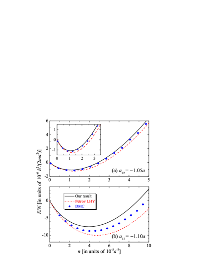
Figure 1: Energy per particle as a function of the density at the interspecies interaction $a_{12}=-1.05a$ (a) and $a_{12}=-1.10a$ (b) and at the equal intraspecies interactions $a_{11}=a_{22}\equiv a$. Our results (black solid line) are compared with Petrov’s MF + LHY prediction (red dashed line) Petrov2015 and the recent DMC data (blue circles) Cikojevic2019 . The inset in (a) highlights the comparison near the equilibrium density.

Equal intraspecies interactions. To see this, let us first focus on the idealized case of $a_{11}=a_{22}$, with which we take $\mu_{1}=\mu_{2}=\mu$ and $\phi_{1c}=\phi_{2c}$, so that $C_{1}=C_{2}=\mu+\Delta>0$ and $B_{1\mathbf{k}}=B_{2\mathbf{k}}=\varepsilon_{\mathbf{k}}+\mu+2\Delta$. The lower and upper Bogoliubov spectra then have the form, $E_{-}(\mathbf{k})=\sqrt{\varepsilon_{\mathbf{k}}(\varepsilon_{\mathbf{k}}+2\mu+4\Delta)}$ and $E_{+}(\mathbf{k})=\sqrt{(\varepsilon_{\mathbf{k}}+2\mu+2\Delta)(\varepsilon_{\mathbf{k}}+2\Delta)}$, respectively. The upper Bogoliubov branch clearly shows an energy gap $E_{\textrm{g}}=2\Delta\sqrt{1+\mu/\Delta}$. Hence, the unstable branch in Petrov’s theory is automatically removed with the introduction of the bosonic pairing. This also implies that we obtain the true ground state of quantum droplets.

We find that at $a_{11}=a_{22}$ the thermodynamic potential becomes ($C=\mu+\Delta$),

$$\varOmega=-\frac{m}{4\pi\hbar^{2}}\left[\frac{C^{2}}{a}+\frac{\Delta^{2}}{a_{12}}\right]+\frac{8m^{3/2}}{15\pi^{2}\hbar^{3}}C^{5/2}\mathcal{G}\left(\frac{\Delta}{C}\right),$$ (10)

where $h(\alpha)\equiv(15/4)\int_{0}^{\infty}dt\sqrt{t}[\sqrt{(t+1)(t+\alpha)}-(t+1/2+\alpha/2)+(1-\alpha)^{2}/(8t)]$ and $\mathcal{G}(\alpha)\equiv(1+\alpha)^{5/2}+h(\alpha)$ slightly differs from $\mathcal{F}(\alpha)$ defined in Eq. (4). As discussed in detail in Supplemental Material SM , for a given chemical potential $\mu$ above a critical value $\mu_{c}<0$, we typically find a minimum in $\varOmega(\Delta)$ located at the pairing parameter $\Delta_{0}\neq 0$. By calculating the density $n=-\partial\varOmega/\partial\mu$, we then obtain the total energy per particle $E/N=\varOmega/n+\mu$ as a function of $n$, which clearly exhibits an absolute minimum anticipated for quantum droplets. At $\mu<\mu_{c}$, $\Delta_{0}$ jumps to zero, indicating a first-order phase transition to a collapsing state for sufficiently small densities CollapseNote .

Numerically, we find $\left|\mu\right|\ll C,\Delta_{0}$, due to the delicate balance in the first term in Eq. (10). As an excellent approximation, we neglect the $\mu$-dependence in the second term and rewrite the regularized LHY thermodynamic potential $\varOmega_{\textrm{LHY}}=[16(2m)^{3/2}/(15\pi^{2}\hbar^{3})]\Delta_{0}^{5/2}$. The dominant $\mu$-dependence in the regularized $\varOmega_{0}$ then leads to $n\simeq m\Delta_{0}/(2\pi\hbar^{2}a)$. Replacing $\Delta_{0}$ by $n$, we obtain,

$$\frac{E}{N}=-\frac{\pi\hbar^{2}}{m}\left(a+\frac{a^{2}}{a_{12}}\right)n+\frac{256\sqrt{\pi}}{15}\frac{\hbar^{2}a^{5/2}}{m}n^{3/2}.$$ (11)

Compared with Eq. (4), it is interesting to see that the approximate LHY term adopted by Petrov is reproduced by our pairing theory and is actually exact at the special case of $a_{11}=a_{12}$. However, the mean-field energy, the first term in Eq. (11), is now changed by a factor of $-a/a_{12}<1$. As a result, the equilibrium density becomes

$$n_{\textrm{eq}}=\frac{25\pi}{16384}\left(1+\frac{a}{a_{12}}\right)^{2}a^{-3}=\frac{a^{2}}{a_{12}^{2}}n_{0},$$ (12)

and is reduced by a factor of $(a/a_{12})^{2}$, with respect to Petrov’s prediction $n_{0}$.

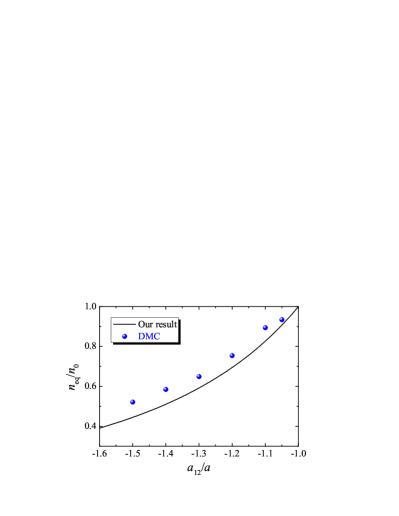
Figure 2: Equilibrium density in units of $n_{0}=[25\pi/16384](1+a_{12}/a)^{2}a^{-3}$ (which is the equilibrium density predicted by Petrov’s theory), as a function of $a_{12}/a$. Our result (black solid line) agrees reasonably well with the DMC data (blue circles).

In Fig. 1, we show the density dependence of the energy per particle given by Eq. (11) (solid line) and Eq. (4) (dashed line) at the interspecies interactions $a_{12}=-1.05a$ (a) and $a_{12}=-1.10a$ (b), and compare them with the benchmark DMC results. We find a good agreement between our result and the DMC data at smaller $\left|a_{12}\right|$ where the gas parameter $na^{3}\sim 10^{-5}$ is small, as exemplified in the inset of Fig. 1(a). At larger $\left|a_{12}\right|$ in (b), our result up-shifts from the DMC data, as the density becomes larger. This is anticipated, as our pairing theory within the Bogoliubov framework only predicts an upper bound for the energy and the higher-order three-body effect beyond LHY should come into a play at density $na^{3}\sim 5\times 10^{-5}$ Wu1959 . In Fig. 2, we report the ratio $n_{\textrm{eq}}/n_{0}$ as a function of $a_{12}/a$. There is a reasonable agreement between our prediction and the DMC data, although our theory becomes increasingly worse at larger $\left|a_{12}/a\right|$ due to the large equilibrium density.

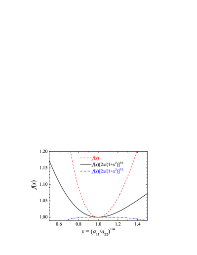
Figure 3: The functions $f(x)$ and $f(x)[2x/(1+x^{2})]^{5/2}$ as a function of $x=(a_{11}/a_{22})^{1/4}$. The latter measures the enhancement of the LHY term in our pairing theory. As shown by the blue dot-dashed line, $f(x)$ can be approximated by $[2x/(1+x^{2})]^{-7/2}$ at the interval $x\subseteq[0.8,1.25]$, within less than $0.1\%$ error in accuracy.

Unequal intraspecies interactions. Let us now consider the realistic situation with unequal intraspecies interactions $a_{11}\neq a_{12}$. It is useful to parametrize the imbalance in the densities by $x=\phi_{2c}/\phi_{1c}=\sqrt{n_{2}/n_{1}}$, so that $C_{1}=\mu_{1}+\Delta x$ and $C_{2}=\mu_{2}+\Delta/x$. In this case, $\left|\mu_{i}\right|\ll C_{i},\Delta_{0}$ near the equilibrium density and it is still an excellent approximation to neglect the $\mu$-dependence in $\varOmega_{\textrm{LHY}}.$ Therefore, we find $\varOmega_{\textrm{LHY}}=[32\sqrt{2}m^{3/2}/(15\pi^{2}\hbar^{3})]\Delta^{5/2}f(x)$, where the detailed expression of $f(x)$ is given in Supplemental Material SM and its value is shown in Fig. 3. In the interval of experimental interest, i.e., $x\subseteq[0.8,1.25]$, to a great accuracy $f(x)\simeq[2x/(1+x^{2})]^{-7/2}.$ On the other hand, the renormalized mean-field thermodynamic potential is given by, $\varOmega_{0}=-[m/(8\pi\hbar^{2})][(\mu_{1}+\Delta x)^{2}/a_{11}+(\mu_{2}+\Delta/x)^{2}/a_{22}+2\Delta^{2}/a_{12}]$, from which we obtain the densities, $n_{1}\simeq xm\Delta_{0}/(4\pi\hbar^{2}a_{11})$ and $n_{2}\simeq x^{-1}m\Delta_{0}/(4\pi\hbar^{2}a_{22})$. Hence,

$$x^{2}=\frac{n_{2}}{n_{1}}=\sqrt{\frac{a_{11}}{a_{22}}},$$ (13)

as predicted by Petrov Petrov2015 . Replacing $\Delta_{0}$ again with the density $n=n_{1}+n_{2}$, we arrive at $E=E_{0}+E_{\textrm{LHY}}$,

$$\frac{E_{0}}{N} = -\frac{\pi\hbar^{2}}{m}\left(a+\frac{a^{2}}{a_{12}}\right)\left[\frac{2x}{1+x^{2}}\right]^{2}n,$$ (14)

$$\frac{E_{\textrm{LHY}}}{N} = \frac{256\sqrt{\pi}}{15}\frac{\hbar^{2}a^{5/2}}{m}\left[\frac{2x}{1+x^{2}}\right]^{5/2}f\left(x\right)n^{3/2}.$$ (15)

Compared with Petrov’s energy at $a_{11}\neq a_{22}$ Petrov2015 , we find that, in addition to the reduction in the mean-field energy as in Eq. (11), the LHY energy is enhanced by a factor of $[2x/(1+x^{2})]^{5/2}f(x)\simeq(1+x^{2})/(2x)$. Therefore, the equilibrium density

$$\frac{n_{\textrm{eq}}}{n_{0}}=\frac{a^{2}}{a_{12}^{2}}\left[\frac{1+x^{2}}{2x}\right]^{5}\frac{1}{f^{2}\left(x\right)}\simeq\frac{a^{2}}{a_{12}^{2}}\left[\frac{2x}{1+x^{2}}\right]^{2}$$ (16)

decreases further at $a_{11}\neq a_{22}$ compared to Petrov’s prediction. In Fig. 4, we present the density dependence of the energy per particle for a ³⁹K Bose-Bose mixture at the magnetic field $B=56.337$G. Our result is compared with the latest DMC data with $N=600$ particles Cikojevic2020 , as well as Petrov’s prediction. The overall agreement with DMC data is reasonable, considering the possible three-body effect beyond LHY at the moderately large density Wu1959 and the finite-size effect at $N=600$ that may slightly down-shift the DMC energy Cikojevic2019 .

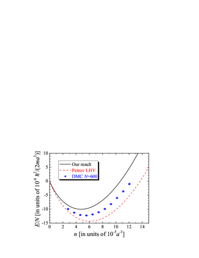
Figure 4: Energy per particle of a ³⁹K-³⁹K Bose mixture at the magnetic field $B=56.337$G, as a function of the total density. Our result (black solid line) is compared with Petrov’s prediction (red dashed line) and the recent DMC data (blue circles) at the number of atoms $N=600$. At this magnetic field, $a_{11}=66.619a_{0}$, $a_{12}=-53.386a_{0}$ and $a_{22}=34.369a_{0}$. We find that $a=(a_{11}a_{22})^{1/2}=47.85a_{0}$ and $x=(a_{11}/a_{22})^{1/4}\simeq 1.180$.

Experimental relevance. Our observation of a reduced equilibrium density in the pairing theory could be related to the smaller-than-expected critical number of atoms found in the first experimental realization of quantum droplets Cabrera2018 . However, for a quantitative comparison, there are several important issues needed to take into account. First, the effective range of interactions of the ³⁹K-³⁹K mixture is fairly large for both intraspecies and interspecies interactions (i.e., $nr_{e}^{3}\sim 0.1-1.0$), which significantly decreases the energy functional Cikojevic2020 . Second, the three-body effect may also play an important role at the gas parameter $na^{3}\sim 10^{-4}$ Wu1959 . At last, an external harmonic trap may turn the experimental setup into an effectively quasi-two-dimensional system Cabrera2018 . These facts will be accounted for in our future studies. Furthermore, in analogy to the conventional BCS superfluid, we anticipate that pair fluctuations give rise to the gapless collective excitations associated with the $U(1)$ symmetry breaking of the pairing field, which can be potentially observed by applying Bragg spectroscopy in future experiments Stenger1999 .

Conclusions. We have developed a consistent theory of quantum droplets and have refined the ground-breaking idea by Petrov that the mean-field collapse can be prevented by quantum fluctuations. Our correct construction of a pairing ground state paves the way to investigate the bosonic BEC-BCS crossover and serves an ideal starting point to explore the finite temperature effect and collective many-body behavior of ultracold, ultradilute quantum droplets.

Appendix A The Bogoliubov theory with bosonic pairing

We use the conventional Bogoliubov theory with pairing to solve a Bose-Bose mixture in the presence of attractive interspecies interaction. The Hamiltonian density of the mixture in real space takes the form,

$$\mathscr{H}\left(\mathbf{x}\right)=\phi_{1}^{\dagger}\left(-\frac{\hbar^{2}\nabla^{2}}{2m}-\mu_{1}\right)\phi_{1}+\phi_{2}^{\dagger}\left(-\frac{\hbar^{2}\nabla^{2}}{2m}-\mu_{2}\right)\phi_{2}+\frac{g_{11}}{2}\phi_{1}^{\dagger}\phi_{1}^{\dagger}\phi_{1}\phi_{1}+\frac{g_{22}}{2}\phi_{2}^{\dagger}\phi_{2}^{\dagger}\phi_{2}\phi_{2}+g_{12}\phi_{1}^{\dagger}\phi_{2}^{\dagger}\phi_{2}\phi_{1},$$ (17)

where $\phi_{i}(\mathbf{x})$ ($i=1,2$) is the annihilation field operator of the $i$-species bosons and $\mu_{i}$ is the chemical potential. The bare interaction strengths $g_{ij}$ are to be replaced by the corresponding $s$-wave scattering length $a_{ij}$, via,

$$\frac{1}{g_{ij}}=\frac{m}{4\pi\hbar^{2}a_{ij}}-\sum_{k}\frac{m}{\hbar^{2}\mathbf{k}^{2}}.$$ (18)

We are interested in calculating the thermodynamic potential $\varOmega$ from the partition function, using the path-integral formalism, $\mathcal{Z}=\int\mathcal{D}[\phi_{1},\phi_{2}]e^{-\mathcal{S}},$ where the action is given by,

$$\mathcal{S}=\int dx\left[\bar{\phi}_{1}\left(x\right)\partial_{\tau}\phi_{1}\left(x\right)+\bar{\phi}_{2}\left(x\right)\partial_{\tau}\phi_{2}\left(x\right)+\mathscr{H}\left(x\right)\right].$$ (19)

Here, we have used the standard notations $x\equiv(\mathbf{x},\tau)$ and $\int dx\equiv\int d\mathbf{x}\int_{0}^{\beta}d\tau$, and $\beta\equiv 1/(k_{B}T)$.

Due to the attractive interspecies interaction ($g_{12}<0$), we may anticipate the pairing between different species. Therefore, we use the Hubbard–Stratonovich (HS) transformation to decouple the last term in the Hamiltonian density,

$$e^{-g_{12}\int dx\bar{\phi}_{1}\bar{\phi}_{2}\phi_{2}\phi_{1}}=\int\mathcal{D}\left[\Delta\left(x\right)\right]\exp\left\{\int dx\left[\frac{\left|\Delta\left(x\right)\right|^{2}}{g_{12}}+\left(\bar{\Delta}\phi_{2}\phi_{1}+\bar{\phi}_{1}\bar{\phi}_{2}\Delta\right)\right]\right\}.$$ (20)

The action then takes the form,

$$\mathcal{S}=\int dx\left\{-\frac{\left|\Delta\left(x\right)\right|^{2}}{g_{12}}-\left(\bar{\Delta}\phi_{2}\phi_{1}+\bar{\phi}_{1}\bar{\phi}_{2}\Delta\right)+\sum_{i=1,2}\left[\bar{\phi}_{i}\left(\partial_{\tau}-\frac{\hbar^{2}\nabla^{2}}{2m}-\mu_{i}\right)\phi_{i}+\frac{g_{ii}}{2}\bar{\phi}_{i}\bar{\phi}_{i}\phi_{i}\phi_{i}\right]\right\}.$$ (21)

For the pairing field $\Delta(x)$, it suffices to take a uniform saddle-point solution $\Delta(x)=\Delta>0$. At the same level of approximation, we assume the bosons condensate into the zero-momentum states, i.e.,

$$\phi_{i}\left(x\right) = \phi_{ic}+\delta\phi_{i}\left(x\right),$$ (22)

with a real positive $\phi_{ic}>0$, and we approximate the intraspecies interaction terms (i.e., within the Bogoliubov approximation),

$$\frac{g_{ii}}{2}\bar{\phi}_{i}\bar{\phi}_{i}\phi_{i}\phi_{i}\simeq\frac{g_{ii}}{2}\phi_{ic}^{4}+2g_{ii}\phi_{ic}^{2}\delta\bar{\phi}_{i}\delta\phi_{i}+\frac{g_{ii}\phi_{ic}^{2}}{2}\left(\delta\bar{\phi}_{i}\delta\bar{\phi}_{i}+\delta\phi_{i}\delta\phi_{i}\right).$$ (23)

As a result, we find that $\mathcal{S}=\mathcal{S}_{0}+\mathcal{S}_{B}$, where,

$$S_{0} = \beta\mathcal{V}\left[\sum_{i=1,2}\left(-\mu_{i}\phi_{ic}^{2}+\frac{g_{ii}}{2}\phi_{ic}^{4}\right)-\frac{\Delta^{2}}{g_{12}}-2\Delta\phi_{1c}\phi_{2c}\right],$$ (24)

$$\mathcal{S}_{B} = \int dx\left\{\sum_{i=1,2}\left[\delta\bar{\phi}_{i}\left(\partial_{\tau}-\frac{\hbar^{2}\nabla^{2}}{2m}-\mu_{i}+2g_{ii}\phi_{ic}^{2}\right)\delta\phi_{i}+\frac{g_{ii}\phi_{ic}^{2}}{2}\left(\delta\bar{\phi}_{i}\delta\bar{\phi}_{i}+\delta\phi_{i}\delta\phi_{i}\right)\right]-\Delta\left(\delta\phi_{2}\delta\phi_{1}+\delta\bar{\phi}_{1}\delta\bar{\phi}_{2}\right)\right\}.$$ (25)

By introducing the notations $C_{i}=g_{ii}\phi_{ic}^{2}$ and a Nambu spinor $\Phi(x)=[\delta\phi_{1}(x),\delta\bar{\phi}_{1}(x),\delta\phi_{2}(x),\delta\bar{\phi}_{2}(x)]^{T}$, we may rewrite $\mathcal{S}_{B}$ into a compact form,

$$\mathcal{S}_{B}=\int dxdx^{\prime}\bar{\Phi}\left(x\right)\left[-\mathscr{D}^{-1}\left(x,x^{\prime}\right)\right]\Phi\left(x^{\prime}\right),$$ (26)

where the inverse Green function of bosons is given by,

$$-\mathscr{D}^{-1}=\left[\begin{array}[]{cccc}\partial_{\tau}-\frac{\hbar^{2}\nabla^{2}}{2m}-\mu_{1}+2C_{1}&C_{1}&0&-\Delta\\ C_{1}&-\partial_{\tau}-\frac{\hbar^{2}\nabla^{2}}{2m}-\mu_{1}+2C_{1}&-\Delta&0\\ 0&-\Delta&\partial_{\tau}-\frac{\hbar^{2}\nabla^{2}}{2m}-\mu_{2}+2C_{2}&C_{2}\\ -\Delta&0&C_{2}&-\partial_{\tau}-\frac{\hbar^{2}\nabla^{2}}{2m}-\mu_{2}+2C_{2}\end{array}\right].$$ (27)

We do not explicitly show the delta function $\delta\left(x-x^{\prime}\right)$ in $\mathscr{D}^{-1}(x,x^{\prime})$. By taking a Fourier transform, then, in momentum space the bosonic Green function takes the form (after transforming $\partial_{\tau}\rightarrow-i\omega_{m}$ and taking the bosonic Matasubara frequencies, $i\omega_{m}\rightarrow\omega$),

$$\mathscr{D}^{-1}\left(\mathbf{k},\omega\right)=\left[\begin{array}[]{cccc}\omega-B_{1\mathbf{k}}&-C_{1}&0&\Delta\\ -C_{1}&-\omega-B_{1\mathbf{k}}&\Delta&0\\ 0&\Delta&\omega-B_{2\mathbf{k}}&-C_{2}\\ \Delta&0&-C_{2}&-\omega-B_{2\mathbf{k}}\end{array}\right],$$ (28)

where we have defined,

$$B_{i\mathbf{k}}\equiv\frac{\hbar^{2}\mathbf{k}^{2}}{2m}-\mu_{i}+2C_{i}=\varepsilon_{\mathbf{k}}-\mu_{i}+2C_{i}.$$ (29)

By solving the poles of the bosonic Green function, i.e., $\det[\mathscr{D}^{-1}(\mathbf{k},\omega\rightarrow E(\mathbf{k}))]=0$, or more explicitly,

$$\omega^{4}-\omega^{2}\left[\left(B_{1\mathbf{k}}^{2}-C_{1}^{2}\right)+\left(B_{2\mathbf{k}}^{2}-C_{2}^{2}\right)-2\Delta^{2}\right]+\left[\left(B_{1\mathbf{k}}^{2}-C_{1}^{2}\right)\left(B_{2\mathbf{k}}^{2}-C_{2}^{2}\right)-2\left(B_{1\mathbf{k}}B_{2\mathbf{k}}+C_{1}C_{2}\right)\Delta^{2}+\Delta^{4}\right]=0,$$ (30)

we obtain the two Bogoliubov spectra,

$$E_{\pm}^{2}\left(\mathbf{k}\right)=\left[\mathcal{A}_{+}\left(\mathbf{k}\right)-\Delta^{2}\right]\pm\sqrt{\mathcal{A}_{-}^{2}\left(\mathbf{k}\right)+\Delta^{2}\left[\left(C_{1}+C_{2}\right)^{2}-\left(B_{1\mathbf{k}}-B_{2\mathbf{k}}\right)^{2}\right]},$$ (31)

with

$$\mathcal{A}_{\pm}\left(\mathbf{k}\right)=\frac{\left(B_{1\mathbf{k}}^{2}-C_{1}^{2}\right)\pm\left(B_{2\mathbf{k}}^{2}-C_{2}^{2}\right)}{2}.$$ (32)

A.1 Thermodynamic potential from the condensate

From the condensate contribution $\mathcal{S}_{0}$, we write down the corresponding thermodynamic potential at the tree level,

$$\varOmega_{0}=-\frac{\Delta^{2}}{g_{12}}-2\Delta\phi_{1c}\phi_{2c}+\left(-\mu_{1}\phi_{1c}^{2}+\frac{g_{11}}{2}\phi_{1c}^{4}\right)+\left(-\mu_{2}\phi_{2c}^{2}+\frac{g_{22}}{2}\phi_{2c}^{4}\right).$$ (33)

By taking the derivative of $\varOmega_{0}$ with respect to $\phi_{1c}$ and $\phi_{2c}$, we obtain,

$$-\mu_{1}\phi_{1c}+g_{11}\phi_{1c}^{3}-\Delta\phi_{2c} = 0,$$ (34)

$$-\mu_{2}\phi_{2c}+g_{22}\phi_{2c}^{3}-\Delta\phi_{1c} = 0.$$ (35)

Therefore, we have,

$$-\mu_{1}+C_{1}=B_{1\mathbf{k}=0}-C_{1} = \Delta\frac{\phi_{2c}}{\phi_{1c}},$$ (36)

$$-\mu_{2}+C_{2}=B_{2\mathbf{k}=0}-C_{2} = \Delta\frac{\phi_{1c}}{\phi_{2c}}.$$ (37)

It is easy to see that,

$$\left(B_{1\mathbf{k}=0}-C_{1}\right)\left(B_{2\mathbf{k}=0}-C_{2}\right)=\Delta^{2}.$$ (38)

As the last term in Eq. (30) can be rewritten as,

$$\left[\left(B_{1\mathbf{k}}-C_{1}\right)\left(B_{2\mathbf{k}}-C_{2}\right)-\Delta^{2}\right]\left[\left(B_{1\mathbf{k}}+C_{1}\right)\left(B_{2\mathbf{k}}+C_{2}\right)-\Delta^{2}\right],$$ (39)

the term is zero at $\mathbf{k}=0$. Thus, we confirm that at least one of the two Bogoliubov spectra is gapless. This is anticipated from the $U(1)$ symmetry breaking of the system. On the other hand, it is also straightforward to confirm that,

$$\varOmega_{0}=-\frac{\Delta^{2}}{g_{12}}-\frac{C_{1}^{2}}{2g_{11}}-\frac{C_{2}^{2}}{2g_{22}}=-\frac{m}{4\pi\hbar^{2}}\left[\frac{\Delta^{2}}{a_{12}}+\frac{C_{1}^{2}}{2a_{11}}+\frac{C_{2}^{2}}{2a_{22}}\right]+\frac{1}{2}\sum_{\mathbf{k}}\frac{C_{1}^{2}+C_{2}^{2}+2\Delta^{2}}{\hbar^{2}\mathbf{k}^{2}/m},$$ (40)

where in the last step, we have replaced the bare interaction strengths by using the $s$-wave scattering lengths.

A.2 LHY thermodynamic potential

The LHY thermodynamic potential at the one-loop level can obtained from $\mathcal{S}_{B}$ Salasnich2016 ; Hu2020 ,

$$\varOmega_{\textrm{LHY}}=\frac{k_{B}T}{2}\sum_{\mathbf{q},i\omega_{m}}\ln\det\left[\mathscr{-D}^{-1}\left(\mathbf{q},i\omega_{m}\right)\right]e^{i\omega_{m}0^{+}}=\frac{1}{2}\sum_{\mathbf{k}}\left[E_{+}\left(\mathbf{k}\right)+E_{-}\left(\mathbf{k}\right)-B_{1\mathbf{k}}-B_{2\mathbf{k}}\right].$$ (41)

By putting together $\varOmega_{0}$ and $\varOmega_{\textrm{LHY}},$we obtain the thermodynamic potential within the Bogoliubov approximation,

$$\varOmega=-\frac{m}{4\pi\hbar^{2}}\left[\frac{\Delta^{2}}{a_{12}}+\frac{C_{1}^{2}}{2a_{11}}+\frac{C_{2}^{2}}{2a_{22}}\right]+\frac{1}{2}\sum_{\mathbf{k}}\left[E_{+}\left(\mathbf{k}\right)+E_{-}\left(\mathbf{k}\right)-B_{1\mathbf{k}}-B_{2\mathbf{k}}+\frac{C_{1}^{2}+C_{2}^{2}+2\Delta^{2}}{\hbar^{2}\mathbf{k}^{2}/m}\right].$$ (42)

Appendix B Equal intraspecies interactions

In this case, $C_{1}=C_{2}=C=\mu+\Delta>0$ and $B_{1\mathbf{k}}=B_{2\mathbf{k}}=\varepsilon_{\mathbf{k}}+\mu+2\Delta$, and the thermodynamic potential is given by,

$$\varOmega=-\frac{m}{4\pi\hbar^{2}}\left[\frac{C^{2}}{a}+\frac{\Delta^{2}}{a_{12}}\right]+\frac{1}{2}\sum_{\mathbf{k}}\left[E_{+}\left(\mathbf{k}\right)+E_{-}\left(\mathbf{k}\right)-2\left(\varepsilon_{\mathbf{k}}+C+\Delta\right)+\frac{2\left(C^{2}+\Delta^{2}\right)}{\hbar^{2}\mathbf{k}^{2}/m}\right],$$ (43)

where $\varepsilon_{\mathbf{k}}\equiv\hbar^{2}k^{2}/(2m)$ and two Bogoliubov spectra are,

$$E_{-}(\mathbf{k}) = \sqrt{\varepsilon_{\mathbf{k}}\left(\varepsilon_{\mathbf{k}}+2C+2\Delta\right)},$$ (44)

$$E_{+}(\mathbf{k}) = \sqrt{\left(\varepsilon_{\mathbf{k}}+2C\right)\left(\varepsilon_{\mathbf{k}}+2\Delta\right)}.$$ (45)

The integral can be separated into two parts $\mathcal{I}_{+}$ and $\mathcal{I}_{-}$, where

$$\mathcal{I}_{\pm}=\frac{1}{2}\sum_{\mathbf{k}}\left[E_{\pm}\left(\mathbf{k}\right)-\left(\varepsilon_{\mathbf{k}}+C+\Delta\right)+\frac{\left(C\pm\Delta\right)^{2}}{\hbar^{2}\mathbf{k}^{2}/m}\right].$$ (46)

By introducing a new variable $t\equiv[\hbar^{2}k^{2}/(2m)]/[2(C+\Delta)]$, it is easy to see that,

$$\mathcal{I}_{-}=\frac{1}{8\pi^{2}}\left(\frac{2m}{\hbar^{2}}\right)^{3/2}\left[2\left(C+\Delta\right)\right]^{5/2}\int_{0}^{\infty}dt\sqrt{t}\left[\sqrt{t\left(t+1\right)}-\left(t+\frac{1}{2}\right)+\frac{1}{8t}\right]=\frac{8m^{3/2}}{15\pi^{2}\hbar^{3}}C^{5/2}\left(1+\frac{\Delta}{C}\right)^{5/2}.$$ (47)

To calculate $\mathcal{I}_{+}$, we instead introduce $t\equiv[\hbar^{2}k^{2}/(2m)]/(2C)$ and $\alpha\equiv\Delta/C$, which leads to,

$$\mathcal{I}_{+}=\frac{1}{8\pi^{2}}\left(\frac{2m}{\hbar^{2}}\right)^{3/2}\left[2C\right]^{5/2}\int_{0}^{\infty}dt\sqrt{t}\left[\sqrt{\left(t+1\right)\left(t+\alpha\right)}-\left(t+\frac{1+\alpha}{2}\right)+\frac{\left(1-\alpha\right)^{2}}{8t}\right]\equiv\frac{8m^{3/2}}{15\pi^{2}\hbar^{3}}C^{5/2}h\left(\alpha\right).$$ (48)

By adding up $\mathcal{I}_{+}$ and $\mathcal{I}_{-}$, we obtain the LHY term,

$$\varOmega_{\textrm{LHY}}=\mathcal{I}_{+}+\mathcal{I}_{-}=\frac{8m^{3/2}}{15\pi^{2}\hbar^{3}}\left(\mu+\Delta\right)^{5/2}\mathcal{G}\left(\frac{\Delta}{\mu+\Delta}\right),$$ (49)

where $\mathcal{G}(\alpha)\equiv(1+\alpha)^{5/2}+h\left(\alpha\right)$. It is easy to obtain that $h(0)=1$, $h(1)=0$, $h^{\prime}(1)=0$ and $h^{\prime\prime}(1)=15\pi/16$. Compared with the function $\mathcal{F}(\alpha)\equiv(1+\alpha)^{5/2}+(1-\alpha)^{5/2}$ for the LHY energy in the Bogoliubov theory of a Bose-Bose mixture, we find the role of $(1-\alpha)^{5/2}$, which is not well-defined for $\alpha>1$, is now replaced by a new function $h(\alpha)$. In Fig. 5, we show the function $h(\alpha)$. It is larger than $(1-\alpha)^{5/2}$ in the interval $\alpha\subseteq[0,1]$.

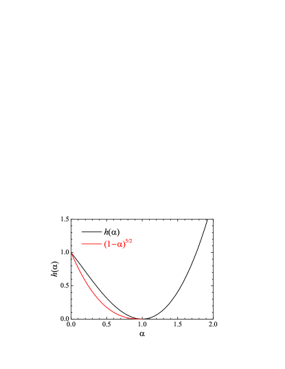
Figure 5: The function $h(\alpha)$ and its comparison to $(1-\alpha)^{5/2}$.

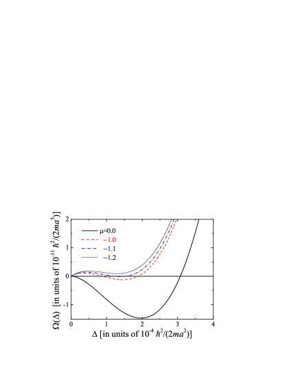
Figure 6: Thermodynamic potential $\varOmega$, in units of $10^{-11}\hbar^{2}/(2ma^{5})$, as a function of the pairing parameter $\Delta$, at different chemical potentials $\mu=0$ (black solid line), $-1.0$ (red dashed line), $-1.1$ (blue dot-dashed line), and $-1.2$ (black dotted line), and at $a_{12}=-1.05a$. $\Delta$ and $\mu$ are measured in units of $10^{-4}\hbar^{2}/(2ma^{2})$ and $10^{-6}\hbar^{2}/(2ma^{2})$, respectively. The critical chemical potential is about $\mu_{c}\simeq-1.1\times 10^{-6}\hbar^{2}/(2ma^{2})$.

Let us now consider the total thermodynamic potential,

$$\varOmega=-\frac{m}{4\pi\hbar^{2}}\left[\frac{\left(\mu+\Delta\right)^{2}}{a}+\frac{\Delta^{2}}{a_{12}}\right]+\frac{8m^{3/2}}{15\pi^{2}\hbar^{3}}\left(\mu+\Delta\right)^{5/2}\mathcal{G}\left(\frac{\Delta}{\mu+\Delta}\right).$$ (50)

For a given chemical potential $\mu$, we need to the minimize $\varOmega$ to determine the pairing order parameter $\Delta_{0}$, and then calculate the total density of the system, i.e., $n=-\partial\varOmega/\partial\mu$. In Fig. 6, we show the thermodynamic potential $\varOmega$ as a function of $\Delta$, at four different chemical potentials $\mu=0$, $-1.0$, $-1.1$ , and $-1.2$, which is measured in units of $10^{-4}\hbar^{2}/(2ma^{2})$, and at $a_{12}=-1.05a$. For the chemical potential above a critical value, i.e., $\mu_{c}\simeq-1.1\times 10^{-4}\hbar^{2}/(2ma^{2})$, we typically find a global minimum in the thermodynamic potential at $\Delta_{0}\neq 0$. For $\mu<\mu_{c}$, it turns into a local minimum and the thermodynamic potential takes the global minimum at $\Delta_{0}=0$. The change of the global minimum position $\Delta_{0}$ is not continuous at $\mu=\mu_{c}$, indicating a first-order quantum phase transition into a collapsing phase.

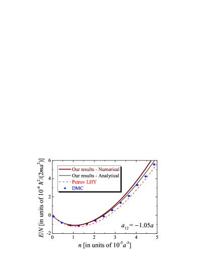
Figure 7: Energy per particle as a function of the density at the interspecies interaction $a_{12}=-1.05a$ and at the equal intraspecies interactions $a_{11}=a_{22}\equiv a$. Our analytic result (black solid line) is compared with Petrov’s MF + LHY prediction (red dashed line) Petrov2015 and the recent DMC data (blue circles) Cikojevic2019 . Our full numerical result is shown by the brown solid thick line.

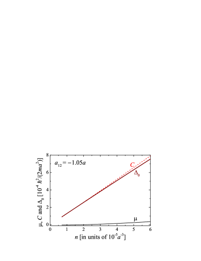
Figure 8: Chemical potential $\mu$, the parameter $C$ and the pairing gap $\Delta_{0}$, in units of $10^{-4}\hbar^{2}/(2ma^{2})$, as a function of the total density $n$ (in units of $10^{-5}a^{-3}$) at $a_{12}=-1.05a$.

For nonzero $\Delta_{0}\neq 0$, we obtain $\varOmega(\mu,\Delta_{0})$ and calculate $n=-\partial\varOmega(\mu,\Delta_{0})/\partial\mu$. Hence, we numerically obtain the total energy $E=\varOmega+\mu n$. This energy is shown in Fig. 7 by using a brown thick solid line, as a function of the total density. It turns out that numerically the chemical potential is much smaller than either the parameter $C$ or the pairing gap $\Delta$ , as can be clearly seen from Fig. 8. This is easy to understand from the $\Delta$-dependence in $\varOmega_{0}$ and $\varOmega_{\textrm{LHY}}.$ We note that two terms in $\varOmega_{0}$ are large and have opposite sign. Each of them (i.e., absolute value) is much larger than $\varOmega_{\textrm{LHY}}$. Therefore, when we minimize $\varOmega$ with respect to $\Delta$, we only need to minimize $\Omega_{0}$. This leads to the condition,

$$\frac{\mu+\Delta}{a}+\frac{\Delta}{a_{12}}\simeq 0.$$ (51)

Therefore, we find that,

$$\mu\simeq-\left(1+\frac{a}{a_{12}}\right)\Delta\ll\Delta,C$$ (52)

as a result of $a_{12}\sim-a$.

Due to the smallness of $\left|\mu\right|$, it is reasonable to neglect the $\mu$-dependence in $\varOmega_{\textrm{LHY}}$ and the term $\mu^{2}$ in $\varOmega_{0}$. Therefore, we obtain,

$$\varOmega\simeq-\frac{m}{4\pi\hbar^{2}}\left[\frac{2\mu\Delta}{a}+\frac{\Delta^{2}}{a}+\frac{\Delta^{2}}{a_{12}}\right]+\frac{32\sqrt{2}m^{3/2}}{15\pi^{2}\hbar^{3}}\Delta^{5/2}.$$ (53)

By taking the derivative with respect to $\mu$, we obtain

$$n=-\frac{\partial\varOmega}{\partial\mu}\simeq\frac{m}{2\pi\hbar^{2}a}\Delta_{0},$$ (54)

where we determine $\varOmega$ at the saddle point $\Delta=\Delta_{0}$. Replacing the pairing parameter $\Delta_{0}$ by the density $n$, we finally arrive at (the volume $\mathcal{V}=1$),

$$\frac{E}{N}=\frac{\varOmega}{n}+\mu=-\frac{\pi\hbar^{2}}{m}\left(a+\frac{a^{2}}{a_{12}}\right)n+\frac{256\sqrt{\pi}}{15}\frac{\hbar^{2}a^{5/2}}{m}n^{3/2}.$$ (55)

In Fig. 7, this analytic result is shown by the black solid line. We find an excellent agreement near the equilibrium density between the analytic result and the full numerical result for the energy per particle. However, for the density $n>3\times 10^{-5}a^{-3}$, the difference starts to become visible. This is not a serious problem, as our perturbative treatment within in the Bogoliubov theory is anticipated to become worse at similar densities. Thus, it is useless to quantify the difference between the analytic and numerical results.

Appendix C Unequal intraspecies interactions

Let us now consider the unequal intraspecies interactions, with which there could be an imbalanced in the species population, given by $x=\phi_{2c}/\phi_{1c}=\sqrt{n_{2}/n_{1}}$. Taking the small chemical potential limit as in the case of equal intraspecies interactions, i.e., $\mu_{1}=\mu_{2}=0$ in $\varOmega_{\textrm{LHY}}$, we find that,

$$C_{1} = x\Delta,$$ (56)

$$C_{2} = x^{-1}\Delta,$$ (57)

$$B_{1\mathbf{k}} = \frac{\hbar^{2}\mathbf{k}^{2}}{2m}+2x\Delta,$$ (58)

$$B_{2\mathbf{k}} = \frac{\hbar^{2}\mathbf{k}^{2}}{2m}+2x^{-1}\Delta.$$ (59)

By introducing the variable $t=[\hbar^{2}k^{2}/(2m)]/(2\Delta)$, we can write $\varOmega_{\textrm{LHY}}$ into the form,

$$\varOmega_{\textrm{LHY}}=\frac{32\sqrt{2}m^{3/2}}{15\pi^{2}\hbar^{3}}\Delta^{5/2}f\left(x\right),$$ (60)

where the function is defined by,

$$f\left(x\right)=\frac{15\sqrt{2}}{32}\int_{0}^{\infty}dt\sqrt{t}\left[\tilde{E}_{+}\left(t\right)+\tilde{E}_{-}\left(t\right)-\left(2t+x+x^{-1}\right)+\frac{\left(x+x^{-1}\right)^{2}}{8t}\right],$$ (61)

with

$$\tilde{E}_{\pm}^{2}\left(t\right)=\frac{\left(\tilde{B}_{1t}^{2}-\tilde{C}_{1}^{2}\right)+\left(\tilde{B}_{2t}^{2}-\tilde{C}_{2}^{2}\right)^{2}}{2}-\frac{1}{4}\pm\frac{1}{2}\sqrt{\left[\left(\tilde{B}_{1t}^{2}-\tilde{C}_{1}^{2}\right)-\left(\tilde{B}_{2t}^{2}-\tilde{C}_{2}^{2}\right)^{2}\right]^{2}+\left(\tilde{C}_{1}+\tilde{C}_{2}\right)^{2}-\left(\tilde{B}_{1t}-\tilde{B}_{2t}\right)^{2}}.$$ (62)

Here, we have introduced the notations: $\tilde{C}_{1}=x/2$, $\tilde{C}_{2}=x^{-1}/2$, $\tilde{B}_{1t}=t+x$ and $\tilde{B}_{2t}=t+x^{-1}$.

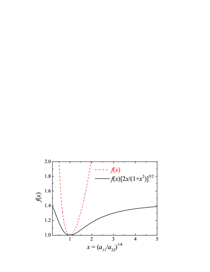
Figure 9: The function $f(x)$ and the enhancement factor $f(x)[2x/(1+x^{2})]^{5/2}$ as a function of $x=(a_{11}/a_{22})^{1/4}$. We note that, both functions are symmetric with respect to the point $x=1$, i.e., $f(x)=f(x^{-1}).$

By adding $\varOmega_{0}$, we obtain at the unequal intraspecies interactions,

$$\varOmega\simeq-\frac{m}{8\pi\hbar^{2}}\left[\frac{\mu_{1}x\Delta}{a_{11}}+\frac{\mu_{2}x^{-1}\Delta}{a_{22}}+\frac{x^{2}\Delta^{2}}{a_{11}}+\frac{x^{-2}\Delta^{2}}{a_{22}}+\frac{2\Delta^{2}}{a_{12}}\right]+\frac{32\sqrt{2}m^{3/2}}{15\pi^{2}\hbar^{3}}\Delta^{5/2}f\left(x\right).$$ (63)

Taking the saddle point $\Delta=\Delta_{0}$ and the derivative of $\varOmega(\Delta_{0})$with respect to $\mu_{1}$ and $\mu_{2}$, we find that,

$$n_{1} \simeq \frac{xm\Delta_{0}}{4\pi\hbar^{2}a_{11}},$$ (64)

$$n_{2} \simeq \frac{x^{-1}m\Delta_{0}}{4\pi\hbar^{2}a_{22}}.$$ (65)

By dividing these two expressions with each other, we find that

$$x^{2}=\frac{n_{2}}{n_{1}}=\sqrt{\frac{a_{11}}{a_{22}}}.$$ (66)

This identity has also obtained in Petrov’s theory, although a quite different derivation (i.e., starting from the mean-field energy, which is different from ours) is demonstrated. The coincidence is interesting. We can replace the pairing parameter $\Delta_{0}$ by the density, i.e.,

$$\Delta_{0}=\frac{4\pi\hbar^{2}\sqrt{a_{11}a_{22}}}{m}\left(n_{1}n_{2}\right)^{/12}=\frac{4\pi\hbar^{2}a}{m}\left(n_{1}n_{2}\right)^{/12}.$$ (67)

By calculating the total energy $E=\varOmega+\mu_{1}n_{1}+\mu_{2}n_{2}$, we obtain,

$$\frac{E}{N}=-\frac{\pi\hbar^{2}}{m}\left(a+\frac{a^{2}}{a_{12}}\right)\left[\frac{2x}{1+x^{2}}\right]^{2}n+\frac{256\sqrt{\pi}}{15}\frac{\hbar^{2}a^{5/2}}{m}\left[\frac{2x}{1+x^{2}}\right]^{5/2}f\left(x\right)n^{3/2}.$$ (68)

This energy is to be compared with Petrov’s prediction Petrov2015 ,

$$\frac{E_{\textrm{Petrov}}}{N}=\frac{\pi\hbar^{2}}{m}\left(a+a_{12}\right)\left[\frac{2x}{1+x^{2}}\right]^{2}n+\frac{256\sqrt{\pi}}{15}\frac{\hbar^{2}a^{5/2}}{m}n^{3/2}.$$ (69)

We emphasize that in our pairing theory, the LHY energy term is enhanced by a factor of

$$\eta\left(x\right)=\left[\frac{2x}{1+x^{2}}\right]^{5/2}f\left(x\right),$$ (70)

which could be very significant for a large imbalance in intraspecies interactions. For example, if $x=2$ (or $x=0.5$) at $a_{11}=16a_{22}$ (or $a_{11}=a_{22}/16$), the enhancement factor can be around $\eta\simeq 1.2$ and hence decrease the equilibrium density by a factor of $\eta^{2}\simeq 1.4$. In the current experiments of a ³⁹K Bose-Bose mixture, the ratio of $a_{11}/a_{22}$ is about $2$ and then $x\simeq 1.2$. Therefore, the enhancement in the LHY energy is just a few percent.

References

(1)D. S. Petrov, Liquid beyond the van der Waals
paradigm, Nat. Phys. 14, 211 (2018).
(3)Y. Kartashov, G. Astrakharchik, B. Malomed,
and L. Torner, Frontiers in multidimensional self-trapping of nonlinear
fields and matter, Nat. Rev. Phys. 1, 185 (2019).
(4)For a recent review, see, for example, F. Böttcher,
J.-N. Schmidt, J. Hertkorn, K. S. H. Ng, S. D. Graham, M. Guo, T.
Langen, and T. Pfau, New states of matter with fine-tuned interactions:
quantum droplets and dipolar supersolids, arXiv:2007.06391 (2020).
(5)I. Ferrier-Barbut, H. Kadau, M. Schmitt,
M. Wenzel, and T. Pfau, Observation of Quantum Droplets in a Strongly
Dipolar Bose Gas, Phys. Rev. Lett. 116, 215301 (2016).
(6)M. Schmitt, M. Wenzel, F. Böttcher, I. Ferrier-Barbut,
and T. Pfau, Self-bound droplets of a dilute magnetic quantum liquid,
Nature (London) 539, 259 (2016).
(7)L. Chomaz, S. Baier, D. Petter, M. J. Mark, F.
Wächtler, L. Santos, and F. Ferlaino, Quantum-Fluctuation-Driven Crossover
from a Dilute Bose-Einstein Condensate to a Macrodroplet in a Dipolar
Quantum Fluid, Phys. Rev. X 6, 041039 (2016).
(8)C. Cabrera, L. Tanzi, J. Sanz, B. Naylor, P.
Thomas, P. Cheiney, and L. Tarruell, Quantum liquid droplets in a
mixture of Bose-Einstein condensates, Science 359, 301 (2018).
(9)G. Semeghini, G. Ferioli, L. Masi, C. Mazzinghi,
L. Wolswijk, F. Minardi, M. Modugno, G. Modugno, M. Inguscio, and
M. Fattori, Self-Bound Quantum Droplets of Atomic Mixtures in Free
Space, Phys. Rev. Lett. 120, 235301 (2018).
(10)F. Böttcher, M. Wenzel, J.-N. Schmidt, M. Guo,
T. Langen, I. Ferrier-Barbut, T. Pfau, R. Bombín, J. Sánchez-Baena,
J. Boronat, and F. Mazzanti, Dilute dipolar quantum droplets beyond
the extended Gross-Pitaevskii equation, Phys. Rev. Research 1,
033088 (2019).
(11)D. S. Petrov, Quantum Mechanical Stabilization
of a Collapsing Bose-Bose Mixture, Phys. Rev. Lett. 115,
155302 (2015).
(12)D. M. Larsen, Binary mixtures of dilute Bose
gases with repulsive interactions at low temperature, Ann. Phys. (N.Y.)
24, 89 (1963).
(13)T. D. Lee, K. Huang, and C. N. Yang, Eigenvalues
and Eigenfunctions of a Bose System of Hard Spheres and Its Low-Temperature
Properties, Phys. Rev. 106, 1135 (1957).
(14)P. Cheiney, C. R. Cabrera, J. Sanz, B. Naylor,
L. Tanzi, and L. Tarruell, Bright Soliton to Quantum Droplet Transition
in a Mixture of Bose-Einstein Condensates, Phys. Rev. Lett. 120,
135301 (2018).
(15)G. Ferioli, G. Semeghini, L. Masi, G. Giusti,
G. Modugno, M. Inguscio, A. Gallemi, A. Recati, and M. Fattori, Collisions
of Self-Bound Quantum Droplets, Phys. Rev. Lett. 122, 090401
(2019).
(16)C. D’Errico, A. Burchianti, M.
Prevedelli, L. Salasnich, F. Ancilotto, M. Modugno, F. Minardi, and
C. Fort, Observation of quantum droplets in a heteronuclear bosonic
mixture, Phys. Rev. Research 1, 033155 (2019).
(17)D. S. Petrov and G. E. Astrakharchik, Ultradilute
Low-Dimensional Liquids, Phys. Rev. Lett. 117, 100401 (2016).
(18)A. Cappellaro, T. Macrì, G. F. Bertacco,
and L. Salasnich, Equation of state and self-bound droplet in Rabi-coupled
Bose mixtures, Sci. Rep. 7, 13358 (2017).
(19)Y. Li, Z. Luo, Y. Liu, Z. Chen, C. Huang, S. Fu,
H. Tan, and B. A. Malomed, Two-dimensional solitons and quantum droplets
supported by competing self- and cross-interactions in spin-orbit-coupled
condensates, New J. Phys. 19, 113043 (2017).
(20)X. Cui, Spin-orbit-coupling-induced quantum droplet
in ultracold Bose-Fermi mixtures, Phys. Rev. A 98, 023630
(2018).
(21)N. B. Jørgensen, G. M. Bruun, and J. J. Arlt,
Dilute Fluid Governed by Quantum Fluctuations, Phys. Rev. Lett. 121,
173403 (2018).
(22)T. Shi, J. Pan, and S. Yi, Trapped Bose-Einstein
Condensates with Attractive -wave Interaction, arXiv:1909.02432
(2019).
(23)Y. Wang, L. Guo, S. Yi, and T. Shi, Theory for
Self-Bound States of Dipolar Bose-Einstein Condensates, arXiv:2002.11298
(2020).
(24)V. Cikojević, L. Vranješ Markic, G. E.
Astrakharchik, and J. Boronat, Universality in ultradilute liquid
Bose-Bose mixtures, Phys. Rev. A 99, 023618 (2019).
(25)L. Parisi, G. E. Astrakharchik,
and S. Giorgini, Liquid State of One-Dimensional Bose Mixtures: A
Quantum Monte Carlo Study, Phys. Rev. Lett. 122, 105302 (2019).
(26)V. Cikojević, L. Vranješ Markić, and
J. Boronat, Finite-range effects in ultradilute quantum drops, New
J. Phys. 22, 053045 (2020).
(27)J. Bardeen, L. N. Cooper, and J. R. Schrieffer,
Microscopic Theory of Superconductivity, Phys. Rev. 106,
162 (1957).
(28)S. Stringari and J. Treiner, Surface properties
of liquid 3He and 4He: A density-functional approach,
Phys. Rev. B 36, 8369 (1987).
(29)F. Dalfovo, A. Lastri, L. Pricaupenko, S. Stringari,
and J. Treiner, Structural and dynamical properties of superfluid
helium: A density-functional approach, Phys. Rev. B 52, 1193
(1995).
(30)F. Laimer, L. Kranabetter, L. Tiefenthaler, S.
Albertini, F. Zappa, A. M. Ellis, M. Gatchell, and P. Scheier, Highly
Charged Droplets of Superfluid Helium, Phys. Rev. Lett. 123,
165301 (2019).
(31)A. E. Almand-Hunter, H. Li, S. T. Cundiff,
M. Mootz, M. Kira, and S. W. Koch, Quantum droplets of electrons and
holes, Nature (London) 506, 471 (2014).
(32)T. B. Arp, D. Pleskot, V. Aji, and N. M. Gabor,
Electron–hole liquid in a van der Waals heterostructure photocell
at room temperature, Nat. Photon. 13, 245 (2019).
(33)H. Hu, X.-J. Liu, and P. D. Drummond, Equation of
state of a superfluid Fermi gas in the BCS-BEC crossover, Europhys.
Lett. 74, 574 (2006).
(34)H. Hu, P. D. Drummond, and X.-J. Liu, Universal thermodynamics
of strongly interacting Fermi gases, Nat. Phys. 3, 469 (2007).
(35)L. Salasnich and F. Toigo, Zero-point energy
of ultracold atoms, Phys. Rep. 640, 1 (2016).
(36)H. Hu, H. Deng, and X.-J. Liu, Two-dimensional exciton-polariton
interactions beyond the Born approximation, arXiv:2004.05559 (12 April,
2020).
(37)See Supplemental Material at http://link.aps.org/…
for more details on (i) the Bogoliubov theory with pairing, (ii)
and the related total energy per particle in the case of equal intraspecies
interactions , and (iii) the function in the
case of unequal intraspecies interactions , parameterized
by .
(38)In two or three dimensions, stabilized by the
kinetic energy of an external harmonic trap, the collapsing state
below a critical density (i.e., at the spinodal point of the energy
functional) can turn into a gas-like phase Cabrera2018 ; Semeghini2018 .
While in one dimension, the collapsing state becomes a bright soliton,
as observed experimentally Cheiney2018 .
(39)T. T. Wu, Ground State of a Bose System of Hard Spheres,
Phys. Rev. 115, 1390 (1959).
(40)J. Stenger, S. Inouye, A. P. Chikkatur, D. M.
Stamper-Kurn, D. E. Pritchard, and W. Ketterle, Bragg Spectroscopy
of a Bose-Einstein Condensate, Phys. Rev. Lett. 82, 4569
(1999).