Transversely isotropic cyclic stress-softening model for the Mullins effect

Abstract

Mullins effect, stress-softening, hysteresis, stress relaxation, residual strain, creep of residual strain, transverse isotropy.
MSC codes: 74B20 $\cdot$ 74D10 $\cdot$ 74L15 This paper models stress softening during cyclic loading and unloading of an elastomer. The paper begins by remodelling the primary loading curve to include a softening function and goes on to derive non-linear transversely isotropic constitutive equations for the elastic response, stress relaxation, residual strain and creep of residual strain. These ideas are combined with a transversely isotropic version of the Arruda-Boyce eight-chain model to develop a constitutive relation that is capable of accurately representing the Mullins effect during cyclic stress-softening for a transversely isotropic, hyperelastic material, in particular a carbon-filled rubber vulcanizate.

[Received 2 August 2012; Accepted 4 September 2012]

1 Introduction

When a rubber specimen is loaded, unloaded and then reloaded, the subsequent load required to produce the same deformation is smaller than that required during primary loading. This stress-softening phenomenon is known as the Mullins effect, named after Mullins (1947) who conducted an extensive study of carbon filled rubber vulcanizates. Diani et al. (2009) have written a recent review of this effect, detailing specific features associated with stress-softening and providing a précis of models developed to represent this effect.

Many authors have modelled the Mullins effect since Mullins, for example, Ogden & Roxburgh (1999), Dorfmann & Ogden (2004), Diani et al. (2009) and Tommasi et al. (2006) who present an interesting micromechanical model. However, most authors model a simplified version of the Mullins effect, neglecting the following inelastic features: hysteresis, stress relaxation, residual strain and creep of residual strain.

Mullins (1947) observed experimentally that when a rubber vulcanizate sheet undergoes an equibiaxial tension, softening occurs in all three directions. The degree of softening is not the same in all three directions and therefore anisotropic stress-strain properties are developed. We expect that any model capable of representing accurately the experimental data on stress-softening would need to take this feature into consideration.

Not all inelastic features may be relevant for a particular application. Therefore, in order to develop a functional model we require that specific parameters could be set to zero to exclude any particular inelastic feature yet still maintain the integrity of the model.

The time dependence of a rubber specimen which is cyclically stretched up to a particular value of the strain is as represented in Figure 1. Initially, loading starts at point $P_{0}$ at time $t_{0}$ and the specimen is loaded to the particular strain $\lambda_{\mathrm{max}}$ at point $P_{1}$ at time $t_{1}$, the material then being unloaded to zero stress at the point $P_{1}^{*}$ at time $t_{1}^{*}$ with corresponding strain $\lambda_{1}^{*}$, where $1<\lambda_{1}^{*}<\lambda_{\mathrm{max}}$. Further recovery, known as residual creep, then occurs at zero stress before reloading commences at time $t_{1}^{**}$ at point $P_{1}^{**}$ with strain $\lambda_{1}^{**}$, where $1<\lambda_{1}^{**}<\lambda_{1}^{*}$. This reloading terminates at the same strain $\lambda_{\mathrm{max}}$ as before, but now at point $P_{2}$ and time $t_{2}$. This pattern continues throughout the unloading/reloading process.

Figure 1: Cyclic stress-softening with residual strain.

In this paper we derive a transversely isotropic constitutive model to represent the Mullins effect for cyclic stress-softening under uniaxial tension. In Section 2 we present the isotropic elastic model as developed by Rickaby & Scott (2013). Section 3 focuses on developing a stress-softening model for the primary loading path. Section 4 follows the work of Spencer (1984) and lays the foundations for a transversely isotropic model, which is then developed through Sections 5, 6 and 7, where transversely isotropic models are presented for Arruda-Boyce eight-chain elasticity, stress relaxation and residual creep, respectively. In Section 8 we present a new transversely isotropic constitutive model and compare it with experimental data. Finally, in Section 9 we conclude that the present model of transverse isotropy and the introduction of stress-softening on the primary loading path provide a much better fit to experimental data in comparison with the isotropic model of Rickaby & Scott (2013).

Preliminary results of the model were presented in Rickaby & Scott (2011).

2 Isotropic elastic response

In the reference configuration, at time $t_{0}$, a material particle is located at the position X with Cartesian components $X_{1},X_{2},X_{3}$ relative to the orthonormal basis $\{\mathbf{e}_{1},\mathbf{e}_{2},\mathbf{e}_{3}\}$. After deformation, at time $t$, the same particle is located at the position $\mbox{\boldmath$x$}(\textbf{X},t)$ with components $x_{1},x_{2},x_{3}$ relative to the same orthonormal basis $\{\mathbf{e}_{1},\mathbf{e}_{2},\mathbf{e}_{3}\}$. The deformation gradient is defined by

$$F_{iA}(\textbf{X},t)=\frac{\partial x_{i}(\textbf{X},t)}{\partial X_{A}},\quad{\rm or\;\;simply,}\quad\textbf{F}(\textbf{X},t)=\frac{\partial\mbox{\boldmath$x$}(\textbf{X},t)}{\partial\textbf{X}}.$$

An isochoric uniaxial strain is taken in the form

$$x_{1}=\lambda X_{1},\quad x_{2}=\lambda^{-\frac{1}{2}}X_{2},\quad x_{3}=\lambda^{-\frac{1}{2}}X_{3}.$$ (1)

The right Cauchy-Green strain tensor $\textbf{C}=\textbf{F}^{\mathrm{T}}\textbf{F}$ is given by

$$\textbf{C}=\left(\begin{array}[]{ccc}{\lambda^{2}}&0&0\\ 0&{\lambda^{-1}}&0\\ 0&0&{\lambda^{-1}}\end{array}\right),$$

and has principal invariants

$$I_{1}=\mathrm{tr}\,{\bf C}=\lambda^{2}+2\lambda^{-1},\quad I_{2}=I_{3}\,\mathrm{tr}\,{\bf C}^{-1}=\lambda^{-2}+2\lambda,\quad I_{3}=\det{\bf C}=1,$$ (2)

the last being a consequence of isochoricity.

An incompressible isotropic hyperelastic material possesses a strain energy function $W(I_{1},I_{2})$ in terms of which the Cauchy stress is given by

$$\textbf{T}^{\mathscr{E}_{\mathrm{i}}}(\lambda)= \,-p\textbf{I}+2\left[\frac{\partial{W}}{\partial I_{1}}+I_{1}\frac{\partial{W}}{\partial I_{2}}\right]\textbf{B}-2\frac{\partial{W}}{\partial I_{2}}\textbf{B}^{2},$$ (3)

where $p$ is an arbitrary pressure, $\bf I$ is the unit tensor and $\textbf{B}=\mathbf{F}\mathbf{F}^{\mathrm{T}}$ is the left Cauchy-Green strain tensor. We are concerned here only with uniaxial tension in the 1-direction and so may fix the value of $p$ by the requirement

$$\textbf{T}^{\mathscr{E}_{\mathrm{i}}}_{22}(\lambda)=\textbf{T}^{\mathscr{E}_{\mathrm{i}}}_{33}(\lambda)=0.$$

Using this value of $p$ in equation (3) then gives the only non-zero component of stress to be the uniaxial tension

$$T_{11}^{\mathscr{E}_{\mathrm{i}}}(\lambda)=2(\lambda^{2}-\lambda^{-1})\left[\frac{\partial{W}}{\partial I_{1}}+\lambda^{-1}\frac{\partial{W}}{\partial I_{2}}\right],$$ (4)

in which equation (2)₁ has been used. The uniaxial tension (4) vanishes in the reference configuration, where $\lambda=1$.

The Arruda & Boyce (1993) eight-chain model was developed to model non-linear isotropic rubber elasticity by considering the properties of the polymer chains of which rubber is composed. It is characterized by the strain energy function

$$W_{\mathrm{i}}=\mu N\left\{\sqrt{\frac{I_{1}}{{3N}}}\,\beta+\log\left(\frac{{\beta}}{\sinh{\beta}}\right)\right\},$$ (5)

where

$${\beta}=\mathscr{L}^{-1}\left(\sqrt{\frac{I_{1}}{{3N}}}\right).$$ (6)

Here, $\mu$ is the shear modulus and $N$ is the number of links forming a single polymer chain. The Langevin function is defined by

$$\mathscr{L}(x)=\coth x-\frac{1}{x}$$

with inverse denoted by $\mathscr{L}^{-1}(x)$. Upon substituting for $W$ from equation (5) into equation (3) we obtain the elastic stress in the Arruda-Boyce model:

$$\textbf{T}^{\mathscr{E}_{\mathrm{i}}}(\lambda)= \,-p\textbf{I}+\frac{\mu}{3}\sqrt{\frac{3N}{I_{1}}}\mathscr{L}^{-1}\left(\sqrt{\frac{I_{1}}{3{N}}}\right)\textbf{B}.$$ (7)

3 Stress softening

3.1 Softening on the unloading and reloading paths

In order to model stress softening on the unloading and reloading paths, i.e. paths $B$ and $C$ of Figure 1, Rickaby & Scott (2013) introduced the following softening function,

$$\zeta_{\omega}(\lambda)=1-\frac{1}{r_{\omega}}\left\{\tanh\left(\frac{W_{\mathrm{max}}-{W}}{\mu b_{\omega}}\right)\right\}^{{1}/{\vartheta_{\omega}}},$$ (8)

where $W_{\mathrm{max}}$ is the maximum strain energy which is achieved on the primary loading path at the maximum stretch $\lambda_{\mathrm{max}}$ before unloading commences. ${W}$ is the strain energy value at the intermediate stretch $\lambda$, so that $0\leq W\leq W_{\mathrm{max}}$ when $1\leq\lambda\leq\lambda_{\mathrm{max}}$. The quantities $b_{\omega}$, $r_{\omega}$ are positive dimensionless material constants where

$$\omega=\left\{\begin{array}[]{clrr}1&\textrm{unloading},&\textrm{following path $B$ of Figure \ref{fig:1}},\\[5.69054pt] 2&\textrm{reloading},&\textrm{following path $C$ of Figure \ref{fig:1}}.\\ \end{array}\right.$$

The softening function (8) has the property that

$$\textbf{T}=\zeta_{\omega}(\lambda)\textbf{T}^{\mathscr{E}_{\mathrm{i}}}(\lambda),$$ (9)

thus providing a relationship between the Cauchy stress T in the unloading and reloading of the material, after the primary loading has ceased, and the Cauchy stress $\textbf{T}^{\mathscr{E}_{\mathrm{i}}}(\lambda)$ in the primary loading phase of an isotropic elastic parent material. In the model of Rickaby & Scott (2013) the stress $\textbf{T}^{\mathscr{E}_{\mathrm{i}}}(\lambda)$ is a purely elastic response, not subject to any softening. Softening functions are discussed in more detail by Rickaby & Scott (2013) and by Dorfmann & Ogden (2003, 2004).

None of these models consider the possibility of softening on the primary loading path, i.e. path $A$ of Figure 1.

3.2 Softening on the primary loading path

Mullins (1969) observed that in filled rubber vulcanizates pronounced softening occurs during primary loading but only at very small deformations. He conjectured that this was due to the breakdown of clusters of filler particles. For intermediate and large deformations, however, there was no noticeable softening during primary loading.

This property of softening on the primary loading path, i.e. path $A$ of Figure 1, may be included within the model developed here by introducing a new softening function, $\zeta_{0}^{\phantom{*}}(\lambda)$, which is similar in form to the softening functions (8) previously defined, except that $W_{\mathrm{max}}-W$ in (8) is replaced by $\lambda_{\mathrm{max}}-\lambda$. We therefore define $\zeta_{0}^{\phantom{*}}(\lambda)$ by

$$\zeta_{0}^{\phantom{*}}(\lambda)=1-\frac{1}{r_{0}}\left\{\tanh\left(\frac{\lambda_{\mathrm{max}}-{\lambda}}{b_{0}}\right)\right\}^{{1}/{\vartheta_{0}}},\quad\mathrm{for}\quad 1\leq\lambda\leq\lambda_{\mathrm{max}},$$ (10)

where $r_{0}$, $b_{0}$ and $\vartheta_{0}$ are positive constants. We model the empirical fact that softening on the primary loading path occurs only for small strains by requiring $\zeta_{0}^{\phantom{*}}(\lambda)$ to be close to 1 when $\lambda$ is close to $\lambda_{\mathrm{max}}$.

Upon combining $\zeta_{0}^{\phantom{*}}(\lambda)$ with equation (7) for an incompressible, isotropic material the initial primary loading path can be modelled by,

$$\textbf{T}^{\mathscr{E}_{\mathrm{i}}}(\lambda)=\zeta_{0}^{\phantom{*}}(\lambda)\left\{-p\textbf{I}+\left[\frac{\mu}{3}\sqrt{\frac{3N}{I_{1}}}\mathscr{L}^{-1}\left(\sqrt{\frac{I_{1}}{3{N}}}\right)\right]\textbf{B}\right\}.$$ (11)

Eliminating the pressure $p$ by the requirement that $\textbf{T}^{\mathscr{E}_{\mathrm{i}}}_{22}(\lambda)=\textbf{T}^{\mathscr{E}_{\mathrm{i}}}_{33}(\lambda)=0$, as before, gives the uniaxial tension

$$T^{\mathscr{E}_{\mathrm{i}}}_{11}(\lambda) =\frac{2\mu}{3}\zeta_{0}^{\phantom{*}}(\lambda)(\lambda^{2}-\lambda^{-1})\sqrt{\frac{3N}{I_{1}}}\mathscr{L}^{-1}\left(\sqrt{\frac{I_{1}}{3N}}\right).$$ (12)

As $\zeta_{0}^{\phantom{*}}(\lambda)$ has been modelled to be very close to $1$ on the primary loading path when $\lambda$ is close to $\lambda_{\mathrm{max}}$, it will not affect the modelling of any subsequent primary loading, or unloading and reloading, paths.

The inclusion of a softening function on the primary loading path has not previously been discussed in the literature in relation to the Mullins effect.

4 Transversely isotropic elastic response

Dorfmann & Ogden (2004) found that after a uniaxial deformation such as (1), there is an induced change in the material symmetry because some of the damage caused by the stretch is irreversible. The material symmetry therefore changes from being fully isotropic to being transversely isotropic with preferred direction in the direction of uniaxial stretch. This change of material symmetry influences all of the subsequent response of the material. Horgan et al. (2004) conjectured that if loading is terminated at the stretch $\lambda_{\mathrm{max}}$ on the primary loading path, then the damage caused is dependent on the value of $\lambda_{\mathrm{max}}$ and that this must be reflected in the subsequent response of the material upon unloading and reloading. They too concluded that the material response must become transversely isotropic.

Diani et al. (2006) have also observed experimentally the transition from an isotropic material to an anisotropic one for carbon filled elastomers under uniaxial testing. Strain-induced anisotropy has been studied by other authors, including Park & Hamed (2000) and Dorfmann & Pancheri (2012).

Spencer (1984) characterized a transversely isotropic elastic solid by the existence of a single preferred direction, denoted by the unit vector field $\textbf{A}(\textbf{X})$. After deformation the preferred direction $\textbf{A}(\textbf{X})$ becomes parallel to

$$\mbox{\boldmath$a$}=\mathbf{FA},$$

which is not in general a unit vector.

The strain energy function $W$ in a transversely isotropic material is a function of five invariants, namely, the three defined by (2) and the further two defined by

$$\begin{split}I_{4}&=\mathrm{tr}\,\{\textbf{C}(\textbf{A}\otimes\textbf{A})\}=\textbf{A}\cdot(\textbf{C}\textbf{A})=\mbox{\boldmath$a$}\cdot\mbox{\boldmath$a$},\\ I_{5}&=\mathrm{tr}\,\{\textbf{C}^{2}(\textbf{A}\otimes\textbf{A})\}=\textbf{A}\cdot(\textbf{C}^{2}\textbf{A})=\mbox{\boldmath$a$}\cdot(\mathbf{B}\mbox{\boldmath$a$}).\end{split}$$ (13)

For an incompressible material $I_{3}=1$ and so the strain energy takes the form

$$W=W(I_{1},I_{2},I_{4},I_{5}).$$

The elastic stress in an incompressible transversely isotropic elastic material is then given by

$$\textbf{T}^{\mathscr{E}_{\mathrm{ti}}}(\lambda)=\,-p\textbf{I}+2\bigg{\{} \left(\frac{\partial{W}}{\partial I_{1}}+I_{1}\frac{\partial{W}}{\partial I_{2}}\right)\textbf{B}-\frac{\partial{W}}{\partial I_{2}}\textbf{B}^{2}$$

$$+\frac{\partial{W}}{\partial I_{4}}\mbox{\boldmath$a$}\otimes\mbox{\boldmath$a$}+\frac{\partial{W}}{\partial I_{5}}\big{(}\mbox{\boldmath$a$}\otimes\textbf{B}\mbox{\boldmath$a$}+\textbf{B}\mbox{\boldmath$a$}\otimes\mbox{\boldmath$a$}\big{)}\bigg{\}},$$ (14)

where $p$ is an arbitrary pressure and $\otimes$ denotes a dyadic product. Equation (14) is equivalent to that presented by (Spencer, 1984, eqn (67)).

The preferred direction A lies in the direction of the uniaxial tension (1), so that, in components,

$$\textbf{A}=\left(\begin{array}[]{c}1\\ 0\\ 0\end{array}\right),\quad\mbox{\boldmath$a$}=\left(\begin{array}[]{c}\lambda\\ 0\\ 0\end{array}\right),\quad\mbox{\boldmath$a$}\otimes\mbox{\boldmath$a$}=\left(\begin{array}[]{ccc}\lambda^{2}&0&0\\ 0&0&0\\ 0&0&0\end{array}\right).\\$$ (15)

From equations (13) and (15) the invariants $I_{4}$ and $I_{5}$ are given by

$$I_{4} =\lambda^{2},\quad I_{5}=\lambda^{4}.$$

The stress (14) reduces to

$$\textbf{T}^{\mathscr{E}_{\mathrm{ti}}}(\lambda)=\,-p\textbf{I}+2\bigg{\{} \left(\frac{\partial{W}}{\partial I_{1}}+I_{1}\frac{\partial{W}}{\partial I_{2}}\right)\textbf{B}-\frac{\partial{W}}{\partial I_{2}}\textbf{B}^{2}$$

$$+\left(\frac{\partial{W}}{\partial I_{4}}+2\lambda^{2}\frac{\partial{W}}{\partial I_{5}}\right)\mbox{\boldmath$a$}\otimes\mbox{\boldmath$a$}\bigg{\}},$$

For the stress to vanish in the reference configuration we require

$$\frac{\partial{}}{\partial{I_{4}}}W(3,3,1,1)=0,\quad\frac{\partial{}}{\partial{I_{5}}}W(3,3,1,1)=0.$$ (16)

The invariant $I_{4}=\mbox{\boldmath$a$}\cdot\mbox{\boldmath$a$}$ is clearly a measure of stretch in the direction of transverse isotropy. Merodio & Ogden (2005) observed that the invariant $I_{5}$ is more connected with shear stresses acting normally to the preferred direction. For the uniaxial deformation (1) there are no such shear stresses and so in our elastic model we take the strain energy to be independent of $I_{5}$. A strain energy function that is independent of $I_{5}$, vanishes in the reference configuration and satisfies the derivative condition (16)₁ is given by

$$W_{\mathrm{ti}}=\tfrac{1}{2}s_{1}I_{4}^{-1}(I_{4}-1)^{2}+\tfrac{1}{2}s_{2}I_{4}^{-1}(I^{\frac{1}{2}}_{4}-1)^{2},$$ (17)

where $s_{1}$ and $s_{2}$ are constants. The transversely isotropic strain energy function $W_{\mathrm{ti}}$ above is found in Section 8 to fit the experimental data extremely well.

5 The eight-chain model in transverse isotropy

We follow Kuhl et al. (2005) in developing a model of transversely isotropic elasticity based on the original Arruda & Boyce (1993) eight-chain model of isotropic elasticity. Rubber is regarded as being composed of cross-linked polymer chains, each chain consisting of $N$ links, with each link being of length $l$. We introduce the two lengths

$$r_{\rm L}^{\phantom{L}}=Nl,\qquad r_{0}=\sqrt{N}l.$$ (18)

The locking length $r_{\rm L}^{\phantom{L}}$ is the length of the polymer chain when fully extended. The chain vector length $r_{0}$ is the distance between the two ends of the chain in the undeformed configuration. Because of significant coiling of the polymer chains this length is considerably less than the locking length. The value $r_{0}=\sqrt{N}l$ is derived by statistical considerations.

In this extension of the Arruda-Boyce model we consider a cuboid aligned with its edges parallel to the coordinate axes, as in Figure 2(i). The edges parallel to the $x_{1}$-axis, which is the preferred direction of transverse isotropy, have length $a$ and the remaining edges all have length $b$. Each of the eight vertices of the cuboid is attached to the centre point of the cuboid by a polymer chain, as depicted in Figure 2(i). Each of these eight chains is of the same length which we take to be the vector chain length $r_{0}$.

Figure 2: Arruda & Boyce (1993) eight-chain transversely isotropic model (i) transversely isotropic case $a\neq b\neq 0$, (ii) special case with $b=0$.

Using Figure 2(i) and equation (18)₂ we see that the chain vector length may be written

$$r_{0}=\sqrt{N}l=\sqrt{\left(\frac{1}{2}a\right)^{2}+\left(\frac{1}{2}b\right)^{2}+\left(\frac{1}{2}b\right)^{2}}=\frac{a}{2}\sqrt{1+2\alpha^{2}},$$ (19)

where $\alpha=b/a$ is the aspect ratio of the cuboid, with $\alpha=1$ corresponding to material isotropy. The special case $\alpha=0$ is illustrated in Figure 2(ii) and corresponds to $b=0$. Kuhl et al. (2005) discuss this special case and regard it as representing unidirectional fibre reinforcement.

Now suppose that the material undergoes triaxial extension in directions parallel to the cuboid edges, so that the new dimensions of the cuboid are $(a\lambda_{1},b\lambda_{2},b\lambda_{3})$. Each of the eight chains has the same length and this new length is given by

$$r_{\mathrm{chain}}=\sqrt{\left(\frac{1}{2}a\lambda_{1}\right)^{2}+\left(\frac{1}{2}b\lambda_{2}\right)^{2}+\left(\frac{1}{2}b\lambda_{3}\right)^{2}},$$

which can be rewritten in terms of the invariants $I_{1}$ and $I_{4}$ as

$$r_{\mathrm{chain}}=\frac{a}{2}\sqrt{I_{4}+\left(I_{1}-I_{4}\right)\alpha^{2}}.$$ (20)

The argument of the inverse Langevin function is, as in Arruda & Boyce (1993),

$$\frac{r_{\mathrm{chain}}}{r_{\rm L}^{\phantom{L}}},$$

where $r_{\rm L}^{\phantom{L}}$ is given by equation (18)₁. We have, using also equations (18)₂ and (19),

$$\frac{r_{\mathrm{chain}}}{r_{\rm L}^{\phantom{L}}}=\frac{r_{\mathrm{chain}}}{r_{0}}\cdot\frac{r_{0}}{Nl}=\frac{\sqrt{I_{4}+\left(I_{1}-I_{4}\right)\alpha^{2}}}{\sqrt{1+2\alpha^{2}}}\cdot\frac{\sqrt{N}l}{Nl}=\sqrt{\frac{I_{4}+\left(I_{1}-I_{4}\right)\alpha^{2}}{N(1+2\alpha^{2})}}.$$

The quantities $\gamma$ and $\beta$ are defined by

$$\gamma =\sqrt{\frac{I_{4}+\left(I_{1}-I_{4}\right)\alpha^{2}}{N(1+2\alpha^{2})}},\qquad\beta=\mathscr{L}^{-1}\left(\gamma\right),$$ (21)

where, as before, $\alpha=b/a$ is the aspect ratio of the cuboid in this extension of the Arruda-Boyce model. We recall that $\alpha=1$ corresponds to material isotropy so that $I_{4}$ then cancels out of equation (21) reducing it to

$$\gamma=\sqrt{\frac{I_{1}}{3N}},\qquad\beta=\mathscr{L}^{-1}\left(\gamma\right),$$ (22)

which is consistent with equation (6) of the isotropic Arruda-Boyce model.

By substituting equations (21) into the strain energy (5) of the isotropic Arruda-Boyce model we obtain the following expression for the strain energy in the transversely isotropic Arruda-Boyce model:

$$W_{\textrm{A-B}}= \,\mu N\left\{\gamma\beta+\log\left(\frac{\beta}{\sinh\beta}\right)\right\}-{\frac{1}{2}}h_{4}\left\{I_{4}-1\right\},$$ (23)

where $h_{4}$ is a constant chosen so that the stress vanishes in the undeformed state, i.e. chosen so that equation (16)₁ is satisfied.

The stress resulting from equation (23) is

$$\mathbf{T}=-p\mathbf{I}+\mu\frac{\alpha^{2}}{1+2\alpha^{2}}\gamma^{-1}\beta\,\mathbf{B}+\left(\mu\frac{1-\alpha^{2}}{1+2\alpha^{2}}\gamma^{-1}\beta-h_{4}\right)\mbox{\boldmath$a$}\otimes\mbox{\boldmath$a$}.$$

For this stress to vanish in the reference configuration, where $I_{1}=3,I_{4}=1$ and $\gamma=\sqrt{\frac{1}{N}}$, we must take

$$h_{4}=\mu\frac{1-\alpha^{2}}{1+2\alpha^{2}}\sqrt{N}\mathscr{L}^{-1}\left(\sqrt{\frac{1}{N}}\right).$$

For an isotropic material, $\alpha=1$ and we find that $h_{4}=0$, as expected.

The total strain energy is obtained by adding contributions from (23) and (17):

$$W=W_{\textrm{A-B}}+W_{\mathrm{ti}}.$$

From (14), the total elastic stress in the transversely isotropic Arruda-Boyce model is

$$\mathbf{T}^{\mathscr{E}_{\mathrm{ti}}}(\lambda)=-p\mathbf{I}+ \mu\frac{\alpha^{2}}{1+2\alpha^{2}}\gamma^{-1}\beta\,\mathbf{B}+\left(\mu\frac{1-\alpha^{2}}{1+2\alpha^{2}}\gamma^{-1}\beta-h_{4}\right)\mbox{\boldmath$a$}\otimes\mbox{\boldmath$a$}$$

$$\hskip 5.69054pt+I^{-2}_{4}\bigg{(}{s_{1}}(I^{2}_{4}-1)+{s_{2}}(I^{\frac{1}{2}}_{4}-1)\bigg{)}\mbox{\boldmath$a$}\otimes\mbox{\boldmath$a$}.$$ (24)

6 Stress relaxation in transverse isotropy

Bernstein et al. (1963) developed a model for non-linear stress relaxation which has been found to represent accurately experimental data for stress-relaxation, see Tanner (1988) and the references therein.

For a transversely isotropic incompressible viscoelastic solid, we can build on the work of (Lockett, 1972, pages 114–116) and (Wineman, 2009, Section 12) to write down the following version of the Bernstein et al. (1963) model for the relaxation stress $\textbf{T}^{\mathscr{R}_{\mathrm{ti}}}$ in transverse isotropy:

$$\textbf{T}^{\mathscr{R}_{\mathrm{ti}}}(\lambda,t) =-p\textbf{I}+\bigg{[}{A}_{0}+\frac{1}{2}\breve{A}_{1}(t)(I_{1}-3)-\breve{A}_{2}(t)\bigg{]}{\textbf{B}}+\breve{A}_{2}(t){\textbf{B}}^{2}$$

$$\;\;+\breve{A}_{4}(t)(I_{4}-1)\mbox{\boldmath$a$}\otimes\mbox{\boldmath$a$}+\breve{A}_{5}(t)(I_{5}-1)\left(\mbox{\boldmath$a$}\otimes\textbf{B}\mbox{\boldmath$a$}+\textbf{B}\mbox{\boldmath$a$}\otimes\mbox{\boldmath$a$}\right),$$ (25)

for $t>t_{0}$. The first line of (25) is that derived by (Lockett, 1972, pages 114–116) for full isotropy.

Eliminating the pressure $p$ from equation (25) by the requirement that $T^{\mathscr{R}_{\mathrm{ti}}}_{22}=T^{\mathscr{R}_{\mathrm{ti}}}_{33}=0$, gives the uniaxial tension

$$T^{\mathscr{R}_{\mathrm{ti}}}_{11}(\lambda,t) =(\lambda^{2}-\lambda^{-1})\left[{A}_{0}+\frac{1}{2}\breve{A}_{1}(t)(\lambda-1)^{2}(1+2\lambda^{-1})+\breve{A}_{2}(t)\left(\lambda^{2}-1+\lambda^{-1}\right)\right]$$

$$\qquad+(\lambda^{2}-1)\lambda^{2}\left\{\breve{A}_{4}(t)+2\breve{A}_{5}(t)(\lambda^{4}+\lambda^{2})\right\}.$$ (26)

with $T_{11}^{\mathscr{R}_{\mathrm{ti}}}(\lambda,t)$ vanishing for $t\leq t_{0}$. In (26), ${A}_{0}$ is a material constant and $\breve{A}_{l}(t)$, where $l\in\{1,2,4,5\}$, are material functions which vanish for $t\leq t_{0}$ and are continuous for all $t$.

Figure 1 represents a cyclically loaded and unloaded rubber specimen with primary loading occurring along path $P_{0}^{\phantom{*}}P_{1}^{\phantom{*}}$, from the point $P_{0}^{\phantom{*}}$ at time $t_{0}$ up to the point $P_{1}^{\phantom{*}}$ where $\lambda=\lambda_{\mathrm{max}}$, which is reached at time $t_{1}$. Stress-relaxation then commences at time $t_{1}$ and follows the unloading path $P_{1}^{\phantom{*}}P_{1}^{*}$ down to the position $P_{1}^{*}$ of zero stress, which is reached at time $t^{*}_{1}$ and stretch $\lambda_{1}^{*}<\lambda$. Stress-relaxation continues at zero stress and decreasing strain along the path $P_{1}^{*}P_{1}^{**}$, which point is reached at time $t_{1}^{**}$ and stretch $\lambda_{1}^{**}<\lambda_{1}^{*}$. On the reloading path $P_{1}^{**}P_{2}^{\phantom{*}}$ stress-relaxation proceeds until point $P_{2}$ is reached, at time $t_{2}$, where once again $\lambda=\lambda_{\mathrm{max}}$. This pattern then continues throughout the unloading and reloading process.

For cyclic stress-relaxation the material functions $\breve{A}_{l}(t)$ are replaced by

$$A_{l}(t)=\left\{\begin{array}[]{llll}\breve{A}_{l}(\phi_{0}(t))&\textrm{primary loading},&t_{0}^{\phantom{*}}\leq t\leq t_{1}^{\phantom{*}},&\textrm{path}\;\;P_{0}^{\phantom{*}}P_{1}^{\phantom{*}}\\[5.69054pt] \breve{A}_{l}(\phi_{1}(t))&\textrm{unloading},&t_{1}^{\phantom{*}}\leq t\leq t_{1}^{*},&\textrm{path}\;\;P_{1}^{\phantom{*}}P_{1}^{*}\\[5.69054pt] \breve{A}_{l}(\phi_{1}(t))&\textrm{stress free},&t^{*}_{1}\leq t\leq t_{1}^{**},&\textrm{path}\;\;P_{1}^{*}P_{1}^{**}\\[5.69054pt] \breve{A}_{l}(\phi_{2}(t))&\textrm{reloading},&t^{**}_{1}\leq t\leq t_{2}^{\phantom{*}},&\textrm{path}\;\;P_{1}^{**}P_{2}^{\phantom{*}}\\[5.69054pt] \dots&\dots&\dots&\dots\end{array}\right.$$ (27)

where ${A}_{l}(t)$, $l\in\{1,2,4,5\}$, are continuous material functions which vanish for $t\leq t_{0}$. In equation (27), $\phi_{0}$, $\phi_{1}$ and $\phi_{2}$ are continuous functions of time. For simplicity, on the unloading paths and on the stress-free paths we employ the same function $\phi_{1}$ as the argument for $A_{l}(t)$.

In the present model we assume that stress relaxation commences from the point of initial loading at time $t_{0}$. Stress-relaxation may proceed at different rates in unloading and reloading. This is governed by the functions $\phi_{1}$ and $\phi_{2}$ in equation (27). Separate functions $\phi_{1}$ and $\phi_{2}$ are needed for the unloading and reloading phases, respectively, in order to model better the experimental data in Section 8.

Employing equation (27), from equation (25) we can derive the following isotropic and transversely isotropic relaxation stresses, respectively:

$$\textbf{T}^{\mathscr{R}_{\mathrm{i}}}(\lambda,t) =-p\textbf{I}+\bigg{[}{A}_{0}+\frac{1}{2}{A}_{1}(t)(I_{1}-3)-{A}_{2}(t)\bigg{]}{\textbf{B}}+{A}_{2}(t){\textbf{B}}^{2},$$ (28)

$$\textbf{T}^{\mathscr{R}_{\mathrm{ti}}}(\lambda,t) =-p\textbf{I}+\bigg{[}{A}_{0}+\frac{1}{2}{A}_{1}(t)(I_{1}-3)-{A}_{2}(t)\bigg{]}{\textbf{B}}+{A}_{2}(t){\textbf{B}}^{2}$$

$$+{A}_{4}(t)(I_{4}-1)\mbox{\boldmath$a$}\otimes\mbox{\boldmath$a$}+{A}_{5}(t)(I_{5}-1)\left(\mbox{\boldmath$a$}\otimes\textbf{B}\mbox{\boldmath$a$}+\textbf{B}\mbox{\boldmath$a$}\otimes\mbox{\boldmath$a$}\right),$$ (29)

for $t>t_{0}$.

The total stress for a transversely isotropic relaxing material is then given by

$$\mathbf{T}^{\mathrm{ti}}=\left\{\begin{array}[]{llll}\zeta_{0}^{\phantom{*}}(\lambda)\{\textbf{T}^{\mathscr{E}_{\mathrm{i}}}(\lambda)+\textbf{T}^{\mathscr{R}_{\mathrm{i}}}(\lambda,t)\},&\textrm{loading},&t_{0}^{\phantom{*}}\leq t\leq t_{1}^{\phantom{*}},&\textrm{path}\;\;P_{0}^{\phantom{*}}P_{1}^{\phantom{*}}\\[5.69054pt] \zeta_{1}(\lambda)\{\textbf{T}^{\mathscr{E}_{\mathrm{ti}}}(\lambda)+\textbf{T}^{\mathscr{R}_{\mathrm{ti}}}(\lambda,t)\},&\textrm{unloading},&t_{1}^{\phantom{*}}\leq t\leq t_{1}^{*},&\textrm{path}\;\;P_{1}^{\phantom{*}}P_{1}^{*}\\[5.69054pt] \phantom{\zeta_{1}(\lambda)\big{\{}}{\bf 0}&\textrm{stress free},&t^{*}_{1}\leq t\leq t_{1}^{**},&\textrm{path}\;\;P_{1}^{*}P_{1}^{**}\\[5.69054pt] \zeta_{2}(\lambda)\big{\{}\textbf{T}^{\mathscr{E}_{\mathrm{ti}}}(\lambda)+\textbf{T}^{\mathscr{R}_{\mathrm{ti}}}(\lambda,t)\big{\}},&\textrm{reloading},&t^{**}_{1}\leq t\leq t_{2}^{\phantom{*}},&\textrm{path}\;\;P_{1}^{**}P_{2}^{\phantom{*}}\\[5.69054pt] \dots&\dots&\dots&\end{array}\right.$$ (30)

where $\textbf{T}^{\mathscr{E}_{\mathrm{i}}}(\lambda)$, $\textbf{T}^{\mathscr{E}_{\mathrm{ti}}}(\lambda)$, $\textbf{T}^{\mathscr{R}_{\mathrm{i}}}(\lambda,t)$ and $\textbf{T}^{\mathscr{R}_{\mathrm{ti}}}(\lambda,t)$ are the stresses (11), (24), (28) and (29), respectively.

The total stress (30) falls to zero in $t>t_{0}$ and so we must have $T^{\mathscr{R}_{\mathrm{ti}}}_{11}<0$ for $t>t_{0}$, implying that $T^{\mathscr{R}_{\mathrm{ti}}}_{11}<0$ for $\lambda>1$. Each of the quantities ${A}_{0}$, $A_{1}(t)$, $A_{2}(t)$, $A_{4}(t)$, $A_{5}(t)$ occurring in equation (29) has positive coefficient for $\lambda>1$ and so at least one of them must be negative to maintain the requirement $T^{\mathscr{R}_{\mathrm{ti}}}_{11}<0$ for $\lambda>1$.

7 Creep of residual strain in transverse isotropy

We postulate that the residual strain that is apparent after a loading and unloading cycle is caused by creep during that cycle and any previous cycles. The creep of residual strain may proceed at different rates in unloading and reloading. We consider that the creep of residual strain does not operate during primary loading.

Following on from the work of Bergström & Boyce (1998), Rickaby & Scott (2013) showed that during cyclic unloading and reloading the creep causing residual strain can be modelled, in the case of isotropy, as a stress of the form

$$\textbf{T}^{\mathscr{C}}(\lambda,t)=-p\textbf{I}+\left\{d_{\omega}\left[\lambda_{\mathrm{chain}}-1\right]^{-1}\left\{1+\left[\mathrm{\tanh\,}\breve{a}(t)\right]^{a_{1}}\right\}\right\}\textbf{B},$$ (31)

for $t>t_{1}$ and $\lambda>1$ with $\textbf{T}^{\mathscr{C}}(\lambda,t)$ vanishing for $t\leq t_{1}$. Here, $\lambda_{\mathrm{chain}}=\sqrt{I_{1}/3}$ in the case of isotropy. In equation (31), $a_{1}$ and $d_{\omega}$ are material constants, $d_{1}$ for unloading and $d_{2}$ for reloading, with $d_{2}\leq d_{1}$. The function $a(t)$ is defined by

$$a(t)=\left\{\begin{array}[]{llll}0&\textrm{primary loading},&t_{0}^{\phantom{*}}\leq t\leq t_{1}^{\phantom{*}},&\textrm{path}\;\;P_{0}^{\phantom{*}}P_{1}^{\phantom{*}}\\[5.69054pt] \breve{a}(\Phi_{1}(t-t_{1}))&\textrm{unloading},&t_{1}^{\phantom{*}}\leq t\leq t_{1}^{*},&\textrm{path}\;\;P_{1}^{\phantom{*}}P_{1}^{*}\\[5.69054pt] \breve{a}(\Phi_{1}(t-t_{1}))&\textrm{stress free},&t^{*}_{1}\leq t\leq t_{1}^{**},&\textrm{path}\;\;P_{1}^{*}P_{1}^{**}\\[5.69054pt] \breve{a}(\Phi_{2}(t-t_{1}))&\textrm{reloading},&t^{**}_{1}\leq t\leq t_{2}^{\phantom{*}},&\textrm{path}\;\;P_{1}^{**}P_{2}^{\phantom{*}}\\[5.69054pt] \dots&\dots&\dots&\dots\end{array}\right.$$ (32)

where $\Phi_{1}$ and $\Phi_{2}$ are continuous functions of time for the unloading and reloading phases, respectively. For simplicity, on the stress-free paths we also employ $\Phi_{1}$ as the argument for $a(t)$.

The polymer chain length extension ratio is denoted by $\lambda_{\mathrm{chain}}$ and defined by

$$\lambda_{\mathrm{chain}}=\frac{r_{\mathrm{chain}}}{r_{0}}=\sqrt{\frac{I_{4}+\left(I_{1}-I_{4}\right)\alpha^{2}}{1+2\alpha^{2}}}=\sqrt{N}\gamma,$$ (33)

in which equations (19)–(21) have been used. In the isotropic case, $\alpha=1$, equation (33) reduces to $\lambda_{\mathrm{chain}}=\sqrt{I_{1}/3}$ as already recorded after equation (31).

The transversely isotropic residual strain model is obtain by substituting $\lambda_{\mathrm{chain}}$ from equation (33) into equation (31) to give the creep stress

$$\textbf{T}^{\mathscr{C}_{\mathrm{ti}}}(\lambda,t)=-p\textbf{I}+\bigg{\{}d_{\omega}\left[\sqrt{N}\gamma-1\right]^{-1}\left\{1+\left[\mathrm{\tanh\,}a(t)\right]^{a_{1}}\right\}\bigg{\}}\mathbf{B},$$ (34)

for $t>t_{1}$ and $\lambda>1$.

The total stress for a transversely isotropic relaxing material is then given by

$$\mathbf{T}^{\mathrm{ti}}=\left\{\begin{array}[]{llll}\zeta_{0}^{\phantom{*}}(\lambda)\textbf{T}^{\mathscr{E}_{\mathrm{i}}+\mathscr{R}_{\mathrm{i}}}(\lambda,t),&\textrm{primary loading},&t_{0}^{\phantom{*}}\leq t\leq t_{1}^{\phantom{*}},&\textrm{path}\;\;P_{0}^{\phantom{*}}P_{1}^{\phantom{*}}\\[5.69054pt] \zeta_{1}(\lambda)\textbf{T}^{\mathscr{E}_{\mathrm{ti}}+\mathscr{R}_{\mathrm{ti}}+\mathscr{C}_{\mathrm{ti}}}(\lambda,t),&\textrm{unloading},&t_{1}^{\phantom{*}}\leq t\leq t_{1}^{*},&\textrm{path}\;\;P_{1}^{\phantom{*}}P_{1}^{*}\\[5.69054pt] \phantom{\zeta_{1}(\lambda)}{\bf 0}&\textrm{stress free},&t^{*}_{1}\leq t\leq t_{1}^{**},&\textrm{path}\;\;P_{1}^{*}P_{1}^{**}\\[5.69054pt] \zeta_{2}(\lambda)\textbf{T}^{\mathscr{E}_{\mathrm{ti}}+\mathscr{R}_{\mathrm{ti}}+\mathscr{C}_{\mathrm{ti}}}(\lambda,t),&\textrm{reloading},&t^{**}_{1}\leq t\leq t_{2}^{\phantom{*}},&\textrm{path}\;\;P_{1}^{**}P_{2}^{\phantom{*}}\\[5.69054pt] \dots&\dots&\dots&\dots\end{array}\right.$$ (35)

in which for notational convenience we have defined stresses

$$\textbf{T}^{\mathscr{E}_{\mathrm{i}}+\mathscr{R}_{\mathrm{i}}}(\lambda,t) =\textbf{T}^{\mathscr{E}_{\mathrm{i}}}(\lambda)+\textbf{T}^{\mathscr{R}_{\mathrm{i}}}(\lambda,t),$$

$$\textbf{T}^{\mathscr{E}_{\mathrm{ti}}+\mathscr{R}_{\mathrm{ti}}+\mathscr{C}_{\mathrm{ti}}}(\lambda,t) =\textbf{T}^{\mathscr{E}_{\mathrm{ti}}}(\lambda)+\textbf{T}^{\mathscr{R}_{\mathrm{ti}}}(\lambda,t)+\textbf{T}^{\mathscr{C}_{\mathrm{ti}}}(\lambda,t),$$

where $\textbf{T}^{\mathscr{E}_{\mathrm{i}}}(\lambda)$, $\textbf{T}^{\mathscr{E}_{\mathrm{ti}}}(\lambda)$, $\textbf{T}^{\mathscr{R}_{\mathrm{i}}}(\lambda,t)$, $\textbf{T}^{\mathscr{R}_{\mathrm{ti}}}(\lambda,t)$ and $\textbf{T}^{\mathscr{C}_{\mathrm{ti}}}(\lambda,t)$ are given by equations (11), (24), (28), (29) and (34), respectively.

8 Constitutive model and comparison with experiment

8.1 Constitutive model

On substituting the individual stresses given by equations (24), (29) and (34) into equation (35) we obtain the following constitutive model for the transversely isotropic material,

$$\textbf{T}^{\mathrm{ti}}= \,\left[1-\frac{1}{r_{\omega}}\left\{\tanh\left(\frac{W_{\mathrm{max}}-{W}}{\mu b_{\omega}}\right)\right\}^{{1}/{\vartheta_{\omega}}}\right]\times$$

$$\times\Bigg{\{}-p\mathbf{I}+\mu\frac{\alpha^{2}}{1+2\alpha^{2}}\gamma^{-1}\beta\,\mathbf{B}+\left(\mu\frac{1-\alpha^{2}}{1+2\alpha^{2}}\gamma^{-1}\beta-h_{4}\right)\mbox{\boldmath$a$}\otimes\mbox{\boldmath$a$}$$

$$\qquad+\Bigg{[}{A}_{0}+\frac{1}{2}{A}_{1}(t)(I_{1}-3)-{A}_{2}(t)\Bigg{]}{\textbf{B}}+{A}_{2}(t){\textbf{B}}^{2}$$

$$\qquad+{A}_{4}(t)(I_{4}-1)\mbox{\boldmath$a$}\otimes\mbox{\boldmath$a$}+{A}_{5}(t)(I_{5}-1)\left(\mbox{\boldmath$a$}\otimes\textbf{B}\mbox{\boldmath$a$}+\textbf{B}\mbox{\boldmath$a$}\otimes\mbox{\boldmath$a$}\right)$$

$$\qquad+d_{\omega}\left[\sqrt{N}\gamma-1\right]^{-1}\left\{1+\left[\mathrm{\tanh\,}a(t)\right]^{a_{1}}\right\}\mathbf{B}$$

$$\qquad+I^{-2}_{4}\bigg{(}{s_{1}}(I^{2}_{4}-1)+{s_{2}}(I^{\frac{1}{2}}_{4}-1)\bigg{)}\mbox{\boldmath$a$}\otimes\mbox{\boldmath$a$}\Bigg{\}}.$$ (36)

8.2 Comparison with experimental data

In modelling the Mullins effect we have used the Biot stress $\textbf{T}_{B}$, defined by

$$\textbf{T}_{B}=\lambda^{-1}\textbf{T},$$

in order to compare our theoretical results with experiment.

Figures 3 and 4 provide a comparison of the constitutive model we have developed with experimental data, which came courtesy of Dorfmann & Ogden (2004) and was presented in their paper.

In comparing our model with experimental data we have employed the Heaviside step function $H(t)$ defined by

$$H(t)=\left\{\begin{array}[]{clrr}0&t<0,\\ 1&t\geq 0,\end{array}\right.$$

and we have approximated the inverse Langevin function by its Padé approximant derived by Cohen (1991), namely,

$$\mathscr{L}^{-1}(x)\approx\frac{3x-x^{3}}{1-x^{2}}.$$ (37)

This is a very good approximation, even close to the singularity at $x=1$, see (Rickaby & Scott, 2013, Figure 8). The close relation of the simple model of Gent (1996) to the approximate equation (37) has been made clear by Horgan & Saccomandi (2002).

Figure 3 has been obtained by applying the following constants and functions,

$$N=5.7,\quad\mu=0.56,\quad r_{1}=r_{2}=1.67,\quad\alpha^{2}=0.8,\quad a_{1}=0.4,$$

$${A}_{0}=-0.001,\quad{A_{1,2}}(t)=-0.022\log(0.8t),\quad{A_{4,5}}(t)=0,\quad a(t)=H(t-t_{1})t,$$

$$\zeta_{0}^{\phantom{*}}(\lambda)=1-0.143\left[\mathrm{\tanh\,}(3-\lambda)\right]^{1.5},$$

$$d_{\omega}=\left\{\begin{array}[]{clrr}0.0017\\ 0.0009\\ \end{array}\right.\mu b_{\omega}=\left\{\begin{array}[]{clrr}1.50\\ 3.10\\ \end{array}\right.\vartheta_{\omega}=\left\{\begin{array}[]{clrr}0.70\\ 1.00\\ \end{array}\right.s_{1}=\left\{\begin{array}[]{clrr}0.72\\ 0.72\\ \end{array}\right.s_{2}=\left\{\begin{array}[]{clrr}-0.4&\textrm{unloading},\\ -0.4&\textrm{loading}.\\ \end{array}\right.$$

We see in Figure 3 that the transversely isotropic model provides a good fit with experimental data and is a significant improvement on the isotropic model of (Rickaby & Scott, 2013, Figure 15).

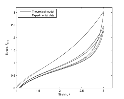
Figure 3: Comparison of our theoretical model with experimental data of Dorfmann & Ogden (2004), transversely isotropic model, particle-reinforced specimen with 20 phr of carbon black.

Figure 4 has been obtained by applying the following constants and functions,

$$N=5.5,\quad\mu=1.41,\quad r_{1}=r_{2}=1.14,\quad\alpha^{2}=0.8,\quad a_{1}=0.4,$$

$${A}_{0}=-0.01,\quad{A_{1,2}}(t)=-0.067\log(t),\quad{A_{4,5}}(t)=0,\quad a(t)=H(t-t_{1})t,$$

$$\zeta_{0}^{\phantom{*}}(\lambda)=1-0.840\left[\mathrm{\tanh\,}(3-\lambda)\right]^{3.2},$$

$$d_{\omega}=\left\{\begin{array}[]{clrr}0.020\\ 0.012\\ \end{array}\right.\mu b_{\omega}=\left\{\begin{array}[]{clrr}1.14\\ 2.48\\ \end{array}\right.\vartheta_{\omega}=\left\{\begin{array}[]{clrr}0.70\\ 1.00\\ \end{array}\right.s_{1}=\left\{\begin{array}[]{clrr}2.60\\ 2.60\\ \end{array}\right.s_{2}=\left\{\begin{array}[]{clrr}-0.2&\textrm{unloading},\\ -0.2&\textrm{loading}.\\ \end{array}\right.$$

Figure 4 shows that the transversely isotropic model provides a good fit with experimental data and is a significant improvement on the isotropic model of (Rickaby & Scott, 2013, Figure 16). The better fit here is partly due to the modelling of stress-softening on the primary loading path.

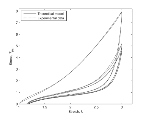
Figure 4: Comparison of our theoretical model with experimental data of Dorfmann & Ogden (2004), transversely isotropic model, particle-reinforced specimen with 60 phr of carbon black.

9 Conclusions

This model appears to be the first appearance in the literature of a transversely isotropic stress-softening and residual strain model which has been combined with a transversely isotropic version of the Arruda-Boyce eight-chain constitutive model of elasticity in order to develop a model that is capable of accurately representing the Mullins effect in uniaxial tension when compared with experimental data.

The model has been developed is such a way that any of the salient inelastic features could be excluded and the integrity of the model would still be maintained. The proposed model should prove extremely effective in the modelling of many practical applications.

Figures 3 and 4 provide a comparison between experimental the data of Dorfmann & Ogden (2004) and the transversely isotropic model presented here. By comparing Figures 3 and (Rickaby & Scott, 2013, Figure 15) it can be seen that the present transversely isotropic model provides a much better fit to the data than does the original isotropic model of Rickaby & Scott (2013). Similarly, for the higher concentration of carbon black of Figures 4 comparing with (Rickaby & Scott, 2013, Figure 16) shows that the transversely isotropic model provides an equally better fit. This is partly due to the new feature of the modelling of stress-softening on the primary loading path.

After an applied uniaxial deformation, the induced transverse isotropy means that the directions perpendicular and parallel to the deformation have sustained different degrees of damage which is borne out by the experimental data of (Diani et al., 2006, Figure 3). Thus, whilst some of the material parameters of our model remain the same along the direction of uniaxial tension and perpendicular to it, the anisotropic terms, in particular the stress-relaxation terms, may not necessarily be equal for two perpendicular directions.

Our present model can be modified to cope with multiple stress/strain cycles, with increasing values of maximum stretch, and we hope to present a comparison between theory and experiment at a later date.

The version of the model developed here is for uniaxial tension. We expect that the results presented here could be extended to include equibiaxial tension, pure or simple shear, and a general three-dimensional model. These ideas will be developed in later papers.

A further application of the model could be to the mechanics of soft biological tissue. The comparison between the stress-softening associated with soft biological tissue, in particular muscle, and filled vulcanizated rubber has been discussed in detail by (Dorfmann et al., 2007, Section 2). For cyclic stress softening both materials exhibit stress relaxation, hysteresis, creep and creep of residual strain. Similar observations have been made for arterial material, see for example Holzapfel et al. (2000). After preliminary investigations it is apparent that the model presented here could be extended to include biological soft tissue, though the inherent anisotropy of biological tissue would need to be taken into consideration.

References

• Arruda & Boyce (1993) Arruda, E. M. & Boyce, M. C. (1993). A three-dimensional constitutive model for the large stretch behavior of rubber elastic materials. J. Mech. Phys. Solids, 41, 389–412.
• Bergström & Boyce (1998) Bergström, J. S. & Boyce, M. C. (1998). Constitutive modelling of the large strain time-dependent behavior of elastomers. J. Mech. Phys. Solids, 46, 931–954.
• Bernstein et al. (1963) Bernstein, B., Kearsley, E. A., & Zapas, L. J. (1963). A Study of Stress Relaxation with Finite Strain. Trans. Soc. Rheology VII, 71, 391–410.
• Cohen (1991) Cohen, A. (1991). A Padé approximation to the inverse Langevin function. Rheol. Acta, 30, 270–273.
• Diani et al. (2006) Diani, J., Brieu, M., & Gilormini, P. (2006). Observation and modeling of the anisotropic visco-hyperelastic behavior of a rubberlike material. Int. J. Solids Structures, 43, 3044–3056.
• Diani et al. (2009) Diani, J., Fayolle, B., & Gilormini, P. (2009). A review on the Mullins effect. Eur. Polym. J., 45, 601–612.
• Dorfmann & Ogden (2003) Dorfmann, A. & Ogden, R. W. (2003). A pseudo-elastic model for loading, partial unloading and reloading of particle-reinforced rubber. Int. J. Solids Structures, 40, 2699–2714.
• Dorfmann & Ogden (2004) Dorfmann, A. & Ogden, R. W. (2004). A constitutive model for the Mullins effect with permanent set in particle-reinforced rubber. Int. J. Solids Structures, 41, 1855–1878.
• Dorfmann & Pancheri (2012) Dorfmann, A. & Pancheri, F. Q. (2012). A constitutive model for the Mullins effect with changes in material symmetry. Int. J. Non-Linear Mech., 47, 874–887.
• Dorfmann et al. (2007) Dorfmann, A., Trimmer, B. A., & Woods, W. A. (2007). A constitutive model for muscle properties in a soft-bodied arthropod. J. R. Soc. Interface, 4, 257–269.
• Gent (1996) Gent, A. N. (1996). A new constitutive relation for rubber. Rubber Chem. Technol., 69, 59–61.
• Holzapfel et al. (2000) Holzapfel, G. A., Gasser, T. C., & Ogden, R. W. (2000). A New Constitutive Framework for Arterial Wall Mechanics and a Comparative Study of Material Models. J. Elasticity, 61, 1–48.
• Horgan & Saccomandi (2002) Horgan, C. O. & Saccomandi, G. (2002). A Molecular-Statistical Basis for the Gent Constitutive Model of Rubber Elasticity. J. Elasticity, 68, 167–176.
• Horgan et al. (2004) Horgan, C. O., Ogden, R. W., & Saccomandi, G. (2004). A theory of stress softening of elastomers based on finite chain extensibility. Proc. R. Soc. Lond. A, 460, 1737–1754.
• Kuhl et al. (2005) Kuhl, E., Garikipati, K., Arruda, E. M., & Grosh, K. (2005). Remodeling of biological tissue: Mechanically induced reorientation of a transversely isotropic chain network. J. Mech. Phys. Solids, 53, 1552–1573.
• Lockett (1972) Lockett, F. J. (1972). Nonlinear Viscoelastic Solids. Academic Press, London.
• Merodio & Ogden (2005) Merodio, J. & Ogden, R. W. (2005). Mechanical response of fiber-reinforced incompressible non-linear elastic solids. Int. J. Non-Linear Mech., 40, 213–227.
• Mullins (1947) Mullins, L. (1947). Effect of stretching on the properties of rubber. J. Rubber Research, 16(12), 275–289.
• Mullins (1969) Mullins, L. (1969). Softening of rubber by deformation. Rubber Chem. Technol., 42(1), 339–362.
• Ogden & Roxburgh (1999) Ogden, R. W. & Roxburgh, D. G. (1999). A pseudo-elastic model for the Mullins effect in filled rubber. Proc. R. Soc. Lond. A, 455, 2861–2877.
• Park & Hamed (2000) Park, B. & Hamed, G. R. (2000). Anisotropy in Gum and Black Filled SBR and NR Vulcanizates Due to Large Deformations. Korea Polym. J., 8, 268–275.
• Rickaby & Scott (2011) Rickaby, S. R. & Scott, N. H. (2011). The Mullins effect. Constitutive Models for Rubber VII, Taylor $\&$ Francis Group, London, pages 273–276.
• Rickaby & Scott (2013) Rickaby, S. R. & Scott, N. H. (2013). A cyclic stress softening model for the Mullins effect. Int. J. Solids Structures., 50, 111–120.
• Spencer (1984) Spencer, A. J. M. (1984). Constitutive theory for strongly anisotropic solids. In A. J. M. Spencer, editor. Continuum Theory of the Mechanics of Fibre-Reinforced Composites, pages 1–32. CISM Courses and Lectures No. 282.
• Tanner (1988) Tanner, R. I. (1988). From A to (BK)Z in constitutive relations. J. Rheol., 32, 673–702.
• Tommasi et al. (2006) Tommasi, D. D., Puglisi, G., & Saccomandi, G. (2006). A micromechanics-based model for the Mullins effect. J. Rheol., 50(4), 495–512.
• Wineman (2009) Wineman, A. (2009). Nonlinear Viscoelastic Solids — A Review. Math. Mech. Solids, 14, 300–366.