Non-Markovian Sensing of a Quantum Reservoir

Abstract

Quantum sensing explores protocols using the quantum resource of sensors to achieve highly sensitive measurement of physical quantities. The conventional schemes generally use unitary dynamics to encode quantities into sensor states. In order to measure the spectral density of a quantum reservoir, which plays a vital role in controlling the reservoir-caused decoherence to microscopic systems, we propose a nonunitary-encoding optical sensing scheme. Although the nonunitary dynamics for encoding in turn degrades the quantum resource, we surprisingly find a mechanism to make the encoding time a resource to improve the precision and to make the squeezing of the sensor a resource to surpass the shot-noise limit. Our result shows that it is due to the formation of a sensor-reservoir bound state. Enriching the family of quantum sensing, our scheme gives an efficient way to measure the quantum reservoir and might supply an insightful support to decoherence control.

I Introduction

Quantum sensing pursues highly precise measuring of physical quantities by using quantum effects of sensors in specific encoding and measurement protocols Degen et al. (2017); Pezzè et al. (2018); Sidhu and Kok (2020); Lachance-Quirion et al. (2020). The precision of any measurement obeying classical physics is bounded by the shot-noise limit (SNL). Quantum sensing allows us to attain a precision that surpasses the SNL by using quantum resources, such as entanglement Megidish et al. (2019); Zhang et al. (2018); Unternährer et al. (2018); Zou et al. (2018); Nagata et al. (2007); Daryanoosh et al. (2018) and squeezing Caves (1981); Engelsen et al. (2017); Nolan et al. (2017). It has inspired many fascinating applications in gravitational wave detection Tse et al. (2019); Acernese et al. (2019), quantum radar Cohen et al. (2019); Gregory et al. (2020), ultimate clocks Kómár et al. (2014); Kruse et al. (2016); Hosten et al. (2016), quantum magnetometry Muessel et al. (2014); Bonato et al. (2016) and optical lithography Pavel et al. (2013). These sensing schemes commonly resort the unitary dynamics of the sensors to encode the quantities into the sensor states. It is applicable only to measure classical systems Zhuang and Zhang (2019); Gessner et al. (2019); Chu et al. (2020); Lupo et al. (2020); Wang et al. (2019); Gatto et al. (2019); McCormick et al. (2019); Chabuda et al. (2020); Yu et al. (2020); Haase et al. (2018); Bai et al. (2019); Górecki et al. (2020); Kura and Ueda (2020); Che et al. (2019); Tatsuta et al. (2019). To sense a quantum system, the quantized sensor-system coupling for encoding the quantities definitely makes the dynamics of the sensor nonunitary. A natural question is: how can one generalize the well-developed unitary-encoding quantum sensing schemes to the nonunitary case?

Recently, there is an increasing motivation to develop the nonunitary quantum sensing scheme, especially in the setting of measuring a quantum reservoir. The inevitable interactions with the reservoir would cause any microscopic system to lose its quantum coherence, which is called decoherence and is a main bottleneck to realize quantum computers and other quantum tasks Rivas et al. (2014); Breuer et al. (2016); de Vega and Alonso (2017); Li et al. (2018). Characterizing the system-reservoir coupling strength in different reservoir frequencies, the spectral density completely determines the decoherence. The full grasping to the features of the spectral density is a prerequisite for understanding Mascherpa et al. (2017) and controlling Kofman and Kurizki (2001) the decoherence. However, in many situations, the spectral density cannot be microscopically derived from first principles Leggett et al. (1987); Yang et al. (2016). Thus, a measuring of the spectral density is strongly necessary. Inspired by the high-precision nature of quantum sensing, several schemes have been proposed to measure the spectral density Mascherpa et al. (2017); Goldwater et al. (2019); Farfurnik and Bar-Gill (2020); Benedetti et al. (2018); Bina et al. (2018); Tamascelli et al. (2020); Sehdaran et al. (2019); Gebbia et al. (2020). A substantial difference of these schemes from the previous ones Zhuang and Zhang (2019); Gessner et al. (2019); Chu et al. (2020); Lupo et al. (2020); Wang et al. (2019); Gatto et al. (2019); McCormick et al. (2019); Chabuda et al. (2020); Yu et al. (2020); Haase et al. (2018); Bai et al. (2019); Górecki et al. (2020); Kura and Ueda (2020); Che et al. (2019); Tatsuta et al. (2019) resides in that the quantities are encoded into the sensor state via nonunitary dynamics, which in turn degrades the quantum resources of the sensors. This is expected to deteriorate the performance of the sensing schemes with increasing the encoding time. We see in Ref. Benedetti et al. (2018); Bina et al. (2018); Tamascelli et al. (2020); Sehdaran et al. (2019); Gebbia et al. (2020) that the sensing precision to the spectral density not only does not surpass the SNL, but also gets worse and worse with increasing the encoding time. Thus, how to surpass the SNL in the long encoding time condition is still an open question in sensing a quantum reservoir.

We here propose a nonunitary sensing scheme using a quantized single-mode optical field as a sensor to estimate the spectral density of a quantum reservoir. A mechanism to make the encoding time and the optical squeezing resources to surpass the SNL at any long encoding time is present based on the non-Markovian description of the nonunitary encoding dynamics. Our analysis reveals that the proposed mechanism works efficiently due to the formation of a bound state in the energy spectrum of the composite system consisting of the optical sensor and the reservoir. With this mechanism, our scheme eliminates the outstanding error-divergence problem of sensing the quantum reservoir in the long encoding time regime.

II Quantum parameter estimation

To estimate the quantity $\theta$ of a system, we first prepare a quantum sensor in the state $\varrho_{\text{in}}$ and couple it to the system to encode $\theta$ into the sensor state $\varrho_{\theta}$. Then we measure certain sensor observables and infer the value of $\theta$ from the result. The inevitable errors make us unable to estimate $\theta$ precisely. According to quantum parameter estimation theory Liu et al. (2019); Braunstein and Caves (1994), the ultimate precision of $\theta$ is constrained by the quantum Cramér-Rao bound $\delta\theta\geq 1/\sqrt{\upsilon\mathcal{F}_{\theta}}$, where $\delta\theta$ is the standard error of the estimate, $\upsilon$ is the number of repeated measurements, and $\mathcal{F}_{\theta}=\text{Tr}(\hat{L}_{\theta}^{2}\varrho_{\theta})$ with $\hat{L}_{\theta}$ defined by $\partial_{\theta}\varrho(\theta)=(\hat{L}_{\theta}\varrho_{\theta}+\varrho_{\theta}\hat{L}_{\theta})/2$ is the quantum Fisher information (QFI) characterizing the most information of $\theta$ extractable from $\varrho_{\theta}$. We set $\upsilon=1$ due to the independence of $\mathcal{F}_{\theta}$ on $\upsilon$. How to maximize the QFI by resorting to the proper initial state $\varrho_{\text{in}}$ and sensor-system interaction is of importance in quantum sensing. If $\delta\theta$ is proportional to $\bar{n}^{-1/2}$ or $\mathcal{F}_{\theta}\propto\bar{n}$, with $\bar{n}$ being the number of the used resource, then the precision is called the SNL. The SNL can be beaten by using quantum protocols Zhuang and Zhang (2019); Gessner et al. (2019); Chu et al. (2020); Lupo et al. (2020); Wang et al. (2019); Gatto et al. (2019); McCormick et al. (2019); Chabuda et al. (2020); Yu et al. (2020); Haase et al. (2018); Bai et al. (2019); Górecki et al. (2020); Kura and Ueda (2020); Che et al. (2019); Tatsuta et al. (2019).

III Quantum sensing to a dissipative reservoir

We are interested in uncovering the quantum superiority in sensing a quantum reservoir with infinite degrees of freedom. We choose a single-mode optical field as the quantum sensor and utilize the following sensor-reservoir coupling to encode the reservoir quantities into the sensor ($\hbar=1$):

$$\hat{H}=\omega_{0}\hat{a}^{\dagger}\hat{a}+\sum_{k}\omega_{k}\hat{b}_{k}^{\dagger}\hat{b}_{k}+\sum_{k}g_{k}\big{(}\hat{a}\hat{b}_{k}^{\dagger}+\hat{a}^{\dagger}\hat{b}_{k}\big{)},$$ (1)

where $\hat{a}$ and $\hat{b}_{k}$ are the annihilation operators of the sensor with frequency $\omega_{0}$ and the $k$th reservoir mode with frequency $\omega_{k}$, respectively, and $g_{k}$ is the sensor-reservoir coupling strength. Depending on the properties of the reservoir, the coupling is characterized by the spectral density in the continuum limit of the frequency $J(\omega)\equiv\sum_{k}g_{k}^{2}\delta(\omega-\omega_{k})=g(\omega)^{2}D(\omega)$, where $D(\omega)=\int dk/d\omega_{k}\delta(\omega-\omega_{k})d\omega$, called the density of state, depends on the dispersion relation of the reservoir.

Using the Feynman-Vernon’s influence functional method to trace over the state of the reservoir An and Zhang (2007); Zhang et al. (2012); Yang et al. (2014), we derive the non-Markovian master equation of the sensor:

$$\dot{\varrho}(t)=-i\Omega(t)\big{[}\hat{a}^{\dagger}\hat{a},\varrho(t)\big{]}+\Gamma(t)\check{\mathcal{L}}[\varrho(t)],$$ (2)

where $\check{\mathcal{L}}[\cdot]=2\hat{a}\cdot\hat{a}^{\dagger}-\{\hat{a}^{\dagger}\hat{a},\cdot\}$, $\Omega(t)\equiv-\mathrm{Im}[{\dot{u}}(t)/u(t)]$ is the renormalized frequency, and $\Gamma(t)\equiv-\mathrm{Re}[\dot{u}(t)/u(t)]$ is a time-dependent dissipation coefficient. The reservoir is assumed in vacuum initially and $u(t)$ is determined by

$$\dot{u}(t)+i\omega_{0}u(t)+\int_{0}^{t}\nu(t-\tau)u(\tau)d\tau=0,$$ (3)

with $u(0)=1$ and $\nu(x)=\int_{0}^{\infty}J(\omega)e^{-i\omega x}d\omega$. Keeping the same Lindblad form as the Markovian master equation, Eq. (2) collects the non-Markovian effect in the time-dependent coefficients. We see from Eq. (3) that $J(\omega)$ has been successfully encoded into $\varrho(t)$ by Eq. (2).

Different from the widely used unitary evolution Zhuang and Zhang (2019); Gessner et al. (2019); Chu et al. (2020); Lupo et al. (2020); Wang et al. (2019); Gatto et al. (2019); McCormick et al. (2019); Chabuda et al. (2020); Yu et al. (2020); Haase et al. (2018); Bai et al. (2019); Górecki et al. (2020); Kura and Ueda (2020); Che et al. (2019); Tatsuta et al. (2019), the quantity encoding governed by Eq. (2) is a nonunitary dynamics of the sensor. Although it would cause decoherence to the sensor, we still can estimate the quantities in $J(\omega)$ in higher precision than the classical SNL via properly utilizing the quantum characters of the sensor. We consider the initial state of the sensor as the squeezed state $\varrho(0)=\hat{\mathcal{D}}(\alpha)\hat{\mathcal{S}}(r)|0\rangle\langle 0|\hat{\mathcal{S}}^{\dagger}(r)\hat{\mathcal{D}}^{\dagger}(\alpha)$, where $\hat{\mathcal{D}}(\alpha)=\exp(\alpha\hat{a}^{\dagger}-\alpha^{*}\hat{a})$ and $\hat{\mathcal{S}}(r)=\exp[r(\hat{a}^{2}-\hat{a}^{{\dagger}2})/2]$, with $|0\rangle$ being the vacuum state. The total photon number $\bar{n}=|\alpha|^{2}+\sinh^{2}r$, which contains the ratio $\beta\equiv\sinh^{2}r/\bar{n}$ from the squeezing of the optical sensor and is regarded as the quantum resource of the scheme. The ratio $\beta$ varies from $0$ for a coherent state to $1$ for a squeezed vacuum state. The Gaussianity of the initial state is preserved during the evolution governed by Eq. (2). The Gaussian states are those whose characteristic function is of Gaussian form Braunstein and van Loock (2005); Šafránek et al. (2015) $\chi({\boldsymbol{\gamma}})\equiv\text{Tr}[\varrho\hat{\mathcal{D}}({\gamma})]=\exp[-{\frac{1}{4}}{\boldsymbol{\gamma}}^{{\dagger}}{\boldsymbol{\sigma}}{\boldsymbol{\gamma}}-i{\mathbf{d}}^{{\dagger}}K{\boldsymbol{\gamma}}]$, where ${\boldsymbol{\gamma}}=(\gamma,\gamma^{*})^{T}$, $K=\text{diag}(1,-1)$, and the elements of the displacement vector ${\mathbf{d}}$ and the covariant matrix ${\boldsymbol{\sigma}}$ are $d_{i}=\text{Tr}[\varrho\hat{A}_{i}]$ and $\sigma_{ij}=\text{Tr}[\varrho\{\Delta\hat{A}_{i},\Delta\hat{A}_{j}^{{\dagger}}\}]$ with $\hat{\mathbf{A}}=(\hat{a},\hat{a}^{\dagger})^{T}$ and $\Delta\hat{A}_{i}=\hat{A}_{i}-d_{i}$. The QFI for $\theta$ in $\varrho$ reads Šafránek (2019); Šafránek et al. (2015); Gao and Lee (2014)

$$\mathcal{F}_{\theta}=\frac{1}{2}[\text{vec}(\partial_{\theta}{\boldsymbol{\sigma}})]^{\dagger}\mathcal{M}^{-1}\text{vec}(\partial_{\theta}{\boldsymbol{\sigma}})+2(\partial_{\theta}\mathbf{d})^{\dagger}\boldsymbol{\sigma}^{-1}\partial_{\theta}\mathbf{d},$$ (4)

where $\mathcal{M}={\boldsymbol{\sigma}}^{*}\otimes{\boldsymbol{\sigma}}-K\otimes K$, with $\boldsymbol{\sigma}^{*}$ being the complex conjugate of $\boldsymbol{\sigma}$.

Taking the Ohmic-family spectral density $J(\omega)=\eta\omega(\omega/\omega_{c})^{s-1}e^{-\omega/\omega_{c}}$ as an example, we reveal the performance of our non-Markovian sensing scheme. The dimensionless constant $\eta$ characterizes the sensor-reservoir coupling strength, the cutoff frequency $\omega_{c}$ characterizes the correlation time scale of the reservoir, and the exponent $s$ relating to the spatial dimension classifies the reservoir into sub-Ohmic when $0<s<1$, Ohmic when $s=1$, and super-Ohmic when $s>1$ Leggett et al. (1987). They are the parameters we estimate from $\varrho(t)$. Solving Eq. (2), we obtain Sup

$$\mathbf{d}(t) = [\alpha u(t),\alpha^{*}u^{*}(t)]^{T},$$ (5)

$$\boldsymbol{\sigma}(t) = \left[\begin{array}[]{cc}1+2|u(t)|^{2}\sinh^{2}r&-u(t)^{2}\sinh(2r)\\ -u^{*}(t)^{2}\sinh(2r)&1+2|u(t)|^{2}\sinh^{2}r\\ \end{array}\right].$$ (8)

Then the QFI of the parameters in $J(\omega)$ can be calculated.

When the sensor-reservoir coupling is weak and the correlation time scale of the reservoir is smaller than that of the sensor, we apply the Markovian approximation to Eq. (3) and obtain $u_{\text{MA}}(t)=e^{-[\kappa+i(\omega_{0}+\Delta(\omega_{0}))]t}$, with $\kappa=\pi J(\omega_{0})$ and $\Delta(\omega_{0})=\mathcal{P}\int_{0}^{\infty}{J(\omega)\over\omega_{0}-\omega}d\omega$. It causes $\Gamma_{\text{MA}}(t)=\kappa$ and $\Omega_{\text{MA}}(t)=\omega_{0}+\Delta(\omega_{0})$ Yang et al. (2014), which are equal to the ones in the Markovian master equation. The Markovian approximate QFI in the large-$\bar{n}$ limit reads

$$\mathcal{F}^{\text{MA}}_{\theta}(t)=2(1-\beta)(\partial_{\theta}\kappa)^{2}[\coth(\kappa t)-1]\bar{n}t^{2},$$ (9)

where $\theta=\eta$, $\omega_{c}$, or $s$. We have neglected the constant $\Delta(\omega_{0})$, which is generally renormalized into $\omega_{0}$ Leggett et al. (1987). One can see from Eq. (9) that $\lim_{t\rightarrow\infty}\mathcal{F}^{\text{MA}}_{\theta}(t)=0$, which indicates that no information on $\theta$ is extractable from $\varrho(\infty)$, and thus the scheme breaks down in the long-encoding time condition. This is physically understandable because the steady state of Eq. (2) under the Markovian approximation uniquely being the vacuum state $\varrho(\infty)=|0\rangle\langle 0|$ does not carry any message on $J(\omega)$. However, after optimizing $\mathcal{F}^{\text{MA}}_{\theta}(t)$ to time, we have

$$\max\mathcal{F}^{\text{MA}}_{\theta}\simeq 0.65(\partial_{\theta}\ln\kappa)^{2}\bar{n}$$ (10)

when $t\simeq 0.80\kappa^{-1}$. The maximum (10) is achieved when $\beta=0$ for the input state is the coherent state. This implies that no quantum superiority is delivered by the squeezing. The scaling relation of $\max\mathcal{F}^{\text{MA}}_{\theta}$ to $\bar{n}$ equals exactly to the classical SNL.

In the non-Markovian dynamics, the analytical QFI is complicated. We leave it to the numerical calculation. However, via analyzing the long-time behavior of $u(t)$, we may obtain an asymptotic form of QFI. A Laplace transform can convert Eq. (3) into $\tilde{u}(z)=[z+i\omega_{0}+\int_{0}^{\infty}{J(\omega)\over z+i\omega}d\omega]^{-1}$. The solution of $u(t)$ is obtained by the inverse Laplace transform of $\tilde{u}(z)$, which can be done by finding its pole from

$$y(E)\equiv\omega_{0}-\int_{0}^{\infty}{J(\omega)\over\omega-E}d\omega=E,~{}(E=iz).$$ (11)

Note that the roots $E$ of Eq. (11) are just the eigenenergies of Eq. (1) in the single-excitation space. Specifically, expanding the eigenstate as $|\Psi\rangle=(x\hat{a}^{\dagger}+\sum_{k}y_{k}\hat{b}_{k}^{\dagger})|0,\{0_{k}\}\rangle$ and substituting it into $\hat{H}|\Psi\rangle=E|\Psi\rangle$, with $E$ being the eigenenergy, we have $(E-\omega_{0})x=\sum_{k}g_{k}y_{k}$ and $y_{k}=g_{k}x/(E-\omega_{k})$. They readily lead to Eq. (11). It reveals that, although the spaces with any excitation numbers are involved, the dynamics is uniquely determined by the energy spectrum in the single-excitation space. Since $y(E)$ is a decreasing function in the regime $E<0$, Eq. (11) has one isolated root $E_{b}$ in this regime provided $y(0)<0$. While $y(E)$ is ill defined when $E>0$, Eq. (11) has infinite roots in this regime forming a continuous energy band. We call the eigenstate of the isolated eigenenergy $E_{b}$ the bound state Bai et al. (2019). After the inverse Laplace transform, we obtain Sup

$$u(t)=Ze^{-iE_{b}t}+\int_{0}^{\infty}\frac{J(E)e^{-iEt}dE}{[E-\omega_{0}-\Delta(E)]^{2}+[\pi J(E)]^{2}},$$ (12)

where the first term with $Z=[1+\int_{0}^{\infty}{J(\omega)d\omega\over(E_{b}-\omega)^{2}}]^{-1}$ is from the bound state, and the second one is from the band energies. Oscillating with time in continuously changing frequencies, the integral tends to zero in the long-time condition due to out-of-phase interference. Thus, if the bound state is absent, then $\lim_{t\rightarrow\infty}u(t)=0$ characterizes a complete decoherence, while if the bound state is formed, then $\lim_{t\rightarrow\infty}u(t)=Ze^{-iE_{b}t}$ implies a decoherence suppression. We can evaluate that the bound state for the Ohmic-family spectral density is formed if $\omega_{0}\leq\eta\omega_{c}\underline{\Gamma}(s)$, where $\underline{\Gamma}(s)$ is the Euler’s gamma function.

In the absence of the bound state, it is natural to expect that $\mathcal{F}_{\theta}(t)$ tends to zero because $u(t)$ approaches zero. Consistent with the Markovian result, the sensing scheme in this case also breaks down. In the presence of the bound state, we substitute the long-time $u(t)$ into Eq. (4) and obtain Sup

$$\mathcal{F}_{\theta}(t)\simeq 4Z^{2}\Theta(\beta,\bar{n})(\partial_{\theta}E_{b})^{2}t^{2}$$ (13)

with $\Theta(\beta,\bar{n})=\frac{\bar{n}(1-\beta)[1-2Z^{2}(\sqrt{\bar{n}\beta(1+\bar{n}\beta)}-\bar{n}\beta)]}{1+4\bar{n}\beta Z^{2}(1-Z^{2})}+\frac{2Z^{2}\bar{n}\beta(1+\bar{n}\beta)}{1+2\bar{n}\beta Z^{2}(1-Z^{2})}$. In the case of $\beta=0$, we have $\Theta(0,\bar{n})=\bar{n}$. In the general case, $\Theta(\beta,\bar{n})\simeq{\bar{n}\beta\over 1-Z^{2}}$ can be derived in the large-$\beta\bar{n}$ limit. It is remarkable to find that, in contrast to the cases of Markovian approximation and without the bound state, $\mathcal{F}_{\theta}(t)$ in the non-Markovian dynamics increases with time in power law when the bound state is formed. The scaling of $\mathcal{F}_{\theta}(t)$ to time is the same as the ideal Ramsey-spectroscopy based quantum metrology, where the parameter encoding is via unitary dynamics Huelga et al. (1997); Gefen et al. (2019). The result reveals that, thanks to the bound state, even the parameters are encoded via nonunitary dynamics with the decoherence presented, the sensing to the reservoir still performs as ideal as the unitary-encoding scheme. Furthermore, although scaling with $\bar{n}$ in a manner similar to that of the SNL achieved by the coherent state $\beta=0$, QFI still has a dramatic prefactor improvement by the optimal squeezing $\beta=1$. Therefore, the bound state has made both the encoding time and the squeezing act as resources in our sensing scheme.

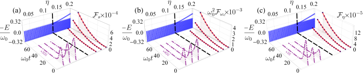
Figure 1: Evolution of $\mathcal{F}_{\theta}(t)$ in different $\eta$ obtained by numerically solving Eq. (3). The purple dot-dashed lines are magnified by the times marked in the plots. The blue dots are the energy spectrum of the total system consisting of the sensor and the reservoir. The darker-blue dots represent the analytical results from Eq. (13), which are in good agreement with the numerical results. The parameters $\omega_{c}=4.5\omega_{0}$, $s=0.5$, $\bar{n}=100$, and $\beta=0.5$ are used.

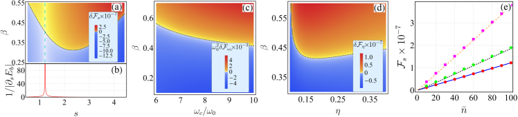
Figure 2: (a,c,d) $\delta\mathcal{F}_{\theta}(40\omega_{0}^{-1})$ as a function of $\beta$ and $\theta=s$, $\omega_{c}$ and $\eta$. The dotted lines are analytically evaluated from $\Theta(\beta,\bar{n})=\bar{n}$. (b) A singular point of the $\mathcal{F}_{s}$ is present at $s\simeq 1.2$. (e) $\mathcal{F}_{s}(40\omega_{0}^{-1})$ as the change of $n$ when $\beta=0$ (solid line), $0.5$ (dotted line), and $1$ (dot-dashed line). The circles, diamonds, and squares are analytically obtained from Eq. (13). The parameters $(\eta,\omega_{c})=(0.4,10\omega_{0})$ in panels (a) and (b), $(\eta,s)=(0.2,1)$ in panel (c), $(s,\omega_{c})=(1,10\omega_{0})$ in panel (d), and $(\eta,s,\omega_{c})=(0.4,3,10\omega_{0})$ in panel (e) are used.

IV Numerical results

To verify our non-Markovian sensing scheme, we present numerical simulations of the dynamics of QFI. In Fig. 1, we plot the evolution of the QFI for $\theta=s$, $\omega_{c}$, and $\eta$ in different $\eta$. We see that, in the regime $\eta\lesssim 0.13$ where the bound state is absent, $\mathcal{F}_{\theta}(t)$ quickly increase to their maxima, and then decrease to zero as time increases. Here the reservoir causes the sensor to undergo a complete decoherence such that its quantum characters are fulled destroyed. This is qualitatively consistent with the Markovian approximate result in Eq. (9) and the previous works Benedetti et al. (2018); Bina et al. (2018); Tamascelli et al. (2020); Sehdaran et al. (2019); Gebbia et al. (2020). On the contrary, $\mathcal{F}_{\theta}(t)$ monotonically increase with time when $\eta\gtrsim 0.13$ where the bound state is formed. Well matching the analytical result in Eq. (13) (see the darker-blue dots), $\mathcal{F}_{\theta}(t)$ in this regime exhibit a square power law with the encoding time. Such law is achievable only in the unitary-encoding quantum metrology in the ideal case Huelga et al. (1997); Gefen et al. (2019). It indicates that although the nonunitary encoding can cause decoherence to the sensor, we still have the chance to obtain a precision scaling with time as ideal as the unitary encoding scheme. Different from many previous studies on sensing a reservoir Benedetti et al. (2018); Bina et al. (2018); Tamascelli et al. (2020); Sehdaran et al. (2019); Gebbia et al. (2020) in which the precision becomes worse as time increases, our result reveals a mechanism to make the encoding time as a resource in improving the precision. It demonstrates the distinguished role played by the bound state in boosting the QFI of our non-Markovian quantum sensing scheme.

Another role of the bound state is that it permits us to obtain a higher precision than the SNL via optimizing the quantum resource. We define $\delta\mathcal{F}_{\theta}(t)\equiv\mathcal{F}_{\theta}(t)-\mathcal{F}_{\theta}(t)|_{\beta=0}$ as a witness to quantify the effect of squeezing. Focusing on the regime in the presence of the bound state, we obtain $\delta\mathcal{F}_{\theta}(t)=4Z^{2}t^{2}(\partial_{\theta}E_{b})^{2}[\Theta(\bar{n},\beta)-\bar{n}]$ from Eq. (13). It can be seen that the precision goes beyond the benchmarked SNL achieved by the coherent state as long as $\Theta(\bar{n},\beta)>\bar{n}$. Figure 2(a) shows the exact long-time $\delta\mathcal{F}_{s}(t)$ in different $\beta$ and $s$. We really observe a clear threshold perfectly matching the analytical criterion $\Theta(\beta,\bar{n})=\bar{n}$, above which the SNL is surpassed. An exception occurs at $s\simeq 1.2$, where $\partial_{\theta}E_{b}=0$ [see Fig. 2(b)]. Such singular point is called Rayleigh’s curse Gefen et al. (2019); Tsang et al. (2016); Zhou and Jiang (2019), which sets a limit on the optical-imaging resolution. The same result of squeezing-enhanced precision is confirmed by $\delta\mathcal{F}_{\omega_{c}}$ in Fig. 2(c) and $\delta\mathcal{F}_{\eta}$ in Fig. 2(d). The behavior of $\mathcal{F}_{s}$ as the change of $\bar{n}$ in Fig. 2(e) verifies that, although the long-time QFI has the same scaling relation to $\bar{n}$ with the SNL, a sufficient room to boost the QFI by the prefactor still exists. All these numerical results verify our conclusion that the squeezing can enhance the precision to sense the reservoir.

V Discussion and conclusions

Our conclusion in Eq. (13) is independent of the form of spectral density. Although only the Ohmic-family form is considered, our result is generalizable to other cases, where the specific condition of forming a bound state might be different, but the conclusion remains unchanged. The non-Markovian effect has been observed in optical and optomechanical systems Liu et al. (2011); Bernardes et al. (2015); Gröblacher et al. (2015). The bound state and its effect on the open-system dynamics have been observed in circuit QED Liu and Houck (2017) and ultracold atom Krinner et al. (2018) systems. These progresses provide a strong support to our scheme. We can verify our conclusion by using the experimental parameters in Ref. Liu and Houck (2017), as shown in the Supplemental Material Sup . It indicates that our finding is realizable in the state-of-the-art technique of quantum optics experiments. Our result could be generalized to the finite-temperature reservoir case, where the impact of the bound state on the equilibration dynamics has been found Yang et al. (2014). Although our result cannot give the optimal measurement observable, the superiority of our bound-state-favored sensing scheme can be demonstrated via a measurement protocol Sup . Note that our work has substantial differences from Ref. Bai et al. (2019). First, the reservoir here is the target to which we intend to actively measure, while the one in Ref. Bai et al. (2019) is the source that passively causes unwanted detrimental influence on the ideal unitary-encoding metrology scheme. Second, our goal here is to achieve a high-precision sensing of a reservoir and eliminate the outstanding error-divergence problem, while Ref. Bai et al. (2019) concentrates on how to retrieve the ideal performance of a quantum metrology scheme from the influence of decoherence.

In summary, we have proposed an optical sensing scheme to estimate the spectral density of a quantum reservoir. A threshold, above which the QFI scales with the encoding time in the same square power law as the noiseless Ramsey-spectroscopy metrology scheme, is found. This is in contrast to the result in the Markovian approximation and the previous works  Benedetti et al. (2018); Bina et al. (2018); Tamascelli et al. (2020); Sehdaran et al. (2019); Gebbia et al. (2020) that the precision gets deteriorated with time. It is due to constructive interplay between the non-Markovian effect and the sensor-reservoir bound state: The bound state supplies the intrinsic ability and the non-Markovian effect supplies the dynamical way to achieve the good performance of our nonunitary-encoding sensing scheme. We further find that such interplay can also permit us to achieve a prefactor surpassing the SNL by the squeezing of the sensor. Paving a way to realize a high-precision sensing to the quantum reservoir by the nonunitary-dynamics encoding, our result is helpful in understanding and controlling decoherence caused by the reservoir.

VI Acknowledgments

The work is supported by the National Natural Science Foundation (Grants No. 11704025, No. 11875150, and No. 11834005).

References

- Degen et al. (2017) C. L. Degen, F. Reinhard, and P. Cappellaro, “Quantum sensing,” Rev. Mod. Phys. 89, 035002 (2017).
- Pezzè et al. (2018) Luca Pezzè, Augusto Smerzi, Markus K. Oberthaler, Roman Schmied, and Philipp Treutlein, “Quantum metrology with nonclassical states of atomic ensembles,” Rev. Mod. Phys. 90, 035005 (2018).
- Sidhu and Kok (2020) Jasminder S. Sidhu and Pieter Kok, “Geometric perspective on quantum parameter estimation,” AVS Quantum Sci. 2, 014701 (2020).
- Lachance-Quirion et al. (2020) Dany Lachance-Quirion, Samuel Piotr Wolski, Yutaka Tabuchi, Shingo Kono, Koji Usami, and Yasunobu Nakamura, “Entanglement-based single-shot detection of a single magnon with a superconducting qubit,” Science 367, 425–428 (2020).
- Megidish et al. (2019) Eli Megidish, Joseph Broz, Nicole Greene, and Hartmut Häffner, “Improved test of local lorentz invariance from a deterministic preparation of entangled states,” Phys. Rev. Lett. 122, 123605 (2019).
- Zhang et al. (2018) Junhua Zhang, Mark Um, Dingshun Lv, Jing-Ning Zhang, Lu-Ming Duan, and Kihwan Kim, “Noon states of nine quantized vibrations in two radial modes of a trapped ion,” Phys. Rev. Lett. 121, 160502 (2018).
- Unternährer et al. (2018) Manuel Unternährer, Bänz Bessire, Leonardo Gasparini, Matteo Perenzoni, and André Stefanov, “Super-resolution quantum imaging at the Heisenberg limit,” Optica 5, 1150–1154 (2018).
- Zou et al. (2018) Yi-Quan Zou, Ling-Na Wu, Qi Liu, Xin-Yu Luo, Shuai-Feng Guo, Jia-Hao Cao, Meng Khoon Tey, and Li You, “Beating the classical precision limit with spin-1 Dicke states of more than 10,000 atoms,” Proc. Natl. Acad. Sci. U.S.A 115, 6381–6385 (2018).
- Nagata et al. (2007) Tomohisa Nagata, Ryo Okamoto, Jeremy L. O’Brien, Keiji Sasaki, and Shigeki Takeuchi, “Beating the standard quantum limit with four-entangled photons,” Science 316, 726–729 (2007).
- Daryanoosh et al. (2018) Shakib Daryanoosh, Sergei Slussarenko, Dominic W. Berry, Howard M. Wiseman, and Geoff J. Pryde, “Experimental optical phase measurement approaching the exact heisenberg limit,” Nature Communications 9, 4606 (2018).
- Caves (1981) Carlton M. Caves, “Quantum-mechanical noise in an interferometer,” Phys. Rev. D 23, 1693–1708 (1981).
- Engelsen et al. (2017) Nils J. Engelsen, Rajiv Krishnakumar, Onur Hosten, and Mark A. Kasevich, “Bell correlations in spin-squeezed states of 500 000 atoms,” Phys. Rev. Lett. 118, 140401 (2017).
- Nolan et al. (2017) Samuel P. Nolan, Stuart S. Szigeti, and Simon A. Haine, “Optimal and robust quantum metrology Using interaction-based readouts,” Phys. Rev. Lett. 119, 193601 (2017).
- Tse et al. (2019) M. Tse et al., “Quantum-enhanced advanced ligo detectors in the era of gravitational-wave astronomy,” Phys. Rev. Lett. 123, 231107 (2019).
- Acernese et al. (2019) F. Acernese et al. (Virgo Collaboration), “Increasing the astrophysical reach of the advanced virgo detector via the application of squeezed vacuum states of light,” Phys. Rev. Lett. 123, 231108 (2019).
- Cohen et al. (2019) Lior Cohen, Elisha S. Matekole, Yoni Sher, Daniel Istrati, Hagai S. Eisenberg, and Jonathan P. Dowling, “Thresholded quantum lidar: Exploiting photon-number-resolving detection,” Phys. Rev. Lett. 123, 203601 (2019).
- Gregory et al. (2020) T. Gregory, P.-A. Moreau, E. Toninelli, and M. J. Padgett, “Imaging through noise with quantum illumination,” Science Advances 6, eaay2652 (2020).
- Kómár et al. (2014) P. Kómár, E. M. Kessler, M. Bishof, L. Jiang, A. S. Sørensen, J. Ye, and M. D. Lukin, “A quantum network of clocks,” Nature Physics 10, 582 (2014).
- Kruse et al. (2016) I. Kruse, K. Lange, J. Peise, B. Lücke, L. Pezzè, J. Arlt, W. Ertmer, C. Lisdat, L. Santos, A. Smerzi, and C. Klempt, “Improvement of an atomic clock using squeezed vacuum,” Phys. Rev. Lett. 117, 143004 (2016).
- Hosten et al. (2016) Onur Hosten, Nils J. Engelsen, Rajiv Krishnakumar, and Mark A. Kasevich, “Measurement noise 100 times lower than the quantum-projection limit using entangled atoms,” Nature (London) 529, 505 (2016).
- Muessel et al. (2014) W. Muessel, H. Strobel, D. Linnemann, D. B. Hume, and M. K. Oberthaler, “Scalable spin squeezing for quantum-enhanced magnetometry with bose-einstein condensates,” Phys. Rev. Lett. 113, 103004 (2014).
- Bonato et al. (2016) C. Bonato, M. S. Blok, H. T. Dinani, D. W. Berry, M. L. Markham, D. J. Twitchen, and R. Hanson, “Optimized quantum sensing with a single electron spin using real-time adaptive measurements,” Nature Nanotechnology 11, 247 (2016).
- Pavel et al. (2013) E. Pavel, S. Jinga, E. Andronescu, B.S. Vasile, G. Kada, A. Sasahara, N. Tosa, A. Matei, M. Dinescu, A. Dinescu, and O.R. Vasile, “2 nm quantum optical lithography,” Optics Communications 291, 259 – 263 (2013).
- Zhuang and Zhang (2019) Quntao Zhuang and Zheshen Zhang, “Physical-layer supervised learning assisted by an entangled sensor network,” Phys. Rev. X 9, 041023 (2019).
- Gessner et al. (2019) Manuel Gessner, Augusto Smerzi, and Luca Pezzè, “Metrological nonlinear squeezing parameter,” Phys. Rev. Lett. 122, 090503 (2019).
- Chu et al. (2020) Yaoming Chu, Yu Liu, Haibin Liu, and Jianming Cai, “Quantum sensing with a single-qubit pseudo-hermitian system,” Phys. Rev. Lett. 124, 020501 (2020).
- Lupo et al. (2020) Cosmo Lupo, Zixin Huang, and Pieter Kok, “Quantum limits to incoherent imaging are achieved by linear interferometry,” Phys. Rev. Lett. 124, 080503 (2020).
- Wang et al. (2019) W. Wang, Y. Wu, Y. Ma, W. Cai, L. Hu, X. Mu, Y. Xu, Zi-Jie Chen, H. Wang, Y. P. Song, H. Yuan, C.-L. Zou, L.-M. Duan, and L. Sun, “Heisenberg-limited single-mode quantum metrology in a superconducting circuit,” Nature Communications 10, 4382 (2019).
- Gatto et al. (2019) Dario Gatto, Paolo Facchi, Frank A. Narducci, and Vincenzo Tamma, “Distributed quantum metrology with a single squeezed-vacuum source,” Phys. Rev. Research 1, 032024(R) (2019).
- McCormick et al. (2019) Katherine C. McCormick, Jonas Keller, Shaun C. Burd, David J. Wineland, Andrew C. Wilson, and Dietrich Leibfried, “Quantum-enhanced sensing of a single-ion mechanical oscillator,” Nature (London) 572, 86–90 (2019).
- Chabuda et al. (2020) Krzysztof Chabuda, Jacek Dziarmaga, Tobias J. Osborne, and Rafal Demkowicz-Dobrzanski, “Tensor-network approach for quantum metrology in many-body quantum systems,” Nature Communications 11, 250 (2020).
- Yu et al. (2020) Juan Yu, Yue Qin, Jinliang Qin, Hong Wang, Zhihui Yan, Xiaojun Jia, and Kunchi Peng, “Quantum enhanced optical phase estimation with a squeezed thermal state,” Phys. Rev. Applied 13, 024037 (2020).
- Haase et al. (2018) J F Haase, A Smirne, J Kołodyński, R Demkowicz-Dobrzański, and S F Huelga, “Fundamental limits to frequency estimation: a comprehensive microscopic perspective,” New Journal of Physics 20, 053009 (2018).
- Bai et al. (2019) Kai Bai, Zhen Peng, Hong-Gang Luo, and Jun-Hong An, “Retrieving ideal precision in noisy quantum optical metrology,” Phys. Rev. Lett. 123, 040402 (2019).
- Górecki et al. (2020) Wojciech Górecki, Rafał Demkowicz-Dobrzański, Howard M. Wiseman, and Dominic W. Berry, “-corrected heisenberg limit,” Phys. Rev. Lett. 124, 030501 (2020).
- Kura and Ueda (2020) Naoto Kura and Masahito Ueda, “Standard quantum limit and heisenberg limit in function estimation,” Phys. Rev. Lett. 124, 010507 (2020).
- Che et al. (2019) Yanming Che, Jing Liu, Xiao-Ming Lu, and Xiaoguang Wang, “Multiqubit matter-wave interferometry under decoherence and the Heisenberg scaling recovery,” Phys. Rev. A 99, 033807 (2019).
- Tatsuta et al. (2019) Mamiko Tatsuta, Yuichiro Matsuzaki, and Akira Shimizu, “Quantum metrology with generalized cat states,” Phys. Rev. A 100, 032318 (2019).
- Rivas et al. (2014) Ángel Rivas, Susana F Huelga, and Martin B Plenio, “Quantum non-Markovianity: characterization, quantification and detection,” Reports on Progress in Physics 77, 094001 (2014).
- Breuer et al. (2016) Heinz-Peter Breuer, Elsi-Mari Laine, Jyrki Piilo, and Bassano Vacchini, “Colloquium: Non-Markovian dynamics in open quantum systems,” Rev. Mod. Phys. 88, 021002 (2016).
- de Vega and Alonso (2017) Inés de Vega and Daniel Alonso, “Dynamics of non-markovian open quantum systems,” Rev. Mod. Phys. 89, 015001 (2017).
- Li et al. (2018) Li Li, Michael J.W. Hall, and Howard M. Wiseman, “Concepts of quantum non-Markovianity: A hierarchy,” Physics Reports 759, 1 – 51 (2018).
- Mascherpa et al. (2017) F. Mascherpa, A. Smirne, S. F. Huelga, and M. B. Plenio, “Open systems with error bounds: Spin-boson model with spectral density variations,” Phys. Rev. Lett. 118, 100401 (2017).
- Kofman and Kurizki (2001) A. G. Kofman and G. Kurizki, “Universal dynamical control of quantum mechanical decay: Modulation of the coupling to the continuum,” Phys. Rev. Lett. 87, 270405 (2001).
- Leggett et al. (1987) A. J. Leggett, S. Chakravarty, A. T. Dorsey, Matthew P. A. Fisher, Anupam Garg, and W. Zwerger, “Dynamics of the dissipative two-state system,” Rev. Mod. Phys. 59, 1–85 (1987).
- Yang et al. (2016) Wen Yang, Wen-Long Ma, and Ren-Bao Liu, “Quantum many-body theory for electron spin decoherence in nanoscale nuclear spin baths,” Reports on Progress in Physics 80, 016001 (2016).
- Goldwater et al. (2019) Daniel Goldwater, P. F. Barker, Angelo Bassi, and Sandro Donadi, “Quantum spectrometry for arbitrary noise,” Phys. Rev. Lett. 123, 230801 (2019).
- Farfurnik and Bar-Gill (2020) D. Farfurnik and N. Bar-Gill, “Characterizing spin-bath parameters using conventional and time-asymmetric Hahn-echo sequences,” Phys. Rev. B 101, 104306 (2020).
- Benedetti et al. (2018) Claudia Benedetti, Fahimeh Salari Sehdaran, Mohammad H. Zandi, and Matteo G. A. Paris, “Quantum probes for the cutoff frequency of Ohmic environments,” Phys. Rev. A 97, 012126 (2018).
- Bina et al. (2018) Matteo Bina, Federico Grasselli, and Matteo G. A. Paris, “Continuous-variable quantum probes for structured environments,” Phys. Rev. A 97, 012125 (2018).
- Tamascelli et al. (2020) Dario Tamascelli, Claudia Benedetti, Heinz-Peter Breuer, and Matteo G. A. Paris, “Quantum probing beyond pure dephasing,” (2020), arXiv:2003.04014 [quant-ph] .
- Sehdaran et al. (2019) Fahimeh Salari Sehdaran, Mohammad H. Zandi, and Alireza Bahrampour, “The effect of probe-ohmic environment coupling type and probe information flow on quantum probing of the cutoff frequency,” Physics Letters A 383, 126006 (2019).
- Gebbia et al. (2020) Francesca Gebbia, Claudia Benedetti, Fabio Benatti, Roberto Floreanini, Matteo Bina, and Matteo G. A. Paris, “Two-qubit quantum probes for the temperature of an Ohmic environment,” Phys. Rev. A 101, 032112 (2020).
- Liu et al. (2019) Jing Liu, Haidong Yuan, Xiao-Ming Lu, and Xiaoguang Wang, “Quantum Fisher information matrix and multiparameter estimation,” J Phys. A: Math Theor. 53, 023001 (2019).
- Braunstein and Caves (1994) Samuel L. Braunstein and Carlton M. Caves, “Statistical distance and the geometry of quantum states,” Phys. Rev. Lett. 72, 3439–3443 (1994).
- An and Zhang (2007) Jun-Hong An and Wei-Min Zhang, “Non-Markovian entanglement dynamics of noisy continuous-variable quantum channels,” Phys. Rev. A 76, 042127 (2007).
- Zhang et al. (2012) Wei-Min Zhang, Ping-Yuan Lo, Heng-Na Xiong, Matisse Wei-Yuan Tu, and Franco Nori, “General non-markovian dynamics of open quantum systems,” Phys. Rev. Lett. 109, 170402 (2012).
- Yang et al. (2014) Chun-Jie Yang, Jun-Hong An, Hong-Gang Luo, Yading Li, and C. H. Oh, “Canonical versus noncanonical equilibration dynamics of open quantum systems,” Phys. Rev. E 90, 022122 (2014).
- Braunstein and van Loock (2005) Samuel L. Braunstein and Peter van Loock, “Quantum information with continuous variables,” Rev. Mod. Phys. 77, 513–577 (2005).
- Šafránek et al. (2015) Dominik Šafránek, Antony R Lee, and Ivette Fuentes, “Quantum parameter estimation using multi-mode gaussian states,” New Journal of Physics 17, 073016 (2015).
- Šafránek (2019) Dominik Šafránek, “Estimation of Gaussian quantum states,” J. Phys. A: Math. Theor. 52, 035304 (2019).
- Gao and Lee (2014) Yang Gao and Hwang Lee, “Bounds on quantum multiple-parameter estimation with Gaussian state,” Eur. Phys. J. D 68, 347 (2014).
- (63) See the Supplemental Material for a detailed derivation of the expressions of , , and ; the QFI with and without the Markovian approximation; and the discussion on the specific measurement scheme and physical realization.
- Huelga et al. (1997) S. F. Huelga, C. Macchiavello, T. Pellizzari, A. K. Ekert, M. B. Plenio, and J. I. Cirac, “Improvement of frequency standards with quantum entanglement,” Phys. Rev. Lett. 79, 3865–3868 (1997).
- Gefen et al. (2019) T. Gefen, A. Rotem, and A. Retzker, “Overcoming resolution limits with quantum sensing,” Nature Communications 10, 4992 (2019).
- Tsang et al. (2016) Mankei Tsang, Ranjith Nair, and Xiao-Ming Lu, “Quantum theory of superresolution for two incoherent optical point sources,” Phys. Rev. X 6, 031033 (2016).
- Zhou and Jiang (2019) Sisi Zhou and Liang Jiang, “Modern description of Rayleigh’s criterion,” Phys. Rev. A 99, 013808 (2019).
- Liu et al. (2011) Bi-Heng Liu, Li Li, Yun-Feng Huang, Chuan-Feng Li, Guang-Can Guo, Elsi-Mari Laine, Heinz-Peter Breuer, and Jyrki Piilo, “Experimental control of the transition from Markovian to non-Markovian dynamics of open quantum systems,” Nature Physics 7, 931 (2011).
- Bernardes et al. (2015) Nadja K. Bernardes, Alvaro Cuevas, Adeline Orieux, C. H. Monken, Paolo Mataloni, Fabio Sciarrino, and Marcelo F. Santos, “Experimental observation of weak non-Markovianity,” Scientific Reports 5, 17520 (2015).
- Gröblacher et al. (2015) S. Gröblacher, A. Trubarov, N. Prigge, G. D. Cole, M. Aspelmeyer, and J. Eisert, “Observation of non-Markovian micromechanical Brownian motion,” Nature Communications 6, 7606 (2015).
- Liu and Houck (2017) Yanbing Liu and Andrew A. Houck, “Quantum electrodynamics near a photonic bandgap,” Nature Physics 13, 48–52 (2017).
- Krinner et al. (2018) Ludwig Krinner, Michael Stewart, Arturo Pazmiño, Joonhyuk Kwon, and Dominik Schneble, “Spontaneous emission of matter waves from a tunable open quantum system,” Nature (London) 559, 589–592 (2018).