Gromov–Hausdorff convergence of state spaces for spectral truncations

Abstract.

We study the convergence aspects of the metric on spectral truncations of geometry. We find general conditions on sequences of operator system spectral triples that allows one to prove a result on Gromov–Hausdorff convergence of the corresponding state spaces when equipped with Connes’ distance formula. We exemplify this result for spectral truncations of the circle, Fourier series on the circle with a finite number of Fourier modes, and matrix algebras that converge to the sphere.

1. Introduction

We continue our study of spectral truncations of (noncommutative) geometry that we started in [10] and here focus on the metric convergence aspect of so-called operator system spectral triples. This is part of a program that tries to extend the spectral approach to geometry to cases where (possibly) only part of the spectral data is available, very much in line with [11]. And even though the mathematical motivation should be sufficient, there is a clear physical motivation for this. Indeed, from experiments we will only have access to part of the spectrum since we are limited by the power and resolution of our detectors: we typically study physical phenomena up to a certain energy scale and with finite resolution.

The usual spectral approach to geometry [9] in terms of a $*$-algebra $\mathcal{A}$ of operators on $\mathcal{H}$ and a self-adjoint operator $D$ on $\mathcal{H}$ has been adapted in [11, 10] to deal with such spectral truncations. The $*$-algebra is replaced by an operator system $E$ (dating back to [7]), which is by definition a $*$-closed subspace of $\mathcal{B}(\mathcal{H})$ containing the identity.

More precisely, we have the following definition.

Definition 1.

An operator system spectral triple is a triple $(\mathcal{E},\mathcal{H},D)$ where $\mathcal{E}$ is a dense subspace of an operator system $E$ in $\mathcal{B}(\mathcal{H})$, $\mathcal{H}$ is a Hilbert space and $D$ is a self-adjoint operator in $\mathcal{H}$ with compact resolvent and such that $[D,T]$ is a bounded operator for all $T\in\mathcal{E}$.

An operator system comes with an ordering, namely, one can speak of positive operators in $E\subseteq\mathcal{B}(\mathcal{H})$. As a consequence states on $E$ can be defined as positive linear functionals of norm 1. The above triple then induces a (generalized) distance function on the state space $\mathcal{S}(E)$ by setting

(1) $$d(\varphi,\psi)=\sup_{x\in\mathcal{E}}\left\{|\varphi(x)-\psi(x)|:\|x\|_{1}\leq 1\right\}$$

where $\|\cdot\|_{1}$ denote the Lipschitz semi-norm:

$$\|x\|_{1}=\|[D,x]\|;\qquad(x\in\mathcal{E}).$$

If $\mathcal{E}=\mathcal{A}$ is a $*$-algebra then this reduces to the usual distance function [8, 9] on the state space of the $C^{*}$-algebra $A=\overline{\mathcal{A}}$ . It also agrees with the definition of quantum metric spaces based on order-unit spaces given in [27, 28, 17, 18, 21, 22, 23]. Note, however, that in the present work we restrict our attention to the metric structure on the state spaces, that is to say, as an ordinary metric space. In contrast, in loc.cit. the authors develop the notion of quantum metric space and quantum Gromov–Hausdorff distance which are formulated in the dual category (of $C^{*}$-algebras, order-unit spaces, et cetera) and with a more general version of the above distance function.

So, we will study the properties of this metric distance function and the notions of Gromov–Hausdorff convergence it gives rise to. We consider sequences of spectral triples on operator systems and formulate general conditions under which we prove the state spaces equipped with the above distance functions to converge to a limiting state space. The latter is also described by an operator system spectral triple. One of the novelties of our work is that we use the ideas of correspondences between compact metric spaces and their relation to Gromov–Hausdorff convergence as described for instance in [6, Section 7.3.3].

We exemplify our main result on Gromov–Hausdorff convergence by considering:

• spectral truncations on the circle;

• Fourier series with only a finite number of non-zero Fourier coefficients;

• matrix algebras converging to the sphere.

Previous results in the literature on the distance function for spectral truncations have been reported in [11, 14, 13]. However, in these works the distance function on states of the truncated system was only computed after pulling back these states to the original metric geometry. Extensions of the results contained in the present paper to tori are contained in the master’s thesis [4].

The convergence of matrix algebras to the sphere was studied by Rieffel in [29] while computer simulations were performed in [3]. Using the general approach below we re-establish part of this convergence result, namely, the Gromov–Hausdorff convergence of the corresponding (classical) metric spaces.

We note that other convergence results on the distance function on quantum spaces are obtained for quantum tori in [20], for coherent states on the Moyal plane in [12]. More generally, in [13] certain sets of states have been identified for which the Connes’ distance formula has good convergence properties with respect to a given metric on a Riemannian manifold.

Acknowledgements

I would like to thank IHÉS for their hospitality and support during a visit in February 2020. I thank Alain Connes, Jens Kaad and Marc Rieffel for fruitful discussions. I am grateful to an anonymous referee for useful remarks and suggestions.

2. Gromov–Hausdorff convergence for operator systems

Given a sequence of operator system spectral triples $(\mathcal{E}_{n},\mathcal{H}_{n},D_{n})$ we want to understand when and how this approximates an operator system spectral triple $(\mathcal{E},\mathcal{H},D)$. We will adopt the point of view of [28] and consider the convergence (in Gromov–Hausdorff distance) of the corresponding state spaces $\mathcal{S}(E_{n})\to\mathcal{S}(E)$ equipped with the distance formula (1). Since this notion of convergence is most suited to deal with compact metric spaces, we will assume below (cf. Theorem 5) that the topology defined by the metric $d$ coincides with the weak-$*$ topology (with respect to which we know the state spaces to be compact). For the examples that follow this assumption is indeed satisfied, see also Remark 3 below.

Definition 2.

Let $\{(\mathcal{E}_{n},\mathcal{H}_{n},D_{n})\}_{n}$ be a sequence of operator system spectral triples and let $(\mathcal{E},\mathcal{H},D)$ be an operator system spectral triple. An approximate order isomorphism for this set of data is given by linear maps $R_{n}:E\to E_{n}$ and $S_{n}:E_{n}\to E$ for any $n$ such that the following three condition hold:

1. the maps $R_{n},S_{n}$ are positive, unital maps

2. there exist sequences $\gamma_{n},\gamma_{n}^{\prime}$ both converging to zero such that

   $$\|S_{n}\circ R_{n}(a)-a\| \leq\gamma_{n}\|a\|_{1},$$

   $$\|R_{n}\circ S_{n}(h)-h\| \leq\gamma_{n}^{\prime}\|h\|_{1}.$$

In other words, we use the Lipschitz semi-norms to quantify how close the positive maps $R_{n}$ and $S_{n}$ are to being each other’s inverse (i.e. form an order isomorphism) as $n\to\infty$.

We will call a map between operator systems $C^{1}$-contractive if it is contractive with respect to both the operator norms and the Lipschitz semi-norms (thus assuming that we are given two operator system spectral triples for them). Finally, we say that the pair of maps $(R_{n},S_{n})$ is a $C^{1}$-approximate order isomorphism if $(R_{n},S_{n})$ is an approximate order isomorphism in the above sense and for which all maps $R_{n}$ and $S_{n}$ are $C^{1}$-contractive.

Note that the positivity and unitality condition on $R_{n},S_{n}$ in particular implies that we may pull back states as follows:

$$R_{n}^{*}:\mathcal{S}(E_{n})\to\mathcal{S}(E);\qquad\varphi_{n}\mapsto\varphi_{n}\circ R_{n},$$

$$S_{n}^{*}:\mathcal{S}(E)\to\mathcal{S}(E_{n});\qquad\varphi\mapsto\varphi\circ S_{n}.$$

Remark 3.

Even though it would be more natural to consider completely positive maps $R_{n},S_{n}$ between the operators systems $E_{n}$ and $E$, this turns out not to be necessary for the proof of our main result as in fact we restrict our attention to the states space and the metric thereon. However, in all examples discussed below we find that $E$ is a commutative $C^{*}$-algebra so that these maps are in fact completely positive (cf. [25, Theorems 3.9 and 3.11]).

Let us denote the distance functions (1) for $(\mathcal{E}_{n},\mathcal{H}_{n},D_{n})$ and $(\mathcal{E},\mathcal{H},D)$ by $d_{E_{n}}$ and $d_{E}$, respectively.

Proposition 4.

If $(R_{n},S_{n})$ is a $C^{1}$-approximate order isomorphism for $(\mathcal{E}_{n},\mathcal{H}_{n},D_{n})$ and $(\mathcal{E},\mathcal{H},D)$, then

1. For all $\varphi_{n},\psi_{n}\in\mathcal{S}(E_{n})$ we have

   $$d_{E}(\varphi_{n}\circ R_{n},\psi_{n}\circ R_{n})\leq d_{E_{n}}(\varphi_{n},\psi_{n})\leq d_{E}(\varphi_{n}\circ R_{n},\psi_{n}\circ R_{n})+2\gamma_{n}^{\prime}.$$

2. For all $\varphi,\psi\in\mathcal{S}(E)$ we have

   $$d_{E_{n}}(\varphi\circ S_{n},\psi\circ S_{n})\leq d_{E}(\varphi,\psi)\leq d_{E_{n}}(\varphi\circ S_{n},\psi\circ S_{n})+2\gamma_{n}.$$

Proof.

Since $R_{n}$ is Lipschitz contractive it follows that if $\|a\|_{1}\leq 1$ then also $\|R_{n}(a)\|_{1}\leq 1$. Hence

$$\sup_{a\in\mathcal{E}}\left\{|\varphi\circ R_{n}(a)-\psi\circ R_{n}(a)|:\|a\|_{1}\leq 1\right\}\leq\sup_{h\in\mathcal{E}_{n}}\left\{|\varphi(h)-\psi(h)|:\|h\|_{1}\leq 1\right\}.$$

This establishes the first inequality (also proven in [11, Proposition 3.6]).

For the second, note that for all $h\in\mathcal{E}_{n}$ with $\|h\|_{1}\leq 1$ we have

$$|\varphi_{n}(h)-\psi_{n}(h)| \leq|\varphi_{n}(R_{n}(S_{n}(h)))-\psi_{n}(R_{n}(S_{n}(h)))|$$

$$\quad+|\varphi_{n}(h)-\varphi_{n}(R_{n}(S_{n}(h)))|+|\psi_{n}(h)-\psi_{n}(R_{n}(S_{n}(h)))|$$

$$\leq d_{E}(\varphi_{n}\circ R_{n},\psi_{n}\circ R_{n})+2\gamma_{n}^{\prime}.$$

since $\|\varphi_{n}\|=\|\psi_{n}\|=1$ and $\|S_{n}(h)\|_{1}\leq\|h\|_{1}\leq 1$. The second claim follows similarly. ∎

The final justification for the above definition of $C^{1}$-approximate order isomorphism is our following, main result.

Theorem 5.

Suppose $(\mathcal{E}_{n},\mathcal{H}_{n},D_{n})$ ($n=1,2,\cdots$) and $(\mathcal{E},\mathcal{H},D)$ are operator system spectral triples such that the topologies on $\mathcal{S}(E_{n})$ and $\mathcal{S}(E)$ defined by the metrics $d_{E_{n}}$ and $d_{E}$, respectively, agree with the weak-$*$ topologies on them.

If $(R_{n},S_{n})$ is a $C^{1}$-approximate order isomorphism for $(\mathcal{E}_{n},\mathcal{H}_{n},D_{n})$ and $(\mathcal{E},\mathcal{H},D)$, then the state spaces $(\mathcal{S}(E_{n}),d_{E_{n}})$ converge to $(\mathcal{S}(E),d_{E})$ in Gromov–Hausdorff distance.

Proof.

This follows by applying techniques for correspondences between metric spaces and their relation to Gromov–Hausdorff convergence via the notion of distortion (cf. [6, Theorem 7.3.25]). In the case at hand one has for the Gromov–Hausdorff distance that

$$d_{\textup{GH}}\left((\mathcal{S}(E_{n}),d_{E_{n}}),(\mathcal{S}(E),d_{E})\right)\leq\frac{1}{2}\textup{dis}(\mathfrak{R}_{n})$$

where the correspondence $\mathfrak{R}_{n}\subset\mathcal{S}(E_{n})\times S(E)$ is defined by

$$\mathfrak{R}_{n}=\left\{(\varphi_{n},R_{n}^{*}(\varphi_{n})):\varphi_{n}\in\mathcal{S}(E_{n})\right\}\cap\left\{(S_{n}(\varphi),\varphi):\varphi\in\mathcal{S}(E)\right\}$$

with distortion (cf. [6, Defn 7.3.21])

$$\textup{dis}(\mathfrak{R}_{n})=\sup\left\{\left|d_{E_{n}}(\varphi_{n},\varphi_{n}^{\prime})-d_{E}(\varphi,\varphi^{\prime})\right|:(\varphi_{n},\varphi),(\varphi_{n}^{\prime},\varphi^{\prime})\in\mathfrak{R}_{n}\right\}$$

But from Proposition 4 it follows that this can be bounded by $2\gamma_{n}+2\gamma_{n}^{\prime}$, which converges to 0 as $n\to\infty$. ∎

Remark 6.

Given an operator system spectral triple $(E,\mathcal{H},D)$, it is an interesting question to see when the metric topology on $\mathcal{S}(E)$ defined by $d$ coincides with the weak-$*$ topology. For the commutative case, this was already established in [8] while more generally it is also shown in that paper that if the set $\{h\in E:\|[D,h]\|\leq 1\}/\mathbb{C}1$ is bounded in $E$, then $d$ is a metric. Rieffel then established [26, Theorem 1.8] the most general result (for the compact case) stating that when the above set is totally bounded, the $d$-topology agrees with the weak-$*$ topology.

Below we will consider only finite-dimensional operator system spectral triples for which also $\ker[D,\cdot]=\mathbb{C}$, so that the above set is totally bounded. Indeed, in this case $\|[D,\cdot]\|$ induces a norm on the quotient $E/\mathbb{C}1$ for which the unit ball is compact. Hence, under these assumptions the $d$-topology coincides with the weak$-*$ topology; a fact that we will tacitly use throughout the rest of the paper.

Remark 7.

Following up on the previous remark, there is a close relation between our notion of $C^{1}$-approximate order isomorphism and the $(\varepsilon,C)$-approximations of operator systems $E$ equipped with a Lipschitz semi-norm $L$ that were considered recently in [16]. Such $(\varepsilon,C)$-approximations are defined by two maps $\imath,\varphi:E\to F$ into some other operator system $F$ such that (1) $C^{-1}\|a\|\leq\|\imath(a)\|\leq C\|a\|$, $\|\varphi(a)\|\leq C\|a\|$ for all $a\in E$; (2) $\text{ran}(\varphi)\subseteq F$ is finite dimensional; and (3) $\|\imath(a)-\varphi(a)\|\leq\varepsilon L(a)$.

Thus, if $(R_{n},S_{n})$ is a $C^{1}$-approximate order isomorphism in the sense we just defined, then, with the additional assumption that $\text{ran}(R_{n})$ or $\text{ran}(S_{n})$ is finite-dimensional, the pair $(\imath=\text{id}_{E},S_{n}\circ R_{n})$ gives a $(\gamma_{n},1)$-approximation of the pair $(E,\|\cdot\|_{1})$. Note that in all examples discussed below this assumption of finite-dimensionality will be met.

3. Examples of Gromov–Hausdorff convergence

3.1. Spectral truncations of the circle converge

We will analyze a spectral truncation of the distance function on the circle, the latter being described by the spectral triple

(2) $$\left(\mathcal{A}=C^{\infty}(S^{1}),\mathcal{H}=L^{2}(S^{1}),D=-i\frac{d}{dx}\right).$$

We will consider a spectral truncation defined by the orthogonal projection $P=P_{n}$ of rank $n$ onto span${}_{\mathbb{C}}\{e_{1},e_{2},\ldots,e_{n}\}$ for some fixed $n\geq 1$, where $e_{k}(x)=e^{ikx}$ ($k\in\mathbb{Z}$) is the orthonormal (Fourier) eigenbasis of $D$. In the following we will suppress the representation of $C(S^{1})$ on $L^{2}(S^{1})$ by pointwise multiplication and simply write $f$ for the corresponding bounded operator. An arbitrary element $T=PfP$ in $PC(S^{1})P$ can be written as an $n\times n$ Toeplitz matrix $T_{kl}=\langle e_{k},fe_{l}\rangle=a_{k-l}$ in terms of the Fourier coefficients $a_{j}$ of $f$. In matrix form we thus have

(3) $$T=\begin{pmatrix}a_{0}&a_{-1}&\cdots&a_{-n+2}&a_{-n+1}\\ a_{1}&a_{0}&a_{-1}&&a_{-n+2}\\ \vdots&a_{1}&a_{0}&\ddots&\vdots\\ a_{n-2}&&\ddots&\ddots&a_{-1}\\ a_{n-1}&a_{n-2}&\cdots&a_{1}&a_{0}\\ \end{pmatrix}.$$

The corresponding operator system $PC(S^{1})P=PC^{\infty}(S^{1})P$ is called the Toeplitz operator system and is denoted by $C(S^{1})^{(n)}$; it has been analyzed at length in [10].

An operator system spectral triple for the Toeplitz operator system is given by $(C(S^{1})^{(n)},PL^{2}(S^{1}),PDP)$.

3.1.1. Fejér kernel

Clearly, the compression $f\mapsto PfP$ by $P=P_{n}$ defines a positive map $R_{n}:C(S^{1})\to C(S^{1})^{(n)}$. In order to find an approximate inverse to this map we take inspiration from [29, Section 2]. In fact, we define $S_{n}:C(S^{1})^{(n)}\to C(S^{1})$ to be its (formal) adjoint when we equip $C(S^{1})$ with the $L^{2}$-norm and $C(S^{1})^{(n)}$ with the (normalized) Hilbert–Schmidt norm. Let $\alpha_{x}$ denote the natural action of $S^{1}$ on $C(S^{1})^{(n)}$, and define a norm 1 vector $|\psi\rangle$ in $PL^{2}(S^{1})$ by

$$|\psi\rangle=\frac{1}{\sqrt{n}}\left(e_{1}+\cdots+e_{n}\right).$$

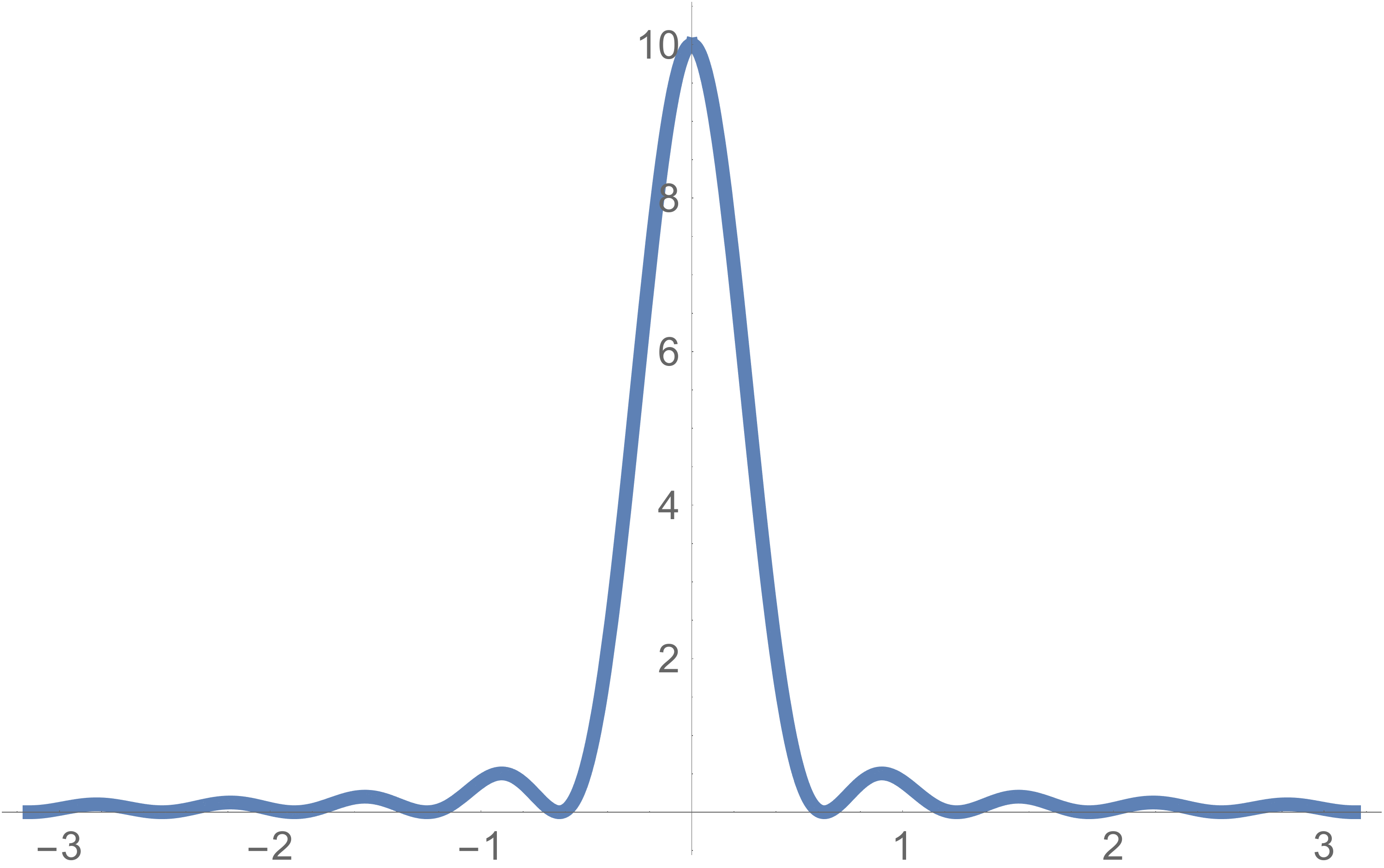
Figure 1. The Fejér kernel $F_{N}=\frac{1}{N}\frac{\sin^{2}(Nx/2)}{\sin^{2}(x/2)}$ for $N=10$.

Proposition 8.

The map $S_{n}:C(S^{1})^{(n)}\to C(S^{1})$ defined for any $T\in C(S^{1})^{(n)}$ by $S_{n}(T)(x)=\operatorname{Tr}\left(|\psi\rangle\langle\psi|\alpha_{x}(T)\right)$ satisfies

$$\langle f,S_{n}(T)\rangle_{L^{2}(S^{1})}=\frac{1}{n}\operatorname{Tr}\left((R_{n}(f))^{*}T\right).$$

Moreover, we may write

$$S_{n}(R_{n}(f))(x)=\sum_{k=-n+1}^{n-1}\left(1-\frac{|k|}{n}\right)a_{k}e^{ikx}=(F_{n}*f)(x)$$

in terms of the Fejér kernel $F_{n}$ and the Fourier coefficients $a_{k}$ of $f$.

Proof.

Let us first check the formula for $S_{n}(T)$ by computing that

$$\operatorname{Tr}\left(|\psi\rangle\langle\psi|\alpha_{x}(T)\right)=\frac{1}{n}\sum_{k,l}T_{kl}e^{i(k-l)x}=\frac{1}{n}\sum_{k=-n+1}^{n-1}(n-|k|)a_{k}e^{ikx}$$

Thus, $S_{n}(T)=F_{n}*f$ when $T=PfP$ —again understanding $f$ as an operator acting on $L^{2}(S^{1})$— and we may use elementary Fourier theory (cf. [30, Proposition 3.1(vi)])to derive

$$\langle g,S_{n}(T)\rangle =\langle g,F_{n}*f\rangle=\sum_{k=-n+1}^{n-1}\overline{b_{k}}a_{k}\left(1-\frac{|k|}{n}\right),$$

where $$b_{k} g$$ are the Fourier coefficients of . On the other hand, we have

$$\frac{1}{n}\operatorname{Tr}\left((R_{n}(g))^{*}T\right) =\frac{1}{n}\sum_{k,l=-n+1}^{n-1}\overline{b_{k-l}}a_{k-l}=\frac{1}{n}\sum_{k=-n+1}^{n-1}\overline{b_{k}}a_{k}\left(n-|k|\right).\qed$$

3.1.2. The circle as a limit of its spectral truncations

Let us now show in a series of Lemma’s that the conditions of Definition 2 are satisfied.

Lemma 9.

For any $f\in C^{\infty}(S^{1})$ we have $\|R_{n}(f)\|\leq\|f\|$ and $\|[D,R_{n}(f)]\|\leq\|[D,f]\|$.

Proof.

Since $R_{n}(f)=PfP$ and $P$ commutes with $D$ this follows directly since $P$ is a projection. ∎

Lemma 10.

There exists a sequence $\{\gamma_{n}\}$ converging to 0 such that

$$\|f-S_{n}(R_{n}(f))\|\leq\gamma_{n}\|[D,f]\|$$

for all $f\in C^{\infty}(S^{1})$.

Proof.

Since $\|[D,f]\|$ is equal to the Lipschitz constant for $f$ [8, Proposition 1] we have that $|f(x)-f(z)|\leq|x-z|\|[D,f]\|$. We use this in the following estimate

$$|f(x)-S_{n}(R_{n}(f))(x)| \leq\frac{1}{2\pi}\int_{-\pi}^{\pi}F_{n}(y)|f(x)-f(y-x)|dy$$

$$\leq\frac{1}{2\pi}\int_{-\pi}^{\pi}F_{n}(y)|y|dy\cdot\|[D,f]\|=:\gamma_{n}\|[D,f]\|.$$

Becasue the Fejér kernels form an approximate delta-function at $0$ (cf. [30, Theorem 4.1 and Lemma 5.1]) imply that $\gamma_{n}\to 0$. ∎

Lemma 11.

For any $T\in C(S^{1})^{(n)}$ we have $\|S_{n}(T)\|\leq\|T\|$ and $\|[D,S_{n}(T)]\|\leq\|[D,T]\|$.

Proof.

First note that $[D,S_{n}(T)]$ is a function on $S^{1}$ (it is $i$ times the derivative of $S_{n}(T)$). Moreover, we have

$$|[D,S_{n}(T)](x)| =|\operatorname{Tr}\left(|\psi\rangle\langle\psi|\alpha_{x}([D,T])\right)|\leq\||\psi\rangle\langle\psi|\|_{1}\|\alpha_{x}([D,T])\|\leq\|[D,T]\|.$$

Since this holds for any $x$, we may take the supremum to arrive at the desired inequality. The other inequality is even easier. ∎

Lemma 12.

There exists a sequence $\{\gamma_{n}^{\prime}\}$ converging to 0 such that

$$\|T-R_{n}(S_{n}(T))\|\leq\gamma^{\prime}_{n}\|[D,T]\|$$

for all $T\in C(S^{1})^{(n)}$.

Proof.

Write $T=PgP$ for $g=\sum_{k}b_{k}e^{ikx}$. Then the matrix coefficients of the Toeplitz matrix $T-R_{n}(S_{n}(T))$ are given by

$$(T_{kl}-R_{n}(S_{n}(T))_{kl}) =\begin{pmatrix}b_{k-l}\end{pmatrix}-\begin{pmatrix}1-\frac{|k-l|}{n}b_{k-l}\end{pmatrix}=\begin{pmatrix}\frac{|k-l|}{n}b_{k-l}\end{pmatrix}$$

$$=(T_{n}-T_{n}^{*})\odot\begin{pmatrix}\frac{k-l}{n}b_{k-l}\end{pmatrix}$$

$$=\frac{1}{n}(T_{n}-T_{n}^{*})\odot\begin{pmatrix}[D,T]\end{pmatrix}$$

in terms of the Schur product $\odot$ with $T_{n}$ and $T_{n}^{*}$ where

$$T_{n}=\begin{pmatrix}1&0&\cdots&0\\ 1&1&\cdots&0\\ \vdots&\vdots&\ddots&\vdots\\ 1&1&\cdots&1\end{pmatrix}.$$

Now the norm of the map $A\mapsto T_{n}\odot A$ for $A\in M_{n}(\mathbb{C})$ coincides with $\|T_{n}\|_{cb}$ (cf. [25, Chapter 8]). In [1, Theorem 1] the following estimate for this norm was derived:

$$\|T_{n}\|_{cb}\leq\left(1+\frac{1}{\pi}(1+\log(n))\right).$$

Hence we have

$$\|T-R_{n}(S_{n}(T))\| \leq\frac{2}{n}\|T_{n}\|_{cb}\|[D,T]\|\leq\gamma_{n}^{\prime}\|[D,T]\|$$

where $\gamma_{n}^{\prime}:=\frac{2}{n}\left(1+\frac{1}{\pi}(1+\log(n))\right)$. It is clear that $\gamma_{n}^{\prime}\to 0$ as $n\to\infty$. ∎

Thus we find that the pair of maps $(R_{n},S_{n})$ for $\{(C(S^{1})^{(n)},P_{n}L^{2}(S^{1}),P_{n}DP_{n})\}_{n}$ and $(C^{\infty}(S^{1}),L^{2}(S^{1}),D)$ forms a $C^{1}$-approximate order isomorphism. We may conclude from Theorem 5 that

Proposition 13.

The sequence of state spaces $\{(\mathcal{S}(C(S^{1})^{(n)}),d_{n})\}_{n}$ converges to $(\mathcal{S}(C(S^{1})),d)$ in Gromov–Hausdorff distance.

Using a simple Python script we have computed the distance function for states on $C(S^{1})^{(n)}$ of the form $S_{n}^{*}({\rm ev}_{x})$ for $n=3,5,9$, where ${\rm ev}_{x}$ is the pure state on $C(S^{1})$ given by evaluation at $x$. The optimization problem for computing the distance has been solved numerically using the standard sequential least squares programming (SLSQP) method and we claim absolutely no originality or proficiency here. We have illustrated the numerical results in Figure 2.

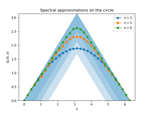
Figure 2. The distance function $d_{n}(0,x)\equiv d_{n}(0,S_{n}^{*}({\rm ev}_{x}))$ on the Toeplitz operator system (Proposition 13) for $n=3,5,9$. The blue band corresponds to the lower bounds $d(0,x)-2\gamma_{n}$ given in Proposition 4 with the constants $\gamma_{n}$ given in Lemma 10.

3.2. Fejér–Riesz operator systems converge to the circle

In [10] we found the dual operator system of $C(S^{1})^{(n)}$ to be equal to the operator system of functions on $S^{1}$ with only a finite number of non-zero Fourier coefficients. It gives a different type of truncation, this time taking place at the level of the function algebra, as opposed to a spectral truncation in Hilbert space.

More precisely, we will consider the so-called Fejér–Riesz operator system:

(4) $$C^{*}(\mathbb{Z})_{(n)}=\left\{a=(a_{k})_{k\in\mathbb{Z}}:\text{supp}(a)\subset(-n,n)\right\}.$$

The elements in $C^{*}(\mathbb{Z})_{(n)}$ are thus given by sequences with finite support of the form

$$a=(\ldots,0,a_{-n+1},a_{-n+2},\ldots,a_{-1},a_{0},a_{1},\ldots,a_{n-2},a_{n-1},0,\ldots)$$

and this allows to view $C^{*}(\mathbb{Z})_{(n)}$ as an operator subsystem of $C^{*}(\mathbb{Z})\cong C(S^{1})$.

The adjoint $a\mapsto a^{*}$ is given by $a^{*}_{k}=\overline{a}_{-k}$ and an element $a\in C^{*}(\mathbb{Z})_{(n)}$ is positive iff $\sum_{k}a_{k}e^{ikx}$ defines a positive function on $S^{1}$.

Since this naturally is an operator subsystem of $C(S^{1})$ it is natural to consider the following spectral triple:

(5) $$\left(C^{*}(\mathbb{Z})_{(n)},\mathcal{H}=L^{2}(S^{1}),D=-i\frac{d}{dx}\right).$$

We will be looking for positive and contractive maps $K_{n}:C(S^{1})\to C^{*}(\mathbb{Z})_{(n)}$ and $L_{n}:C^{*}(\mathbb{Z})_{(n)}\to C(S^{1})$ satisfying the conditions of Definition 2 so that we can apply Theorem 5 to conclude Gromov–Hausdorff convergence of the corresponding state spaces.

We introduce

$$K_{n}:C(S^{1}) \to C^{*}(\mathbb{Z})_{(n)}$$

$$f \mapsto F_{n}\ast f$$

where we recall that $$F_{n}=\sum_{|k|\leq n-1}(1-|k|/n)e^{ikx} K_{n} C^{*}(\mathbb{Z})_{(n)} C(S^{1}) L_{n} C^{*}(\mathbb{Z})_{(n)} C^{*}(\mathbb{Z})\cong C(S^{1})$$ is the Fejér kernel so that indeed maps to considered as an operator subsystem of . The map is simply the linear embedding of as an operator subsystem of :

$$L_{n}:C^{*}(\mathbb{Z})_{(n)} \to C(S^{1})$$

$$(a_{k}) \mapsto\left(x\mapsto\sum_{k}a_{k}e^{ikx}\right).$$

Positivity and contractiveness of $K_{n}$ for the norm and Lipschitz norm is an easy consequence of the good kernel properties of $F_{n}$ while for $L_{n}$ they are trivially satisfied.

Lemma 14.

There exists a sequence $\gamma_{n}$ converging to 0 such that

$$\|L_{n}\circ K_{n}(f)-f\|\leq\gamma_{n}\|[D,f]\|$$

for all $f\in C^{\infty}(S^{1})$.

Proof.

Since $L_{n}\circ K_{n}(f)=F_{n}\ast f$ the proof is analogous to that of Lemma 10. ∎

Lemma 15.

There exists a sequence $\gamma_{n}^{\prime}$ converging to 0 such that

$$\|K_{n}\circ L_{n}(a)-a\|\leq\gamma_{n}^{\prime}\|[D,a]\|$$

for all $a\in C^{*}(\mathbb{Z})_{(n)}$.

Proof.

From the Fourier coefficients of the Fejér kernel we find that

$$K_{n}\circ L_{n}(a)-a=\left(-\frac{|k|}{n}a_{k}\right)_{k}.$$

We will estimate the sup-norm of the function $f(x)=\frac{1}{n}\sum_{k}|k|a_{k}e^{ikx}$ by the Lipschitz norm of $a$. First of all, we may write $f$ as a convolution product $f=g\ast h$ where $g=\sum_{k=-n+1}^{n-1}\text{sgn}(k)e^{ikx}$ and $h=\frac{1}{n}\sum_{k=-n+1}^{n-1}ka_{k}e^{ikx}=\frac{1}{n}[D,a]$. Then $\|f\|_{\infty}\leq\|g\|_{1}\|h\|_{\infty}$ where

$$\|g\|_{1}\leq\|g\|_{2}=\sqrt{2n-1}.$$

We conclude that $\|g\ast h\|_{\infty}\leq\gamma^{\prime}_{n}\|[D,a]\|_{\infty}$ with $\gamma_{n}^{\prime}=\frac{\sqrt{2n-1}}{n}\to 0$ as $n\to\infty$. ∎

We conclude that the pair of maps $(K_{n},L_{n})$ for $\{(C^{*}(\mathbb{Z})_{(n)},L^{2}(S^{1}),D)\}_{n}$ and $(C^{\infty}(S^{1}),L^{2}(S^{1}),D)$ forms a $C^{1}$-approximate order isomorphism and we have

Proposition 16.

The sequence of state spaces $\{(\mathcal{S}(C^{*}(\mathbb{Z})_{(n)}),d_{n})\}_{n}$ converges to $(\mathcal{S}(C(S^{1})),d)$ in Gromov–Hausdorff distance.

We again illustrate the numerical results for the first few cases in Figure 3. As compared to the Toeplitz operator system (Figure 2) the optimization is much more cumbersome. This is essentially due to the fact that it involves the computation of a supremum norm of a trigonometric polynomial.

Remark 17.

If we recall the duality between $C(S^{1})^{(n)}$ and $C^{*}(\mathbb{Z})_{(n)}$ as operator systems from [10] it is quite surprising that both operator system spectral triples converge to the circle as $n\to\infty$.

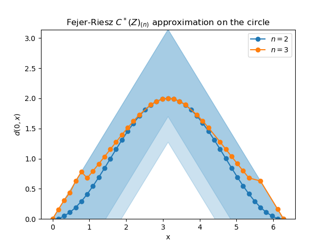
Figure 3. The distance function $d_{n}(0,x)\equiv d_{n}(0,L_{n}^{*}{\rm ev}_{x})$ on the Fejér–Riesz operator system (Proposition 16) for $n=2,3$. The blue band corresponds to the lower bounds $d(0,x)-2\gamma_{n}$ given in Proposition 4 with the constants $\gamma_{N}$ given in Lemma 14.

3.3. Matrix algebras converge to the sphere

In [28, 29] Rieffel analyzed quantum Gromov–Hausdorff convergence for so-called quantum metric spaces. Such a space is given by a pair $(A,L)$ of an order-unit space $A$ and a so-called Lipschitz norm $L$ on $A$. At first sight, such spaces appear to be more general than (operator system) spectral triples and the distance function they give rise to. However, as Rieffel shows in [28, Appendix 2] Dirac operators are universal in the sense that the Lipschitz semi-norms can always be realized as norms of commutators with a self-adjoint operator $D$. Note that it remains an open question, however, for what Lipschitz semi-norms one can find an operator $D$ with compact resolvent implementing that semi-norm.

We show below that the corresponding state spaces with Connes’ distance formula converge in Gromov–Hausdorff distance to the state space on the round two-sphere. This is closely connected —certainly at the technical level— to the results of [29] which is that the matrix algebras that describe the fuzzy two-sphere converge in quantum Gromov–Hausdorff distance to the round two-sphere. Even though for much of the analysis we may refer to [28, 29] we do formulate the main results in our framework of operator system spectral triples and, as said, restrict our attention to the classical metric spaces.

We will describe the round two-sphere by the following spectral triple:

(6) $$(C^{\infty}(S^{2}),\mathbb{C}^{2}\otimes L^{2}(S^{2}),D_{S^{2}})$$

We write $S^{2}=\{(x_{1},x_{2},x_{3})\in\mathbb{R}^{3}:x_{1}^{2}+x_{2}^{2}+x_{3}^{2}=1\}$ so that the following vector fields

$$X_{jk}=x_{j}\partial_{k}-x_{k}\partial_{j};\qquad(j<k).$$

are tangent to $S^{2}$. Of course, these vector fields are fundamental vector fields and generate the Lie algebra $su(2)$. Note that the normal vector field is given by $\vec{x}$ itself.

In terms of the three Pauli matrices we may then write the Dirac operator as [32]

(7) $$D_{S^{2}}=(\vec{x}\cdot\vec{\sigma})\sum_{j<k}\sigma^{j}\sigma^{k}\otimes X_{jk}.$$

Note that $(\vec{x}\cdot\vec{\sigma}):=\sum_{k=1}^{3}x_{k}\sigma_{k}$ acts as the chirality operator and makes sure that the spinor bundle on $S^{2}$ is actually non-trivial (as it should).

The fuzzy sphere [24] is obtained when one considers spherical harmonics on the sphere only up to some maximum total spin. More precisely, it is described by a matrix algebra $L(V_{n})$ where $V_{n}$ is the $n$-dimensional irreducible representation of $SU(2)$. A Dirac operator on the fuzzy sphere was introduced in [15] (see also [2]):

(8) $$D_{n}:=\sum_{j<k}\sigma^{j}\sigma^{k}\otimes[L_{jk},\cdot]$$

where $L_{jk}$ are standard generators of $su(2)$ in the $n$-dimensional representation, satisfying

$$[L_{jk},L_{lm}]=\delta_{kl}L_{jm}-\delta_{km}L_{jl}-\delta_{jl}L_{km}+\delta_{jm}L_{kl}.$$

This gives rise to the following spectral triple

(9) $$(L(V_{n}),\mathbb{C}^{2}\otimes L(V_{n}),D_{n})$$

The comparison between (7) and (8) is convincing, except for the absence of the chirality operator in the case of the fuzzy sphere. However, as shown in [2] this can be repaired for by a doubling of the representation space and a corresponding doubling constructing for the Dirac operator. Note that this does not alter the corrresponding Lipschitz norms, so we may just as well work with the Dirac operator defined in (8).

Remark 18.

The paper [2] also contains a detailed discussion on the nature of the spectral truncation that applies to the case at hand (see [2, Section 6.3]). It depends on the decomposition of the Hilbert space of spinors into irreducible representations of $\text{Spin}(3)$. However, since we will not need the specific form of the truncation here, we refrain from including it here.

Let us now proceed to show that there is a $C^{1}$-approximate order isomorphism $(\breve{\sigma},\sigma)$ for the sequence of spectral triples defined in (9) and the spectral triple of (6). As a consequence, we thus re-establish part of the conclusion of [29, Theorem 3.2] that the fuzzy sphere converges to the two-sphere in Gromov–Hausdorff distance as $n\to\infty$. Note that loc.cit. goes further in establishing that this limit is the unique limit of the sequence of fuzzy spheres (and also extends to more general coadjoint orbits). The reason we have included this example here is that it is formulated entirely in terms of spectral triples, and fits the general framework set up in Section 2.

3.3.1. Berezin symbol and Berezin quantization

Following [29] we start by defining maps $\sigma:L(V_{n})\to C(S^{2})$ and $\breve{\sigma}:C(S^{2})\to L(V_{n})$. Given a projection $P\in L(V_{n})$, say, on the highest-weight vector of $V_{n}$, we define the Berezin symbol $\sigma:L(V_{n})\to C(S^{2})$ by [5]

(10) $$\sigma(T)(g)\equiv\sigma_{T}(g):=\operatorname{Tr}(T\alpha_{g}(P))$$

where $\alpha_{g}$ is the action of $g\in SU(2)$ induced by conjugation on $L(V)$. Since $\alpha_{u}(P)=P$ for all $u\in U(1)$, it follows that $\sigma(T)$ is $U(1)$-invariant and thus descends to a function on $SU(2)/U(1)=S^{2}$. Moreover, we readily see that $\sigma$ is an $SU(2)$-equivariant map which will turn out to be useful later.

We let $\breve{\sigma}:C(S^{2})\to L(V_{n})$ be the adjoint of the map $\sigma$ when $C(S^{2})$ comes equipped with the $L^{2}$-inner product and $L(V_{n})$ with the Hilbert–Schmidt inner product. There is also the following explicit expression (cf. [29, Sect.2]).

Proposition 19.

The map $\breve{\sigma}$ defined by $\breve{\sigma}(f)\equiv\breve{\sigma}_{f}=n\int f(g)\alpha_{g}(P)dg$ satisfies

$$\langle f,\sigma_{T}\rangle=\frac{1}{n}\operatorname{Tr}(\breve{\sigma}_{f}T).$$

Moreover, we may write the so-called Berezin transform as a convolution product

$$\sigma(\breve{\sigma}_{f})(g)=(f\ast H_{P})(g)\equiv\int f(gh^{-1})H_{P}(h)dh$$

where $H_{P}$ is a probability measure defined by

$$H_{P}(g)=n\operatorname{Tr}(P\alpha_{g}(P)).$$

Proof.

As in [29, Sect.2] we check the formula for $\breve{\sigma}(f)$ by computing that

$$\langle f,\sigma_{T}\rangle=\int f(g)\operatorname{Tr}(T\alpha_{g}(P))dg=\operatorname{Tr}\left(\int f(g)T\alpha_{g}(P)dg\right)$$

so that the result follows.

For the Berezin transform we then indeed have that

$$\sigma(\breve{\sigma}_{f})(g) =\operatorname{Tr}\left(\breve{\sigma}_{f}\alpha_{x}(P)\right)=\operatorname{Tr}\left(n\int f(h)\alpha_{h}(P)dh\alpha_{g}(P)\right)$$

$$=n\int f(h)\operatorname{Tr}(P\alpha_{h^{-1}g}(P))dh=n\int f(gh^{-1})H_{P}(h)dh$$

using also that $H_{P}(h^{-1})=H_{P}(h)$. ∎

Again, one readily observes that $\breve{\sigma}$ is an $SU(2)$-equivariant map.

3.3.2. The sphere as a limit of matrix algebras

We now show in a series of Lemma’s that the conditions of Definition 2 hold for $R_{n}=\breve{\sigma}$ and $S_{n}=\sigma$.

Lemma 20.

For any $f\in C^{\infty}(S^{2})$ we have $\|\breve{\sigma}_{f}\|\leq\|f\|$ and $\|[D_{n},\breve{\sigma}_{f}]\|\leq\|[D_{S^{2}},f]\|$.

Proof.

The contractive property of $\breve{\sigma}$ is proved for instance in [19, Theorem 1.3.5] where $\breve{\sigma}$ is the Berezin quantization map. Then, by $SU(2)$-equivariance of $\breve{\sigma}$ we have

$$[D_{n},\breve{\sigma}_{f}]=\sum_{j<k}\sigma^{j}\sigma^{k}\otimes[L_{jk},\breve{\sigma}_{f}]=\left(\sum_{j<k}\sigma^{j}\sigma^{k}\otimes\breve{\sigma}([X_{jk},f])\right)=(1\otimes\breve{\sigma})[D_{S^{2}},f].$$

Since $\breve{\sigma}$ is a positive map from a commutative domain to a $C^{*}$-algebra, it follows by a Theorem by Stinespring [31] (cf. [25, Theorem 3.11]) that $\breve{\sigma}$ is completely positive. But then, it follows from [25, Proposition 3.6] that $\breve{\sigma}$ is completely bounded with $\|\breve{\sigma}\|_{cb}=\|\breve{\sigma}\|$. In particular, $\|1\otimes\breve{\sigma}\|\leq\|\breve{\sigma}\|\leq 1$ so that it follows that

$$\|[D_{n},\breve{\sigma}_{f}]\|\leq\|(1\otimes\breve{\sigma})\|\|[D_{S^{2}},f]\|\leq\|[D_{S^{2}},f]\|.\qed$$

Lemma 21.

There exists a sequence $\{\gamma_{n}\}$ converging to 0 such that

$$\|f-\sigma(\breve{\sigma}_{f})\|\leq\gamma_{n}\|[D_{S^{2}},f]\|$$

for all $f\in C^{\infty}(S^{2})$.

Proof.

We exploit the expression for $\sigma(\breve{\sigma}_{f})$ as a convolution product from Proposition 19. Indeed,

$$|f(g)-\sigma(\breve{\sigma}_{f})(g)| =\left|\int(f(g)-f(h))H_{P}(h^{-1}g)dh\right|$$

$$\leq\|f\|_{\text{Lip}}\int d(g,h)H_{P}(h^{-1}g)dh=\|f\|_{\text{Lip}}\int d(e,h)H_{P}(h)dh$$

where $d$ is the $SU(2)$-invariant (round) distance on $SU(2)/U(1)$ and $\|f\|_{\text{Lip}}$ is the corresponding Lipschitz seminorm of $f$. Since $\|f\|_{\text{Lip}}=\|[D_{S^{2}},f]\|$ by standard arguments [9, Sect. VI.1] and $\int d(e,h)H_{P}(h)dh\to 0$ as $n\to\infty$, the result follows. ∎

Lemma 22.

For any $T\in L(V_{n})$ we have $\|\sigma_{T}\|\leq\|T\|$ and $\|[D_{S^{2}},\sigma_{T}]\|\leq\|[D_{n},T]\|$.

Proof.

The map $\sigma$ is a contraction:

$$\|\sigma_{T}\|=\sup_{g}|\operatorname{Tr}T\alpha_{g}(P)|\leq\|T\|\sup_{g}\operatorname{Tr}|\alpha_{g}(P)|=\|T\|.$$

Since $\sigma$ is also $SU(2)$-equivariant we again find that

$$[D_{S^{2}},\sigma_{T}]=\sum_{j<k}\sigma^{j}\sigma^{k}\otimes[X_{jk},\sigma_{T}]=\left(\sum_{j<k}\sigma^{j}\sigma^{k}\otimes\sigma([L_{jk},T])\right)=(1\otimes\sigma)[D_{n},T].$$

Since the range of $\sigma$ is a commutative $C^{*}$-algebra it follows from [25, Theorem 3.9] that $\|\sigma\|_{cb}=\|\sigma\|$. Hence

$$\|[D_{S^{2}},\sigma_{T}]\|\leq\|(1\otimes\sigma)\|\|[D_{n},T]\|\leq\|[D_{n},T]\|$$

since $\sigma$ is a contraction. ∎

Lemma 23.

There exists a sequence $\{\gamma_{n}^{\prime}\}$ converging to 0 such that

$$\|T-\breve{\sigma}(\sigma_{T})\|\leq\gamma^{\prime}_{n}\|[D_{n},T]\|$$

for all $T\in L(V_{n})$.

Proof.

This is based on a highly non-trivial result [29, Theorem 6.1] which states that there exists a sequence $\{\gamma_{n}^{\prime}\}$ converging to 0 such that

$$\|T-\breve{\sigma}(\sigma_{T})\|\leq\gamma^{\prime}_{n}L_{n}(T)$$

for all $T\in L(V_{n})$, where $L_{n}$ is the Lipschitz norm on $L(V_{n})$ defined by

$$L_{n}(T)=\sup_{g\neq e}\frac{\|\alpha_{g}(T)-T\|}{l(g)}$$

for a length function $g$ on $SU(2)$ that induces the round metric on $S^{2}$. However, as in the proof of [26, Theorem 3.1] we may estimate

$$L_{n}(T)\leq\sup_{X\in su(2)}\{\|[X,T]\|:\|X\|\leq 1\}$$

while the right-hand side can be bounded from above by $k\|[D,T]\|$ for some constant $k$ independent of $n$ (as in the display preceding [26, Theorem 4.2]. ∎

We have thus verified that the maps $(\breve{\sigma},\sigma)$ between $\{L(V_{n}),\mathbb{C}^{2}\otimes L(V_{n}),D_{n})$ and $(C^{\infty}(S^{2}),\mathbb{C}^{2}\otimes L^{2}(S^{2}),D_{S^{2}})$ forms a $C^{1}$-approximate order isomorphism and we may conclude from Theorem 5 that

Proposition 24.

The sequence of state spaces $\{(\mathcal{S}(L(V_{n})),d_{n})\}_{n}$ converges in Gromov–Hausdorff distance to $(\mathcal{S}(C(S^{2})),d)$.

References

- [1] J. R. Angelos, C. C. Cowen, and S. K. Narayan. Triangular truncation and finding the norm of a Hadamard multiplier. Linear Algebra Appl. 170 (1992) 117–135.
- [2] J. W. Barrett. Matrix geometries and fuzzy spaces as finite spectral triples. J. Math. Phys. 56 (2015) 082301, 25.
- [3] J. W. Barrett and L. Glaser. Monte Carlo simulations of random non-commutative geometries. J. Phys. A49 (2016) 245001.
- [4] T. Berendschot. Truncated geometry. Master’s thesis, Radboud University Nijmegen, 2019.
- [5] F. A. Berezin. General concept of quantization. Comm. Math. Phys. 40 (1975) 153–174.
- [6] D. Burago, Y. Burago, and S. Ivanov. A course in metric geometry, volume 33 of Graduate Studies in Mathematics. American Mathematical Society, Providence, RI, 2001.
- [7] M. D. Choi and E. G. Effros. Injectivity and operator spaces. J. Functional Analysis 24 (1977) 156–209.
- [8] A. Connes. Compact metric spaces, Fredholm modules, and hyperfiniteness. Ergodic Theory Dynam. Systems 9 (1989) 207–220.
- [9] A. Connes. Noncommutative Geometry. Academic Press, San Diego, 1994.
- [10] A. Connes and W. van Suijlekom. Spectral truncations in noncommutative geometry and operator systems. To appear in Commun. Math. Phys. [arXiv:2004.14115].
- [11] F. D’Andrea, F. Lizzi, and P. Martinetti. Spectral geometry with a cut-off: topological and metric aspects. J. Geom. Phys. 82 (2014) 18–45.
- [12] F. D’Andrea, F. Lizzi, and J. C. Várilly. Metric properties of the fuzzy sphere. Lett. Math. Phys. 103 (2013) 183–205.
- [13] L. Glaser and A. Stern. Reconstructing manifolds from truncated spectral triples. arXiv:1912.09227.
- [14] L. Glaser and A. Stern. Understanding truncated non-commutative geometries through computer simulations. J. Math. Phys. 61 (2020) 033507.
- [15] H. Grosse and P. Prešnajder. The Dirac operator on the fuzzy sphere. Lett. Math. Phys. 33 (1995) 171–181.
- [16] J. Kaad. Exterior products of compact quantum metric spaces. (work in progress).
- [17] D. Kerr. Matricial quantum Gromov-Hausdorff distance. J. Funct. Anal. 205 (2003) 132–167.
- [18] D. Kerr and H. Li. On Gromov-Hausdorff convergence for operator metric spaces. J. Operator Theory 62 (2009) 83–109.
- [19] N. P. Landsman. Mathematical Topics between Classical and Quantum Mechanics. Springer, New York, 1998.
- [20] F. Latrémolière. Convergence of fuzzy tori and quantum tori for the quantum Gromov-Hausdorff propinquity: an explicit approach. Münster J. Math. 8 (2015) 57–98.
- [21] F. Latrémolière. The dual Gromov-Hausdorff propinquity. J. Math. Pures Appl. (9) 103 (2015) 303–351.
- [22] F. Latrémolière. The quantum Gromov-Hausdorff propinquity. Trans. Amer. Math. Soc. 368 (2016) 365–411.
- [23] F. Latrémolière. Quantum metric spaces and the Gromov-Hausdorff propinquity. In Noncommutative geometry and optimal transport, volume 676 of Contemp. Math., pages 47–133. Amer. Math. Soc., Providence, RI, 2016.
- [24] J. Madore. The fuzzy sphere. Classical Quantum Gravity 9 (1992) 69–87.
- [25] V. Paulsen. Completely bounded maps and operator algebras, volume 78 of Cambridge Studies in Advanced Mathematics. Cambridge University Press, Cambridge, 2002.
- [26] M. A. Rieffel. Metrics on states from actions of compact groups. Doc. Math. 3 (1998) 215–229.
- [27] M. A. Rieffel. Metrics on state spaces. Doc. Math. 4 (1999) 559–600.
- [28] M. A. Rieffel. Gromov-Hausdorff distance for quantum metric spaces. Mem. Amer. Math. Soc. 168 (2004) 1–65.
- [29] M. A. Rieffel. Matrix algebras converge to the sphere for quantum Gromov-Hausdorff distance. Mem. Amer. Math. Soc. 168 (2004) 67–91.
- [30] E. M. Stein and R. Shakarchi. Fourier analysis, volume 1 of Princeton Lectures in Analysis. Princeton University Press, Princeton, NJ, 2003. An introduction.
- [31] W. F. Stinespring. Positive functions on -algebras. Proc. Amer. Math. Soc. 6 (1955) 211–216.
- [32] A. Trautman. Spinors and the Dirac operator on hypersurfaces. I. General theory. J. Math. Phys. 33 (1992) 4011–4019.