Fast second-order implicit difference schemes for time distributed-order and Riesz space fractional diffusion-wave equations
Abstract
In this paper, fast numerical methods are established for solving a class of time distributed-order and Riesz space fractional diffusion-wave equations. We derive new difference schemes by the weighted and shifted Grnwald formula in time and the fractional centered difference formula in space. The unconditional stability and second-order convergence in time, space and distributed-order of the difference schemes are analyzed. In the one-dimensional case, the Gohberg-Semencul formula utilizing the preconditioned Krylov subspace method is developed to solve the symmetric positive definite Toeplitz linear systems derived from the proposed difference scheme. In the two-dimensional case, we also design a global preconditioned conjugate gradient method with a truncated preconditioner to solve the discretized Sylvester matrix equations. We prove that the spectrums of the preconditioned matrices in both cases are clustered around one, such that the proposed numerical methods with preconditioners converge very quickly. Some numerical experiments are carried out to demonstrate the effectiveness of the proposed difference schemes and show that the performances of the proposed fast solution algorithms are better than other numerical methods.
Keywords: Distributed-order diffusion-wave equation; Riesz fractional derivative; Toeplitz matrix; Gohberg-Semencul formula; Circulant preconditioner; Krylov subspace method;
1 Introduction
In recent years, fractional diffusion equations (FDEs) have gained more and more attention since their widespread applications in modeling complex processes such as finance [1], biology [2], chaos [3], optimal control [4], signal processing[5] and random walk [6]. In general, these models are constructed in the form of single or multi-term time, space or time-space FDEs. However, when the processes lack temporal scaling, neither single nor multi-term FDEs can describe them. Therefore distributed-order FDEs are introduced to model the processes that become more anomalous in course of time, e.g. the ultraslow diffusion or accelerating superdiffusion where a plume of particles spreads at a logarithmic rate [7, 8].
The idea of distributed-order FDEs was first introduced by Caputo [9] to generalize the stress-strain relations of unelastic media. In [10], Gorenflo et al. developed the fundamental solution for a 1D distributed-order fractional diffusion-wave equation by using the Fourier-Laplace transform and the interpolation technique. Li et al. [11] discussed an initial-boundary value problem of a time distributed-order FDE with the Caputo fractional derivative, where the analytical solution in time was obtained. However, the analytical solutions of many distributed-order FDEs are not easy to gain and the uniqueness and existence of the analytical solutions are not easy to prove. Therefore, different numerical methods for solving the distributed-order FDEs are considered.
Ye et al. [12] derived a compact difference scheme of a distributed-order fractional diffusion-wave system and demonstrated the unconditional stability and convergence of the difference scheme. A new numerical method based upon hybrid functions approximation was proposed by Mashayekhi et al. [13] to solve the distributed-order FDEs, which consists of Bernoulli polynomials and block-pulse functions. Bu et al. [14] developed a numerical scheme to solve distributed-order time FDEs with the finite element method in the space direction and the L1 method in the time direction. Then also gave the analysis of unconditional convergence and stability of the numerical method. In [15], Li et al. studied Galerkin finite element methods with non-uniform temporal meshes for multi-term Caputo-type FDEs, and proved that the corresponding finite element schemes were unconditionally convergent and stable. Gao et al. [16] constructed two difference schemes to solve 1D time distributed-order fractional wave equations and derived them from a weighted and shifted Grnwald formula with second-order accuracy.
However, the current research is still sparse about the numerical methods of distributed-order FDEs. This motivates us to develop efficient numerical solutions for the following time distributed-order and Riesz space fractional diffusion-wave equations:
| (1.1) | ||||
| (1.2) | ||||
| (1.3) |
where , , and is the source term. Here, is the Caputo fractional derivative [12] defined as:
and the weight function satisfies the conditions
Moreover, the right-side is the Riesz fractional derivative of order , whose definition is given by [17]
with denoting the Gamma function.
To establish the high-order accurate numerical method to solve the problem (1.1)-(1.3), we first transform Eqs. (1.1)-(1.3) into multi-term time-space diffusion-wave equations via the composite trapezoid formula [18]. Then by applying the weighted and shifted Grnwald formula [16] to discrete the time-fractional derivatives of the resulted multi-term equations, the second-order accurate approximation in time can be achieved. In addition, to gain the second-order accuracy in space, the fractional centered difference formula [19] is used to approximate the Riesz derivative. Hence, a new second-order difference scheme in all variables is developed.
When the above discrete methods are used to approximate the problem (1.1)-(1.3), the real symmetric positive definite (SPD) Toeplitz linear systems will be obtained. Because of the nonlocal characteristics [20] of the fractional derivative, the coefficient matrices are usually dense or even full. If the traditional methods like Cholesky factorization are used to solve the linear systems, the costs are significantly expensive, which require storage and computational work, where is the number of grid points. Since the coefficient matrix contains the Toeplitz structure, Krylov subspace methods (KSMs) are considered to solve the linear systems. Because KSMs only need the information of matrix-vector product that can be done in only operations via the fast Fourier transform (FFT) and the storage requirement is only [21, 22]. Various KSMs for the Toeplitz linear systems have been developed and studied [23, 24, 25].
Since the coefficient matrix has a SPD Toeplitz structure, its inverse matrix can be explicitly expressed by the Gohberg-Semencul formula (GSF)[26]. On the other hand, the coefficient matrix is also time-independent. Thus its inverse can be calculated only once and the cost for computing the inverse matrix-vector multiplication only needs four FFTs. In this work, the conjugate gradient (CG) method [23] is employed to solve the SPD Toeplitz linear system arising from the GSF. However, the CG method converges slowly when the coefficient matrix is ill-conditioned. To accelerate its convergence, some preconditioners [27, 28, 29, 30] are designed according to the structures of the the coefficient matrices.
In the 2D case, the GSF cannot be used since the coefficient matrix is a block Toeplitz with Toeplitz blocks (BTTB) matrix and not a Toeplitz matrix. Therefore, a new method needs to be designed to solve the resulting Sylvester matrix equations. In [31], S. Karimi presented a global CG (GL-CG) method for solving a large Sylvester matrix equation, and demonstrated that it was more effective than the CG method to deal with the corresponding Kronecker equation. In order to improve the convergence, we propose a global preconditioned CG (GL-PCG) method with a preconditioner to solve the Sylvester matrix equations. Moreover, it is well-known that a block circulant with circulant blocks (BCCB) [32] preconditioner of a BTTB matrix cannot be optimal, and a BTTB preconditioner of a BTTB matrix is optimal even if the eigenvalues of the preconditioner do not closely approximate the eigenvalues of the coefficient matrix [33]. Therefore, in this paper, we design a truncated preconditioner which has the same structure as the coefficient matrix to solve the 2D problem.
This paper has two goals: (1) to propose unconditionally stable difference schemes with second-order accuracy in time, space and distributed-order to solve the 1D and 2D problems; (2) to explore efficient algorithms for solving the resulted linear systems. In the 1D case, based on the SPD Toeplitz structure, the GSF utilizing the preconditioned KSM (referred to as PKSM-based GSF) is developed to process the linear systems, whose computational cost per iteration is only . Since the PKSM-based GSF cannot be directly applied to solve the 2D problem, we design the GL-PCG method with a truncated preconditioner to solve the discretized Sylvester matrix equations. It will be demonstrated that the spectrums of the preconditioned matrices are clustered around one. Therefore, the proposed numerical methods with preconditioners converge very quickly.
The outline of this paper is as follows. In Section 2, we introduce the derivation of the new difference scheme for the problem -. The unique solvability, unconditional stability, and second-order convergence of the difference scheme are proved in Section 3. In Section 4, the PKSM-based GSF is presented to solve the resulted SPD Toeplitz linear systems. The spectral properties of the preconditioned matrix are discussed in Section 5. In Section 6, the GL-PCG method with a truncated preconditioner is designed to handle the 2D problem. In Section 7, numerical experiments are provided to verify the second-order convergence of the difference schemes and show the efficiency of the proposed fast solution techniques. Finally, concluding remarks are given in Section 8.
2 The derivation of the difference scheme
In this section, we focus on deriving the new difference scheme of the problem -.
For , let and be the spatial grid size and time step, respectively. Then we can define and . The domain is covered by , where and . Let be a grid function on and define
Then the following lemmas are needed to derive the difference scheme.
Lemma 2.1.
Lemma 2.2.
[19] Suppose that satisfy the boundary condition . The fractional centered difference formula for approximating the Riesz derivatives when is as follows:
where
Consider at point :
| (2.1) |
Take an average of on time levels and to get
| (2.2) |
where .
Define on . Equation can be expressed as
| (2.3) |
Firstly, we consider the discretization of the integral term in . Let and suppose that , and . According to Lemma 2.1, we can obtain
where . Thus the problem is now transformed into the following multi-term fractional diffusion-wave equation:
| (2.4) |
Next, we introduce a difference scheme to solve the multi-term system with the initial-boundary conditions -. Suppose . For , using a fully discrete difference scheme in [16] and noticing the zero initial condition , we arrive at
| (2.5) |
where , and
| (2.6) |
with
In the meantime, using the Lemma 2.2 for approximating the Riesz derivatives in , we get
| (2.7) |
By substituting and into , we obtain
| (2.8) |
where , .
In addition, according to the initial and boundary value conditions, we obtain
| (2.9) | |||
| (2.10) |
Let be the numerical approximation to . Ignoring the error term in , we can derive the following difference scheme for -
| (2.11) | |||
| (2.12) | |||
| (2.13) |
Let and . Then the numerical scheme (2) can be rewritten into the following matrix form
| (2.14) |
in which
| (2.15) |
and
where is the identity matrix of order and ,
and
| (2.16) |
Note that has a Toeplitz structure [34]. According to Lemma 3.1 in Section 3, the matrix is also symmetric. Therefore, it can be stored with only entries and the Toeplitz matrix-vector product can be performed within operations using FFTs [35].
3 Solvability, stability and convergence analysis
In this section, we discuss the solvability, stability and convergence of the difference scheme (2)-(2.13). Before analyzing these properties, we first need to give some auxiliary definitions and useful lemmas as follows.
Denote the grid function space on by
For any , the discrete inner product and the corresponding discrete -norm are defined as follows:
According to Lemma 3.1, we get the following results.
Lemma 3.4.
Let . For any grid function , we have
where is a SPD matrix and satisfies .
Proof.
According to Lemma 3.1, it is easy to see that the is a SPD matrix, so is also SPD. Thus there is a SPD matrix such that , and we have
which completes the proof. ∎
Lemma 3.5.
Proof.
According to [37, Lemma 3.3], we can easily get that .
Then we prove that . Consider the 2-norm of given vector,
where is a orthogonal transformation, and are the eigenvalues of the matrix related to .
Thus, we get
So we just need to prove that . Using Lemma 3.1, we can easily get that the is a strictly diagonally dominant -matrix. According to [38, Theorem 1.1], and noticing Lemma 3.1, we have
The proof is completed. ∎
3.1 Solvability
3.2 Stability
In this subsection, we work towards proving the unconditional stability of the proposed difference scheme (2)-(2.13).
Theorem 3.2.
Let be the solution of the following difference system
| (3.1) | |||
| (3.2) | |||
| (3.3) |
Then it holds that
where and
Proof.
Taking the inner product of (3.2) with , we get
Using Lemma 3.4, we get
Summing up the above equality for from 1 to , we have
According to Lemma 3.3, we obtain
Consequently, we can get
where Lemma 3.5 applies to the last step. Then
Applying the Gronwall inequality [39, Lemma 2] for above equation, we obtain
Then by Lemma 3.5, it arrives at
The proof completed. ∎
3.3 Convergence
Now, we consider the convergence of the proposed difference scheme (2)-(2.13). The following theorem verifies the second-order accuracy of our proposed difference scheme in time, space and distributed order.
Theorem 3.3.
4 PKSM-based GSF
In this section, the implementation of the numerical method (2.14) is analyzed. Based on the SPD Toeplitz structure of the coefficient matrix, we will design the GSF utilizing the preconditioned CG (PCG-based GSF) method with a circulant preconditioner to solve the linear system (2.14).
In general, the implementation of the linear system (2.14) can be represented by the following algorithm.
In Algorithm 1, by exploiting the Toeplitz structure of the matrix , the matrix-vector product in Step 2 can be done in operations by FFTs. Since the coefficient matrix is time-independent (it does not depend on ), the solutions of (2.14) in Step 3 can be written as ) and can be calculated at the cost of one Cholesky factorization. However, the method requires considerable cost when is large and dense. Fortunately, has a SPD Toeplitz structure, so can be directly calculated by GSF [26, 40, 41] with limited memory and computational cost. More precisely, let = be the solution of the linear system
| (4.1) |
Then the matrix-vector multiplication by the GSF is formulated as
where is a dimensional anti-identity matrix, and represent the real and imaginary parts of , respectively, and
| (4.2) |
with and are lower Toeplitz matrices which are defined as
respectively.
We note that in (4.2), is a circulant matrix [27] and is a skew-circulant [42] matrix. Therefore, the cost of computing the is almost the same as computing one circulant and one skew-circulant matrix-vector product, or roughly only four -length FFTs with complexity. The algorithm to compute the product via GSF is given in Algorithm 2 as follows:
In summary, once the in (4.1) is obtained, the matrix-vector product can be done in operations with Algorithm 2. Next, an efficient iterative algorithm will be developed to solve the SPD Toeplitz linear system (4.1).
It is well-known that the CG method [23] is a popular and effective KSM for solving the SPD linear systems. However, the CG method usually converges slowly when the coefficient matrix is ill-conditioned or large. Therefore, the preconditioned CG (PCG) method is proposed to solve the linear system (4.1), whose computational complexity at each time step is only .
Now, a circulant preconditioner, which is generated from the R. Chan’s [21] preconditioner, is proposed to solve the linear system (4.1). Note that other circulant approximations, such as the Strang’s preconditioner [34], are also available but will not be discussed here. For a Toeplitz matrix defined as in (2.16), the R. chan’s preconditioner is a circulant matrix obtained by using all entries of [34]. More precisely, its entries are given by
Then, solving (4.1) is equivalent to solving the following preconditioned system
where the R. Chan’s-based circulant preconditioner is defined as
| (4.3) |
More precisely, the first column of is given by
.
To analyze the properties of the preconditioner , we first prove the following lemma.
Lemma 4.1.
For , the circulant matrix is real SPD, and all its eigenvalues fall inside .
Proof.
Then we can conclude that has the following properties.
Theorem 4.1.
For , the circulant preconditioner in (4.3) is SPD and
Proof.
By Lemma 4.1 and noting that , and , the circulant preconditioner is also a SPD matrix.
Suppose that are the eigenvalues of . According to Lemma 4.1, we have for each . Since the -th eigenvalue of is
we get for all . Furthermore, we have
and
which completes the proof. ∎
This theorem will be applied to prove the superlinear convergence rate of PCG method with R. Chan’s circulant preconditioner in the next section.
5 Spectrum of the preconditioned matrix
In this section, the spectral properties of the preconditioned matrix are analyzed. The eigenvalue distribution of the preconditioned matrix is one of the key factors that affect the convergence rate of the KSMs [21]. Usually, the convergence speed is fast if the spectrum of the preconditioned matrix is away from zero, and the preconditioned matrix can be expressed as the sum of an identity matrix, a matrix with small norm, and a matrix with low rank, especially for those matrices close to normal [22, 43]. For convenience, we choose proper , depending on , and find a such that
| (5.1) |
for all .
By the definition of generating function [34, pp.12-20], we can obtain that the generating function of is
We remark that the cannot be a generating function of in (2.15) since is dependent on . In order to prove the superlinear convergence of the preconditioned matrix , the following two lemmas are needed.
Lemma 5.1.
Let be the generating function of , then we get that the is in the Wiener class.
Lemma 5.2.
[44] If , the generating function of , is in the Wiener class, then for any , there exist and , such that for all , we have
where and .
Theorem 5.1.
If and , for any , there exist and such that, for any ,we have
where and .
Proof.
From Theorem 5.1, it holds that the preconditioned matrix is the sum of an identity matrix, a matrix with small norm, and a matrix with low rank. Thus the spectrum of is clustered around 1. Furthermore, since is clearly satisfied, and according to the Theorem 4.1 and Eq. (5.1), the smallest singular value of the matrix is
which implies is uniformly bounded away from zero. According to the Corollary 1.11 in [34], the superlinear convergence of the PCG method with R. Chan’s circulant preconditioner is obtained.
6 2D problem
In this section, we consider the following 2D problem:
| (6.1) | ||||
| (6.2) | ||||
| (6.3) | ||||
where , , , is the boundary of , and is a given function.
6.1 The derivation of the difference scheme
The numerical discrete methods applied to the 1D problem (1.1)-(1.3) can be directly extended to deal with the 2D problem (6.1)-(6.3).
To derive the difference scheme of (6.1)-(6.3), we first divide the interval into -subintervals with and , and divide the interval into -subintervals with and .
Let , , . Suppose and consider Eq. (6.1) at the point , we have
where . Taking an average of the above equality on time levels and , it follows
| (6.4) |
Let , then Eq. (6.4) can be expressed as
| (6.5) |
Using Lemma 2.1, we get
| (6.6) |
According to the fully discrete difference scheme in [16] and noticing the zero initial condition , we have
| (6.7) |
By substituting - into , we have
| (6.10) |
where , .
Omitting the small term in (6.10), replacing with its numerical one and noticing the initial and boundary value conditions (6.2)-(6.3), we can construct the numerical scheme of - as follows:
| (6.11) | |||
| (6.12) | |||
| (6.13) |
Similar to the Section 3, the difference scheme (6.11)-(6.13) can be proved to be uniquely solvable, unconditionally stable and convergent with the order of .
Let
The following matrix form for difference scheme (6.11) can get
| (6.14) |
where
| (6.15) |
and
in which denotes the Kronecker product, , and are identity matrices of order , and , respectively, and the definitions of and are similar to and , respectively.
6.2 GL-PCG method with truncated preconditioner
We remark that the PCG-based GSF method cannot be directly applied to handle the linear systems (6.14) since is a BTTB matrix and not a Toeplitz matrix. Therefore, in this subsection, we seek other effective algorithms to efficiently solve linear systems (6.14).
Let and . It is easy to verify that the Kronecker equations (6.14) are equivalent to the following Sylvester matrix equations
| (6.16) |
where
Proposition 6.1.
Let be a linear operator as follows:
Then the linear operator is SPD.
Proof.
The proof can be referred to the conclusion in [31, Proposition 1]. ∎
Since is SPD, the GL-CG method [31] is a good choice for solving the Sylvester matrix equations (6.16). However, the GL-CG method usually converges very slowly because the resulting matrix equations are often ill-conditioned. Therefore, we will develop the preconditioned GL-CG (GL-PCG) method to accelerate the convergence rate. More specifically, the GL-CG method is employed to solve its equivalent preconditioned linear matrix equation
where is a preconditioner operator. The algorithm of the GL-PCG method is given as follows.
In Step 5 of the GL-GCG algorithm, the inner product is defined as
where is the -th column of .
According to the well-known fact that a preconditioner with the same structure of the preconditioned matrix is optimal [33]. We now design a truncated preconditioner which has the same structure of as follows:
| (6.17) |
where is a -truncation for matrix (). More precisely,
The invertibility of is guaranteed by the following lemma.
Lemma 6.1.
For , the preconditioner operator is SPD.
Proof.
The truncated preconditioner can be expressed in the following Kronecker form
It is easy to prove that is SPD. From [31, Proposition 2], we get that is also SPD. ∎
We investigate numerically the eigenvalue distributions of the proposed preconditioned matrix , where (see Figs. 6-7). It is obvious that the spectrum of the preconditioned matrix is clustered around 1.
Two major computational loads in Algorithm 3 are and . The can be calculated by solving the Sylvester equation . Moreover, we observe that
which implies that the computation of includes two Toeplitz matrix multiplications, and . Therefore, it can be obtained by FFT2 with only .

(a) = 1.3 (b) = 1.8
7 Numerical results
Some numerical experiments are carried out in this section to verify the effectiveness of the proposed difference schemes and the performances of the fast solution techniques. All numerical experiments are implemented using MATLAB R2016a on a desktop with 16GB RAM, Inter (R) Core (TM) i7-8700K CPU @3.70GHz.
| 16 | 1.444281e-04 | - | 2.611489e-04 | - | 3.877349e-04 | - |
|---|---|---|---|---|---|---|
| 32 | 3.661426e-05 | 1.9799 | 6.585700e-05 | 1.9875 | 9.793241e-05 | 1.9852 |
| 64 | 9.261868e-06 | 1.9830 | 1.669595e-05 | 1.9798 | 2.469879e-05 | 1.9873 |
| 128 | 2.316352e-06 | 1.9994 | 4.176866e-06 | 1.9990 | 6.183403e-06 | 1.9980 |
| 256 | 5.812125e-07 | 1.9947 | 1.045642e-06 | 1.9980 | 1.547730e-06 | 1.9982 |
| 16 | 4.790434e-04 | - | 3.999822e-04 | - | 3.172525e-04 | - |
|---|---|---|---|---|---|---|
| 32 | 1.215018e-04 | 1.9792 | 1.013382e-04 | 1.9808 | 8.009703e-05 | 1.9858 |
| 64 | 3.058415e-05 | 1.9901 | 2.549518e-05 | 1.9909 | 2.011908e-05 | 1.9932 |
| 128 | 7.668025e-06 | 1.9959 | 6.393357e-06 | 1.9956 | 5.045536e-06 | 1.9955 |
| 256 | 1.915933e-06 | 2.0008 | 1.600711e-06 | 1.9979 | 1.267602e-06 | 1.9929 |
| 1 | 1.056413e-04 | - | 8.938958e-05 | - | 7.216282e-05 | - |
|---|---|---|---|---|---|---|
| 2 | 2.703158e-05 | 1.9665 | 2.288894e-05 | 1.9655 | 1.850067e-05 | 1.9637 |
| 4 | 6.789749e-06 | 1.9932 | 5.748842e-06 | 1.9933 | 4.646376e-06 | 1.9934 |
| 8 | 1.692476e-06 | 2.0042 | 1.431730e-06 | 2.0055 | 1.155441e-06 | 2.0077 |
| 16 | 4.158579e-07 | 2.0250 | 3.504514e-07 | 2.0305 | 2.810033e-07 | 2.0398 |
| PCG-GSF(R) | PCG-GSF(S) | |||||||||
|---|---|---|---|---|---|---|---|---|---|---|
| CPU | CPU(Iter) | Speed-up | CPU(Iter) | Speed-up | CPU | Speed-up | CPU | Speed-up | ||
| 0.01 | 0.02(4) | 0.50 | 0.02(4) | 0.50 | 0.02 | 0.50 | 0.02 | 0.50 | ||
| 0.07 | 0.06(4) | 1.17 | 0.06(4) | 1.17 | 0.05 | 1.40 | 0.05 | 1.40 | ||
| 0.25 | 0.21(4) | 1.19 | 0.22(4) | 1.14 | 0.20 | 1.25 | 0.20 | 1.25 | ||
| 1.2 | 1.19 | 0.84(4) | 1.42 | 0.84(4) | 1.42 | 0.73 | 1.63 | 0.73 | 1.63 | |
| 6.44 | 1.87(3) | 3.44 | 1.86(3) | 3.46 | 1.69 | 3.81 | 1.69 | 3.81 | ||
| 50.15 | 10.08(3) | 4.98 | 10.11(3) | 4.96 | 8.83 | 5.68 | 8.84 | 5.67 | ||
| 0.01 | 0.02(5) | 0.50 | 0.02(4) | 0.50 | 0.02 | 0.50 | 0.02 | 0.50 | ||
| 0.07 | 0.06(5) | 1.17 | 0.06(4) | 1.17 | 0.05 | 1.40 | 0.05 | 1.40 | ||
| 0.25 | 0.22(4) | 1.14 | 0.22(4) | 1.14 | 0.20 | 1.25 | 0.20 | 1.25 | ||
| 1.5 | 1.20 | 0.84(4) | 1.43 | 0.84(4) | 1.43 | 0.73 | 1.64 | 0.73 | 1.64 | |
| 6.51 | 1.98(4) | 3.29 | 1.97(4) | 3.30 | 1.69 | 3.85 | 1.69 | 3.85 | ||
| 50.12 | 10.78(4) | 4.65 | 10.79(4) | 4.65 | 8.85 | 5.66 | 8.85 | 5.66 | ||
| 0.01 | 0.02(5) | 0.50 | 0.02(5) | 0.50 | 0.02 | 0.50 | 0.02 | 0.05 | ||
| 0.07 | 0.06(5) | 1.17 | 0.06(5) | 1.17 | 0.05 | 1.40 | 0.05 | 1.40 | ||
| 0.25 | 0.22(5) | 1.14 | 0.22(5) | 1.14 | 0.20 | 1.25 | 0.20 | 1.25 | ||
| 1.9 | 1.17 | 0.84(4) | 1.39 | 0.84(4) | 1.39 | 0.73 | 1.60 | 0.73 | 1.60 | |
| 6.45 | 1.98(4) | 3.26 | 1.97(4) | 3.27 | 1.69 | 3.82 | 1.69 | 3.82 | ||
| 49.95 | 10.76(4) | 4.64 | 10.78(4) | 4.63 | 8.86 | 5.64 | 8.86 | 5.64 | ||
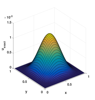
Example 7.1.
We first consider the 1D distributed-order and Riesz space fractional diffusion-wave problem:
with
where , and
The exact solution of the above problem is .
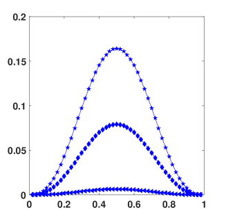
Gorenflo et al. [10] proposed that the solution of the distributed order time-fractional diffusion-wave problem can be interpreted as a probability density function of the spatial variable evolving in time . If we set , it reduces to the single order time-fractional diffusion-wave equation [45]. When , it becomes the time-fractional telegraph equation[46]. The probability density function is expressed through the weight function [8]. We chose in our experiment as in the references [14, 16, 18], which is advantageous to the exact solution is deduced.
To verify the convergence order of the proposed scheme (2)-(2.13), in Tables 1-3, let
where and are the exact and numerical solutions at step sizes , and , respectively. Thus the convergence orders are defined as
Tables 4-6 are to verify the efficiency of the proposed PCG-based GSF method described in Section 4. The resultant linear systems (2.14) of the 1D case are solved by using the Cholesky method, the PCG method and the proposed PCG-based GSF method, respectively. The stopping criterion of all iterative methods is
where is the residual vector after iterations, and the initial guess in each time level is given as the zero vector.
Besides the modified R. Chan’s preconditioner , we also test the Strang’s circulant preconditioner [47]:
where is the Strang’s circulant preconditioner for an arbitrary Toeplitz matrix. We can also prove that the preconditioner has similar theoretical properties to the preconditioner in the same way.
(a) =1.5 (b) = 5
In all tables, all times are the average of 10 runs of the algorithm. “CPU” stands for the total CPU time in seconds to solve the whole linear systems. “Chol” means that the Cholesky method is used to solve the discretized linear systems; “PCG(R)” means that the PCG method with R. Chan’s preconditioner is applied to solve the discretized linear systems; “PCG-GSF(R)” means that the proposed PCG-based GSF method with R. Chan’s preconditioner is applied to solve the discretized linear systems; The meanings of “PCG(S)” and “PCG-GSF(S)” are similar to “PCG(R)” and ‘PCG-GSF(R)”, respectively. In addition, “Speed-up” denotes the run time speed-up compared to the Cholesky method, e.g.:
Speed-up.
“Iter” means the average number of iterations of the method for solving the discretized linear systems at all time levels, i.e.,
where is the number of iterations at -th time step.
| PCG-GSF(R) | PCG-GSF(S) | |||||||||
|---|---|---|---|---|---|---|---|---|---|---|
| CPU | CPU(Iter) | Speed-up | CPU(Iter) | Speed-up | CPU | Speed-up | CPU | Speed-up | ||
| 0.01 | 0.02(4) | 0.50 | 0.02(4) | 0.50 | 0.02 | 0.50 | 0.02 | 0.50 | ||
| 0.07 | 0.06(4) | 1.17 | 0.06(4) | 1.17 | 0.05 | 1.40 | 0.05 | 1.40 | ||
| 0.25 | 0.22(4) | 1.14 | 0.22(4) | 1.14 | 0.20 | 1.25 | 0.20 | 1.25 | ||
| 1.2 | 1.20 | 0.84(4) | 1.43 | 0.83(4) | 1.45 | 0.72 | 1.67 | 0.72 | 1.67 | |
| 6.49 | 1.87(3) | 3.47 | 1.84(3) | 3.53 | 1.67 | 3.89 | 1.67 | 3.89 | ||
| 50.93 | 10.16(3) | 5.01 | 10.03(3) | 5.08 | 8.69 | 5.86 | 8.72 | 5.84 | ||
| 0.01 | 0.02(5) | 0.50 | 0.02(4) | 0.50 | 0.02 | 0.50 | 0.02 | 0.50 | ||
| 0.06 | 0.06(5) | 1.00 | 0.06(4) | 1.00 | 0.05 | 1.20 | 0.05 | 1.20 | ||
| 0.25 | 0.22(4) | 1.14 | 0.22(4) | 1.14 | 0.20 | 1.25 | 0.20 | 1.25 | ||
| 1.5 | 1.16 | 0.84(4) | 1.38 | 0.83(4) | 1.40 | 0.72 | 1.61 | 0.72 | 1.61 | |
| 6.40 | 1.95(4) | 3.28 | 1.95(4) | 3.28 | 1.67 | 3.83 | 1.67 | 3.83 | ||
| 50.67 | 10.75(4) | 4.71 | 10.70(4) | 4.74 | 8.71 | 5.82 | 8.71 | 5.82 | ||
| 0.01 | 0.02(5) | 0.50 | 0.02(5) | 0.50 | 0.02 | 0.50 | 0.02 | 0.50 | ||
| 0.07 | 0.06(5) | 1.17 | 0.06(5) | 1.17 | 0.05 | 1.40 | 0.05 | 1.40 | ||
| 0.24 | 0.22(5) | 1.09 | 0.22(5) | 1.09 | 0.20 | 1.20 | 0.19 | 1.26 | ||
| 1.9 | 1.18 | 0.83(4) | 1.42 | 0.83(4) | 1.42 | 0.72 | 1.64 | 0.72 | 1.64 | |
| 6.45 | 1.93(4) | 3.34 | 1.95(4) | 3.31 | 1.67 | 3.86 | 1.67 | 3.86 | ||
| 50.73 | 10.71(4) | 4.74 | 10.71(4) | 4.74 | 8.69 | 5.84 | 8.71 | 5.82 | ||
| PCG-GSF(R) | PCG-GSF(S) | |||||||||
|---|---|---|---|---|---|---|---|---|---|---|
| CPU | CPU(Iter) | Speed-up | CPU(Iter) | Speed-up | CPU | Speed-up | CPU | Speed-up | ||
| 0.01 | 0.02(5) | 0.50 | 0.02(6) | 0.50 | 0.02 | 0.50 | 0.02 | 0.50 | ||
| 0.07 | 0.06(5) | 1.17 | 0.07(6) | 1.00 | 0.05 | 1.40 | 0.05 | 1.40 | ||
| 0.24 | 0.23(5) | 1.04 | 0.23(5) | 1.04 | 0.20 | 1.20 | 0.20 | 1.20 | ||
| 1.2 | 1.19 | 0.88(5) | 1.35 | 0.88(5) | 1.35 | 0.73 | 1.63 | 0.73 | 1.63 | |
| 6.45 | 2.08(5) | 3.10 | 2.07(5) | 3.12 | 1.68 | 3.84 | 1.69 | 3.82 | ||
| 53.21 | 11.43(5) | 4.66 | 11.45(5) | 4.65 | 8.80 | 6.05 | 8.81 | 6.04 | ||
| 0.01 | 0.02(6) | 0.50 | 0.02(7) | 0.50 | 0.02 | 0.50 | 0.02 | 0.50 | ||
| 0.07 | 0.07(6) | 1.00 | 0.07(7) | 1.00 | 0.05 | 1.40 | 0.05 | 1.40 | ||
| 0.24 | 0.24(6) | 1.00 | 0.24(6) | 1.00 | 0.20 | 1.20 | 0.20 | 1.20 | ||
| 1.5 | 1.19 | 0.93(6) | 1.28 | 0.88(5) | 1.35 | 0.73 | 1.63 | 0.73 | 1.63 | |
| 6.46 | 2.07(5) | 3.12 | 2.07(5) | 3.12 | 1.69 | 3.82 | 1.69 | 3.82 | ||
| 51.31 | 11.47(5) | 4.47 | 11.49(5) | 4.47 | 8.77 | 5.85 | 8.78 | 5.84 | ||
| 0.01 | 0.02(5) | 0.50 | 0.02(7) | 0.50 | 0.02 | 0.50 | 0.02 | 0.50 | ||
| 0.07 | 0.07(6) | 1.00 | 0.07(6) | 1.00 | 0.05 | 1.40 | 0.05 | 1.40 | ||
| 0.24 | 0.24(6) | 1.00 | 0.24(6) | 1.00 | 0.20 | 1.20 | 0.20 | 1.20 | ||
| 1.9 | 1.21 | 0.92(6) | 1.32 | 0.88(5) | 1.38 | 0.73 | 1.66 | 0.73 | 1.66 | |
| 6.44 | 2.08(5) | 3.10 | 2.07(5) | 3.11 | 1.69 | 3.81 | 1.69 | 3.81 | ||
| 51.14 | 11.48(5) | 4.45 | 11.48(5) | 4.45 | 8.80 | 5.81 | 8.81 | 5.80 | ||
(a) =1.5 (b) = 5
The comparisons of the exact and numerical solutions of the numerical scheme (2)-(2.13) for Example 7.1 with different and are shown in Fig. 1. We can see that the numerical solutions are in good agreement with the exact solutions.
Tables 1-3 give the maximum errors and convergence orders of the numerical scheme (2)-(2.13) for solving Example 7.1 in space, time, and distributed order, respectively. From them, we can observe that the convergence order of the numerical scheme (2)-(2.13) is as anticipated.
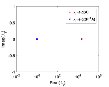
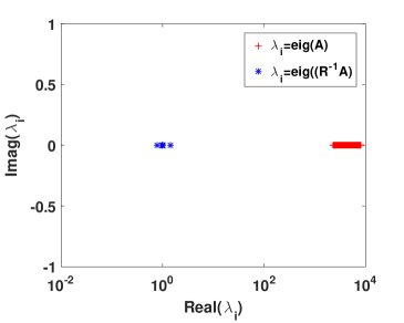
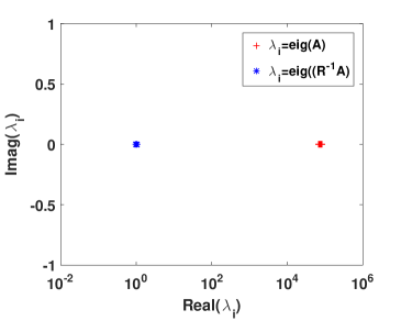
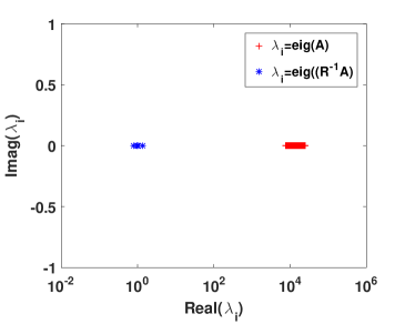
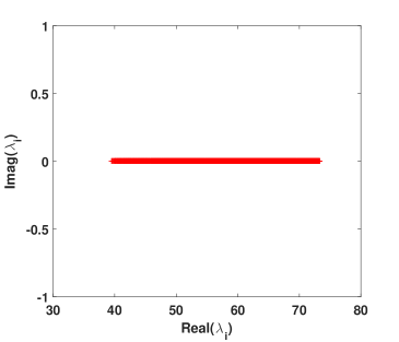
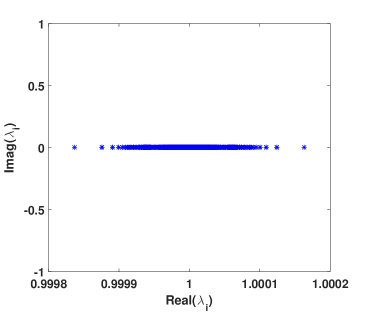
In Figs. 2-3, the eigenvalues of both the original matrix and the R. Chan’s preconditioned matrix for Example 7.1 with different are plotted. It can be seen that all the spectrum of the preconditioned matrix are well separated away from 0, and the eigenvalues lie within a small interval around 1, except for few outliers, which is in agreement with the theoretical analysis. It validates the robustness and effectiveness of the proposed preconditioner in terms of spectrum clustering.
In Tables 4-6, we compare the CPU time for solving Example 7.1 by the Cholesky method, the PCG method and the PCG-based GSF method with circulant preconditioners and . It shows that the CPU time of the PCG-based GSF method with and circulant preconditioners is much fewer than the Cholesky method. When , the Speed-up of the PCG-based GSF methods is more than five times, although the parameters , , and take different values. It also shows that the CPU time by the PCG-based GSF methods is less than that by the PCG methods. In addition, the iteration numbers of the PCG(R) method almost keep constant when is increasing rapidly, which verifies the superlinear convergence of the PCG method with R. Chan-based circulant preconditioner numerically. We also observe that the performances of the PCG-GSF(R) and PCG-GSF(S) methods are almost the same in terms of the CPU time. The proposed fast solution algorithm in Section 4 is better than the other testing methods.
| 8 | 1.369354e-05 | - | 2.371348e-05 | - | 3.576549e-05 | - |
|---|---|---|---|---|---|---|
| 16 | 3.405397e-06 | 2.0076 | 5.857784e-06 | 2.0173 | 8.708526e-06 | 2.0381 |
| 32 | 8.502827e-07 | 2.0018 | 1.460064e-06 | 2.0043 | 2.162141e-06 | 2.0100 |
| 64 | 2.124501e-07 | 2.0008 | 3.646990e-07 | 2.0013 | 5.395161e-07 | 2.0027 |
| 128 | 5.302274e-08 | 2.0024 | 9.107704e-08 | 2.0015 | 1.347362e-07 | 2.0015 |
| 4 | 7.332513e-05 | - | 5.407815e-05 | - | 3.758769e-05 | - |
|---|---|---|---|---|---|---|
| 8 | 1.931968e-05 | 1.9242 | 1.406583e-05 | 1.9429 | 9.608692e-06 | 1.9678 |
| 16 | 4.921064e-06 | 1.9730 | 3.570603e-06 | 1.9780 | 2.411094e-06 | 1.9947 |
| 32 | 1.241275e-06 | 1.9871 | 9.001434e-07 | 1.9879 | 6.055447e-07 | 1.9934 |
| 64 | 3.122634e-07 | 1.9910 | 2.272263e-07 | 1.9860 | 1.538685e-07 | 1.9765 |
| 1 | 1.063403e-06 | - | 8.405192e-07 | - | 6.396684e-07 | - |
|---|---|---|---|---|---|---|
| 2 | 2.730836e-07 | 1.9613 | 2.143924e-07 | 1.9710 | 1.618385e-07 | 1.9828 |
| 4 | 6.753548e-08 | 2.0156 | 5.205615e-08 | 2.0421 | 3.804022e-08 | 2.0890 |
| 8 | 1.565594e-08 | 2.1089 | 1.111329e-08 | 2.2278 | 6.956504e-09 | 2.4511 |
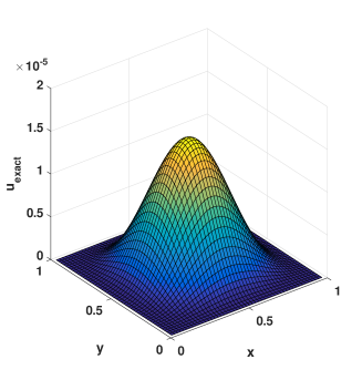
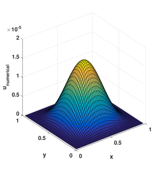
Example 7.2.
Consider the following 2D time distributed-order and Riesz space fractional diffusion-wave problem:
with , the exact solution is , and
where and ,

| GL-PCG() | GL-PCG() | ||||||||
|---|---|---|---|---|---|---|---|---|---|
| = | |||||||||
| 0.00 | 0.01 | 5.8 | 0.01 | 5.6 | 0.01 | 4.0 | |||
| 0.03 | 0.03 | 5.0 | 0.03 | 5.0 | 0.03 | 3.0 | |||
| 1.2 | 0.20 | 0.22 | 5.0 | 0.23 | 5.0 | 0.22 | 3.0 | ||
| 2.94 | 1.19 | 4.0 | 1.25 | 4.0 | 1.33 | 3.0 | |||
| 66.33 | 9.16 | 3.0 | 8.57 | 3.0 | 9.02 | 2.0 | |||
| 0.00 | 0.01 | 6.0 | 0.01 | 6.0 | 0.01 | 4.0 | |||
| 0.03 | 0.03 | 6.0 | 0.03 | 6.0 | 0.03 | 3.0 | |||
| 1.5 | 0.20 | 0.23 | 6.0 | 0.23 | 5.0 | 0.22 | 3.0 | ||
| 2.91 | 1.26 | 5.0 | 1.31 | 5.0 | 1.34 | 3.0 | |||
| 65.35 | 9.73 | 4.0 | 9.04 | 4.0 | 9.03 | 2.0 | |||
| 0.00 | 0.01 | 7.0 | 0.01 | 7.0 | 0.01 | 3.0 | |||
| 0.03 | 0.04 | 7.0 | 0.03 | 7.0 | 0.03 | 3.0 | |||
| 1.9 | 0.21 | 0.24 | 7.0 | 0.26 | 7.0 | 0.22 | 3.0 | ||
| 2.91 | 1.30 | 6.0 | 1.35 | 6.0 | 1.24 | 2.0 | |||
| 65.39 | 10.57 | 5.0 | 9.78 | 5.6 | 9.01 | 2.0 | |||
(a) Spectrum of (b) Spectrum of
(a) Spectrum of (b) Spectrum of
| GL-PCG() | GL-PCG() | ||||||||
|---|---|---|---|---|---|---|---|---|---|
| = | |||||||||
| 0.00 | 0.02 | 7.0 | 0.01 | 7.0 | 0.01 | 5.0 | |||
| 0.03 | 0.04 | 8.0 | 0.04 | 8.0 | 0.04 | 5.0 | |||
| 1.2 | 0.20 | 0.25 | 8.0 | 0.32 | 8.0 | 0.24 | 4.0 | ||
| 2.92 | 1.39 | 8.0 | 1.63 | 8.0 | 1.56 | 4.0 | |||
| 65.62 | 11.30 | 7.0 | 11.28 | 7.0 | 10.39 | 3.0 | |||
| 0.00 | 0.01 | 7.0 | 0.01 | 7.0 | 0.01 | 5.0 | |||
| 0.03 | 0.04 | 9.0 | 0.04 | 9.0 | 0.03 | 4.0 | |||
| 1.5 | 0.20 | 0.28 | 9.9 | 0.37 | 9.9 | 0.27 | 4.0 | ||
| 2.88 | 1.42 | 9.0 | 1.65 | 9.0 | 1.58 | 4.0 | |||
| 65.09 | 12.39 | 9.0 | 12.37 | 9.0 | 10.75 | 3.0 | |||
| 0.00 | 0.01 | 7.0 | 0.01 | 7.0 | 0.01 | 4.0 | |||
| 0.03 | 0.04 | 9.0 | 0.04 | 9.0 | 0.03 | 4.0 | |||
| 1.9 | 0.20 | 0.29 | 11.0 | 0.38 | 11.0 | 0.24 | 3.0 | ||
| 2.89 | 1.55 | 12.0 | 1.83 | 12.0 | 1.51 | 3.0 | |||
| 65.13 | 14.01 | 12.0 | 13.88 | 12.0 | 10.73 | 3.0 | |||
To verify the convergence order of the proposed difference scheme (6.11)-(6.13), in Tables 7-9, take , and . Let
where and represent the exact and numerical solutions at step sizes , and , respectively. The convergence orders are defined as
Tables 10-12 are to verify the efficiency of the proposed GL-PCG method with the truncated preconditioner described in Section 6.2. The resultant Sylvester matrix equations (6.16) of the 2D case are solved by using the Cholesky method, the PCG method, and the proposed GL-PCG method, respectively. The stopping criterions of the PCG and GL-PCG algorithms are
respectively, where is the -th residuals of the GL-PCG algorithm, and the initial guess in each time level is given as the zero matrix.
Besides the proposed truncated preconditioner , we also test the R. Chan’s-based BCCB preconditioner:
| GL-PCG() | GL-PCG() | ||||||||
|---|---|---|---|---|---|---|---|---|---|
| = | |||||||||
| 0.00 | 0.01 | 5.8 | 0.01 | 5.6 | 0.02 | 4.0 | |||
| 0.03 | 0.03 | 5.0 | 0.03 | 5.0 | 0.03 | 3.0 | |||
| 1.2 | 0.20 | 0.22 | 5.0 | 0.23 | 5.0 | 0.22 | 3.0 | ||
| 2.89 | 1.20 | 4.0 | 1.25 | 4.0 | 1.33 | 3.0 | |||
| 65.50 | 9.14 | 3.0 | 8.56 | 3.0 | 9.05 | 2.0 | |||
| 0.00 | 0.01 | 6.0 | 0.01 | 6.0 | 0.01 | 4.0 | |||
| 0.03 | 0.03 | 6.0 | 0.03 | 6.0 | 0.03 | 3.0 | |||
| 1.5 | 0.20 | 0.23 | 6.0 | 0.23 | 5.0 | 0.22 | 3.0 | ||
| 2.90 | 1.24 | 5.0 | 1.31 | 5.0 | 1.33 | 3.0 | |||
| 65.60 | 9.68 | 4.0 | 8.99 | 4.0 | 9.05 | 2.0 | |||
| 0.00 | 0.01 | 7.0 | 0.01 | 7.0 | 0.01 | 3.0 | |||
| 0.03 | 0.03 | 7.0 | 0.03 | 7.0 | 0.03 | 3.0 | |||
| 1.9 | 0.20 | 0.24 | 7.0 | 0.26 | 7.0 | 0.21 | 3.0 | ||
| 2.88 | 1.29 | 6.0 | 1.35 | 6.0 | 1.23 | 2.0 | |||
| 65.56 | 10.56 | 5.6 | 9.74 | 5.6 | 9.03 | 2.0 | |||
Figs. 4-5 present the comparisons of the exact and numerical solutions of the difference scheme (6.11)-(6.13) for Example 7.2 with different , and . We can see that the numerical solutions are in good agreement with the exact solutions.
The maximum errors and convergence orders of the numerical scheme (6.11)-(6.13) for Example 7.2 in space, time, and distributed order are displayed in Tables 7-9, respectively. One can be seen from these tables is that the convergence orders of the scheme (6.11)-(6.13) are two. The numerical convergence orders are in accordance with the expected ones.
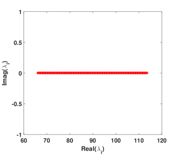
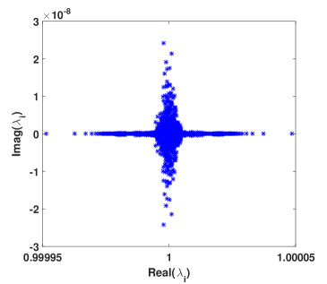
Figs. 6-7 show the distributions of the eigenvalues of both the original matrix and the proposed truncated preconditioned matrix () for Example 7.2. Clearly, the eigenvalues of are well grouped around 1 and separated away from 0, which confirms that the proposed truncated preconditioner exhibits very nice clustering properties.
Tables 10-12 report the numerical results for Example 7.2 by the Cholesky, PCG and GL-PCG methods with preconditioners and with . We can see that the GL-PCG method with preconditioner exhibits excellent performance. Specifically, the average number of iterations of the GL-PCG() method is much smaller than that of the PCG() and GL-PCG() methods, and it will not increase with the refinement of the spatial grids. It also shows that the performances of the PCG() and GL-PCG() methods are almost the same in terms of the CPU time and the average number of iterations. The performance of the proposed truncated preconditioner is better than the BCCB preconditioner.
8 Conclusion
In this paper, we propose efficient difference methods to solve the time distributed-order and Riesz space fractional diffusion-wave equations with initial-boundary value condition. The unconditional stability and second-order convergence in time, space, and distributed-order of the difference schemes are analyzed. The 1D discretizations lead to SPD Toeplitz linear systems, which are solved by the PCG-based GSF method with R. Chan’s circulant preconditioner. In the 2D case, the GL-PCG method with a truncated preconditioner is designed to solve the discretized SPD Sylvester matrix equations. Then we show that the convergences of the proposed iterative algorithms are very fast by proving the spectrums of the preconditioned matrices are clustered around one. Numerical experiments are carried out to demonstrate the effectiveness of the proposed numerical methods. In future work, We will work on developing other fast iterative algorithms and new efficient preconditioners to accelerate the convergence of numerical methods.
Acknowledgments
This work is supported by NSFC (61772003 and 11801463), the Applied Basic Research Project of Sichuan Province (20YYJC3482), and the Fundamental Research Funds for the Central Universities (JBK1902028).
References
- [1] J. Korbel, Y. Luchko, Modeling of financial processes with a space-time fractional diffusion equation of varying order, Fract. Calc. Appl. Anal. 19 (6) (2016) 1414–1433.
- [2] C. Ionescu, A. Lopes, D. Copot, J. A. T. Machado, J. H. T. Bates, The role of fractional calculus in modelling biological phenomena: a review, Commun. Nonlinear Sci. Numer. Simul. 51 (2017) 141–159.
- [3] D. Baleanu, R. L. Magin, S. Bhalekar, V. Daftardar-Gejji, Chaos in the fractional order nonlinear Bloch equation with delay, Commun. Nonlinear Sci. Numer. Simul. 25 (2015) 41–49.
- [4] A. H. Bhrawy, E. H. Doha, D. Baleanu, S. S. Ezz-Eldien, M. A. Abdelkawy, An accurate numerical technique for solving fractional optimal control problems, Proc. Rom. Acad. Ser. A Math. Phys. Tech. Sci. Inf. Sci. 16 (1) (2015) 47–54.
- [5] Y. Li, F. Liu, I. W. Turner, T. Li, Time-fractional diffusion equation for signal smoothing, Appl. Math. Comput. 326 (2018) 108–116.
- [6] R. Metzler, J. Klafter, The random walk’s guide to anomalous diffusion: a fractional dynamics approach, Phys. Rep. 339 (1) (2000) 1–77.
- [7] A. N. Kochubei, Distributed order calculus and equations of ultraslow diffusion, J. Math. Anal. Appl. 340 (1) (2007) 252–281.
- [8] A. V. Chechkin, R. Gorenflo, I. M. Sokolov, Retarding subdiffusion and accelerating superdiffusion governed by distributed-order fractional diffusion equations, Phys. Rev. E 66 (2002) 046129.
- [9] M. Caputo, Mean fractional-order-derivatives differential equations and filters, Annali Dell universit Di Ferrara 41 (1) (1995) 73–84.
- [10] R. Gorenflo, Y. Luchko, M. Stojanovi, Fundamental solution of a distributed order time-fractional diffusion-wave equation as probability density, Fract. Calc. Appl. Anal. 16 (2) (2013) 297–316.
- [11] Z. Li, Y. Luchko, M. Yamamoto, Analyticity of solutions to a distributed order time-fractional diffusion equation and its application to an inverse problem, Comput. Math. Appl. 73 (2016) 1041–1052.
- [12] H. Ye, F. Liu, V. Anh, Compact difference scheme for distributed-order time-fractional diffusion-wave equation on bounded domains, J. Comput. Phys. 298 (2015) 652–660.
- [13] S. Mashayekhi, M. Razzaghi, Numerical solution of distributed order fractional differential equations by hybrid functions, J. Comput. Phys. 315 (2016) 169–181.
- [14] W. Bu, A. Xiao, W. Zeng, Finite difference/finite element methods for distributed-order time fractional diffusion equations, J. Sci. Comput. 72 (3) (2017) 422–441.
- [15] M. Li, C. Huang, F. Jiang, Galerkin finite element method for higher dimensional multi-term fractional diffusion equation on non-uniform meshes, Appl. Anal. 96 (8) (2017) 1269–1284.
- [16] G.-H. Gao, Z.-Z. Sun, Two difference schemes for solving the one-dimensional time distributed-order fractional wave equations, Numer. Algor. 74 (2017) 675–697.
- [17] H. Jiang, F. Liu, I. Turner, K. Burrage, Analytical solutions for the multi-term time-space Caputo-Riesz fractional advection-diffusion equations on a finite domain, J. Math. Anal. Appl. 389 (2) (2012) 1117–1127.
- [18] G.-H. Gao, H.-W. Sun, Z.-Z. Sun, Some high-order difference schemes for the distributed-order differential equations, J. Comput. Phys. 298 (2015) 337–359.
- [19] H. Ye, F. Liu, V. Anh, I. Turner, Numerical analysis for the time distributed-order and Riesz space fractional diffusions on bounded domains, IMA J. Appl. Math. 80 (3) (2015) 825–838.
- [20] J. Pan, M. Ng, H. Wang, Fast preconditioned iterative methods for finite volume discretization of steady-state space-fractional diffusion equations, Numer. Algor. 74 (2017) 153–173.
- [21] M. Ng, Iterative Methods for Toeplitz Systems, Oxford Science Publications, 2004.
- [22] J. Pan, R. Ke, M. Ng, H.-W. Sun, Preconditioning techniques for diagonal-times-Toeplitz matrices in fractional diffusion equations, SIAM J. Sci. Comput. 36 (6) (2014) A2698–A2719.
- [23] R. Chan, G. Strang, Toeplitz equations by conjugate gradients with circulant preconditioner, SIAM J. Sci. Stat. Comput. 10 (1) (1989) 104–119.
- [24] X.-M. Gu, T.-Z. Huang, H.-B. Li, L. Li, W.-H. Luo, On -step CSCS-based polynomial preconditioners for Toeplitz linear systems with application to fractional diffusion equations, Appl. Math. Lett. 42 (2015) 53–58.
- [25] X.-M. Gu, T.-Z. Huang, B. Carpentieri, L. Li, C. Wen, A hybridized iterative algorithm of the BiCORSTAB and GPBiCOR methods for solving non-Hermitian linear systems, Comput. Math. Appl. 70 (12) (2015) 3019–3031.
- [26] H.-K. Pang, H.-W. Sun, Shift-invert Lanczos method for the symmetric positive semidefinite Toeplitz matrix exponential, Numer. Linear Algebra Appl. 18 (3) (2011) 603–614.
- [27] S.-L. Lei, H.-W. Sun, A circulant preconditioner for fractional diffusion equations, J. Comput. Phys. 242 (2013) 715–725.
- [28] S.-L. Lei, X. Chen, X. Zhang, Multilevel circulant preconditioner for high-dimensional fractional diffusion equations, East Asian J. Appl. Math. 6 (2) (2016) 109–130.
- [29] Y.-L. Zhao, P.-Y. Zhu, W.-H. Luo, A fast second-order implicit scheme for non-linear time-space fractional diffusion equation with time delay and drift term, Appl. Math. Comput. 336 (2018) 231–248.
- [30] M. Donatelli, M. Mazza, S. Serra-Capizzano, Spectral analysis and structure preserving preconditioners for fractional diffusion equations, J. Comput. Phys. 307 (2016) 262–279.
- [31] S. Karimi, Global conjugate gradient method for solving large general Sylvester matrix equation, J. Math. Model. 1 (1) (2013) 15–27.
- [32] S. S. Capizzano, E. Tyrtyshnikov, Any circulant-like preconditioner for multilevel matrices is not superlinear, SIAM J. Matrix Anal. Appl. 21 (2) (1999) 431–439.
- [33] S. S. Capizzano, Preconditioning strategies for asymptotically ill-conditioned block Toeplitz systems, BIT 34 (4) (1994) 579–594.
- [34] R. Chan, X.-Q. Jin, An Introduction to Iterative Toeplitz Solvers, SIAM, PA, 2007.
- [35] H.-Y. Jian, T.-Z. Huang, X.-L. Zhao, Y.-L. Zhao, A fast implicit difference scheme for a new class of time distributed-order and space fractional diffusion equations with variable coefficients, Adv. Difference Equ. 2018 (1) (2018) 205.
- [36] Z.-Z. Sun, G.-H. Gao, Finite Difference Methods for the Fractional Differential Equations, Science Press, Beijing, 2015, (in Chinese).
- [37] D. Wang, A. Xiao, W. Yang, Maximum-norm error analysis of a difference scheme for the space fractional CNLS, Appl. Math. Comput. 257 (2015) 241–251.
- [38] G.-X. Tian, T.-Z. Huang, Inequalities for the minimum eigenvalue of M-matrices, Electron. J. Linear Algebra 20 (1) (2013) 291–302.
- [39] Z.-Z. Sun, Z.-B. Zhang, A linearized compact difference scheme for a class of nonlinear delay partial differential equations, Appl. Math. Model. 37 (2013) 742–752.
- [40] M. Li, X.-M. Gu, C. Huang, M. Fei, G. Zhang, A fast linearized conservative finite element method for the strongly coupled nonlinear fractional Schrdinger equations, J. Comput. Phys. 358 (2018) 256–282.
- [41] X.-M. Gu, T.-Z. Huang, C.-C. Ji, B. Carpentieri, A. A. Alikhanov, Fast iterative method with a second order implicit difference scheme for time-space fractional convection-diffusion equations, J. Sci. Comput. 72 (2017) 957–985.
- [42] M. Ng, Circulant and skew-circulant splitting methods for Toeplitz systems, J. Comput. Appl. Math. 159 (1) (2003) 101–108.
- [43] M. Benzi, Preconditioning techniques for large linear systems: a survey, J. Comput. Phys. 182 (2) (2002) 418–477.
- [44] R. Chan, M. Ng, Conjugate gradient methods for Toeplitz systems, SIAM Rev. 38 (1996) 427–482.
- [45] W. R. Schneider, W. Wyss, Fractional diffusion and wave equations, J. Math. Physics 30 (1989) 134–144.
- [46] E. Orsingher, L. Beghin, Time-fractional telegraph equations and telegraph processes with Brownian time, Prob. Theory Rel. Fields 128 (2004) 141–160.
- [47] X.-M. Gu, T.-Z. Huang, X.-L. Zhao, H.-B. Li, L. Li, Strang-type preconditioners for solving fractional diffusion equations by boundary value methods, J. Comput. Appl. Math. 277 (2015) 73–86.