Time dependence of the flux of helium nuclei in cosmic rays measured by the PAMELA experiment between July 2006 and December 2009

Abstract

Precise time-dependent measurements of the Z = 2 component in the cosmic radiation provide crucial information about the propagation of charged particles through the heliosphere. The PAMELA experiment, with its long flight duration (15^th June 2006 - 23^rd January 2016) and the low energy threshold ($80$ MeV/n) is an ideal detector for cosmic ray solar modulation studies. In this paper, the helium nuclei spectra measured by the PAMELA instrument from July 2006 to December 2009 over a Carrington rotation time basis are presented. A state-of-the-art three-dimensional model for cosmic-ray propagation inside the heliosphere was used to interpret the time-dependent measured fluxes. Proton-to-helium flux ratio time profiles at various rigidities are also presented in order to study any features which could result from the different masses and local interstellar spectra shapes.

,

1 Introduction

Helium nuclei are the most abundant component of galactic cosmic rays (CRs) besides protons. They represent approximately $9\%$ of the total CR budget and together with protons account for $98\%$ of the cosmic radiation. The vast majority of helium nuclei are believed to be accelerated at astrophysical sources like supernovae remnants. Then, for several million of years before reaching the Earth’s Solar System, CRs had propagated through the Galaxy interacting with the interstellar matter and diffusing on the galactic magnetic field. These processes modify the CR spectral shapes and compositions with respect to the acceleration site. The precise measurement of the CR helium nuclei over an extended energy range is crucial in order to better understand both their origin and propagation history (e.g. Amato & Blasi (2018)). The most recent and most precise measurements of CR helium and proton spectra, provided by experiments such as PAMELA (Adriani et al., 2011), AMS-02 (Aguilar et al., 2015b, a), CREAM (Yoon et al., 2017) and ATIC (Panov et al., 2009), highlighted features in these spectra that challenged the commonly accepted scenario of CR acceleration and propagation in the Galaxy. However, the vast majority of CR measurements were obtained well inside the heliosphere where solar modulation affects the CR spectra.

When entering the heliosphere, CRs encounter the turbulent heliospheric magnetic field (HMF) embedded into the solar wind. Particles are scattered by HMF irregularities and undergo convection, diffusion, adiabatic deceleration and drift motions due to the presence of HMF gradients and curvatures. As a consequence, mostly below a few tens of GV, the CR intensities and spectral shapes change with respect to the Local Interstellar Spectra (LIS), i.e. the spectra which would be measured outside the heliospheric boundaries. This effect is known as solar modulation (e.g. Potgieter (2013, 2017)). The solar activity follows an $11$-year cycle which introduces a time dependence: higher CR intensity is measured during solar minimum, lower during solar maximum. Precise time-dependent measurements of low energy CRs improve the understanding of solar modulation. These studies are essential to calibrate models that describe mechanisms for the modulation of CRs in the heliosphere (e.g. Potgieter et al. (2014)). Furthermore, sophisticated models of particle transport in the heliosphere play a fundamental role in space weather and to predict radiation hazard for long-term spacecraft missions.

The PAMELA detector, due to its low energy limit and long flight duration, represents an ideal instrument to perform precise measurements of the time-dependent fluxes of different CR species. The PAMELA collaboration already published several papers on CR solar modulation: protons (Adriani et al., 2013; Martucci et al., 2018), electrons (Adriani et al., 2015) and positron-to-electron flux ratio (Adriani et al., 2016). In this paper the time-dependent helium spectra measured by the PAMELA instrument during the $23^{\rm rd}$ solar minimum (July 2006 - December 2009) are presented. The extraordinary quiet solar modulation period from 2006 to 2009 (e.g. Potgieter et al. (2015)) provides excellent opportunity to study CR propagation in the heliosphere under relative perfect modulation conditions (e.g. Di Felice et al. (2017)). The spectra were measured for each Carrington rotation period ($\approx 27$ days) assuring an optimal compromise between a good time resolution and a high statistic. The studied time period corresponds to Carrington rotation numbers $2045-2091$. No isotopic separation was performed in this work, consequently the fluxes correspond to the sum of ⁴He and ³He fluxes.

Additionally, helium nuclei fluxes are compared to that for protons, as a function of time and rigidity. From a solar modulation point of view, time-dependent proton-to-helium flux ratios may result from the different particle masses and from the different shapes of the local interstellar spectra (Tomassetti et al., 2018; Corti et al., 2019).

Finally, the modelling of these reported spectra, with a state-of-the-art 3D numerical model is presented. Excellent qualitative and good quantitative agreement between modelling results and the observed spectra is found.

2 The PAMELA detector

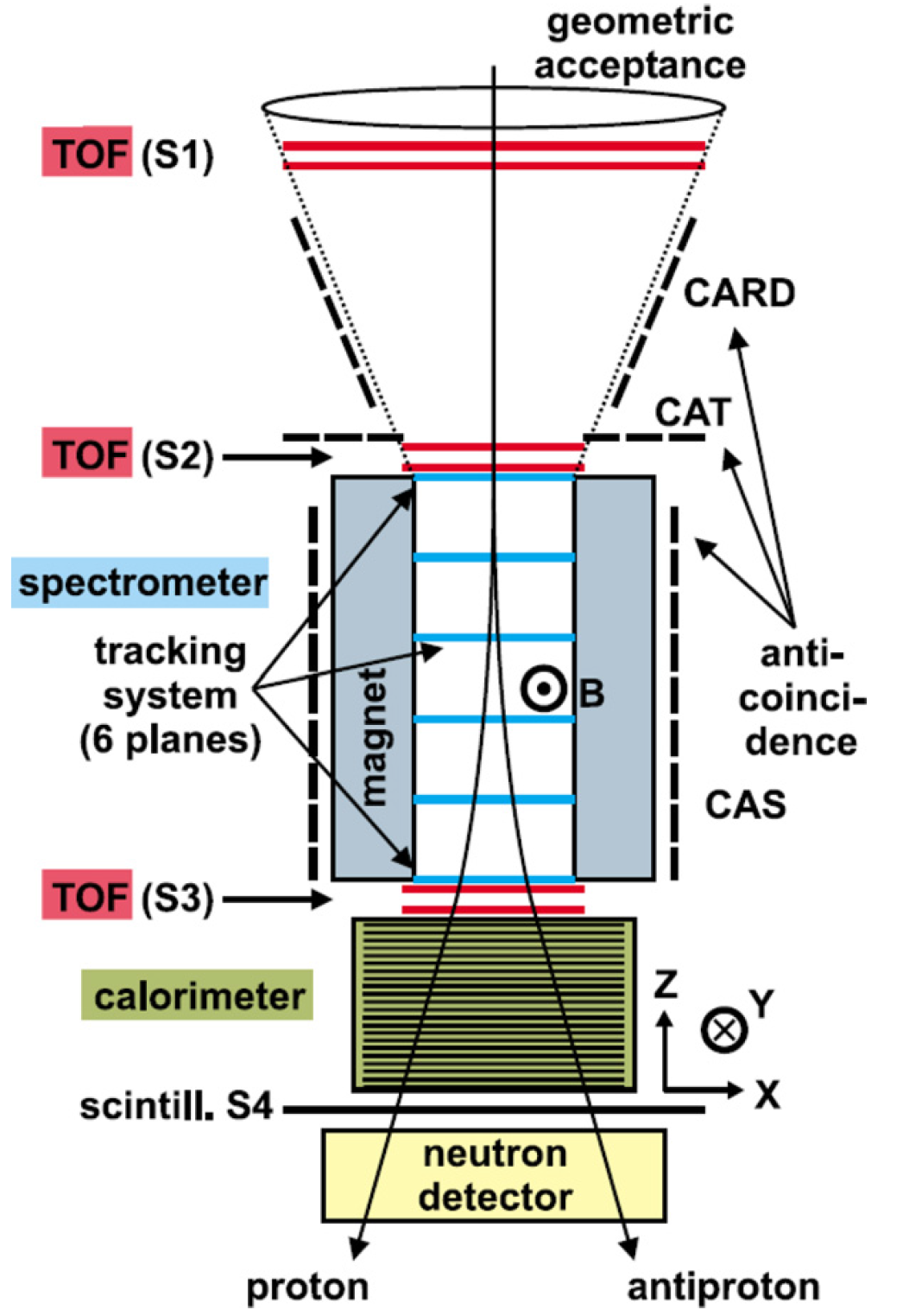
Figure 1: PAMELA and its sub-detectors.

PAMELA (Payload for Antimatter-Matter Exploration and Light-nuclei Astrophysics) is a satellite-borne experiment designed to make long duration observations of the cosmic radiation from Low Earth Orbit (Picozza et al., 2007). The PAMELA payload is schematically shown in Figure 1. The instrument collected galactic CRs for almost 10 years from 2006 June 15 when it was launched from the Baikonur cosmodrome in Kazakhstan, up to January 2016. The PAMELA instrument is hosted on board of the Russian satellite Resurs-DK1 with an elliptical orbit at an altitude ranging between 350 and 610 km with an inclination of $70^{\circ}$. After 2010 the orbit was changed to a circular one at a constant altitude of about $600$ km.

The payload comprises a number of redundant detectors capable of identifying particles by providing charge, rigidity and velocity measurements over a wide energy range. Multiple sub-detectors are built around a magnetic spectrometer, composed of a silicon tracking system (Adriani et al., 2003) placed inside a $0.43\$T permanent magnet. The $300$ $\mu$m thick double-sided Silicon sensors of the tracking system measure two impact coordinates on each plane, reconstructing with high accuracy the particle deflection with a maximum detectable rigidity of $\sim 1.2$ TV, and the absolute electric charge up to $Z\approx 8$.

A time of flight system (ToF) is composed of six layers of plastic scintillators, arranged in three double planes (S1, S2, and S3). The ToF, with a resolution of $\sim 300$ ps, provides a fast signal for data acquisition (Osteria et al., 2004). The trigger configuration is defined by coincidental energy deposit in S1, S2 and S3. The ToF also contributes to particle identification measuring through the ionization energy loss the absolute charge up to $Z\approx 6$ and the particle velocity and incoming direction that, together with the curvature measured by the tracking system, allows the charge sign to be determined.

An electromagnetic imaging W/Si calorimeter ($16.3$ radiation lengths and $0.6$ interaction lengths deep) provides hadron-lepton discrimination (Boezio et al., 2002). A neutron counter (Stozhkov et al., 2005) contributes to discrimination power by detecting the increased neutron production in the calorimeter associated with hadronic showers compared to electromagnetic ones, while a plastic scintillator, placed beneath the calorimeter, increases the identification of high-energy electrons. The whole apparatus is surrounded by an anti-coincidence system (AC) of three sets of scintillators (CARD, CAS, and CAT) for the rejection of background events (Orsi et al., 2005). A comprehensive description of the instrument can be found in Adriani et al. (2014).

3 Analysis

3.1 Event Selection

A clean sample of helium nuclei events was obtained applying cuts on the information provided by the PAMELA sub-detectors:

1. Only events with a single track fitted in the spectrometer and fully contained within $1.5$ mm away from the magnet walls and the ToF-scintillators edges were selected. The track of the selected events had to have a lever-arm of at least 4 silicon planes and a minimum of 3 hits on both the bending x-view and non-bending y-view. Low-quality tracks were rejected requiring a good $\chi^{2}$ resulting from the fit.

2. Down-going particles were selected requiring a positive $\beta=\frac{v}{c}$ ($v$ particle speed, $c$ speed of light) measured by the ToF system. This selection rejected splash albedo particles.

3. Helium nuclei were finally selected according to their mean energy release in terms of the minimum ionizing particle (MIP) over the silicon planes of the tracking system. Only events which were consistent with the helium band shown in Figure 2 were selected. Because of the energy losses, the minimum detectable rigidity for helium was on average $840$ MV, i.e. $\sim 90$ MeV/n in kinetic energy. Below this energy, helium nuclei were not able to reach S3 and trigger the data acquisition.

No attempt was made in this paper to separate between ³He and ⁴He nuclei, although separation is possible between 0.1 and 1.5 GeV/n (Adriani et al., 2016). Hence, in the analysis all Z=2 particles were treated as being ⁴He.

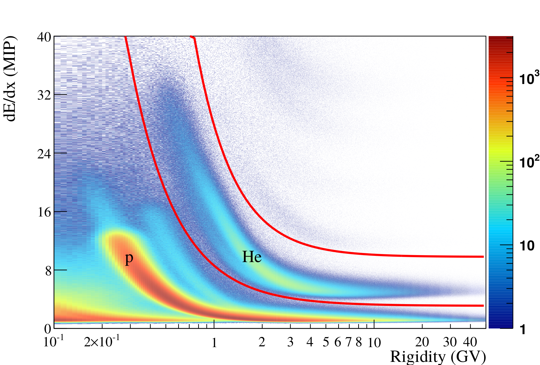
Figure 2: Distribution of the average ionization energy loss in terms of the minimum ionizing particle (MIP) inside the silicon tracker planes as a function of particle rigidity. The helium nuclei band is clearly separated from the hydrogen nuclei one.

3.2 Selection efficiencies

The redundant information provided by the PAMELA sub-detectors allowed to study the selection efficiencies with flight data. To account for any possible time variation of the detector response, the efficiencies were evaluated for each Carrington rotation. Simulated data were used to cross check the flight efficiencies. With the Monte Carlo data it was possible to reproduce and study all selection efficiencies, their rigidity and time dependence allowing to detect possible sources of bias, like contamination of efficiency samples and correlation among selection criteria.

The tracking system efficiency (criterion 1) and its energy dependence were obtained by Monte Carlo data. This efficiency was found to decrease over the years from a maximum of $\approx 90\%$ in $2006$ to $\approx 20\%$ at the end of $2009$. This significant time dependence was due to the sudden, random failure of a few front-end chips in the tracking system. This resulted in a progressive reduction of the number of hits available for track reconstruction which in turn produced a decreasing efficiency. The front-end chip failure was properly simulated with the inclusion in the Monte Carlo of a time-dependent map of dead channels. In order to decrease the statistical fluctuations, each efficiency was fitted with an appropriate function that reproduced its rigidity dependence. The values resulting from the fit were used to calculate the fluxes. Two samples of ⁴He and ³He were simulated in order to account for possible differences in the tracking efficiency for the two isotopes but no significant differences were found.

Similarly to the procedure adopted for the time-dependent analysis of the cosmic-ray protons (Adriani et al., 2013; Martucci et al., 2018), in order to account for any residual instrumental time-dependence, the fluxes of each Carrington rotation were normalized between $\approx 20$ and $50$ GV to the flux measured in the same rigidity region over the period July 2006 - March 2008 (Adriani et al., 2011).

Flight efficiency for criterion $3$ was obtained from a sample of helium nuclei selected by means of the ionization energy loss information provided by the ToF system. The selection efficiency was found to be constant with time and higher than $99\%$ in the whole rigidity range.

3.3 Statistical deconvolution

The helium rigidity measured with the tracking system differs from the initial rigidity at the top of the payload. This is due to the finite spectrometer resolution and the ionization energy losses suffered by the particles traversing the instrument. This latter effect was particularly relevant for helium nuclei below 2 GeV. A correction was applied by means of an unfolding procedure, following the Bayesian approach proposed by D’Agostini (1995). A detector response matrix was calculated with Monte Carlo data, one for each Carrington rotation under analysis. The unfolding procedure was applied to the count distributions of selected events binned according to their measured rigidities and divided by all selection efficiencies except those of the tracking system. The tracking system efficiency was instead applied to the unfolded count distribution.

3.4 Flux determination

The absolute helium flux $\Phi(E)$ in kinetic energy was obtained as follows:

$$\Phi(E)=\frac{N(E)}{G(E)\times T\times\epsilon(E)\times\Delta E}$$ (1)

where $N(E)$ is the unfolded count distribution, $\epsilon(E)$ the efficiency of the tracking system selections, $G(E)$ the geometrical factor, $T$ the live time and $\Delta E$ the width of the energy interval. For the conversion from rigidity to kinetic energy all helium nuclei events were treated as ⁴He.

Because of the wide geomagnetic region spanned by the satellite over its orbit, the helium nuclei spectrum was evaluated for various, seven, vertical geomagnetic cutoff intervals, estimated using the satellite position and the Störmer approximation. For each spectrum, only the fluxes estimated in energy regions at least 1.3 times above the maximum vertical geomagnetic cutoff of each interval were assumed to be of galactic origin. Finally, the helium nuclei spectrum was determined by combining such fluxes of each geomagnetic cutoff interval weighted for the corresponding fractional live time.

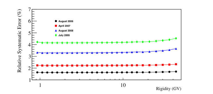
Figure 3: Relative systematic error as a function of rigidity for four time intervals.

3.4.1 Live time

The live time was provided by an on-board clock that timed the periods during which the apparatus was waiting for a trigger. The acquisition time was evaluated for each energy bin as the total live time spent above the geomagnetic cutoff and outside the South Atlantic Anomaly. The accuracy of the live time determination was cross-checked by comparing different clocks available in flight, which showed a relative difference of less than $0.2\%$. The total live time was about $5\times 10^{7}$ s above $∼20$ GV, reducing to about $18\%$ of this value at $800$ MV because of the relatively short time spent by the satellite at high geomagnetic latitudes.

3.4.2 Geometrical factor

The geometrical factor for this analysis was determined by the requirement of triggering and containment within the fiducial volume (criterion 1). The pure geometrical acceptance above $2$ GV is $19.5$ cm² sr. The geometrical factor, including interactions and energy losses, was estimated with the full simulation of the apparatus, and was found to be about $13\%$ lower because of fragmentation of helium nuclei in the instrument material above S3. Below 1 GV the acceptance sharply decreased because of the fluctuations in energy losses due to the particle slowdown.

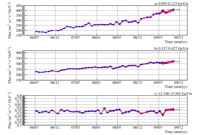
Figure 4: Time profiles of the helium flux for three kinetic energy intervals; the error bars are statistical, while the shaded area represents the quadratic sum of all systematic uncertainties.

4 Systematic uncertainties

Various sources of systematic uncertainties were analyzed:

1. The statistical errors resulting from the finite size of the efficiency samples. Most of the efficiencies were fitted in order to reduce the statistical fluctuations. For each efficiency a systematic uncertainty related to the fit estimation was obtained evaluating the one sigma ($68\%$) confidence intervals associated to the fitted values.

2. The live time uncertainty. As discussed in Section 3.4.1 the systematic uncertainty related to the live time was estimated to be constant at $0.2\%$ (Adriani et al., 2013).

3. The systematic error due to the unfolding procedure. This was evaluated by folding and unfolding a known spectral shape. A large sample of helium nuclei was simulated with an input spectrum consistent with the reconstructed experimental spectrum at the top of the payload. The rigidities of the simulated events were reconstructed and the count distribution was unfolded and compared with the initial simulated sample by means of pull distributions. More details on this procedure are reported by Adriani et al. (2015). A systematic uncertainty of $\approx 2\%$ was estimated.

4. The error associated to the flux normalization factor. This was assumed to be the statistical error on the ratio between the measured flux ($\approx 20-50$ GV) and the corresponding flux presented by Adriani et al. (2011).

The overall systematic uncertainty associated to the fluxes was obtained as the quadratic sum of all the contributions. Figure 3 shows the time dependence of the global systematic uncertainty as a function of the rigidity. The uncertainty increase over time was mainly due to the decreasing efficiency of the tracking system.

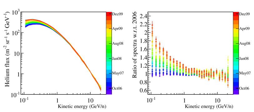
Figure 5: Left panel: the evolution of the helium energy spectrum as particle intensities approached the period of minimum solar activity, from July 2006 (violet), to December 2009 (red). Right panel: the ratio of the measured spectra with respect to the spectrum of July 2006. Different time periods are color-coded on the right of each panel. The error bars are the result of the quadratic sum of statistical and systematic errors.

5 Results

Figure 4 shows the time profile of the helium flux for three kinetic energy intervals. The last four Carrington rotations of 2009 were combined in a single spectrum for statistical reasons. A total of 42 spectra were measured. The error bars are statistical, while the shaded areas represent the quadratic sum of all systematic uncertainties. These plots show the different amount of solar modulation as a function of the energy. The flux measured at about 100 MeV/n increased by a factor 2 from middle $2006$ to the end of $2009$ while the flux at $600$ MeV/n increased only by a factor $1.25$. Above $\approx 15$ GeV/n the effect of modulation was lower than the statistical precision of the measurement.

Figure 5, left panel, shows the time evolution of helium energy spectra from July 2006 (violet curve) to December 2009 (red curve). Figure 5, right panel, shows the ratio of the helium fluxes with respect to the fluxes measured in July $2006$. Besides the time-dependent intensity, a varying spectral shape was also observed over time. In $2006$ the maximum flux intensity was reached at about $250$ MeV/n slowly decreasing to about $150$ MeV/n by the end of $2009$. Table 1 presents the helium nuclei spectra measured over four time periods (Carrington rotations 2050, 2064, 2077 and 2088-2091).

Finally the solar modulation of the helium nuclei was compared to the published PAMELA proton spectrum evaluated during the same time period (Adriani et al., 2013). Also for the protons the last four Carrington rotations of 2009 were combined to form an average spectrum.

Figure 6 shows the proton-to-helium flux ratio as a function of time for five different rigidity intervals. The proton and helium fluxes were estimated as a function of rigidity, i.e. particles per m² sr s GV. Since the quantity measured by the magnetic spectrometer is rigidity, this approach allows a more precise estimation of the ratios considering that all systematic uncertainties, related to the same instrumental effects, cancel out. The residual systematic uncertainty includes only the errors due to the efficiency estimation. The error bars in Figure 6 represent the quadratic sum of the statistical errors with this residual systematic error.

A non constant ratio points to modulation differences between protons and helium which is further discussed below. The colored lines on Figure 6 represent a fit with a first degree polynomial function of the form $p_{0}+t\cdot p_{1}$ where $p_{0}$ is a normalization value, $p_{1}$ quantifies the amount of time dependence and $t$ is time. Above $1$ GV the proton-to-helium flux ratio over time was well described by a constant value. On the contrary, below $1$ GV the fit indicates an overall decrease of about $10\%$ from 2006 to 2009. However, because of the relatively large errors below $1$ GV, a time independence of the proton-to-helium flux ratio cannot be excluded also at these low rigidities.

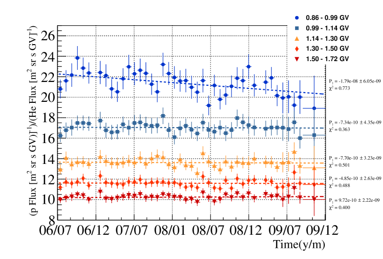
Figure 6: Time profiles of proton-to-helium flux ratio in five different rigidity intervals reported in the legend. The error bars are the result of the quadratic sum of statistical and systematic errors. For more details see the text.

In addition to the long-term decrease, below 1 GV the proton-to-helium flux ratio shows a cyclic variation with maxima registered during October 2006, August 2007, December 2007, August 2008 and March 2009. These short-term variations are beyond the scope of this paper and will be addressed in a future work.

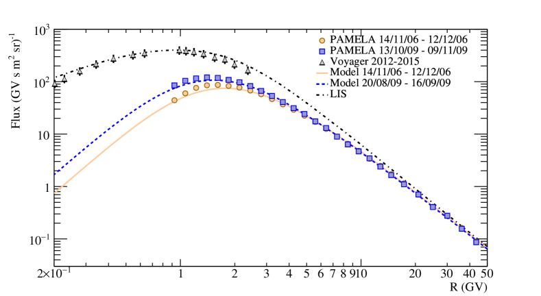
Figure 7: Computed helium fluxes as a function of rigidity for November 2006 and October 2009 (solid and dashed lines) compared with the measured fluxes by PAMELA (circles and squares). The dot-dashed line represents the LIS specified at 120 astronomical units used as input for the model. The triangular points are the fluxes measured by Voyager 1 outside the heliosphere (Cummings et al., 2016).

6 Data Interpretation and Discussion

A full three-dimensional cosmic-ray propagation model for describing CR modulation throughout the heliosphere, already applied to reproduce the PAMELA proton, electron and positron spectra, was used to determine the differential intensity of cosmic-ray helium nuclei at Earth from $20$ MV to $50$ GV. This steady-state model is based on the numerical solution of the Parker transport equation and has been extensively described, and applied to interpreting observations, by Potgieter et al. (2014, 2015); Di Felice et al. (2017) and recently by Aslam et al. (2019); Corti et al. (2019).

Following the approach of Bisschoff et al. (2019) , the LIS computation was performed s eparately for ³He and ⁴He. First, ³He and ⁴He LIS were obtained with the GALPROP code (Strong & Moskalenko, 1998) and then modified in order to reproduce the low energy Voyager 1 helium nuclei fluxes measured when the spacecraft entered the local interstellar medium in August 2012 (Cummings et al., 2016). The diffusion coefficients used for the computation, as well as all the other relevant heliospheric parameters, were essentially the same as obtained for the proton modeling described in Potgieter & Vos (2016). The modulated ³He and ⁴He spectra, were converted from kinetic energy per nucleon to rigidity and added together to obtain the total helium nuclei spectra presented in Figure 7.

The solid and the dash lines shown in Figure 7 represent the computed spectra for helium nuclei respectively for the Carrington rotation number 2050 (14 November - 12 December 2006) and 2089 (13 October - 9 November 2009). The model is in agreement with the measurements within the statistical and systematic errors for 2006 and 2009 above 2.5 GV. Below this energy the model is systematically lower by $10-15\%$ with respect to observational data. It is emphasized that the heliospheric parameters for helium modulation cannot be changed arbitrarily from those for protons to improve the quantitative agreements between the modelling results and these observations. There is no compelling reason to believe that GCR helium is modulated in a fundamentally different way with respect from GCR protons. However, some adjustments may be made to the LIS for helium, but because it is constrained by the mentioned Voyager 1 observations at low rigidity and by PAMELA observations at high rigidity where modulation is negligible, only minor adjustments have been made to the one published by Bisschoff et al. (2019) to obtain a LIS as shown in Figure 7. Therefore the LIS is assumed to be optimal in reproducing the observed spectra for the two periods at Earth over this wide rigidity range. Qualitatively, the modelling reproduces how the spectra became gradually softer as more low energy particles arrive at the Earth with decreasing solar activity to reach the maximum value in December 2009.

When the ratio of the computed proton and helium fluxes is calculated as a function of time, it gives an overall decrease from 2006 to 2009 of about $20\%$ at $200$ MV while no significant variation is predicted above $\sim 2$ GV. This results are in agreement with the observed ratios.

If there is no fundamental difference between proton and helium modulation in the heliosphere, a non-constant proton-to-helium flux ratio over time, for a given rigidity, is the result of:

1. their different velocities, related to the different particle masses (which play a role in the effective rigidity dependence of the various diffusion coefficients as well as the drift coefficient);

2. the different shape of the proton LIS compared to the helium LIS.

Using the proton and helium LIS from Bisschoff et al. (2019) it can be noticed that the different shapes of the two LIS result in a proton-to-helium flux ratio that, below 30 GV, increases progressively with decreasing rigidity, even significantly below 2 GV. When this ratio additionally changes with time, it means that the difference in the slopes of these LISs causes the effects of adiabatic energy losses to be somewhat different for helium than for protons when the overall modulation conditions change, as happened from 2006 to 2009. Moreover, the flux of CRs with lower rigidity reaches a maximum value at Earth later than the flux with higher rigidity when minimum solar activity had occurred. Following maximum solar activity, low rigidity CRs will reach a minimum value first, see e.g le Roux & Potgieter (1992); Potgieter & le Roux (1992).

A detailed description of the modelling along with a more quantitative study of the relative contribution of 1) and 2) to the observed time-dependent proton-to-helium flux ratio will be presented in a future publication. The analysis of the PAMELA data is still in progress to extend the time-dependent spectra of the helium nuclei to the $24^{th}$ solar maximum up to the reversal of heliospheric magnetic field polarity. This will cover the gap and overlap with the results recently published by the AMS-02 collaboration that reported a time-dependent proton-to-helium flux ratio between $\approx 2$ and 3 GV in the period between 2011 and 2017 (Aguilar et al., 2018).

The results discussed in this paper will be available at the Cosmic Ray Data Base of the ASI Space Science Data Center (http://tools.asdc.asi.it/CosmicRays/chargedCosmicRays.jsp).

Table 1: Helium nuclei fluxes measured by PAMELA over four time periods (Carrington rotations 2050, 2064, 2077 and 2088-2091). The first and second errors represent the statistical and systematic errors, respectively.

Kinetic Energy	Flux
(GeV/n)	(particles/(m2 sr s GeV))
	2006/11/14-2006/12/12	2007/12/01-2007/12/29	2008/11/20-2008/12/17	2009/09/16-2010/01/03
0.095-0.124	(1.99 $\pm$ 0.05 $\pm$ 0.05)$\times 10^{2}$	(2.56 $\pm$ 0.05 $\pm$ 0.06)$\times 10^{2}$	(2.94 $\pm$ 0.08 $\pm$ 0.08)$\times 10^{2}$	(4.08 $\pm$ 0.14 $\pm$ 0.22)$\times 10^{2}$
0.124-0.160	(2.41 $\pm$ 0.05 $\pm$ 0.05)$\times 10^{2}$	(3.09 $\pm$ 0.05 $\pm$ 0.08)$\times 10^{2}$	(3.35 $\pm$ 0.08 $\pm$ 0.10)$\times 10^{2}$	(4.31 $\pm$ 0.13 $\pm$ 0.23)$\times 10^{2}$
0.160-0.206	(2.78 $\pm$ 0.04 $\pm$ 0.07)$\times 10^{2}$	(3.38 $\pm$ 0.05 $\pm$ 0.08)$\times 10^{2}$	(3.67 $\pm$ 0.07 $\pm$ 0.11)$\times 10^{2}$	(4.44 $\pm$ 0.11 $\pm$ 0.23)$\times 10^{2}$
0.206-0.264	(2.84 $\pm$ 0.04 $\pm$ 0.07)$\times 10^{2}$	(3.32 $\pm$ 0.04 $\pm$ 0.08)$\times 10^{2}$	(3.60 $\pm$ 0.06 $\pm$ 0.10)$\times 10^{2}$	(4.15 $\pm$ 0.10 $\pm$ 0.22)$\times 10^{2}$
0.264-0.337	(2.66 $\pm$ 0.03 $\pm$ 0.06)$\times 10^{2}$	(3.04 $\pm$ 0.04 $\pm$ 0.07)$\times 10^{2}$	(3.29 $\pm$ 0.05 $\pm$ 0.09)$\times 10^{2}$	(3.81 $\pm$ 0.08 $\pm$ 0.20)$\times 10^{2}$
0.337-0.427	(2.37 $\pm$ 0.02 $\pm$ 0.06)$\times 10^{2}$	(2.71 $\pm$ 0.02 $\pm$ 0.06)$\times 10^{2}$	(2.84 $\pm$ 0.04 $\pm$ 0.08)$\times 10^{2}$	(3.22 $\pm$ 0.05 $\pm$ 0.17)$\times 10^{2}$
0.427-0.537	(2.06 $\pm$ 0.03 $\pm$ 0.05)$\times 10^{2}$	(2.34 $\pm$ 0.02 $\pm$ 0.05)$\times 10^{2}$	(2.42 $\pm$ 0.03 $\pm$ 0.07)$\times 10^{2}$	(2.69 $\pm$ 0.05 $\pm$ 0.14)$\times 10^{2}$
0.537-0.670	(1.71 $\pm$ 0.02 $\pm$ 0.04)$\times 10^{2}$	(1.89 $\pm$ 0.02 $\pm$ 0.04)$\times 10^{2}$	(1.97 $\pm$ 0.02 $\pm$ 0.06)$\times 10^{2}$	(2.17 $\pm$ 0.04 $\pm$ 0.12)$\times 10^{2}$
0.670-0.831	(1.39 $\pm$ 0.01 $\pm$ 0.03)$\times 10^{2}$	(1.50 $\pm$ 0.01 $\pm$ 0.04)$\times 10^{2}$	(1.56 $\pm$ 0.02 $\pm$ 0.04)$\times 10^{2}$	(1.74 $\pm$ 0.03 $\pm$ 0.09)$\times 10^{2}$
0.831-1.023	(1.08 $\pm$ 0.01 $\pm$ 0.02)$\times 10^{2}$	(1.16 $\pm$ 0.01 $\pm$ 0.03)$\times 10^{2}$	(1.20 $\pm$ 0.01 $\pm$ 0.03)$\times 10^{2}$	(1.30 $\pm$ 0.02 $\pm$ 0.07)$\times 10^{2}$
1.02-1.25	(8.27 $\pm$ 0.07 $\pm$ 0.20)$\times 10^{1}$	(8.81 $\pm$ 0.07 $\pm$ 0.21)$\times 10^{1}$	(9.12 $\pm$ 0.11 $\pm$ 0.26)$\times 10^{1}$	(9.71 $\pm$ 0.17 $\pm$ 0.51)$\times 10^{1}$
1.25-1.52	(6.38 $\pm$ 0.06 $\pm$ 0.15)$\times 10^{1}$	(6.73 $\pm$ 0.06 $\pm$ 0.16)$\times 10^{1}$	(6.89 $\pm$ 0.09 $\pm$ 0.20)$\times 10^{1}$	(7.17 $\pm$ 0.13 $\pm$ 0.38)$\times 10^{1}$
1.52-1.83	(4.83 $\pm$ 0.05 $\pm$ 0.11)$\times 10^{1}$	(5.02 $\pm$ 0.05 $\pm$ 0.12)$\times 10^{1}$	(5.05 $\pm$ 0.07 $\pm$ 0.15)$\times 10^{1}$	(5.34 $\pm$ 0.11 $\pm$ 0.29)$\times 10^{1}$
1.83-2.20	(3.60 $\pm$ 0.04 $\pm$ 0.09)$\times 10^{1}$	(3.71 $\pm$ 0.04 $\pm$ 0.09)$\times 10^{1}$	(3.72 $\pm$ 0.06 $\pm$ 0.11)$\times 10^{1}$	(3.91 $\pm$ 0.08 $\pm$ 0.20)$\times 10^{1}$
2.20-2.62	(2.62 $\pm$ 0.03 $\pm$ 0.06)$\times 10^{1}$	(2.72 $\pm$ 0.03 $\pm$ 0.06)$\times 10^{1}$	(2.88 $\pm$ 0.05 $\pm$ 0.08)$\times 10^{1}$	(2.83 $\pm$ 0.07 $\pm$ 0.15)$\times 10^{1}$
2.62-3.11	(1.84 $\pm$ 0.02 $\pm$ 0.04)$\times 10^{1}$	(1.90 $\pm$ 0.02 $\pm$ 0.04)$\times 10^{1}$	(2.04 $\pm$ 0.04 $\pm$ 0.06)$\times 10^{1}$	(1.97 $\pm$ 0.05 $\pm$ 0.10)$\times 10^{1}$
3.11-3.68	(1.34 $\pm$ 0.02 $\pm$ 0.03)$\times 10^{1}$	(1.39 $\pm$ 0.02 $\pm$ 0.03)$\times 10^{1}$	(1.47 $\pm$ 0.03 $\pm$ 0.04)$\times 10^{1}$	(1.45 $\pm$ 0.04 $\pm$ 0.07)$\times 10^{1}$
3.68-4.34	9.80 $\pm$ 0.15 $\pm$ 0.23	9.77 $\pm$ 0.15 $\pm$ 0.23	9.91 $\pm$ 0.21 $\pm$ 0.28	(1.04 $\pm$ 0.03 $\pm$ 0.05)$\times 10^{1}$
4.34-5.10	6.85 $\pm$ 0.09 $\pm$ 0.16	7.00 $\pm$ 0.10 $\pm$ 0.17	6.88 $\pm$ 0.14 $\pm$ 0.22	7.10 $\pm$ 0.21 $\pm$ 0.39
5.10-5.97	5.02 $\pm$ 0.07 $\pm$ 0.12	5.13 $\pm$ 0.07 $\pm$ 0.12	5.27 $\pm$ 0.11 $\pm$ 0.15	4.94 $\pm$ 0.16 $\pm$ 0.27
5.97-6.98	3.47 $\pm$ 0.06 $\pm$ 0.08	3.40 $\pm$ 0.06 $\pm$ 0.08	3.70 $\pm$ 0.08 $\pm$ 0.10	3.79 $\pm$ 0.12 $\pm$ 0.19
6.98-8.57	2.32 $\pm$ 0.04 $\pm$ 0.06	2.33 $\pm$ 0.04 $\pm$ 0.05	2.26 $\pm$ 0.06 $\pm$ 0.07	2.35 $\pm$ 0.08 $\pm$ 0.12
8.57-10.46	1.41 $\pm$ 0.03 $\pm$ 0.03	1.41 $\pm$ 0.03 $\pm$ 0.03	1.41 $\pm$ 0.04 $\pm$ 0.04	1.41 $\pm$ 0.06 $\pm$ 0.08
10.46-12.75	(8.25 $\pm$ 0.15 $\pm$ 0.20)$\times 10^{-1}$	(8.28 $\pm$ 0.16 $\pm$ 0.21)$\times 10^{-1}$	(8.22 $\pm$ 0.23 $\pm$ 0.25)$\times 10^{-1}$	(8.10 $\pm$ 0.34 $\pm$ 0.46)$\times 10^{-1}$
12.75-15.50	(5.53 $\pm$ 0.11 $\pm$ 0.13)$\times 10^{-1}$	(5.32 $\pm$ 0.11 $\pm$ 0.13)$\times 10^{-1}$	(5.49 $\pm$ 0.17 $\pm$ 0.17)$\times 10^{-1}$	(5.66 $\pm$ 0.25 $\pm$ 0.32)$\times 10^{-1}$
15.50-18.82	(3.25 $\pm$ 0.08 $\pm$ 0.08)$\times 10^{-1}$	(3.17 $\pm$ 0.08 $\pm$ 0.08)$\times 10^{-1}$	(2.96 $\pm$ 0.12 $\pm$ 0.10)$\times 10^{-1}$	(3.22 $\pm$ 0.17 $\pm$ 0.18)$\times 10^{-1}$
18.82-22.80	(1.80 $\pm$ 0.05 $\pm$ 0.04)$\times 10^{-1}$	(1.83 $\pm$ 0.06 $\pm$ 0.05)$\times 10^{-1}$	(2.09 $\pm$ 0.09 $\pm$ 0.07)$\times 10^{-1}$	(1.64 $\pm$ 0.12 $\pm$ 0.10)$\times 10^{-1}$

References

- Adriani et al. (2003) Adriani, O., Bonechi, L., Bongi, M., et al. 2003, Nuclear Instruments and Methods in Physics Research A, 511, 72
- Adriani et al. (2011) Adriani, O., Barbarino, G. C., Bazilevskaya, G. A., et al. 2011, Science, 332, 69
- Adriani et al. (2011) Adriani, O., Barbarino, G. C., Bazilevskaya, G. A., et al. 2011, Science, 332, 69
- Adriani et al. (2013) —. 2013, ApJ, 765, 91
- Adriani et al. (2014) —. 2014, Phys. Rep., 544, 323
- Adriani et al. (2015) —. 2015, ApJ, 810, 142
- Adriani et al. (2016) Adriani, O., Barbarino, G. C., Bazilevskaya, G. A., et al. 2016, The Astrophysical Journal, 818, 68
- Adriani et al. (2016) Adriani, O., Barbarino, G. C., Bazilevskaya, G. A., et al. 2016, Physical Review Letters, 116, 241105
- Aguilar et al. (2015a) Aguilar, M., Aisa, D., Alpat, B., et al. 2015a, Phys. Rev. Lett., 115, 211101
- Aguilar et al. (2015b) —. 2015b, Phys. Rev. Lett., 114, 171103
- Aguilar et al. (2018) Aguilar, M., Ali Cavasonza, L., Alpat, B., et al. 2018, Phys. Rev. Lett., 121, 051101
- Amato & Blasi (2018) Amato, E., & Blasi, P. 2018, Adv. Space Res., 62, 2731
- Aslam et al. (2019) Aslam, O. P. M., Bisschoff, D., Potgieter, M. S., Boezio, M., & Munini, R. 2019, ApJ, 873, 70
- Bisschoff et al. (2019) Bisschoff, D., Potgieter, M. S., & Aslam, O. P. M. 2019, ApJ, 878, 59:1
- Boezio et al. (2002) Boezio, M., Bonvicini, V., Mocchiutti, E., et al. 2002, Nuclear Instruments and Methods in Physics Research A, 487, 407
- Corti et al. (2019) Corti, C., Potgieter, M. S., Bindi, V., et al. 2019, ApJ, 871, 253
- Cummings et al. (2016) Cummings, A. C., Stone, E. C., Heikkila, B. C., et al. 2016, ApJ, 831, 18
- D’Agostini (1995) D’Agostini, G. 1995, Nuclear Instruments and Methods in Physics Research A, 362, 487
- Di Felice et al. (2017) Di Felice, V., Munini, R., Vos, E., & Potgieter, M. 2017, ApJ, 834, 89:1
- le Roux & Potgieter (1992) le Roux, J. A., & Potgieter, M. S. 1992, ApJ, 390, 661
- Martucci et al. (2018) Martucci, M., Munini, R., Boezio, M., et al. 2018, ApJ, 854, L2
- Orsi et al. (2005) Orsi, S., Carlson, P., Hofverberg, P., Lund, J., & Pearce, M. 2005, International Cosmic Ray Conference, 3, 369
- Osteria et al. (2004) Osteria, G., Campana, D., Barbarino, G., et al. 2004, Nuclear Instruments and Methods in Physics Research A, 535, 152
- Panov et al. (2009) Panov, A. D., Jr., J. H. A., Ahn, H. S., Bashinzhagyan, G. L., & Watts, J. W. 2009, Bull. Rus. Acad. Sci. Phys., 73, 564
- Picozza et al. (2007) Picozza, P., Galper, A. M., Castellini, G., et al. 2007, Astroparticle Physics, 27, 296
- Potgieter (2013) Potgieter, M. S. 2013, Space Sci. Rev., 176, 165
- Potgieter (2017) Potgieter, M. S. 2017, Adv. Space Res., 60, 848–864
- Potgieter & le Roux (1992) Potgieter, M. S., & le Roux, J. A. 1992, ApJ, 392, 300
- Potgieter & Vos (2016) Potgieter, M. S., & Vos, E. E. 2016, Journal of Physics: Conference Series, 767, 012018
- Potgieter et al. (2014) Potgieter, M. S., Vos, E. E., Boezio, M., et al. 2014, Solar Phys., 289, 391
- Potgieter et al. (2015) Potgieter, M. S., Vos, E. E., Munini, R., Boezio, M., & Di Felice, V. 2015, ApJ, 810, 141
- Stozhkov et al. (2005) Stozhkov, Y. I., Basili, A., Bencardino, R., et al. 2005, International Journal of Modern Physics A, 20, 6745
- Strong & Moskalenko (1998) Strong, A. W., & Moskalenko, I. V. 1998, ApJ, 509, 212
- Tomassetti et al. (2018) Tomassetti, N., Barão, F., Bertucci, B., et al. 2018, Phys. Rev. Lett., 121, 251104
- Yoon et al. (2017) Yoon, Y. S., Anderson, T., Barrau, A., et al. 2017, ApJ, 839, 5