Sigma Delta quantization for images
Abstract
In signal quantization, it is well-known that introducing adaptivity to quantization schemes can improve their stability and accuracy in quantizing bandlimited signals. However, adaptive quantization has only been designed for one-dimensional signals. The contribution of this paper is two-fold: i). we propose the first family of two-dimensional adaptive quantization schemes that maintain the same mathematical and practical merits as their one-dimensional counterparts, and ii). we show that both the traditional 1-dimensional and the new 2-dimensional quantization schemes can effectively quantize signals with jump discontinuities. These results immediately enable the usage of adaptive quantization on images. Under mild conditions, we show that the adaptivity is able to reduce the reconstruction error of images from the presently best to the much smaller , where is the number of jump discontinuities in the image and () is the total number of samples. This -fold error reduction is achieved via applying a total variation norm regularized decoder, whose formulation is inspired by the mathematical super-resolution theory in the field of compressed sensing. Compared to the super-resolution setting, our error reduction is achieved without requiring adjacent spikes/discontinuities to be well-separated, which ensures its broad scope of application.
We numerically demonstrate the efficacy of the new scheme on medical and natural images. We observe that for images with small pixel intensity values, the new method can significantly increase image quality over the state-of-the-art method.
1 Introduction
1.1 Quantization
In signal processing, quantization is the operation in which a signal’s real-valued samples get converted into a finite number of bits. As such, quantization digitizes the signal and makes it ready for digital processing. Mathematically, given a signal class and a fixed codebook , the goal of quantization is to map every signal in to a codebook representation that can be stored digitally. We use to denote the quantization map between the signal space and the codebook
In order to digitally restore the original signals, we usually assign a decoder, also called a reconstruction algorithm, to each quantization scheme. The decoder then recovers each signal from their encoded bits up to a small error. To ensure practicability, we only consider decoders that run in polynomial time. Let be a decoder, the error in the decoded signal is called distortion
For a given signal class , we define the optimal quantization to be the one that minimizes the distortion subject to a fixed bit budget. More precisely, let the fixed bit budget be , then among all codebooks that are representable in bits and all quantization maps from to , the optimal quantization is the one that minimizes the minimax distortion
where is the set of polynomial-time decoders.
When the signal class forms a compact set in a metric space, an optimal quantization can be found through the following information-theoretic argument. Given a fixed error tolerance level , one can find for the signal class an -net with the minimum possible cardinality , known as the covering number of . With this optimal -net, we carry out the quantization as follows. First, we assign the center of each -ball a symbol in the codebook (different centers are assigned different symbols). Then for each point/signal in , we quantize it to the symbol of the closest center. The total number of symbols used in this quantization equals the number of centers, , so they can be encoded in bits. This encoding is optimal as by definition, is the minimal cardinality of the net needed to cover the set. For the special case of being the unit -ball in , we have and or equivalently, (see, e.g., [7, 8, 37]). This is known as the exponential rate-distortion relation: the error decays exponentially with the number of bits. However, the quantization built this way suffers from the following impracticalities: 1) unless has a regular shape, the computation of the optimal -net of is subject to the curse of dimensionality; and 2) since the nearest center to a signal can only be found after all samples of that signal are received, this scheme cannot be operated in an online manner.
These issues inspire people to impose the following requirements on the quantization:
-
•
the quantization of a vector should have the same length as ;
-
•
the quantization should be operated in an online manner, which means (the entry of ) only depends on the past and current inputs , not the future ones ;
-
•
the alphabets for each are the same and fixed in advance, i.e., . Together they form the codebook ;
-
•
since quantization is implemented in the analog hardware, the mathematical operations involved should be as simple as possible. In particular, addition and subtraction are preferred over multiplication and division.
Here, for simplicity, we set the alphabet to be a bounded, evenly spaced grid with step-size ,
| (1.1) |
where , , and are pre-selected numbers.
1.2 Memoryless scalar quantization and Sigma Delta quantization
To avoid distraction, we review the existing quantization schemes directly in the context of image quantization. Let be the matrix that stores the pixel values of a grayscale image. From now on, we will deem the matrix as an image.
Memoryless Scalar Quantization (MSQ): Suppose the alphabet is defined as in (1.1), then the scalar quantization, denoted as will take a scalar as input and round it off to the nearest element in the alphabet
When the input is a sequence, we can apply scalar quantization to each entry of the sequence independently, resulting in the Memoryless Scalar Quantization (MSQ). In terms of image quantization, MSQ quantizes each pixel of independently,
Here and are the entries of the quantized and the original images and , respectively. MSQ is the state-of-the-art quantization in imaging devices, such as cameras.
quantization: quantization was first proposed for bandlimited functions (see, e.g. [25, 15, 21, 38]). As an adaptive quantization, it was shown to be more efficient than MSQ in a variety of applications [34, 28, 40, 37, 36, 31]. The adaptiveness comes from the fact that it utilizes quantization errors of previous samples to increase the overall accuracy of the sequence. Suppose the sample sequence is , the first-order quantization (e.g., [16, 37]) is defined by the following iterations
| (1.2) | ||||
Here is the forward finite difference operator/matrix, with s on the diagonal and s on the sub-diagonal. The in these equations is called the state variable, and it stores the accumulated quantization error up to the iteration. is usually initialized to 0, later ’s are computed from the second equation in (1.2). The first equation of (1.2) computes the quantization at each iteration. We see that instead of directly quantizing the input , we now add to it the previous state variable and then apply the scalar quantization to the sum. The addition of to ensures the use of feedback information. We call (1.2) the first-order quantization scheme because it only uses the latest state variable . More generally, one can define the -order quantization by utilizing previous state variables, , . More precisely, denote the -order quantization by , then each entry of is obtained by
where the -order finite difference operator is defined via , and is some general function aggregating the previous state variables . In this paper, we employ the usual choice of ,
When using the quantization scheme on a 2D image , we need to convert the image into sequences. One way to do this is by applying quantization independently to each column (or row),
where is the column of . As this procedure may create discontinuity across columns/rows, we will propose in Section 2.2 a 2D quantization scheme that allows a more continuous quantization/reconstruction.
1.3 Noise shaping effect of the adaptive quantizers
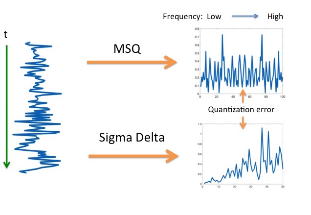
The main advantage of Sigma Delta quantization over MSQ is its adaptive usage of feedback information. The feedback information allows a quantizer to wisely allocate bits to efficiently store the entire signal. For example, adaptive quantization has been known to be extremely efficient for the class of slowly varying signals [15]. Intuitively speaking, this is because adaptive quantizers can push most quantization errors to the high-frequency region, known as the noise-shaping effect [14, 3, 11], so that the low-frequency region where the slowly varying signals reside are relatively clean. As displayed in Figure 1, via a comparison with MSQ, we see that with the same random sequence as input, the error of MSQ is uniformly distributed across the entire spectrum, while that of Sigma Delta quantization is mostly concentrated in the high-frequency regions. Mathematically speaking, the noise shaping effect is a direct consequence of the definition of Sigma Delta quantization. Notice that the first-order Sigma Delta quantization (1.2) has an equivalent matrix form of
where is the quantization step size in (1.1) and is the finite difference matrix. This is saying that the quantization error is in the set , which is the -ball with radius linearly transformed by the matrix . Likewise, for the -order quantization (), we have
which means that the quantization error lies in the -ball linearly transformed by .
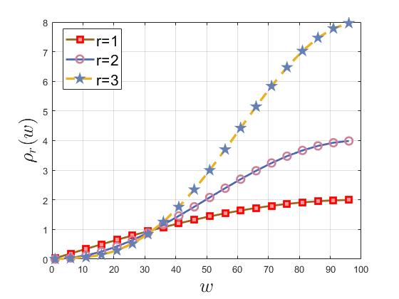
This is to say that, along each singular vector direction of , a scaling by the corresponding singular value is applied to the -ball. We have known from [22] that the singular vectors of are almost aligned with the Fourier basis, and the singular values of increase with frequencies. Therefore, when computing for some in the -ball, the low-frequency components of would be compressed more than the high-frequency ones as they correspond to smaller singular values of . One can numerically verify this unbalanced scaling by for various values of . Specifically, we hit by sinusoids with various frequencies and compute the ratio
where , with , are uniform samples in . Figure 2 is a plot of when setting , , and . One can see that sinusoids with lower frequencies have less energy left after hitting with , especially when the order of quantization is large, thus confirming the assertion that components with lower frequencies are cleaner under Sigma Delta quantization.
Since Sigma Delta quantization introduces smaller errors for low-frequency components, it was primarily used for quantizing low-frequency (i.e., slowly-varying) vectors. For instance, the sequence of dense (over Nyquist-rate) samples of audio signals can be deemed as low-frequency vectors, for which the superior performance of Sigma Delta quantization has been shown in [15, 21]. Images, on the other hand, are not purely made of low-frequencies. Because sharp edges, as important components of images, have slowly decaying Fourier coefficients. Therefore it is not obvious whether applying Sigma Delta quantization to images is beneficial.
1.4 A quick review of image quantization
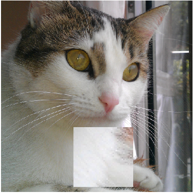
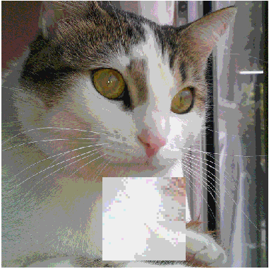
Despite the importance of quantization in image acquisition, the non-adaptive MSQ is thus far the state-of-the-art method in digital imaging devices. The major drawback of MSQ is that when the bit-depth (i.e., the number of bits used to represent each pixel) is small, it has a color-banding artifact: similar colors merge into one, causing fake contours and plateaus in the quantized image (see (B) of Figure 3). A famous technique called dithering [35, 39] reduces color-banding by randomly perturbing the pixel values (e.g., adding random noise) before quantization. It then breaks artificial contour patterns into less harmful random noises. However, this random noise is still quite visible as shown in (C) of Figure 3. A more fundamental issue is that dithering only randomizes the quantization error instead of reducing it. The same amount of error still exists in the quantized image and will manifest itself in other ways.
Another method to avoid color-banding is digital half-toning, proposed in the context of binary printing, where pixel values are converted to 0 or 1, leading to a possibly severe color-banding artifact. To mitigate it, the digital half-toning was proposed based on the ideas of sequential pixel quantization and error diffusion. Error diffusion means the quantization error of the current pixel will spread out to its neighbors to compensate for the overall under/over-shooting. The rate of spreading is set to empirical values that minimize the overall quantization error of an entire image class. Error diffusion works under a similar assumption as the Sigma Delta quantization that the image intensity varies slowly and smoothly. In a sense, it trades color-richness with spatial resolution. Similar to dithering, error diffusion does not reduce the overall noise but only redistributes it.
1.5 Contribution
From the discussion in Section 1.4, we see that both dithering and digital halftoning are only redistributing the quantization error instead of compressing it. In contrast, the method we introduce in this paper achieves a real reduction of the quantization error upon that of MSQ. Explicitly, suppose is the total number of pixels and is the number of pixels representing curve discontinuities (e.g., edges) in the image, then our method reduces the quantization error from to . This is achieved by combining Sigma Delta quantization with an optimization-based reconstruction algorithm. We observe in the numerical experiments that both the low and high frequency errors are reduced.
Due to the use of the total variation norm in the decoding optimization, our result is closely related to super-resolution theory [9, 10, 30] in compressed sensing, where it has been demonstrated that a sparse signal can be super-resolved using an -norm minimization if all the spikes in the signal are well-separated. We stress that the error reduction we achieve for image quantization does not require the edges of the image to satisfy this separation condition, although if the separation condition is met, a further error reduction can be achieved.
Besides Sigma Delta quantization, there exist other adaptive encoders (e.g., Beta encoder [11, 12, 13, 23]). These encoders had been used successfully on 1D audio signals to improve the bit-rate-distortion over MSQ, but none of them has been used for images. One major reason is that previous analyses (e.g., [3, 40, 5, 15, 16]) all indicated that these adaptive schemes can only compress low-frequency noise by sacrificing the high-frequency accuracy. While this might be a good idea for audio signals, one does not want to make such a sacrifice when it comes to images. In this paper, we demonstrate that a carefully designed decoder can help retain the high-frequency information while compressing the low-frequency noise. Therefore, the overall result outperforms MSQ. We only consider Sigma Delta quantization in this paper and leave the study of other adaptive quantizers on images as future work.
Unlike previous works on quantization under frame or compressed sensing measurements (see, e.g., [34, 6, 27, 5, 22, 28, 3, 29, 20, 2, 18, 26, 32, 33, 24, 17, 18, 19]), where samples are assumed to be taken by random Gaussian/sub-Gaussian or Fourier measurements, here we allow a direct quantization on each pixel and therefore ensure maximal practicality.
Another contribution of the work is an extension of Sigma Delta quantization to higher dimensions. We found that the proposed two-dimensional Sigma Delta quantization can effectively reduce the artifacts in the reconstruction while being as fast as the 1D quantization.
2 Proposed Method
We propose an adaptive quantization framework for natural images. Given an input image, the quantization workflow involves:
-
•
segmentation: divide the image into columns or rectangular patches. Here and throughout the paper, we use the term “patch” to refer to the set of image pixels restricted to a rectangular window of a certain size;
-
•
quantization: use the existing 1D quantization in the literature to quantize each column in parallel or use the proposed 2D quantization (in Section 2.2) to quantize each rectangular patch in parallel;
-
•
reconstruction: run the proposed decoding algorithms (Section 3) to restore the columns or patches and stack them into the final reconstructed image.
2.1 The encoders
We consider two types of encoders/quantizers in this paper.
-
•
Encoder 1 (): 1D -order Sigma Delta quantization applied to each column of the image (i.e., column-by-column quantization);
-
•
Encoder 2 (): 2D -order Sigma Delta quantization applied to each patch of the image (i.e., patch-by-patch quantization).
An important question one may ask is the practicality of the proposed adaptive quantizers when used in commercial cameras. A natural concern is the waiting time. Unlike MSQ that quantizes each pixel in parallel, Sigma Delta quantization can only be performed sequentially, which seems to inevitably introduce extra waiting time. However, this is not the case as current cameras are already using sequential quantization architectures for consistency, energy, and size considerations. More specifically, in current cameras, to reduce the number of ADC (Analog to Digital Converters) and save energy, one column of pixels or the whole image are assigned to one ADC, which means the pixels in one column or those of the entire image need to wait in a queue to be quantized. This architecture is perfect for Sigma Delta quantization. The only minor change one needs to make is adding additional memory units to the circuit to store the state variables.
The structure of the rest of the paper is as follows. In Section 2.2, we introduce the proposed 2D Sigma Delta quantization along with some of its properties. In Section 2.3, we introduce three image models which are of interest to this paper. In Section 2.4, we present three decoders associated with each of the three image models and summarize the reconstruction accuracy. The main theorems containing the reconstruction error bounds and their derivations can be found in Section 3. In Section 5.2 of the appendix, we describe an efficient algorithm for solving the proposed optimization problems in the decoding process. Finally, in Section 4, we perform numerical experiments to verify the conclusion of the theorems and to provide more evidence of the efficacy of the proposed method in real applications.
2.2 High dimensional Sigma Delta quantization
Although we can apply 1D quantization column by column to an image, it is likely to create discontinuities along the horizontal direction. As images are two-dimensional arrays, a two-dimensional quantization scheme is needed in maintaining the overall continuity. For this purpose, we propose the first high-dimensional Sigma Delta quantization.
Recall that in a nutshell, the existing 1D first-order Sigma Delta quantization : ( is the alphabet) is defined by constructing for any , two vectors (the quantization) and (the state variable) of the same length as and obeying
-
(A1)
(boundedness/stability): , for some constant independent of ;
-
(A2)
(adaptivity): with , , being the component of the vectors , and , respectively;
-
(A3)
(causality): only depends on the history of the input , that is , for any and some function .
We now extend these conditions to two dimensions, and the extensions to higher dimensions are similar. A 2D Sigma Delta quantization is well-defined and denoted as : , if we can construct for any input image , two matrices and satisfying the following three conditions:
-
(A1’)
(boundedness/stability): ( denotes the entry-wise maximal magnitude of a matrix) for some constant ;
-
(A2’)
(adaptivity): which has a matrix representation of ; and
-
(A3’)
(causality): ) for some function .
Provided that the quantization alphabet is large enough, one can show that a pair of and that satisfies (A1’)-(A3’) can be constructed through the recursive formula
| (2.1) | ||||
where . When or , the first row and column can be initialized using the 1D quantization. In the extreme case of -bit quantization, the existence of and obeying (A1’)-(A3’) for all is unknown, and we leave this as further work. Here we focus on the case when the bit-depth is greater than or equal to two. We first show in Proposition 2.1 that a stable 2D Sigma Delta quantization exists and then in Proposition 2.2 that the uniform alphabet with a certain step-size has the optimal stability among all alphabets of the same bit-depth.
Proposition 2.1.
For a given pair of real values with and a bit-depth , there exists an alphabet such that for any 2D array , the and generated by (2.1) satisfy (A1’)-(A3’) with .
Proof.
Let , and create the alphabet as
Then . Now we use the second principle of induction to show that generated by (2.1) satisfies .
-
•
Induction hypothesis: if for all the pairs such that , then .
-
•
Base case: .
-
•
Induction step: if , then by the induction hypothesis, we have , thus . The same reasoning follows when .
If , by the induction hypothesis, we have . Hence .
∎
The next proposition shows that the stability constant associated with the uniform alphabet
in Proposition 2.1 is optimal. We provide the proof of Proposition 2.2 in Section 5.1 of the appendix.
Proposition 2.2.
For a fixed bit-depth , the alphabet for the 2D quantization given in Proposition 2.1 is optimal, in the sense that if is the stability constant of any other -bit alphabet (not necessarily equally spaced), then it is necessary that , where is the stability constant of .
Remark 2.3.
The computational complexity of the 2D quantization scheme (2.1) is . However, noticing that for a fixed , all with (the points on the anti-diagonal) can be computed in parallel, therefore the quantization time can be reduced to .
Remark 2.4.
The matrix representation of (2.1) is
It is straightforward to extend this first-order quantization to higher orders. If , the -order quantization obeys the matrix form recursive formula
2.3 Notation and Assumptions
Throughout, we assume that the image to be quantized is an matrix. Everything discussed in the paper can be easily generalized to rectangular matrices. We write , where denote its columns and and the rows. Let be the difference matrix with s on the diagonal and s on the sub-diagonal and be the circulant difference matrix with an extra -1 at the upper right corner. For vectors, we denote by the -norm and by the -norm. For a continuous function , we denote by its -norm. For matrices, stands for the maximum absolute entry, and is the entry-wise -norm, i.e., . For both vectors and matrices, is the number of nonzero entries. Also, () denotes the unnormalized DFT matrix. We use to represent the row of corresponding to frequency , which can also be recognized as the operator that maps a vector to its discrete Fourier coefficient at frequency . We use for the matrix containing the rows of associated with frequencies in the set , and denote . In addition, stands for the circulant convolution operator between two vectors, is the 1D torus, and means that there exists some constant independent of , such that for all .
Our general assumption is that images have nearly sparse gradients. To be more precise, we consider three classes of images satisfying one of the three assumptions below.
Assumption 2.1.
(Class 1: -order column-wise or row-wise sparsity condition) Suppose is an image, the columns or rows of are piece-wise constant or piece-wise linear. Explicitly, for or , there exists ,
If , the columns or rows of image are piece-wise constant, if , they are piece-wise linear.
Assumption 2.2.
(Class 2: -order 2D sparsity condition) Suppose is an image, both columns and rows in are piece-wise constant or piece-wise linear. Explicitly, for or , there exists , such that
Assumption 2.3.
(Class 3: -order minimum separation condition) satisfies Assumption 2.1. In addition, the -order differences of each column or row of satisfy the -minimum separation condition defined below for some small integer . Explicitly, this means that for or , with or with satisfy the -minimum separation condition. Note that here is the circulant difference matrix.
Definition 2.1.
(-minimum separation condition) For a vector , let be the support of . We say that satisfies the -minimum separation condition if
| (2.2) |
where is the wrap-around distance on the set .
In addition, following [30], we use the definition for the space of trigonometric polynomials up to degree on the 1D torus , i.e.,
2.4 The proposed decoders and error bounds
For each image class, we will set the encoder to be either the or defined in Section 2.1, and let be the image of interest. The various decoders we shall propose for different classes of images will all be in the general form of
| (2.3) |
Here is 1 or 2 depending on whether the image is assumed to be (approximately) piece-wise constant or piece-wise linear, is some penalty that encourages sparsity in the gradients, is the order of Sigma Delta quantization, and is the feasibility constraint corresponding to a specific quantization scheme. Let be a solution to the general form (2.3), we shall obtain reconstruction error bounds of the following type
| (2.4) |
where , are the same as defined above (2.4), is the size of the image and is the step-size of the alphabet.
Now we specify what the and in (2.3) should be for each class of images and provide the associated error bound. Note that in Assumption 2.1 and Assumption 2.3, the images are allowed to be either row-wise sparse or column-wise sparse. Since their treatments are the same, from now on, we assume the images are column-wise sparse.
-
•
Class 1: satisfies Assumption 2.1 with order or and sparsity . We use the encoder proposed in Section 2.1 with order , and an alphabet with a step-size . We solve the following optimization problem for a reconstruction
(2.5) where is the maximum entry-wise absolute value. Theorem 3.1 below shows that the reconstruction error is
where is a universal constant.
- •
-
•
Class 3: satisfies Assumption 2.3 with order and sparsity . The encoder is with an alphabet spacing of (proposed in Section 2.1) and . Here we define a new alphabet with a smaller step-size to quantize the last entries of each column:
where , , and The total number of boundary bits is of order , which is negligible compared to the bits needed for the interior pixels. Since is finer than , the feasibility constraint is tighter at the last entries of each column:
where refers to the last rows of , and is the largest magnitude of the entries. Overall, we use the following optimization to obtain the reconstructed image :
(2.7) In Theorem 3.7, we obtain the following error bound
where is a universal constant and is the same as in Assumption 2.3. In the following, we discuss Class 1 in Section 3.1, Class 2 in Section 3.2, and Class 3 in Section 3.3.
3 Main theorems and their proofs
Without loss of generality, we assume the image has bounded pixel values, i.e., , and images satisfying Assumption 2.1 and Assumption 2.3 are column-wise sparse. The same results can be similarly obtained for row-wise sparse images.
3.1 Class 1: Images with no minimum separation
In this section, we consider Class 1, where the image satisfies Assumption 2.1 with , or for all the columns. We use the encoder that performs column-by-column quantization and use the decoder (2.5). Both the encoder and decoder can be decoupled into columns and run in parallel.
For each column , let be its -order Sigma Delta quantization, i.e., and take . For the simplicity of notation, we use and to represent and , respectively. The decoder (2.5) decouples into columns. For each column, it is
| (3.1) |
Since represents the -order difference of , the -norm here promotes sparsity of the gradients. The ball-constraint is a well-known feasibility constraint for Sigma Delta quantization (e.g., [37]).
The following theorem provides the error bound for this decoder.
Theorem 3.1.
For any satisfying with , and with . Let be a solution to (3.1), then
| (3.2) |
where is some absolute constant independent of the choice of .
Remark 3.2.
The error bound in Theorem 3.1 is for each column. Putting all columns together, we have
Remark 3.3.
For comparison, we specify the quantization error of MSQ and that of the vanilla Sigma Delta decoder. In MSQ, the quantization error for each pixel is . Since the pixels are quantized independently, the total quantization error of an image in the Frobenius norm is . Similarly, when using quantizers ( or ) but decoding with the following naive decoder,
the worse-case error is again . This indicates that the TV-norm penalty in the proposed decoder (3.1) is playing a key role in reducing the error to .
Theorem 3.4.
Let and . Let be a solution to (3.1), with , and , then for any integer , we have
| (3.3) |
where is the -tail of , i.e., . is some absolute constant independent of the signal .
3.1.1 Proof of Theorem 3.1 and Theorem 3.4
Proof of Theorem 3.1.
Denote . Assume the support set of is with cardinality and the complement of is . Since is a solution to (3.1), we have
which gives . We can then bound the -norm of as
| (3.4) |
where the last inequality is due to
(3.4) is equivalent to
| (3.5) |
In addition, we also have
| (3.6) |
(3.5), (3.6) above are bounds in -norm and -norm, respectively. Due to the duality, we can bound the reconstruction error as
This is equivalent to saying that . ∎
Proof of Theorem 3.4.
The proof follows a similar idea to Theorem 3.1. Assume that is the best -term approximation to , and assume the support of is . Since is a solution to (3.1), we have
Here we only used the triangle inequality. Applying to the left hand side of the above inequality and after some simplification, we obtain
This further implies
| (3.7) |
Following the same reasoning as in the proof of Theorem 3.1, we have
which when plugged into (3.7) gives us
| (3.8) |
This is saying that . ∎
3.2 Class 2: Decoding high-dimensional Sigma Delta quantized images
In this section, we consider Class 2, where the image satisfying Assumption 2.2 is associated with the encoder . For simplicity, we assume the patch number is 1 (there is only one patch identical to the original image) and . Results for more than one patches and/or follow the same argument. The theorem below establishes the error bound for 2D reconstruction of from its quantization using (2.6).
Theorem 3.5.
Similar to Theorem 3.4, we can extend Theorem 3.5 to images that does not satisfy Assumption 2.2. This extension follows the same idea as the one we used for Theorem 3.4 so its proof is omitted.
Theorem 3.6.
Let and let be a solution to (2.6) with . Then for any integer , we have
| (3.10) |
where for any matrix , denotes the -error between the vectorized and its best -term approximation.
Proof of Theorem 3.5.
Denote , , and denote by and the support sets of and , respectively. The corresponding complement sets are and . By Assumption 2.2, we have . Also notice that
which gives . Hence
Here the last inequality is due to , and
Then we have the following inequalities:
Similar to the proof of Theorem 3.1, the inequalities above lead to
which is (3.9). ∎
3.3 Class 3: Reconstruction of Images Meeting the Minimum Separation Condition
In this section, we consider Class 3, where the image satisfies Assumption 2.3, which is stronger than Assumption 2.1 in that jump discontinuities are not required to be separated. We hope that this extra assumption, when satisfied by an image, can lead to a reduction of the reconstruction error. Same as in Class 1, we use (column-by-column quantization) for encoding. The reason why we do not use is that the 2D minimum separation condition is not realistic for natural images.
For , its Sigma Delta quantization is . Again, we use and to replace and for simplicity. Then (2.7) reduces to
| (3.11) | ||||
There are two differences between this decoder and the decoder we used for Class 1: 1) Inside the -norm, this decoder uses (the circulant difference matrix) instead of . This is to ensure that the separation condition is well-defined at the boundary; and 2) In order for the separation assumption to improve the error bound of Class 1, we need to use a few more bits to encode the boundary pixels as explained in Sect. 2.4. The total number of boundary bits is of order , which is negligible compared to the bits needed for the interior pixels.
Theorem 3.7.
For the high order quantization, i.e., , assume and satisfies the -minimization separation condition with . Let be a solution to (3.11). Then for an arbitrary resolution , the following error bound holds:
| (3.12) |
Here is the projection onto the low-frequency range , i.e., with containing the rows of the DFT matrix with frequencies in .
Remark 3.8.
After applying the decoder (3.11) to each column, we put the reconstructed columns together to obtain the reconstructed image , the overall error bound in max-norm (entry-wise maximum magnitude) is then
Substituting with , we obtain
Remark 3.9.
3.3.1 Proof of Theorem 3.7
In order to prove Theorem 3.7, we perform the super-resolution analysis [9, 10, 30] under the Sigma Delta framework. We first need the following lemma.
Lemma 3.10.
For any feasible satisfying the constraints in (3.11), the following inequality holds:
Remark 3.11.
Substituting the in Lemma 3.10 by (the minimizer), we can see that the low-frequency error decreases as the order of the quantization increases.
Proof.
Denote . Recall that the discrete Fourier coefficient of at frequency is , where is the row vector with as its entry. Also recall that the projection operator in the target inequality is equivalent to the sum of the outer products of , divided by . For an arbitrary nonzero frequency , denote Then we have
Therefore is equivalent to a scaling of . Next, we show that is also close to a scaling of , which will yield a simple relation between and . Specifically, a direct calculation gives
Similarly, we have
More generally, for ,
Multiplying on both sides and rearranging the terms give,
Note that for , . Then the equation above holds for all integers with . Denote as the diagonal matrix with diagonal entries being , and let be the matrix consisting of with as its first to the rows, we obtain the matrix form of the previous equation
Here represents the all-one vector. Multiplying to both sides of the above equation and replacing with , we have
Note that . Hence , and the following error bound in -norm holds
| (3.13) | ||||
Here (3.3.1) is due to the feasibilities of and the true signal :
where stands for the last entries of . These two inequalities and the triangle inequality imply . From this last inequality, we further have for all , , which leads to (3.3.1). ∎
Denote the -order derivative of the reconstruction error by . For convenience of notation, we index the entries of from to , i.e., . We shall first show that is small, then using it, we prove that the overall reconstructing error is also small, where is the highest frequency we hope to super-resolve. To show that is small, we divide it into two parts, a part that contains elements within a neighborhood of some nonzero element of , and a part that contains the rest of the elements.
For satisfying the -minimum separation condition, suppose its support set is . Then can be viewed as samples on the discretized torus, . As in [30], we define
and
Then the following lemma shows that the energies of both parts of can be controlled.
Lemma 3.12.
[Discrete version of Proposition 2.3, [30]] If satisfies the -minimum separation condition, with the defined above, then there exists a constant such that the following holds
| (3.14) |
| (3.15) |
Proof.
Recall that is the support set of . Write with some , for Invoking Lemma 5.1 in Section 5.1 of the appendix, and taking , there exist defined on and constants such that
| (3.16) |
| (3.17) |
| (3.18) |
Denote for . Then we have
where the last inequality used (3.17) and (3.18). Rearranging the inequality, we obtain
| (3.19) |
Using to represent the -dimensional vector , we notice that . Also note that is a solution to (3.11), so it holds that
Rearranging the above inequality, we have
Then (3.19) becomes
Lemma 3.10 and Lemma 3.12 together ensure that is small. In the following, we show that this small further implies a small , which completes the proof of Theorem 3.7.
Proof of Theorem 3.7.
To start with, we consider a kernel that is an arbitrary function on the 1D torus . Define the discretization of by the boldface letter , that is, is the -dimensional vector with that contains samples of at the grid points . In what follows, the normal font always refers to the continuous kernel and the boldface refers to the discretization. We need to frequently take their infinity norms, denoted as and , respectively, and by definition, we have .
The proof contains two steps. In the first step, we bound for any general . In the second step, we pick a special to obtain the desired result.
For an arbitrary , by the definition of and the fact that and are periodic, it holds that
Hence,
| (3.20) | ||||
On the interval , we approximate with its first-order Taylor expansion around ,
where is some value between and . Inserting this into (3.20), we obtain
To bound the first term on the right hand side, we use an interpolation argument. Let such that and by Proposition 2.4 in [30], when , there exists a function such that
| (3.21) |
| (3.22) |
which gives
Here with . Below, we will use to represent the -dimensional vector . From (3.21) and (3.22), we obtain
Combining these results, we have
| (3.23) | ||||
where the last inequality used Lemma 3.12 and hides a constant. Next, we plug in a special kernel to to prove the theorem. For an arbitrary resolution , set , and denote by the discretized vector that contains samples of at . Then a direct calculation gives
We will bound the two terms on the right hand side separately. The second term is easy to bound due to the boundary constraint in (3.11) which forces the absolute value of the last rows in to be smaller than . Then we have
This gives . Next, we derive an upper bound on the first term .
Case I: TV order :
We construct an auxiliary function
Notice that
Hence satisfies the property
Also, since , we have Then the bound is equivalent to
where . Now we show that the infinity norm of is bounded by some constant for arbitrary and , then we can bound by (3.23). Since for , is -periodic, we have
Notice that for , we have , and then is of the same order as . Also for all , we have , which implies that . Then we can see that
This is saying that is close to . It is known that the latter is uniformly bounded by some constant smaller than ([1]) for arbitrary and , hence the former is also bounded. Therefore there exists some constant such that . Then we use Bernstein’s inequality for trigonometric sums [4] to obtain . Thus by (3.23) we have,
Case II: TV order :
Consider . Similar to Case I, we can show , for all , and . Then
In conclusion, for , we have the -norm error bound
which further gives
∎
4 Numerical simulation
In this section, we present the numerical simulation results of the proposed schemes on 1D synthetic signals as well as 2D natural and medical images. The specific algorithms that we have used to obtain these results will be discussed in Section 5.2 of the appendix.
We first define several terms. An RGB image is a composite of three gray-scale images, corresponding to the red, green, and blue channels. To evaluate the quality of the 1D reconstruction, we use the SNR (Signal-to-Noise Ratio) defined as
where is the true signal, and is the reconstructed one. For 2D images, we adopt the common evaluation metric PSNR (Peak Signal-to-Noise Ratio),
where and represent the clean and the reconstructed images, respectively, is the mean squared error between and , i.e., , and is the maximum possible pixel value of the image. For grayscale images, , and for RGB images, . In the following experiments, the unit for SNR and PSNR is decibel (dB).
4.1 1D synthetic signal
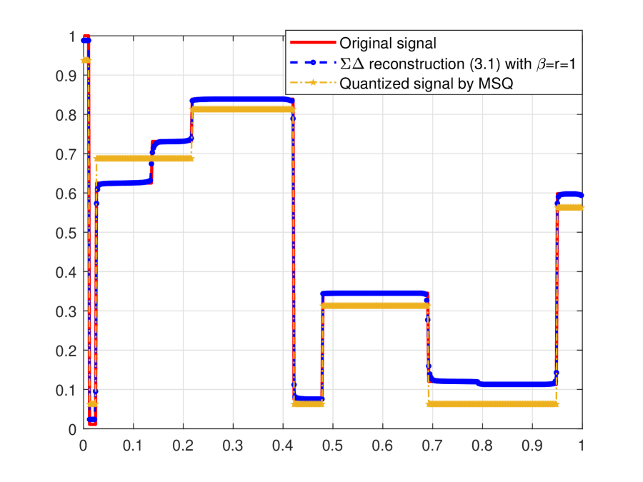
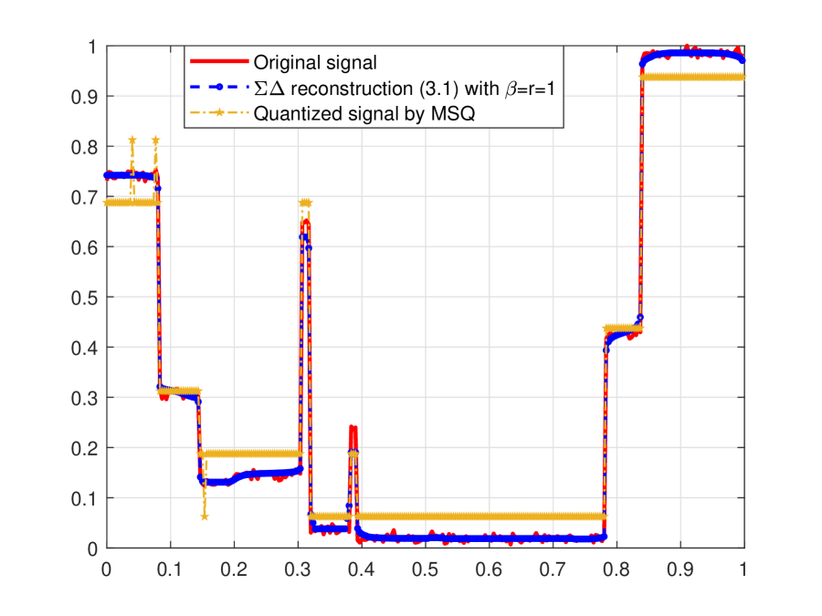
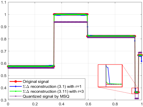
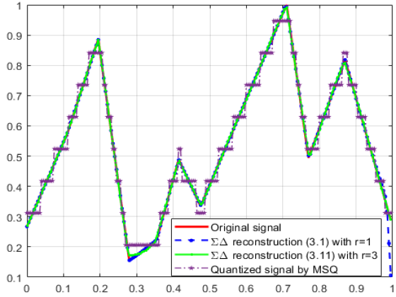
We design an experiment to confirm the advantage of the proposed methods over MSQ on 1D signals (representing columns of images) proved in Theorem 3.1. The signal to be quantized is piece-wise constant or piece-wise linear with random heights and slopes. Such signals satisfy our Assumption 2.1. We compare MSQ with Sigma Delta quantization coupled with the decoder (3.1). The result is displayed in Figure 4. We see from 4(a) that, with the same number of bits, the reconstructed signal using the -order quantization and decoder (3.1) is closer to the true signal than MSQ and better preserves the piece-wise constant structure. 4(b) shows a similar result for piece-wise linear signals. As real signals may be subject to noise, in 4(c), the reconstruction result under random Gaussian noise is shown. We see that the proposed encoder-decoder pair is pretty robust to noise.
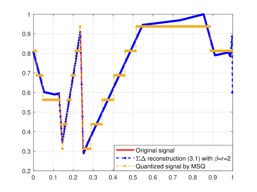
Our analysis in Section 3.3 predicted that, if the minimum separation condition is met, the quantization error can be further reduced through using a higher order quantization. This is confirmed in both (A) and (B) of Figure 5, where we see that the reconstructed signal from the -order quantization is indeed closer to the true signal than those from the first and second order quantization.
4.2 2D natural and medical images
In this section, we present numerical results for 2D images. We observe that the best performances are usually achieved when the TV order and the quantization order are both set to 1, perhaps because the test images fit our Class 2 model with better.
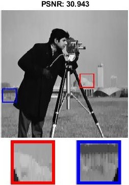
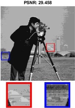
In the first example, on gray-scale images, we compare the 2D Sigma Delta quantization coupled with decoder (2.6) (sd2D), the 1D Sigma Delta quantization coupled with the decoder (2.5) (sd1D) and the MSQ quantization. For each quantizer, we employ its own optimal alphabet but require them to be subject to the same bit budget: 3 bits per pixel. In Figure 6, we see that in terms of visual quality (or the amount of artifact), (sd2D) is better than (sd1D) and much better than MSQ. In terms of the PSNR, (sd1D) is slightly better than (sd2D) and much better than MSQ.
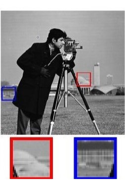
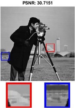

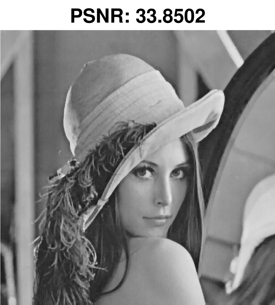
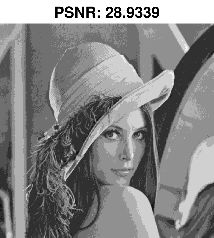


In the second experiment, on the test image Lena, we evaluate the effect of dividing the image into multiple rectangle patches in (sd2D), quantizing and reconstructing each patch individually. The process can be done in parallel, which significantly reduces the reconstruction time. As shown in Figure 7, there is no visible difference between the reconstruction by a single patch and that by multiple patches. In both cases, the images look more natural and closer to the original image than MSQ, especially around the face and shoulder areas.
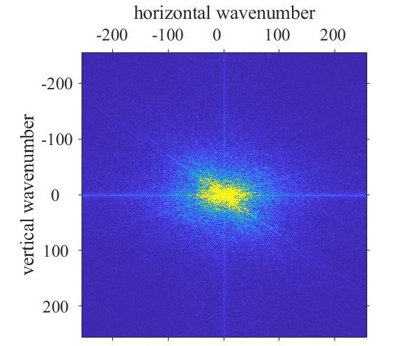
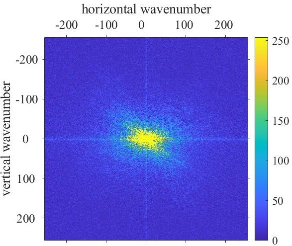
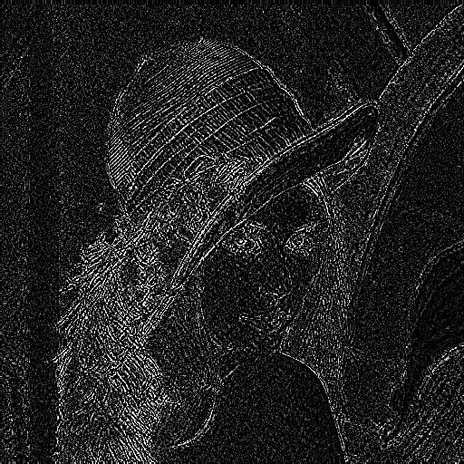
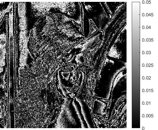
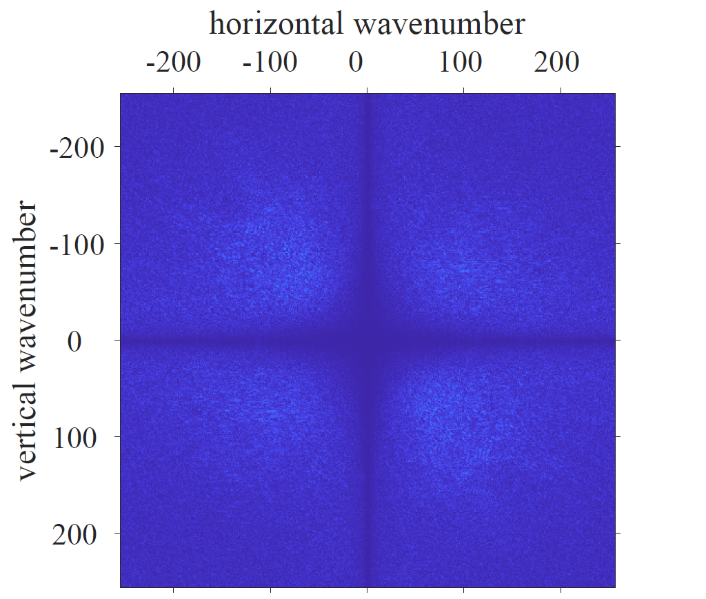
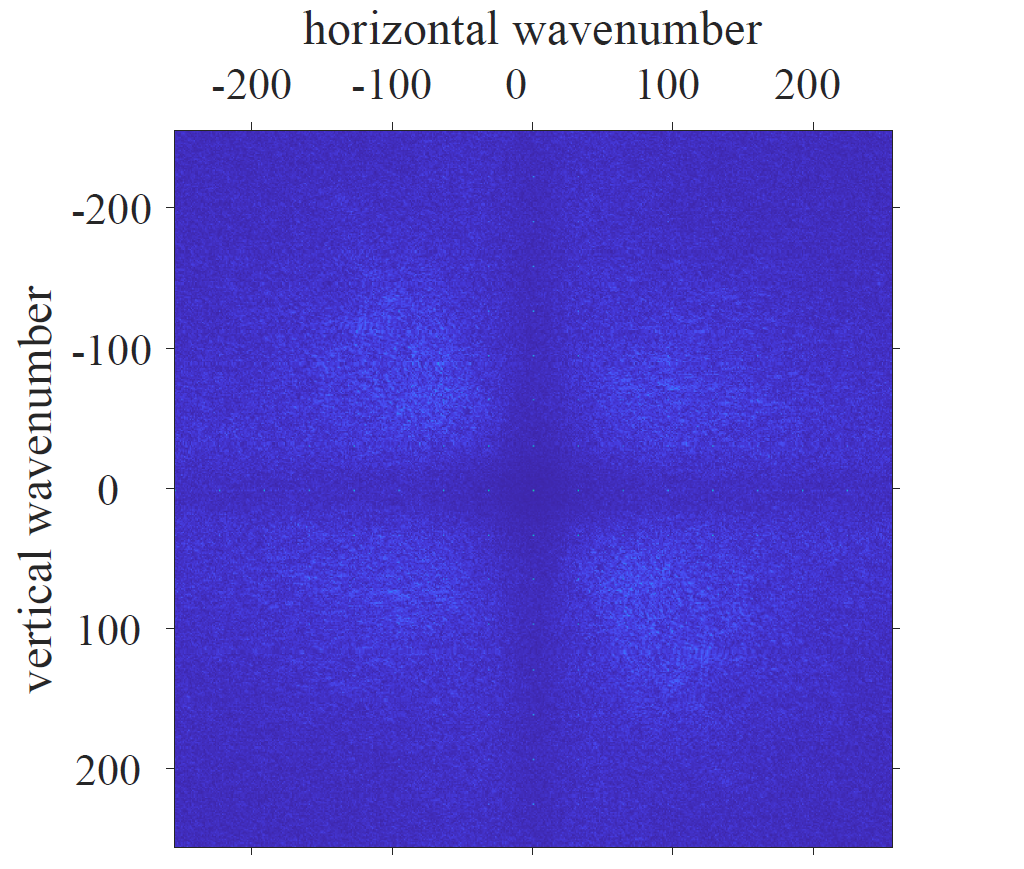
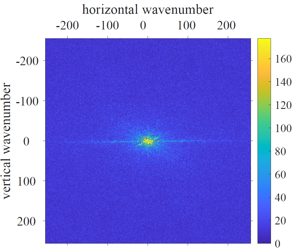
To further investigate where the improved PSNR of the Sigma Delta reconstructions comes from, we plotted in Figure 10 the absolute spectra of the three reconstructed images in Figure 8 as well as the absolute spectra of their residue images. The residue images (Figure 9) are obtained by taking differences between the reconstructed and the original images. From Figure 10, we see that as predicted, our decoders can indeed retain the high-frequency information while effectively compressing the low-frequency noise.
Next, we test the performances of the proposed decoders on RGB images.
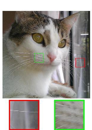
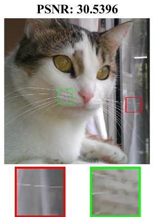
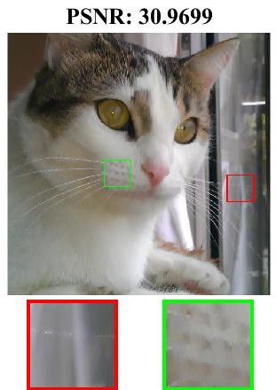
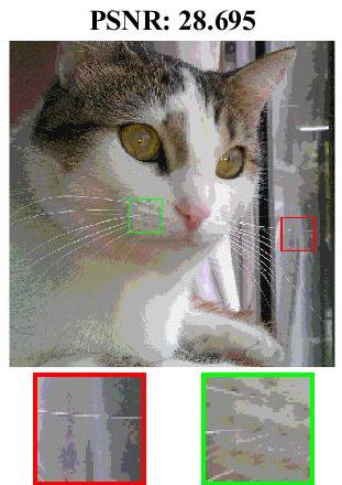
Figure 11 shows that compared with MSQ, the proposed reconstructions did a better job at preserving the original color and getting rid of the halos. Similar to the gray-scale image case (Figure 6), the 2D quantization introduced less horizontal artifact than the column-by-column quantization.
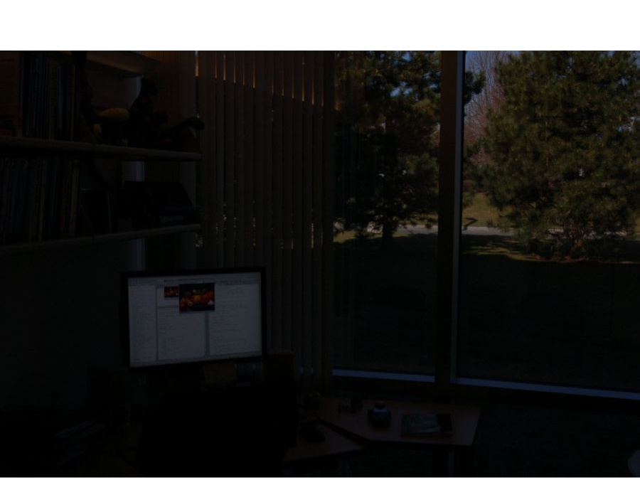
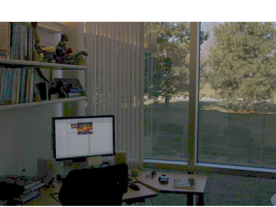
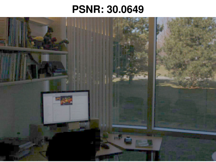
Next, we present an interesting result that shows the proposed scheme can greatly assist image acquisition under weak illuminations. When shooting in a dark environment or without an enough exposure time, the captured image will have a low overall pixel intensity (Figure 12(a)). We call such an image to have a low Dynamic Range (DR), meaning that the ratio between the maximum and minimum pixel intensities is small. Visually, it means that the contrast is small. A typical way to increase the contrast is through post-processing. For example, if we use the formula
| (4.1) |
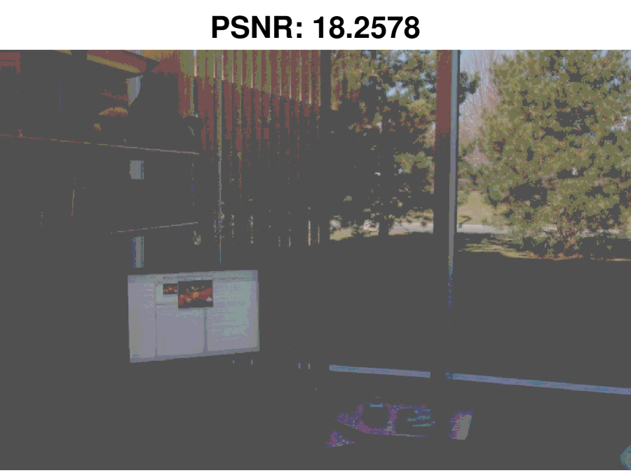
to adjust the brightness, Figure 12(a) is lightened up to Figure 12(b). However, in practice, since the brightness adjustment is a digital processing step, it has to be performed after quantization. If the quantization is performed using MSQ, because MSQ is not good at handling images with a low DR, the image quality becomes very poor (Figure 12(d)). With current commercial cameras, this (i.e., Figure 12(d)) is more or less what we could get for night scenes. In constrast, by replacing MSQ with the proposed Sigma Delta quantization, a significant improvement can be obtained under the same bit budget. As shown in Figure 12(c), hidden details in the dark scene are better revealed and less artifact is introduced. This promising performance under weak illuminations also carries over to the situations with extremely strong illuminations or with large and small intensity portions co-existing in one image.
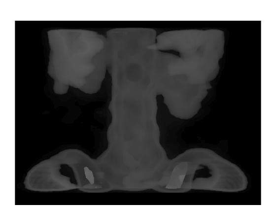
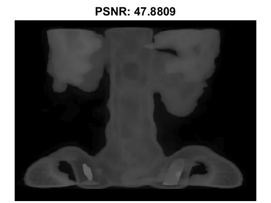

Last, we show that the proposed method is well-suited for medical imaging applications. Medical imaging has a higher tolerance for a longer decoding time, so there is no need to divide the image into patches. Also, in the previous experiments, methods were shown to be superior to MSQ at preserving the intensity variations among the pixels, which is crucial for medical images, as different intensity levels indicate different tissue types, that help doctors to detect the abnormally. In Figure 13, on the spine image, the 2D reconstruction from a 4-bit alphabet has almost no visual difference than the 8-bit original image, while MSQ quantization results in a larger distortion. This experiment indicates that the proposed quantization may be especially suitable for medical imaging.
5 Appendix
5.1 Proof of Proposition 2.2
Lemma 5.1.
[Lemma 2.4 [9]] Let be the 1-dimensional torus, suppose satisfies the -minimum separation condition, i.e., . Let be an arbitrary vector with Then there exists a low-frequency trigonometric polynomial
obeying the following properties:
with .
Proof of Proposition 2.2.
We proceed by contradiction, assume there exists a -bit alphabet whose stability constant is smaller than , i.e., . Let the alphabet be , with . Assume . Note that there is no restriction on the range of values of the alphabet, that is, it is possible that or . Also, denote the largest interval length in the alphabet within as , i.e., and define . The case is slightly easier than , so we first prove the result for .
For , we start with proving that the alphabet has at least two elements within , so is well defined. Notice that . If there is no or one between and , i.e., , then we can choose properly such that , which leads to a contradiction.
Next, we consider the following cases:
-
•
or . For this case, we have the following two sub-cases that are mutually exclusive: 1) and and 2) and . A closer look indicates that these two cases are exactly the same upon exchanging the roles of and . Hence without loss of generality, we assume 1) holds: and . Next, we specify the following possibilities:
(a) . Let be the largest interval in for some , i.e., . Choose , with small enough such as . This leads to , then , the quantization error
The second inequality used the assumption , and the third one used and . Then this contradicts the assumption .
(b) and . If , let with a sufficiently small as in (a), then . If , we can choose as in (a), then . In both cases, let , we have , and . The quantization error at is
This leads to a contradiction.
(c) and . If we choose with some small and , then . Since it holds for arbitrary small , we must have . This gives and , where the last inequality is due to the assumption so that . Same as in (a), we can choose properly and , such that , provided that is small enough. Then the quantization error at is
This also leads to a contradiction.
-
•
and . If we also have and , then we can easily choose a proper with quantization error at least , which leads to contradiction.
Therefore, without loss of generality, assume and . Similar to above, we specify the following sub-cases:
(d) . We first show that for an arbitrary constant , one can choose properly such that . If , set , then and . If , denote , then . Let be the largest interval in within for some , i.e., . Choose , then , we also have .
Hence whatever is, we can always obtain the quantization error
This leads to a contradiction. Here to see the first inequality, we consider the following sub-cases: i) if ; ii) if , take , then .
(e) and . Similar to (d), we first show that one can choose properly to make equal to an arbitrary constant between and . If , it follows the same reasoning as in (d), here we discuss the case when . If , let , then . If , denote , then , we specify the following sub-cases: i) if , let , then ; ii) if , let , and , then ; iii) if , let and , then .
Therefore, whatever is, the worst case quantization error can reach
This leads to a contradiction.
(f) and . We must have and . Then similar to (d), we can obtain the following quantization error
This also leads to a contradiction. We have exhausted all the cases for .
For the case , there are only elements in the alphabet with . Consider the case or , if there are at least two elements in that are within , the proof follows the same reasoning as . Here we discuss the case that and only one element of lies within , i.e., . In this case, we must have , and . For that is small enough, let , then . Hence , which leads to a contradiction.
Next, we discuss the two remaining cases when both and hold: and , which are the two cases that there is or elements in the alphabet between and , respectively.
-
•
. Without loss of generality, assume . Since , we must have . Combining these two inequalities we get , then . Choose some small and the first entries of as
Provided that is small enough, one can check that the first entries in are as follows
By assumption, we have , then for small enough , , this leads to a contradiction.
-
•
, we specify the following two cases:
(i) . Notice that we must have , so . We can choose and , then with a sufficiently small , and and , which leads to a contradiction.
(ii) , also notice that , then we can choose as follows
Provided that is small enough, the corresponding is
Since , then , which leads to a contradiction.
∎
5.2 Optimization
Although the proposed decoders (3.1), (2.6), (2.7) are standard convex optimization problems, off-the-shelf optimization solvers do not converge in meaningful time due to the existence of the matrix , which is very ill-conditioned. In this section, we suggest a special implementation of the primal-dual algorithm to achieve a much shorter decoding time. For a grayscale image, the decoding process now takes about 1 minute on an Intel Core i7 CPU@2.2GHz 16GB RAM PC. The decoding time can be further shortened to several seconds by dividing the image into patches and implementing quantization and decoding in parallel.
Since the treatments for all the decoders are similar, we only discuss (3.1). For simplicity, consider the case when the TV order and the quantization order are both set to 1, (3.1) then reduces to
| (5.1) |
Let us start with writing out the Lagrangian dual of (5.1)
| (5.2) |
which is a special case of the general form
| (5.3) |
(5.3) can be solved by primal-dual algorithms such as Chambolle-Pock (Algorithm 1).
To apply Algorithm 1 to our problem, we compare corresponding terms in (5.3) and (5.2) and naturally recognize that , , , . Then
| (5.4) |
However, applying Algorithm 1 to this results in a very slow convergence, because it contains the matrix with a large condition number (of order ).
We propose to move the ill-conditioned matrix into the sub-problem (b) in Algorithm 2 via a change of variable , or . Then the primal-dual objective becomes
| (5.5) |
Recognize that this is equivalent to setting and in (5.3). With this special and , Algorithm 1 becomes the following Algorithm 2.
In Algorithm 2, the ill-conditioned matrix appears in the sub-problem (b), but it does not make (b) an ill-conditioned problem thanks to the existence of the extra quadratic term. We can then solve (b) using standard ADMM and solve (a) by writing out its closed-form solution.
References
- [1] Horst Alzer and Stamatis Koumandos. Sharp inequalities for trigonometric sums in two variables. Illinois J. Math., 48(3):887–907, 2004.
- [2] R. G. Baraniuk, S. Foucart, D. Needell, Y. Plan, and M. Wootters. Exponential decay of reconstruction error from binary measurements of sparse signals. IEEE Trans. Inform. Theory, 63(6):3368–3385, 2017.
- [3] J. J. Benedetto, A. M. Powell, and Ö. Yılmaz. Sigma-delta () quantization and finite frames. IEEE Trans. Inform. Theory, 52(5):1990–2005, 2006.
- [4] S. Bernstein. Sur l’ordre de la meilleure approximation des fonctions continues par des polynômes de degré donné, volume 4. Hayez, imprimeur des académies royales, 1912.
- [5] J. Blum, M. Lammers, A. M. Powell, and Ö. Yılmaz. Sobolev duals in frame theory and sigma-delta quantization. J. Fourier Anal. Appl., 16(3):365–381, 2010.
- [6] B. G. Bodmann and V. I. Paulsen. Frame paths and error bounds for sigma–delta quantization. Appl. Comput. Harmon. Anal., 22(2):176–197, 2007.
- [7] P. T. Boufounos and R.G. Baraniuk. Quantization of sparse representations. In 2007 Data Compression Conference (DCC’07), pages 378–378. IEEE, 2007.
- [8] P. T. Boufounos, L. Jacques, F. Krahmer, and R. Saab. Quantization and compressive sensing. In Compressed sensing and its applications, pages 193–237. Springer, 2015.
- [9] E. J. Candès and C. Fernandez-Granda. Super-resolution from noisy data. J. Fourier Anal. Appl., 19(6):1229–1254, 2013.
- [10] E. J. Candès and C. Fernandez-Granda. Towards a mathematical theory of super-resolution. Comm. Pure Appl. Math., 67(6):906–956, 2014.
- [11] E. Chou. Beta-duals of frames and applications to problems in quantization. PhD thesis, New York University, 2013.
- [12] E. Chou and C. S. Güntürk. Distributed noise-shaping quantization: I. Beta duals of finite frames and near-optimal quantization of random measurements. Constr. Approx., 44(1):1–22, 2016.
- [13] E. Chou and C. S. Güntürk. Distributed noise-shaping quantization: II. Classical frames. In Excursions in Harmonic Analysis, Volume 5, pages 179–198. Springer, 2017.
- [14] E. Chou, C. S. Güntürk, F. Krahmer, R. Saab, and Ö. Yılmaz. Noise-shaping quantization methods for frame-based and compressive sampling systems. In Sampling theory, a renaissance, pages 157–184. Springer, 2015.
- [15] I. Daubechies and R. DeVore. Approximating a bandlimited function using very coarsely quantized data: a family of stable sigma-delta modulators of arbitrary order. Ann. of Math., 158(2):679–710, 2003.
- [16] Percy Deift, Felix Krahmer, and C Sınan Güntürk. An optimal family of exponentially accurate one-bit sigma-delta quantization schemes. Comm. Pure Appl. Math., 64(7):883–919, 2011.
- [17] S. Dirksen, H. C. Jung, and H. Rauhut. One-bit compressed sensing with partial gaussian circulant matrices. Inf. Inference, 9(3):601–626, 2020.
- [18] S. Dirksen and A. Stollenwerk. Fast binary embeddings with gaussian circulant matrices: improved bounds. Discrete Comput. Geom., 60(3):599–626, 2018.
- [19] J. M. Feng, F. Krahmer, and R. Saab. Quantized compressed sensing for random circulant matrices. Appl. Comput. Harmon. Anal., 47(3):1014–1032, 2019.
- [20] V. K. Goyal, M. Vetterli, and N. T. Thao. Quantized overcomplete expansions in ir/sup n: analysis, synthesis, and algorithms. IEEE Trans. Inform. Theory, 44(1):16–31, 1998.
- [21] C. S. Güntürk. One-bit sigma-delta quantization with exponential accuracy. Comm. Pure Appl. Math., 56(11):1608–1630, 2003.
- [22] C. S. Güntürk, M. Lammers, A. M. Powell, R. Saab, and Ö. Yılmaz. Sobolev duals for random frames and sigma-delta quantization of compressed sensing measurements. Found. Comput. Math., 13(1):1–36, 2013.
- [23] C. S. Güntürk and W. Li. High-performance quantization for spectral super-resolution. In 2019 13th International conference on Sampling Theory and Applications (SampTA), pages 1–4. IEEE, 2019.
- [24] T. Huynh and R. Saab. Fast binary embeddings and quantized compressed sensing with structured matrices. Comm. Pure Appl. Math., 73(1):110–149, 2020.
- [25] H. Inose and Y. Yasuda. A unity bit coding method by negative feedback. Proceedings of the IEEE, 51(11):1524–1535, 1963.
- [26] L. Jacques, J. N. Laska, P. T. Boufounos, and R. G. Baraniuk. Robust 1-bit compressive sensing via binary stable embeddings of sparse vectors. IEEE Trans. Inform. Theory, 59(4):2082–2102, 2013.
- [27] F. Krahmer, R. Saab, and R. Ward. Root-exponential accuracy for coarse quantization of finite frame expansions. IEEE Trans. Inform. Theory, 58(2):1069 –1079, February 2012.
- [28] F. Krahmer, R. Saab, and Ö Yılmaz. Sigma–delta quantization of sub-gaussian frame expansions and its application to compressed sensing. Inf. Inference, 3(1):40–58, 2014.
- [29] M. Lammers, A. M. Powell, and Ö. Yılmaz. Alternative dual frames for digital-to-analog conversion in sigma–delta quantization. Adv. Comput. Math., 32(1):73, 2010.
- [30] W. Li. Elementary error estimates for super-resolution de-noising. Preprint, arXiv:1702.03021, 2017.
- [31] E. Lybrand and R. Saab. Quantization for low-rank matrix recovery. Inf. Inference, 8(1):161–180., 2019.
- [32] Y. Plan and R. Vershynin. Robust 1-bit compressed sensing and sparse logistic regression: A convex programming approach. IEEE Trans. Inform. Theory, 59(1):482–494, 2012.
- [33] Y. Plan and R. Vershynin. Dimension reduction by random hyperplane tessellations. Discrete Comput. Geom., 51(2):438–461, 2014.
- [34] A. M. Powell, R. Saab, and Ö. Yılmaz. Quantization and finite frames. In Finite frames, pages 267–302. Springer, 2013.
- [35] L. Roberts. Picture coding using pseudo-random noise. IRE Transactions on Information Theory, 8(2):145–154, 1962.
- [36] R. Saab, R. Wang, and Ö. Yılmaz. From compressed sensing to compressed bit-streams: practical encoders, tractable decoders. IEEE Trans. Inform. Theory, 64(9):6098–6114, 2017.
- [37] R. Saab, R. Wang, and Ö. Yılmaz. Quantization of compressive samples with stable and robust recovery. Appl. Comput. Harmon. Anal., 44(1):123–143, 2018.
- [38] R. Schreier and G. C. Temes. Understanding delta-sigma data converters, volume 74. IEEE press Piscataway, NJ, 2005.
- [39] L. Schuchman. Dither signals and their effect on quantization noise. IEEE Transactions on Communication Technology, 12(4):162–165, 1964.
- [40] R. Wang. Sigma delta quantization with harmonic frames and partial fourier ensembles. J. Fourier Anal. Appl., 24(6):1460–1490, 2018.