Beam-Domain Secret Key Generation for Multi-User Massive MIMO Networks

Abstract

Physical-layer key generation (PKG) in multi-user massive MIMO networks faces great challenges due to the large length of pilots and the high dimension of channel matrix. To tackle these problems, we propose a novel massive MIMO key generation scheme with pilot reuse based on the beam domain channel model and derive close-form expression of secret key rate. Specifically, we present two algorithms, i.e., beam-domain based channel probing (BCP) algorithm and interference neutralization based multi-user beam allocation (IMBA) algorithm for the purpose of channel dimension reduction and multi-user pilot reuse, respectively. Numerical results verify that the proposed PKG scheme can achieve the secret key rate that approximates the perfect case, and significantly reduce the dimension of the channel estimation and pilot overhead.

I Introduction

The fifth generation (5G) and beyond communication systems have been developing at an unprecedented speed to meet the requirement of high data rate and low latency. In the 5G networks, the random access from tons of devices makes traditional cryptographic key distribution and management very challenging. Under this background, the physical-layer key generation (PKG) has emerged as an alternative technique to establish the symmetric key for cryptographic applications [1]. PKG can generate time-varying key with a lightweight algorithm from the channel randomness. Thanks to the channel decorrelation property, there is no information leakage to eavesdroppers, when they are located half a wavelength away or more from legitimate users [2].

The 5G networks employ massive MIMO technology to support extremely high throughput and multi-user access. However, traditional pairwise PKG method is difficult to scale to the new scenario due to the high dimension of channel matrix caused by massive MIMO antennas and the huge number of orthogonal pilot overhead to distinguish multiple users [1]. Jiao et al. proposed to use new channel characteristics, i.e., virtual angle of arrival (AoA) and angle of departure (AoD), to generate a shared secret key for pairwise users in a massive MIMO system [3]. However, they only considered the PKG between two legitimate users. Generating secret keys between a base station and multiple users has been a largely under explored domain [4]. Several work studied the group PKG protocols, where all users in the group negotiate a common key based on their channel estimates. But the majority of them still perform channel probing in a pairwise manner, resulting in an extremely large overhead and low efficiency. Hence, those works related to PKG among multiple nodes through the optimization of probing rates at individual node pair and channel probing schedule do not scale in this context. Exceptionally, Zhang et al. designed a multi-user key generation protocol by leveraging the multi-user access of OFDMA modulation, which is achieved by assigning non-overlapping subcarriers to different users [5]. However, no work has been devoted to exploiting the spatial diversity of massive MIMO to enable multi-user key generation.

In summary, it is still missing how to generate secret keys among multiple users in massive MIMO networks, which is tackled in this paper. The main contributions are as follows:

• We propose a channel dimension reduction approach by exploiting the spatial sparse property of the beam domain channel model. Employing this approach, legitimate users only need to estimate the effective channels at a few dominant beams, which allows us to reduce the dimension of channel estimation significantly.

• We propose a muti-user pilot reuse approach that can largely reduce the pilot overhead compared with using orthogonal signals. Furthermore, we present a novel algorithm to design the precoding and receiving matrices, with the purpose of achieving the perfect secret key rate.

• Numerical results verify that the approach can achieve the secret key rate that approximates the perfect case and significantly reduce the dimension of the channel estimation and the pilot overhead.

II Secret key generation with MU massive MIMO

II-A System Model and Problem Statement

This paper considers a narrow-band star topology network, where a base station (BS) simultaneously generates secret keys $\kappa=\{\kappa_{1},\kappa_{2},\cdots,\kappa_{K}\}$ with $K$ user terminals (UT), as shown in Fig. 1. The BS is equipped with $M$ antennas and the $k$-th UT is equipped with $N_{k}$ antennas. We consider the potential unintended hearing from other UTs and the active attacks are out of scope in this paper.

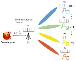
Figure 1: System model of multi-user secret key generation.

It is challenging for existing pairwise PKG approach to scale to multi-user massive MIMO scenarios due to two main reasons as follows.

1. High dimension of the channel matrix: The elements of the generated secret keys are highly auto-correlated due to the spatial correlation of the antennas, which must be reduced by decorrelation preprocessing algorithms. However, in a multi-user massive MIMO network, the high dimension of channel matrix makes it too complicated to perform the decorrelation preprocessing algorithms such as principal component analysis.

2. Large pilot overhead: The length of uplink pilots scales with the number of antennas as well as the number of UTs. Thus, in the massive MIMO network where the number of antennas is extremely large, it brings in large length of pilots to distinguish different users, while it is hard to accomplish channel probing within the coherence time in a time division duplex (TDD) system.

II-B Scheme Framework

The proposed framework for multi-user PKG is portrayed in Fig. 2. It contains four steps, namely channel probing, quantization, information reconciliation, and privacy amplification. The last three steps are similar with existing work summarized in [1], so this paper will focus on the first step, i.e., channel probing, which is relatively different from that in the point-to-point PKG. To address the two challenges mentioned above, the proposed channel probing scheme contains two novel parts, i.e., channel dimension reduction and multi-user pilot reuse.

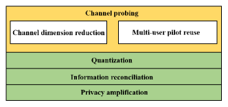
Figure 2: Framework of secret key generation scheme in the multi-user massive MIMO network.

1. Channel dimension reduction: In the massive MIMO channel matrix, only a few dominant elements contain the most relevant channel information. So we employ the beam domain channel model where the channel gains are concentrated in a few beams. In order to significantly reduce the dimension of the channel estimation, a beam-domain based channel probing (BCP) algorithm is proposed to obtain the CSI. This scheme will be presented in Section III.

2. Multi-user pilot reuse: In order to reduce the pilot overhead in massive MIMO network, we consider pilot reuse among the UTs, where different UTs transmit the identical pilot signals. With the purpose of mitigating the inter-user interference, we then present an interference neutralization based beam allocation algorithm (IMBA) to then proposed to design the precoding and receiving matrix. This algorithm will be discussed further in Section IV.

III Channel dimension reduction approach

III-A Beam-domain Channel Model

We consider a narrow-band multipath channel model. The downlink channel response of the $k$-th UT can be given as

$${\mathbf{H}}_{k}^{DL}=\sum_{p=1}^{N_{P}}{\mathbf{H}}_{k,p}^{DL} =\sum_{p=1}^{N_{P}}\alpha_{k,p}{\mathbf{a}}_{UT,k}(\theta_{k,p}){\mathbf{a}}^{H}_{BS}(\varphi_{k,p}).$$ (1)

where $N_{P}$ is the number of paths, ${\mathbf{H}}_{k,p}^{DL}$ is the downlink channel matrix associated with the $p$-th path of $k$-th UT [6], $\alpha_{k,p}$ is the complex gain of the $p$-th path, ${\mathbf{a}}_{UT,k}(\theta_{k,p})$ and ${\mathbf{a}}_{BS}(\varphi_{k,p})$ are the antenna array response vectors at the UT and BS with AoA $\theta_{k,p}$ and AoD $\varphi_{k,p}$, respectively. Specifically, under the uniform linear array (ULA) setup, these vectors are given by

$${\mathbf{a}}_{UT,k}(\theta_{k,p})=\frac{1}{\sqrt{N_{k}}}\left[1,e^{-j\Theta_{k,p}},\ldots,e^{-j(N_{k}-1)\Theta_{k,p}}\right]^{T}$$

$${\mathbf{a}}_{BS}(\varphi_{k,p})=\frac{1}{\sqrt{M}}\left[1,e^{-j\Phi_{k,p}},\ldots,e^{-j(M-1)\Phi_{k,p}}\right]^{T},$$ (2)

where $\Theta_{k,p}=\frac{2\pi}{\lambda}d\sin(\theta_{k,p})$, $\Phi_{k,p}=\frac{2\pi}{\lambda}d\sin(\varphi_{k,p})$, $\lambda$ is the wavelength, and $d$ is the distance between the adjacent antennas.

Beam domain model samples the original physical channel by two series of uniformly distributed beams/angles over $[0,2\pi]$, i.e., transmitting and receiving beams/angles. According to [7], the downlink beam domain channel response is

$${\tilde{\mathbf{H}}}_{k}^{DL}={\mathbf{A}}_{UT,k}^{H}{\mathbf{H}}_{k}^{DL}{\mathbf{A}}_{BS},$$ (3)

where ${\mathbf{A}}_{UT,k}=\left[{\mathbf{a}}_{UT,k}(\theta_{1}),{\mathbf{a}}_{UT,k}(\theta_{2}),\ldots,{\mathbf{a}}_{UT,k}(\theta_{N_{k}})\right]\in{\mathbb{C}}^{N_{k}\times N_{k}}$ and ${\mathbf{A}}_{BS}=\left[{\mathbf{a}}_{BS}(\varphi_{1}),{\mathbf{a}}_{BS}(\varphi_{2}),\ldots,{\mathbf{a}}_{BS}(\varphi_{M})\right]\in{\mathbb{C}}^{M\times M}$ are the sampling matrices at the $k$-th UT and the BS, respectively. The $(n,m)$-th element of ${\tilde{\mathbf{H}}}_{k}^{DL}$ represents the channel gains from AoD $\varphi_{m}$ to AoA $\theta_{n}$, where $\varphi_{m}$ and $\theta_{n}$ are the $m$-th and $n$-th sample angles, which satisfy that $\sin(\varphi_{m})=2m/M-1$ and $\sin(\theta_{n})=2n/N_{k}-1$.

Proposition 1

When the number of antennas grows to infinity, the $(n,m)$-th element of beam domain channel ${\tilde{\mathbf{H}}}_{k}^{DL}$ tends to [7]

$$\lim_{M,N_{k}\to\infty} \Big{(}[{\tilde{\mathbf{H}}}_{k}^{DL}]_{n,m}-\sum_{p=1}^{N_{P}}\alpha_{k,p}\delta(\theta_{k,p}-\arcsin(2n/N_{k}-1))$$

$$\times\delta(\varphi_{k,p}-\arcsin(2m/M-1))\Big{)}=0.$$ (4)

The beam domain channel covariance matrices ${\tilde{\mathbf{R}}}_{BS,k}={\mathbb{E}}\{({\tilde{\mathbf{H}}}_{k}^{DL})^{H}{\tilde{\mathbf{H}}}_{k}^{DL}\}$ and ${\tilde{\mathbf{R}}}_{UT,k}={\mathbb{E}}\{{\tilde{\mathbf{H}}}_{k}^{DL}({\tilde{\mathbf{H}}}_{k}^{DL})^{H}\}$ tend to diagonal matrices with the diagonal elements given by

$$\lim_{M\to\infty}[{\tilde{\mathbf{R}}}_{BS,k}]_{m,m}-\sum_{p=1}^{N_{P}}|\alpha_{k,p}|^{2}\delta(\varphi_{k,p}-\arcsin(2m/M-1))=0,$$

$$\lim_{N_{k}\to\infty}[{\tilde{\mathbf{R}}}_{UT,k}]_{n,n}-\sum_{p=1}^{N_{P}}|\alpha_{k,p}|^{2}\delta(\theta_{k,p}-\arcsin(2n/N_{k}-1))=0.$$

Remark 1

For each $n$ and $m$, there is at most one path $p$ simultaneously satisfying $\theta_{k,p}=\arcsin(2n/N_{k}-1)$ and $\varphi_{k,p}=\arcsin(2m/M-1)$, which means that different elements represent channel gains corresponding to different AoAs and AoDs. With a large (but finite) number of antennas, ${\tilde{\mathbf{H}}}_{k}^{DL}$ is a very sparse matrix with $N_{P}$ dominant elements corresponding to the paths. Moreover, these elements become independent with each other as long as these paths are independent. The $m$-th diagonal element in ${\tilde{\mathbf{R}}}_{BS,k}$ represents the channel gains of the $m$-th transmit beam ($\varphi_{k,p}=\arcsin(2m/M-1)$), and the $n$-th diagonal element in ${\tilde{\mathbf{R}}}_{UT,k}$ represents the channel gains of the $n$-th receive beam ($\theta_{k,p}=\arcsin(2n/N-1)$).

III-B The BCP Algorithm

In this section, we assume the precoding and receiving matrices have been provided, the algorithm of designing these matrices will be presented later in Section V.

In this stage, BS and UTs probe the channel alternatively and employ the precoding and receiving matrix to construct the reciprocal channel characteristics. Firstly, the BS transmits the downlink pilot signals by the precoding matrix ${\mathbf{P}}$ and UTs preprocess the received signals by the receiving matrix ${\mathbf{C}}^{H}$ to obtain the reciprocal channel parameters. Next, each UT employs the matrix ${\mathbf{C}}^{*}$ to transmit the pilot signals. The BS utilizes the matrix ${\mathbf{P}}^{T}$ to preprocess the received signals and estimate the effective channel.

Based on the analysis above, we propose a BCP algorithm, which is illustrated in Algorithm 1.

III-C Signal Presentation

In the downlink transmission, define the downlink pilot from BS to UT $k$ within $T_{D}$ time slots as ${\mathbf{S}}_{k}^{DL}\in{\mathbb{C}}^{M_{e}\times T_{D}}$, where $M_{e}$ is the dimension of the effective channel at the BS. To estimate the perfect CSI, the pilot signals of each UT are orthogonal. Based on the BCP algorithm, the downlink CSI estimated at UT $k$ side is

$$\!\!\!\!{\mathbf{Z}}_{k}^{DL}={\mathbf{C}}_{k}^{H}{\mathbf{H}}_{k}^{DL}\!\sum_{k^{\prime}}{\mathbf{P}}_{k^{\prime}}{\mathbf{S}}_{k^{\prime}}^{DL}({\mathbf{S}}_{k}^{DL})^{H}+{\mathbf{C}}_{k}^{H}{\mathbf{N}}_{k}({\mathbf{S}}_{k}^{DL})^{H}.$$ (6)

In the uplink transmission, define the pilot transmitted by UT $k$ within $T_{U}$ time slot as ${\mathbf{S}}_{k}^{UL}\in{\mathbb{C}}^{N_{e}\times T_{U}}$, which satisfies ${\mathbf{S}}_{k^{\prime}}^{UL}({\mathbf{S}}^{UL}_{k})^{H}={\mathbf{I}}$. Employing the BCP algorithm, the estimated uplink CSI of UT $k$ can be expressed as

$${\mathbf{Z}}_{k}^{UL}={\mathbf{P}}_{k}^{T}\sum_{k^{\prime}}{\mathbf{H}}_{k^{\prime}}^{UL}{\mathbf{C}}_{k^{\prime}}^{*}{\mathbf{S}}_{k^{\prime}}^{UL}({\mathbf{S}}^{UL}_{k})^{H}+{\mathbf{P}}_{k}^{T}{\mathbf{N}}({\mathbf{S}}^{UL}_{k})^{H}.$$ (7)

Algorithm 1 BCP algorithm.

1:${\mathbf{P}}_{k}$ and ${\mathbf{C}}_{k}$

2:${\mathbf{z}}_{k}^{UL}$ and ${\mathbf{z}}_{k}^{DL}$

3:In the downlink:

4:At the BS side:

5:for $k=1:K$ do

6:     Multiply the downlink pilot signals ${\mathbf{S}}_{k}^{DL}$ to UT $k$ by the precoding matrix ${\mathbf{P}}_{k}$ .

7:end for

8:Transmit the summation of all processed signals to UTs.

9:At the UT side:

10:for $k=1:K$ do

11:     UT $k$ multiplies received signal by the receiving matrix ${\mathbf{C}}_{k}^{H}$ and employ the LS estimation to estimate the downlink CSI ${\mathbf{Z}}_{k}^{DL}$.

12:     Vectorize the estimated effective channel matrices ${\mathbf{Z}}_{k}^{DL}$ as ${\mathbf{z}}_{k}^{DL}={\rm{vec}}({\mathbf{Z}}_{k}^{DL})$

13:end for

14:In the uplink:

15:At the UT side:

16:for $k=1:K$ do

17:     Multiply the uplink pilot signals ${\mathbf{S}}_{k}^{UL}$ to the BS by the matrix ${\mathbf{C}}_{k}^{*}$.

18:     Transmit the summation of all processed signals to the BS.

19:end for

20:At the BS side:

21:for $k=1:K$ do

22:     Multiply received signal by the matrix ${\mathbf{P}}_{k}^{T}$ and employ the LS estimation to estimate the uplink CSI ${\mathbf{Z}}_{k}^{UL}$.

23:     Vectorize the estimated effective channel matrices ${\mathbf{Z}}_{k}^{UL}$ as ${\mathbf{z}}_{k}^{UL}={\rm{vec}}({\mathbf{Z}}_{k}^{UL})$

24:end for

Remark 2

In the uplink and downlink transmissions, the BS and UTs vectorize the estimated effective channel matrices as ${\mathbf{z}}_{k}^{DL}={\rm{vec}}({\mathbf{Z}}_{k}^{DL})$ and ${\mathbf{z}}_{k}^{UL}={\rm{vec}}(({\mathbf{Z}}_{k}^{UL})^{T})$ to generate the secret key. As the uplink and downlink channels are reciprocal, the downlink channel ${\mathbf{H}}_{k}^{DL}$ is denoted as ${\mathbf{H}}_{k}$, and the uplink channel is ${\mathbf{H}}_{k}^{UL}=({\mathbf{H}}_{k})^{T}$. The reciprocal component between the BS and UT $k$ is ${\mathbf{C}}_{k}^{H}{\mathbf{H}}_{k}{\mathbf{P}}_{k}$ with a small dimension of $N_{e}\times M_{e}$. In this way, the dimension of channel characteristics is reduced by $\eta=\frac{M\times N_{k}}{N_{e}\times M_{e}}$ times. The dimensions of $M_{e}$ and $N_{e}$ are very small compared with the number of antennas, therefore the dimension can be significantly reduced.

III-D Secret Key Rate

This paper considers the condition that the beam domain channel between one UT and the BS is independent of that between one UT and another UT. Thus, the secret key rate is the minimum mutual information between ${\mathbf{z}}_{k}^{DL}$ and ${\mathbf{z}}_{k}^{UL}$, which can be expressed as $I_{k}=I({\mathbf{z}}_{k}^{DL};{\mathbf{z}}_{k}^{UL})$. Denote the precoding and receiving matrices in the beam domain as ${\tilde{\mathbf{P}}}_{k}={\mathbf{A}}_{BS}^{H}{\mathbf{P}}_{k}$ and ${\tilde{\mathbf{C}}}_{k}={\mathbf{A}}_{UT,k}^{H}{\mathbf{C}}_{k}$, respectively. Let ${\mathbf{V}}_{k}=\hbox{\boldmath$\Lambda$}_{k}^{1/2}\Big{(}\sum_{k^{\prime}}({\tilde{\mathbf{P}}}_{k^{\prime}})^{T}\otimes{\tilde{\mathbf{C}}}_{k}^{H}\Big{)}^{H}$ and ${\mathbf{V}}_{kk^{\prime}}=\hbox{\boldmath$\Lambda$}_{k^{\prime}}^{1/2}\Big{(}{\tilde{\mathbf{P}}}^{T}_{k}\otimes{\tilde{\mathbf{C}}}^{H}_{k^{\prime}}\Big{)}^{H}$, where $\hbox{\boldmath$\Lambda$}_{k}={\mathbb{E}}\{{\rm{vec}}({\tilde{\mathbf{H}}}_{k}){\rm{vec}}({\tilde{\mathbf{H}}}_{k})^{H}\}$ is the full correlation of the beam domain channel.

Theorem 1

When the channel of different UTs are independent, according to [7], we can compute the secret key rate of UT $k$ as

$$I_{k}=\!-\log\!\det\!\Bigg{(}\!{\mathbf{I}}-{\mathbf{V}}_{kk}\!\left(\!\sum_{k^{\prime}}{\mathbf{V}}_{kk^{\prime}}^{H}{\mathbf{V}}_{kk^{\prime}}\!+\!\Big{(}{\mathbf{P}}^{T}_{k}{\mathbf{P}}^{*}_{k}\otimes{\mathbf{I}}_{T_{U}}\!\Big{)}\!\!\right)^{-1}$$

$$\quad\times{\mathbf{V}}_{kk}^{H}{\mathbf{V}}_{k}\left({\mathbf{V}}_{k}^{H}{\mathbf{V}}_{k}+{\mathbf{I}}_{T_{D}}\otimes{\mathbf{C}}_{k}^{H}{\mathbf{C}}_{k}\right)^{-1}{\mathbf{V}}_{k}^{H}\Bigg{)}.$$ (8)

Proof:

See Appendix A. ∎

IV Multi-user pilot reuse approach

IV-A Pilot Reuse for Multi-users

According to (1), when the pilot signals of each UT are orthogonal, there is no inter-user interference and the estimated CSI achieves the perfect case. The pilot overhead is defined as the length of the total pilot signals. For traditional approach using the orthogonal pilot, the pilot overhead is given by

$$T_{TA}=M+\sum\limits_{k=1}^{K}{{N_{k}}}.$$ (9)

However, as $T_{TA}$ scales with the number of antennas and users, the overhead of orthogonal signals is extremely large in the multi-user massive MIMO network. Therefore, we consider the key generation scheme under the pilot reuse case, where different UTs transmit the identical pilot signals. In the pilot reuse case, the pilot overhead is reduced to

$$T_{PA}={M_{e}}+{N_{e}}.$$ (10)

Since pilot reuse results in interference between UTs and reduces secret key rate, it is necessary to mitigate the interference.

The interference neutralization approach can be employed to reduce the interference, i.e., for arbitrary matrix ${\tilde{\mathbf{C}}}_{k^{\prime}}$ ($k^{\prime}\neq k$), the precoding matrix ${\tilde{\mathbf{P}}}_{k}$ satisfies

$$({\tilde{\mathbf{P}}}_{k}^{T}\otimes{\tilde{\mathbf{C}}}_{k^{\prime}}^{H})\hbox{\boldmath$\Lambda$}_{k^{\prime}}={\bf 0},\quad k^{\prime}\neq k.$$ (11)

When the channel beams of different users are non-overlapping, we have

$${\tilde{\mathbf{P}}}_{k}^{H}{\tilde{\mathbf{R}}}_{BS,k^{\prime}}={\bf 0},\quad k^{\prime}\neq k.$$ (12)

The constraint of interference neutralization approach can always be satisfied under this case.

In order to mitigate the interference, the precoding and receiving matrices must satisfy the interference neutralization constraint. Therefore, a novel algorithm will be presented to help design these matrices.

IV-B The IMBA Algorithm

Referring to Proposition 1, as the number of antennas tends to infinity, different elements of the beam domain channel matrix ${\tilde{\mathbf{H}}}_{k}$ represent the channel gains from different AoDs to different AoAs, which indicates that the channel gains are concentrated in a few beams. Specifically, suppose that there are $N_{P}$ paths, each corresponding to different AoAs and AoDs. Then, the BS selects the strongest $N_{P}$ non-overlapping beams, i.e., the precoding matrix ${\tilde{\mathbf{P}}}_{k}$ is given by

$${\tilde{\mathbf{P}}}_{k}=\begin{bmatrix}{\mathbf{e}}_{\eta_{t,k,1}}&{\mathbf{e}}_{\eta_{t,k,2}}&\cdots&{\mathbf{e}}_{\eta_{t,k,N_{P}}}\end{bmatrix}$$ (13)

where $\eta_{t,k,1}$ is the index of the sorted eigenvalue of matrix ${\mathbf{R}}_{BS,k}$. Similarly, UT $k$ selects the strongest $N_{P}$ non-overlapping receiving directions, i.e., the receiving matrix ${\tilde{\mathbf{C}}}_{k}$ is given by

$${\tilde{\mathbf{C}}}_{k}=\begin{bmatrix}{\mathbf{e}}_{\eta_{r,k,1}}&{\mathbf{e}}_{\eta_{r,k,2}}&\cdots&{\mathbf{e}}_{\eta_{r,k,N_{P}}}\end{bmatrix}$$ (14)

where $\eta_{r,k,1}$ is the index of the sorted eigenvalue of matrix ${\mathbf{R}}_{UT,k}$.

Recalling (12), since the BS and UTs all select non-overlapping beams, the designed precoding and receiving matrices can satisfy the constraint of interference neutralization approach.

Algorithm 2 IMBA algorithm.

1:${\mathbf{R}}_{BS,k}$ and ${\mathbf{R}}_{UT,k}$

2:${\mathbf{P}}_{k}$ and ${\mathbf{C}}_{k}$

3:At the BS side:

4:for $k=1:K$ do

5:     Calculate the beam domain channel covariance matrix ${\tilde{\mathbf{R}}}_{BS,k}$ according to ${\tilde{\mathbf{R}}}_{BS,k}={\mathbb{E}}\{({\tilde{\mathbf{H}}}_{k}^{DL})^{H}{\tilde{\mathbf{H}}}_{k}^{DL}\}$ .

6:     Select the strongest non-overlapping beams ${\tilde{\mathbf{P}}}_{k}$ according to (13) and (12).

7:     Construct the precoding matrix ${\mathbf{P}}_{k}={\mathbf{A}}_{BS}{\tilde{\mathbf{P}}}_{k}$.

8:end for

9:At the UT side:

10:for $k=1:K$ do

11:     Calculate the beam domain channel covariance matrix ${\tilde{\mathbf{R}}}_{UT,k}$ according to ${\tilde{\mathbf{R}}}_{UT,k}={\mathbb{E}}\{{\tilde{\mathbf{H}}}_{k}^{DL}({\tilde{\mathbf{H}}}_{k}^{DL})^{H}\}$ .

12:     Select the strongest beams ${\tilde{\mathbf{C}}}_{k}$ according to (14).

13:     Construct the receiving matrix ${\mathbf{C}}_{k}={\mathbf{A}}_{UT}{\tilde{\mathbf{C}}}_{k}$.

14:end for

The number of paths $N_{P}$ is relatively small, and $M_{e}$ and $N_{e}$ can be chosen equal to the number of paths. Using the precoding and receiving matrices, we can construct ${\tilde{\mathbf{P}}}_{k}^{*}\otimes{\tilde{\mathbf{C}}}_{k}$ to obtain the $N_{P}^{2}$ elements in $\hbox{\boldmath$\Lambda$}_{k}$, which contains the channel information of the $N_{P}$ paths. The proposed approach can largely reduce the pilot overhead and work efficiently in massive MIMO channel model and precoding [8]. Based on the analysis above, we propose a novel IMBA algorithm, which is illustrated in Algorithm 2.

V Numerical Results

In the simulations, we assume that a BS simultaneously communicates with $K=6$ UTs. The BS is equipped with $M=128$ antennas and each UT is equipped with $N_{k}=4$ antennas. Furthermore, we assume that the BS and UTs employ ULA with $0.5\lambda$ antenna spacing and the number of channel paths is $N_{P}=6$ for each channel between the BS and UTs. According to (1), we can generate a channel with randomly distributed AoDs and AoAs.

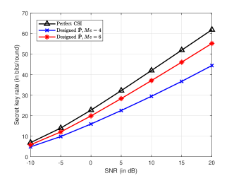
Figure 3: Secret key rate comparison for one UT.

First, we evaluate the performance of the beam domain secret key generation scheme in the single user scenario. Fig. 3 presents the secret key rate of single user, confirming that the proposed scheme can effectively reduce the dimension of the large channel matrix. The perfect CSI provides the complete channel information and achieves the highest secret key rate. We make a comparison between the secret key rate of the perfect CSI and that of our designed precoding matrices. Here, we consider $M_{e}=4$ and $M_{e}=6$ cases. The numerical results demonstrate that, when $M_{e}=6$, the secret key rate of designed matrices can approach the perfect case. This indicates that employing the precoding matrix ${\tilde{\mathbf{P}}}$ enables the BS and the UT to obtain the almost perfect channel information, while significantly reducing the pilot overhead and the dimension of channel estimation. When $M_{e}=4$, the secret key rate is a little smaller than that of $M_{e}=6$, which contains the most channel power with lower overhead.

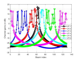
Figure 4: Multi-user channel gains distribution in the beam domain.

Next, we consider the multi-user secret key generation and illustrate an example of multi-user channel gains distribution in the beam domain in Fig. 4. The BS employs $128$ antennas to generate $128$ beams with different directions and the beam index $m$ represents the $m$th beam with direction $\sin(\varphi_{m})=2m/M-1$. When $6$ UTs are distributed in different positions, the channel gains of each UT are concentrated within a few beams, different UTs occupy non-overlapping channel beams. The attenuation between the adjacent UTs is about 20 dB, significantly reducing inter-user interference. This result indicates that the BS equipped with massive antennas has the potential to achieve multi-user secret key generation.

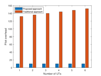
Figure 5: Pilot overhead for traditional and proposed approaches.

Fig. 5 compares the pilot overhead of traditional and proposed approaches multi-user secret key generation. We observe that due to the large number of antennas at the BS, the traditional overhead $T_{TA}$ is extremely large, meanwhile the overhead also scales with the number of UTs. In contract, the overhead of proposed approach with pilot reuse $T_{PA}$ remains the same and is significantly lower than that of the traditional approach. This result demonstrates the desirable performance of the proposed approach in reducing pilot overhead.

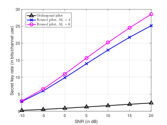
Figure 6: Secret key rate comparison for multiple UTs of orthogonal pilot and reused pilot.

Since the bottleneck is the pilot overhead in massive MIMO network, we must compare the secret key rate as well as the pilot overhead. Therefore, we define the unit secret key rate as $R_{\text{unit}}=R_{\text{sum}}/T$, where $T$ ($T_{TA}$ or $T_{PA}$) is the pilot overhead, scaled with the dimension of the effective channel $M_{e}$ and $N_{e}$. As the number of antennas at each UT is $4$, we set $N_{e}=N_{k}=4$. Fig. 6 compares the unit secret key rate of reused pilot with $M_{e}=4$ and $M_{e}=6$ with orthogonal pilot scheme. The unit secret key rate in orthogonal pilot schemes suffers serious loss due to its extremely large pilot overhead. The reused pilot scheme with $M_{e}=6$ achieves the highest rate and the scheme with $M_{e}=4$ is close to that of $M_{e}=6$.

VI Conclusion

This paper provided a design and analysis of the multi-user secret key generation in massive MIMO wireless communications. Exploiting the sparse property of the beam domain channel model, we proposed a channel dimension reduction algorithm named BCP to significantly reduce the dimension of the channel estimation. Furthermore, we presented a novel algorithm named IMBA which designs the precoding and receiving matrices to support multi-user key generation. Numerical results demonstrated the performance improvement of our proposed multi-user secret key generation scheme.

Appendix A Proof of Theorem 1

We assume zero-mean complex Gaussian random vector for each channel observation ${\mathbf{z}}_{k}^{DL}$ or ${\mathbf{z}}_{k}^{UL}$. When the channel observations of different UTs are uncorrelated, we have [9]

$$I_{k}=I({\mathbf{z}}_{k}^{DL};{\mathbf{z}}_{k}^{UL})=\log\frac{\det({\cal R}_{{\mathbf{z}}_{k}^{DL}}{\cal R}_{{\mathbf{z}}_{k}^{UL}})}{\det({\cal R}_{{\mathbf{z}}_{k}^{DL}{\mathbf{z}}_{k}^{UL}})},$$ (15)

which only depends on the correlation of uplink and downlink channels.

Let ${\mathbf{R}}_{k}={\mathbb{E}}\{{\rm{vec}}({\mathbf{H}}_{k}){\rm{vec}}({\mathbf{H}}_{k})^{H}\}$ be the full correlation of the channel matrix. We can calculate ${\cal R}_{{\mathbf{z}}_{k}^{DL}}$ as

$${\cal R}_{{\mathbf{z}}_{k}^{DL}}=\sum_{k^{\prime}}(({\mathbf{P}}_{k^{\prime}})^{T}\otimes{\mathbf{C}}_{k}^{H}){\mathbf{R}}_{k}\sum_{k^{\prime}}(({\mathbf{P}}_{k^{\prime}})^{T}\otimes{\mathbf{C}}_{k}^{H})^{H}$$

$$+({\mathbf{I}}_{T_{D}}\otimes{\mathbf{C}}_{k}^{H}{\mathbf{C}}_{k}).$$ (16)

Note that ${\mathbf{R}}_{k}$ can be decomposed as ${\mathbf{R}}_{k}=({\mathbf{A}}_{BS}^{*}\otimes{\mathbf{A}}_{UT})\hbox{\boldmath$\Lambda$}_{k}({\mathbf{A}}_{BS}^{*}\otimes{\mathbf{A}}_{UT})^{H}$. Let ${\tilde{\mathbf{P}}}_{k}={\mathbf{A}}_{BS}^{H}{\mathbf{P}}_{k}$, ${\tilde{\mathbf{C}}}_{k}={\mathbf{A}}_{UT,k}^{H}{\mathbf{C}}_{k}$, ${\mathbf{V}}_{k}=\hbox{\boldmath$\Lambda$}_{k}^{1/2}\Big{(}\sum_{k^{\prime}}({\tilde{\mathbf{P}}}_{k^{\prime}})^{T}\otimes{\tilde{\mathbf{C}}}_{k}^{H}\Big{)}^{H}$ and ${\mathbf{V}}_{kk^{\prime}}=\hbox{\boldmath$\Lambda$}_{k^{\prime}}^{1/2}\Big{(}{\tilde{\mathbf{P}}}^{T}_{k}\otimes{\tilde{\mathbf{C}}}^{H}_{k^{\prime}}\Big{)}^{H}$. The covariance matrix ${\cal R}_{{\mathbf{z}}_{k}^{DL}}$ can be rewritten as

$${\cal R}_{{\mathbf{z}}_{k}^{DL}}={\mathbf{V}}_{k}^{H}{\mathbf{V}}_{k}+({\mathbf{I}}_{T_{D}}\otimes{\mathbf{C}}_{k}^{H}{\mathbf{C}}_{k}).$$ (17)

Similarly, we can calculate ${\mathbf{R}}_{{\mathbf{z}}_{k}^{UL}}$ and ${\mathbf{R}}_{{\mathbf{z}}_{k}^{DL}{\mathbf{z}}_{k}^{UL}}$ as

$${\cal R}_{{\mathbf{z}}_{k}^{UL}}= \sum_{k^{\prime}}{\mathbf{V}}_{kk^{\prime}}^{H}{\mathbf{V}}_{kk^{\prime}}+({\mathbf{P}}^{T}_{k}{\mathbf{P}}^{*}_{k}\otimes{\mathbf{I}}_{T_{U}})$$

$${\mathbf{R}}_{{\mathbf{z}}_{k}^{DL}{\mathbf{z}}_{k}^{UL}}= {\mathbf{V}}_{k}^{H}{\mathbf{V}}_{kk}.$$ (18)

The covariance matrix ${\cal R}_{{\mathbf{z}}_{k}^{DL}{\mathbf{z}}^{UL}_{k}}$ can be decomposed as

$${\cal R}_{{\mathbf{z}}_{k}^{DL}{\mathbf{z}}^{UL}_{k}}=\begin{bmatrix}{\cal R}_{{\mathbf{z}}_{k}^{DL}}&{\mathbf{R}}_{{\mathbf{z}}_{k}^{DL}{\mathbf{z}}_{k}^{UL}}\\ {\mathbf{R}}_{{\mathbf{z}}_{k}^{UL}{\mathbf{z}}_{k}^{DL}}&{\cal R}_{{\mathbf{z}}_{k}^{UL}}.\end{bmatrix}$$ (19)

From the determinant of the block matrix, we have

$$\det({\cal R}_{{\mathbf{z}}_{k}^{DL}{\mathbf{z}}^{UL}_{k}})=\det({\cal R}_{{\mathbf{z}}_{k}^{DL}})\\ \times\det\Big{(}{\cal R}_{{\mathbf{z}}_{k}^{UL}}-{\mathbf{R}}_{{\mathbf{z}}_{k}^{UL}{\mathbf{z}}_{k}^{DL}}{\cal R}_{{\mathbf{z}}_{k}^{DL}}^{-1}{\mathbf{R}}_{{\mathbf{z}}_{k}^{DL}{\mathbf{z}}_{k}^{UL}}\Big{)}.$$ (20)

Then, the secret key rate can be expressed as

$$I_{k}=\!-\log\!\det\!\Bigg{(}\!{\mathbf{I}}-{\mathbf{V}}_{kk}\!\left(\!\sum_{k^{\prime}}{\mathbf{V}}_{kk^{\prime}}^{H}{\mathbf{V}}_{kk^{\prime}}\!+\!\Big{(}{\mathbf{P}}^{T}_{k}{\mathbf{P}}^{*}_{k}\otimes{\mathbf{I}}_{T_{U}}\!\Big{)}\!\!\right)^{-1}$$

$$\quad\times{\mathbf{V}}_{kk}^{H}{\mathbf{V}}_{k}\left({\mathbf{V}}_{k}^{H}{\mathbf{V}}_{k}+{\mathbf{I}}_{T_{D}}\otimes{\mathbf{C}}_{k}^{H}{\mathbf{C}}_{k}\right)^{-1}{\mathbf{V}}_{k}^{H}\Bigg{)}.$$ (21)

This completes the proof. ∎

References

• [1] G. Li, C. Sun, J. Zhang, E. Jorswieck, B. Xiao, and A. Hu, “Physical layer key generation in 5G and beyond wireless communications: Challenges and opportunities,” Entropy, vol. 21, no. 5, p. 497, 2019.
• [2] E. A. Jorswieck, A. Wolf, and S. Engelmann, “Secret key generation from reciprocal spatially correlated MIMO channels,” in Proc. IEEE Globecom Workshops, Atlanta, GA, USA, Jun. 2014, pp. 1–6.
• [3] L. Jiao, J. Tang, and K. Zeng, “Physical layer key generation using virtual AoA and AoD of mmwave massive MIMO channel,” in Proc. IEEE Conf. Communications and Network Security (CNS), May 2018, pp. 1–9.
• [4] J. Zhang, T. Q. Duong, A. Marshall, and R. Woods, “Key generation from wireless channels: A review,” IEEE Access, vol. 4, pp. 614–626, Mar. 2016.
• [5] J. Zhang, M. Ding, D. Lopez-Perez, A. Marshall, and L. Hanzo, “Design of an efficient ofdma-based multi-user key generation protocol,” IEEE Trans. Veh. Technol., vol. 68, no. 9, pp. 8842 – 8852, Sep. 2019.
• [6] D. Tse and P. Viswanath, Fundamentals of Wireless Communication.   New York, NY: Cambridge University Press, 2005.
• [7] C. Sun, X. Gao, S. Jin, M. Matthaiou, Z. Ding, and C. Xiao, “Beam division multiple access transmission for massive MIMO communications,” IEEE Trans. Commun., vol. 63, no. 6, pp. 2170–2184, Jun. 2015.
• [8] O. E. Ayach, S. Rajagopal, S. Abu-Surra, Z. Pi, and R. W. Heath, “Spatially sparse precoding in millimeter wave MIMO systems,” IEEE Trans. Wireless Commun., vol. 13, no. 3, pp. 1499–1513, March 2014.
• [9] J. W. Wallace and R. K. Sharma, “Automatic secret keys from reciprocal MIMO wireless channels: Measurement and analysis,” IEEE Trans. Inf. Forensics Security, vol. 5, no. 3, pp. 381–392, Sep. 2010.