Deep Convolutional Sparse Coding Networks for Image Fusion

Abstract

Image fusion is a significant problem in many fields including digital photography, computational imaging and remote sensing, to name but a few. Recently, deep learning has emerged as an important tool for image fusion. This paper presents three deep convolutional sparse coding (CSC) networks for three kinds of image fusion tasks (i.e., infrared and visible image fusion, multi-exposure image fusion, and multi-modal image fusion). The CSC model and the iterative shrinkage and thresholding algorithm are generalized into dictionary convolution units. As a result, all hyper-parameters are learned from data. Our extensive experiments and comprehensive comparisons reveal the superiority of the proposed networks with regard to quantitative evaluation and visual inspection.

I Introduction

Image fusion is a fundamental topic in image processing [6], and its aim is to generate a fusion image by combining the complementary information of source images [21]. This technique has been applied to many scenarios. For example, in military, infrared and visible image fusion (IVF) is helpful for object detection and recognition [24]. In digital photography, high dynamic range (HDR) imaging can be solved by multi-exposure image fusion (MEF) to generate high-contrast and informative images [26].

Over the past a few decades, numerous image fusion algorithms have been proposed, where transform based algorithms are very popular [21]. They transform source images into feature domain, detect the active levels, blend the features and at last apply the inverse transformer in order to obtain the fused image. Recently, deep neural networks have emerged as an effective tool in image fusion [21]. They are divided into three groups: (1) Autoencoder based methods. This is a deep learning variant of transform based algorithms. The transformers and inverse transformers are replaced by encoders and decoders, respectively [16]. (2) Supervised methods. For multi-focus image fusion, there are ground truth images in the synthetic datasets [20]. For MEF, Cai et al. constructed a large dataset providing the reference images by comparing 13 MEF/HDR algorithms [4]. Owing to the strong fitting ability, supervised learning networks are suitable for these tasks. (3) Human visual system based methods. In the case without reference image, by taking prior knowledge into account and setting proper loss functions, researchers designed regression [44, 27] or adversarial [25] networks to make fusion images satisfy human visual systems. However, it is found that many algorithms are evaluated on a limited number of cherry-picked images. Thus, their generalizations still remain unknown. It leaves room for possible improvement with reasonable and interpretable formulations.

Convolutional sparse coding (CSC) has been successfully applied to computer vision tasks on account of its high performance and robustness [40, 12]. The CSC model is generally solved by the iterative shrinkage and thresholding algorithm (ISTA), but the results significantly depend on hyper-parameters. To address this problem, the CSC model and ISTA are generalized into some dictionary convolutional units (DCUs) which are put in the hidden layers of neural networks. In this manner, the hyper-parameters (e.g. penalty parameters, dictionary filters and thresholding functions) in DCUs are learnable. Based on the novel unit, we design deep CSC networks for three fusion tasks, including IVF, MEF, and multi-modal image fusion (MMF). In our experiments, we employ relatively large test datasets to make a comprehensive and convincing evaluation. Experimental results show that the deep CSC networks outperform the state-of-the-art (SOTA) methods in terms of both objective metrics and visual inspection. Besides, our networks are with high reproducibility. The remainder of this paper is organized as follows. Section II converts the CSC and ISTA into a DCU. Then, in section III we design three DCU based networks for IVF, MEF and MRF tasks. The extensive experiments are reported in section IV. Section V concludes this paper.

II Dictionary Convolutional Units

In dictionary learning, CSC is a typical method for image processing. Given an image $\bm{x}\in R^{c\times h\times w}$ ($c=1$ for gray images and $c=3$ for RGB images) and $q$ convolutional filters $\bm{d}\in R^{q\times c\times s\times s}$, CSC can be formulated as the following problem:

$$\min_{\bm{z}}\frac{1}{2}\|\bm{x}-\bm{d}*\bm{z}\|_{2}^{2}+\lambda g(\bm{z}),$$ (1)

where $\lambda$ is a hyperparameter, $*$ denotes the convolution operator, $\bm{z}\in R^{q\times h\times w}$ is the sparse feature map (or say, code) and $g(\cdot)$ is a sparse regularizer. This problem can be solved by ISTA, and it is easy to write the updating rule for feature maps as below,

$$\bm{z}^{(k+1)}\leftarrow\mathrm{prox}_{\lambda/\rho}\left(\bm{z}^{(k)}+\frac{1}{\rho}\bm{d}^{T}*(\bm{x}-\bm{d}*\bm{z}^{(k)})\right),$$ (2)

where $\rho$ is the step size and $\bm{d}^{T}\in R^{c\times q\times s\times s}$ is the flipped version of $\bm{d}$ along horizontal and vertical directions. Note that $\mathrm{prox}(\cdot)$ is the proximal operator of the regularizer $g(\cdot)$. If $g(\cdot)$ is the $\ell_{1}$-norm, its corresponding proximal operator is the soft shrinkage thresholding (SST) function defined by $\mathrm{SST}_{\gamma}(x)=\mathrm{sign}(x)\mathrm{ReLU}(|x|-\gamma),$ where $\mathrm{ReLU}(x)=\max(x,0)$ is the rectified linear unit and $\mathrm{sign}(x)$ is the sign function. CSC provides a pipeline to extract features of an image, but its performance highly depends on the configuration of $\{\lambda,\rho,\bm{d}\}$. By the principle of algorithm unrolling [33, 39, 9], the ISTA of CSC can be generalized as a unit in neural networks. We employ two convolutional units, $\mathrm{Conv}_{i}(i=0,1)$, to replace $\bm{d}$ and $\bm{d}^{T}/\rho$, and proximal operator $\mathrm{prox}(\cdot)$ is extended to the activation function $f(\cdot)$. Hence, Eq.(2) can be rewritten as

$$\bm{z}^{(k+1)}=f\left({\rm BN}\left(\bm{z}^{(k)}+\mathrm{Conv}_{1}(\bm{x}-\mathrm{Conv}_{0}(\bm{z}^{(k)}))\right)\right),$$ (3)

where we also take batch normalization (BN) into account. It is worth pointing out that, except for SST, the activation function can be freely set to alternatives (e.g., ReLU, parametric ReLU (PReLU) and so on) if the regularizer $g(\cdot)$ is not set to $\ell_{1}$-norm. In what follows, Eq. (3) is called a dictionary convolutional unit (DCU). By stacking DCUs, the original CSC model can be represented as a deep CSC neural network.

In addition, stacking DCUs is interpretable to representation learning. $\mathrm{Conv}_{0}$ serves as a decoder, since it maps $\bm{z}^{(k)}$ from feature space to image space. And $\mathrm{Conv}_{1}$ serves as an encoder, since it maps the residual between the original image $\bm{x}$ and the reconstructed image $\mathrm{Conv}_{0}(\bm{z}^{(k)})$ from image space to feature space. Then, the encoded residual is added to the current code $\bm{z}^{(k)}$ for updating. Eventually, the output passes through BN and an activation function for non-linearity. This process can be regarded as an iterative auto-encoder.

III Deep Convolutional Sparse Coding Based Image Fusion

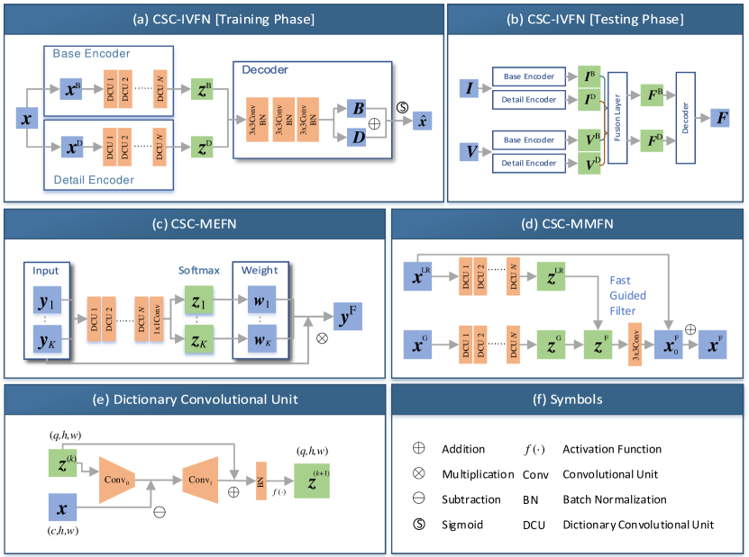
Figure 1: Network structure.

In this section, we apply deep CSC neural networks to the image fusion problem, and exhibit three paradigms of model formulation for three different image fusion tasks.

III-A Infrared and Visible Image Fusion

By combining autoencoders and the CSC model, we propose a CSC-based IVF network (CSC-IVFN), which can be regarded as a flexible data-driven transformer. In the training phase, we train CSC-IVFN in the autoencoder fashion. In the testing phase, features obtained by the encoder of CSC-IVFN are fused and the fusion image is decoded by a decoder.

III-A1 Training Phase

The architecture is displayed in Fig. 1 (a). Firstly, the input image $\bm{x}$ is decomposed into a base image $\bm{x}^{\rm B}$ containing low-frequency information and a detail image $\bm{x}^{\rm D}$ containing high-frequency textures. Similar to [22, 14], $\bm{x}^{\rm B}$ is obtained by applying a box-blur filter to $\bm{x}$, and as for the detail image there is $\bm{x}^{\rm D}=\bm{x}-\bm{x}^{\rm B}$. Then, the base and detail images pass through $N$ stacked DCUs, and we will get the final feature maps, that is, $\bm{z}^{\rm D}$ and $\bm{z}^{\rm B}$. And next we feed them into a decoder to decode the base and detail images. Finally, they are combined to reconstruct the input image. Here, the output is activated by a sigmoid function to make sure that the values range from 0 to 1. The loss function is mean squared error (MSE) plus structural similarity (SSIM) loss,

$$L^{\rm IVF}=\frac{1}{hw}\left(\|\bm{x}-\hat{\bm{x}}\|_{2}^{2}+\lambda^{\rm IVF}\frac{1-{\rm SSIM}(\bm{x},\hat{\bm{x}})}{2}\right),$$ (4)

where $\lambda^{\rm IVF}$ is a trade-off parameter to balance the MSE and SSIM [42]. Note that MSE is used to keep the spatial consistency and SSIM guarantees local details in terms of structure, contrast and brightness [42].

III-A2 Testing Phase

After training a CSC-IVFN, there is a transformer (encoder) and inverse transformer (decoder). In the test phase, CSC-IVFN is feed with a pair of infrared and visible images. In what follows, we use $\bm{I}^{\rm B}$, $\bm{I}^{\rm D}$, $\bm{V}^{\rm B}$ and $\bm{V}^{\rm D}$ to represent the base and detail feature maps of infrared and visible images, respectively. As exhibited in Fig. 1 (b), a fusion layer is inserted between encoder and decoder in the test phase. It can be expressed by a unified merging operation $\mathcal{F}(\cdot)$,

$$\bm{F}^{\rm B}=\mathcal{F}(\bm{I}^{\rm B},\bm{V}^{\rm B})=\bm{w}_{1}^{\rm B}\otimes\bm{I}^{\rm B}\oplus\bm{w}_{2}^{\rm B}\otimes\bm{V}^{\rm B},$$ (5)

$$\bm{F}^{\rm D}=\mathcal{F}(\bm{I}^{\rm D},\bm{V}^{\rm D})=\bm{w}_{1}^{\rm D}\otimes\bm{I}^{\rm D}\oplus\bm{w}_{2}^{\rm D}\otimes\bm{V}^{\rm D}.$$

Here, $\otimes$ and $\oplus$ are element-wise product and addition. There are three popular fusion strategies:

1. Average strategy: $\displaystyle{\bm{w}_{1}^{\rm B}=\bm{w}_{1}^{\rm D}=\bm{w}_{2}^{\rm B}=\bm{w}_{2}^{\rm D}=0.5}$.

2. IVF $\ell_{1}$-norm fusion strategy[16, 22]: It uses the $\ell_{1}$-norm of patches as the active level. For base weights, there are

   $$\bm{w}_{1}^{\rm B} ={\Gamma\left({{{\left\|\bm{I}^{\rm B}\right\|}_{1}}}\right)}/\left[{\Gamma\left({{{\left\|\bm{I}^{\rm B}\right\|}_{1}}}\right)+\Gamma\left({{{\left\|\bm{V}^{\rm B}\right\|}_{1}}}\right)}\right],$$ (6)

   $$\bm{w}_{2}^{\rm B} =1-\bm{w}_{1}^{\rm B},$$

   where $\Gamma(\cdot)$ is a $3\times 3$ mean filter. The detail weights $\bm{w}_{1}^{\rm D}$ and $\bm{w}_{2}^{\rm D}$ can be obtained in the same way.

3. Saliency-weighted fusion strategy [14]: To highlight and retain the saliency target and information, the fusion weight of this strategy is determined by the saliency degree. We take base weights as an example. Firstly, the saliency value of $\bm{I}^{\rm B}$ at the $k$th pixel can be obtained by $\bm{S}_{\bm{I}}^{\rm B}(k)=\sum_{i=0}^{255}\bm{H}^{\rm B}_{\bm{I}}(i)|\bm{I}^{\rm B}(k)-i|,$ where $\bm{I}^{\rm B}(k)$ is the value of the $k$th pixel and $\bm{H}^{\rm B}_{\bm{I}}(i)$ is the frequency of pixel value $i$. The initial weight at the $k$th pixel is $\tilde{\bm{w}}_{1}^{\rm B}(k)={\bm{S}_{\bm{I}}^{\rm B}(k)}/\left[{\bm{S}_{\bm{I}}^{\rm B}(k)+\bm{S}_{\bm{V}}^{\rm B}(k)}\right]$ and $\tilde{\bm{w}}_{2}^{\rm B}(k)=1-\tilde{\bm{w}}_{2}^{\rm B}(k)$. To prevent region boundaries and artifacts, the weight map is refined via the guided filter $\mathcal{G}(\cdot,\cdot)$ with the guidance of base and detail feature maps:

   $$\bm{w}_{1}^{\rm B} =\mathcal{G}({\tilde{\bm{w}}_{1}^{\rm B}},\bm{I}^{\rm B})/\left[\mathcal{G}({\tilde{\bm{w}}_{1}^{\rm B}},\bm{I}^{\rm B})+\mathcal{G}({\tilde{\bm{w}}_{2}^{\rm B}},\bm{I}^{\rm V})\right],$$ (7)

   $$\bm{w}_{2}^{\rm B} =1-\bm{w}_{1}^{\rm B}.$$

III-B Multi-Exposure Image Fusion

Most of MEF algorithms fall under the umbrella of weighted summation framework, $\bm{f}=\sum_{k=1}^{K}\bm{w}_{k}\otimes\bm{x}_{k},$ where $\{\bm{x}_{k}\}_{k=1}^{K}$ are source images, $\{\bm{w}_{k}\}_{k=1}^{K}$ are the corresponding weight maps, $\bm{f}$ is the fused image and $K$ denotes the number of exposures. We propose a CSC-based MEF network (CSC-MEFN). Different from CSC-IVFN, CSC-MEFN is an end-to-end network. Here DCUs extract feature maps, which are then used to predict weight maps to generate the fusion image. To avoid chroma distortion, the proposed CSC-MEFN works in the YCbCr space, and its channels are denoted by $\bm{y}_{k},\bm{b}_{k}$ and $\bm{r}_{k}$. As shown in Fig. 1 (c), Y channels $\{\bm{y}_{k}\}_{k=1}^{K}$ pass through CSC-MEFN one-by-one. At first, CSC-MEFN stacks $N$ DCUs to code the Y channels. Then, it is followed by a $1\times 1$ convolutional unit to get the final code $\bm{z}_{k}$. Thereafter, the codes $\{\bm{z}_{k}\}_{k=1}^{K}$ are converted into weight maps $\{\bm{w}_{k}\}_{k=1}^{K}$ by softmax activation. At last, the fused Y channel $\bm{y}^{\rm F}$ is obtained by $\bm{y}^{\rm F}=\sum_{k=1}^{K}\bm{w}_{k}\otimes\bm{y}_{k}$. As for the Cb channels, we employ the MEF $\ell_{1}$-norm fusion strategy, i.e., $\bm{b}^{\rm F}=\sum_{k=1}^{K}\|\bm{b}_{k}-0.5\|_{1}\bm{b}_{k}/\sum_{k=1}^{K}\|\bm{b}_{k}-0.5\|_{1}.$ So Cr channels do. After the separate fusion of three channels, the fusion image $\bm{f}$ is transformed from YCbCr to RGB space. Eventually, we apply a post-processing [19]: the values at 0.5% and 99.5% intensity level are mapped to [0,1], and values out of this range are clipped.

CSC-MEFN is supervised by improved MEFSSIM [26]. It evaluates the similarity between source images $\{\bm{x}_{k}\}_{k=1}^{K}$ and the fusion image $\bm{f}$ in terms of illumination, contrast and structure. Our experimental results show that MEFSSIM often leads to haloes. Essentially, halo artifacts result from the pixel fluctuation in the illumination map (i.e., Y channel). To suppress haloes, we propose a halo loss defined by the $\ell_{1}$-norm on gradients of the illumination map, $L_{\rm halo}=\|\nabla\bm{y}^{\rm F}\|_{1},$ where $\nabla$ denotes the image gradient operator (see details in supplementary materials). In our experiments, $\nabla$ is implemented by horizontal and vertical Sobel filters. In summary, given the penalty parameter $\lambda^{\rm MEF}$, the loss function of CSC-MEFN is expressed by

$$L^{\rm MEF}=\frac{1}{hw}\left(-{\rm MEFSSIM}+\lambda^{\rm MEF}L_{\rm halo}\right).$$ (8)

III-C Multi-Modal Image Fusion

Owing to the limitation of multispectral imaging devices, multispectral images (MS) contain enriched spectral information but with low resolution (LR). One of the promising techniques for acquiring a high resolution (HR) MS is to fuse the LRMS with a guidance image (e.g. panchromatic or RGB images). This problem is a special MMF task. We present a CSC-based MMF network (CSC-MMFN) for the general MMF task. It is assumed that LR and guidance images are represented by $\bm{x}^{\rm LR}=\bm{d}^{\rm LR}*\bm{z}^{\rm LR}$ and $\bm{x}^{\rm G}=\bm{d}^{\rm G}*\bm{z}^{\rm G},$ respectively. Given the dictionary of HR images $\bm{d}^{\rm F}$, the HR image is represented by

$$\bm{x}^{\rm F}=\bm{d}^{\rm F}*(\bm{z}^{\rm LR})\uparrow.$$ (9)

The symbol $\uparrow$ denotes the upsampling operator. According to this model, CSC-MMFN separately extracts codes of $\bm{x}^{\rm LR}$ and $\bm{x}^{\rm G}$ by two sequences of DCUs, and we utilize the fast guidance filter to super-resolve $\bm{z}^{\rm LR}$ with the guidance of $\bm{z}^{\rm G}$. At last, the HR image is recovered by a $3\times 3$ convolutional unit. The loss function is set to MSE between ground-truth and fusion images.

IV Experiments

TABLE I: Datasets employed in this paper.

IVF	Training		Validation			Test
	FLIR-Train		NIR-Water	NIR-OldBuilding		TNO	FLIR-Test	NIR-Country
# Pairs	180		51	51		40	40	52
Illumination	Day&Night		Day	Day		Night	Day&Night	Day
Objectives	Individual&Stuff		Scenery	Building		Individual&Stuff	Individual&Stuff	Scenery

MEF	Training		Validation			Test
	SICE-Train		SICE-Val	TCI2018		HDRPS
# Pairs	466		51	24		44
# Exposures	6-28		5-20	3-30		9

MMF	Cave
# Train/Validation/Test	22/4/6
LR Image	Multispectral
Guide Image	RGB

Here we elaborate the implementation and configuration details of our networks. Experiments are conducted to show the performance of our models and the rationality of network structures. For each task, our experiments utilized training, validation and test datasets. The hyperparameters are determined by validation set.

IV-A Infrared and Visible Image Fusion

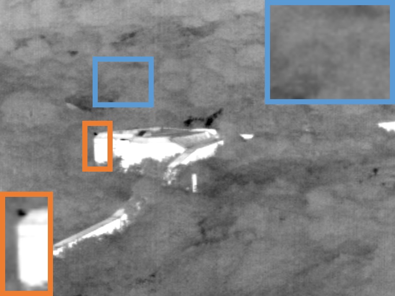
(a) Infrared

(b) Visible

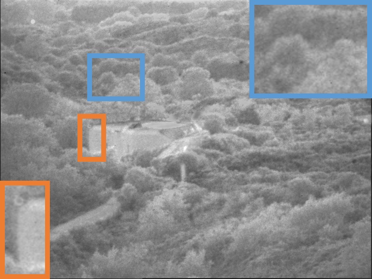
(c) ADKT

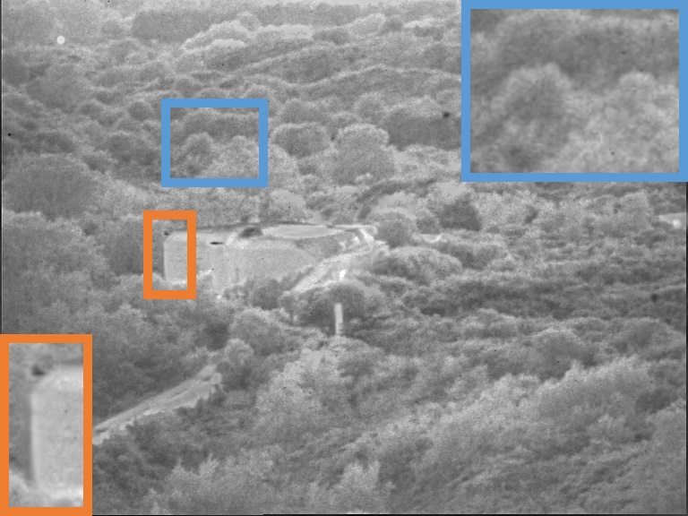
(d) CSR

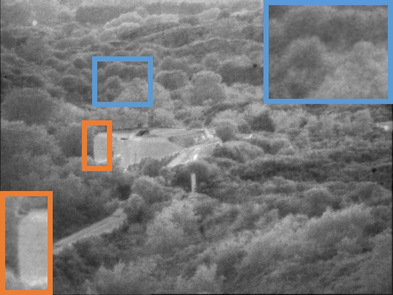
(e) DeepFuse

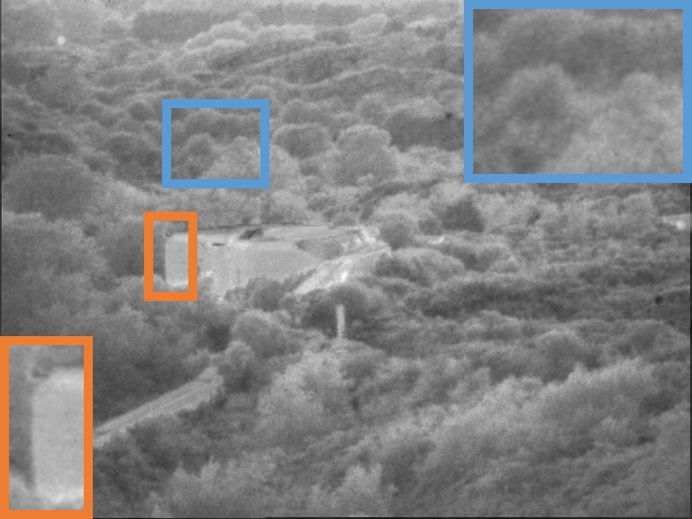
(f) DenseFuse

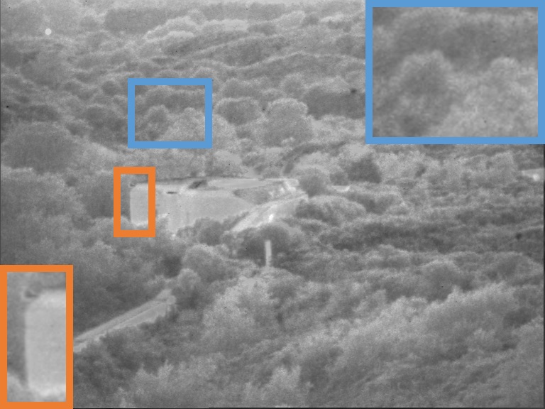
(g) DLF

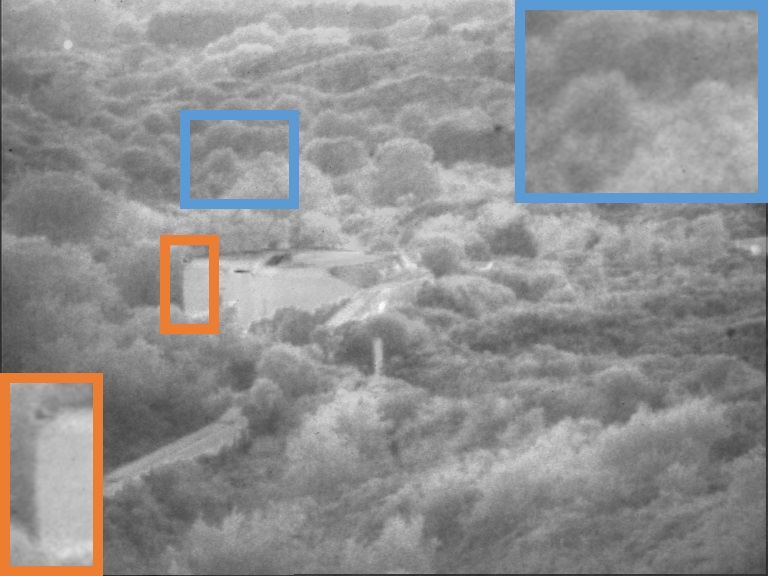
(h) FEZL

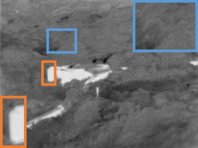
(i) FusionGan

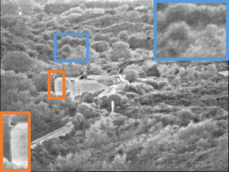
(j) SDF

(k) TVAL

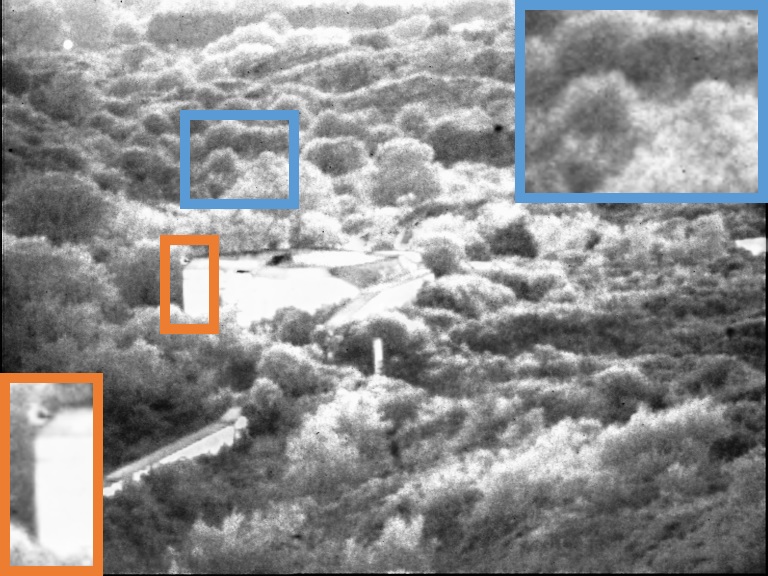
(l) Ours

Figure 2: The fused images of Bunker.

IV-A1 Datasets, Metrics and Details

As shown in Table I, IVF experiments use three datasets (FLIR, NIR and TNO). The 180 pairs of images in FLIR compose the training set. Two subsets (Water and OldBuilding) of NIR are used for validation. To comprehensively evaluate the performance of different models, we employ TNO, NIR-Country and the rest pairs of FLIR as test datasets. To the best of our knowledge, most of the papers only employ part of cherry-picked pairs in TNO as test sets. However, our test sets contain more than 130 pairs with different illuminations and scenarios. To quantitatively measure the fusion performance, six metrics are employed: entropy (EN) [37], standard deviation (SD) [36], spatial frequency (SF) [8], visual information fidelity (VIF) [11], average gradient (AG) [5] and sum of the correlations of differences (SCD) [1]. Larger metrics indicate that a fusion image is better. In our experiment, the tuning parameter $\lambda^{\rm IVF}$ in Eq. (4) is set to 5. The network is optimized over 60 epochs with a learning rate of $10^{-2}$ in the first 30 epochs and $10^{-3}$ in the rest epochs. The number of DCUs, activation function and fusion strategy may significantly affect the performance of CSC-IVFN. We determine them on validation sets. With the limited space, the validation experiments are exhibited in supplementary materials and the best configuration is reported as follows: the number of DCUs in base or detail encoder is 7; the activation functions in base and detail encoders are set as PReLU and SST, respectively; the fusion strategies for base and detail images are saliency-weighted fusion and IVF $\ell_{1}$-norm fusion, respectively.

IV-A2 Comparison with SOTA Methods

To verify the superiority of our CSC-IVFN, we compare its fusion results with nine popular IVIF fusion methods, including ADKT [2], CSR [22], DeepFuse [35], DenseFuse [16], DLF [17], FEZL [14], FusionGAN [25], SDF [3] and TVAL [10]. Six metrics of all methods are displayed in Table II. It is shown that our method achieves the best performance on all test sets with regard to most metrics. Therefore, our method is suitable for various scenarios with different kinds of illuminations and object categories. In contrast, the other methods (including DeepFuse, DenseFuse and SDF) can achieve good performance on certain test sets with regard to a part of metrics. Besides the metric comparison, representative fusion images are displayed in Fig. 2. In the visible image, there are lots of bushes. In the infrared image, we can observe a bunker. However, it is not easy to recognize the bushes/bunker in the infrared/visible image. It is found that our fusion image keeps the details and textures of the visible image, and preserves the interest objects (i.e., the bushes and the bunker). In addition, its contrast is fairly high. In conclusion, both visible spectrum and thermal radiation information are retained in our fusion image. However, other methods cannot generate satisfactory images as good as ours.

TABLE II: Quantitative results of the IVF task. Boldface and underline indicate the best and the second best results, respectively.

Dataset: FLIR
	ADKT	CSR	DeepFuse	DenseFuse	DLF	FEZL	FusianGAN	SDF	TVAL	Ours
EN	6.80	6.91	7.21	7.21	6.99	6.91	7.02	7.15	6.80	7.61
MI	2.72	2.57	2.73	2.73	2.78	2.78	2.68	2.31	2.47	3.02
SD	28.37	30.53	37.35	37.32	32.58	31.16	34.38	35.89	28.07	55.94
SF	14.48	17.13	15.47	15.50	14.52	14.16	11.51	18.79	14.04	21.85
VIF	0.34	0.37	0.50	0.50	0.42	0.33	0.29	0.50	0.33	0.70
AG	3.56	4.80	4.80	4.82	4.15	3.38	3.20	5.57	3.52	6.92
SCD	1.39	1.42	1.72	1.72	1.57	1.42	1.18	1.50	1.40	1.80
Dataset: NIR-Country Scene
	ADKT	CSR	DeepFuse	DenseFuse	DLF	FEZL	FusianGAN	SDF	TVAL	Ours
EN	7.11	7.17	7.30	7.30	7.22	7.19	7.06	7.30	7.13	7.36
MI	3.94	3.70	4.04	4.04	3.97	3.81	3.00	3.29	3.67	3.86
SD	38.98	40.38	45.82	45.85	42.31	44.44	34.91	43.74	40.47	69.37
SF	17.31	20.37	18.63	18.72	18.36	17.04	14.31	20.65	16.69	28.29
VIF	0.54	0.58	0.68	0.68	0.61	0.55	0.42	0.69	0.53	1.05
AG	5.38	6.49	6.18	6.23	5.92	5.38	4.56	6.82	5.32	9.42
SCD	1.09	1.12	1.37	1.37	1.22	1.14	0.51	1.19	1.09	1.73
Dataset: TNO
	ADKT	CSR	DeepFuse	DenseFuse	DLF	FEZL	FusianGAN	SDF	TVAL	Ours
EN	6.40	6.43	6.86	6.84	6.38	6.63	6.58	6.67	6.40	6.91
MI	2.01	1.99	2.30	2.30	2.15	2.23	2.34	1.72	2.04	2.50
SD	22.96	23.60	32.25	31.82	22.94	28.05	29.04	28.04	23.01	46.97
SF	10.78	11.44	11.13	11.09	9.80	9.46	8.76	12.60	9.03	12.88
VIF	0.29	0.31	0.58	0.57	0.31	0.31	0.26	0.46	0.28	0.62
AG	2.99	3.37	3.60	3.60	2.72	2.55	2.42	3.98	2.52	4.22
SCD	1.61	1.63	1.80	1.80	1.62	1.67	1.40	1.68	1.60	1.70

IV-B Multi-Exposure Image Fusion

IV-B1 Datasets, Metrics and Details

Three datasets SICE [4], TCI2018 [26] and HDRPS are employed in our experiments. HDRPS and TCI2018 are used for test and validation, respectively. SICE is a large and high-quality dataset. It is divided into two parts for training and validation. The basic information of datasets is shown in Table I. Many papers use MEFSSIM to evaluate the performance, but CSC-MEFN is supervised by MEFSSIM. Hence, it is unfair for other methods. As an alternative, we utilize four SOTA blind image quality indices , i.e., blind/referenceless image spatial quality evaluator (Brisque) [31], naturalness image quality evaluator (Niqe) [32], perception based image quality evaluator (Piqe) [34] and multi-task end-to-end optimized deep neural network (MEON) based blind image quality assessment [28]. Smaller values indicate that a fusion image is better. Experiments show that large $\lambda^{\rm MEF}$ makes training unstable, so at the $i$th iteration it is set to $\min\{0.25(i-1),\lambda^{\rm MEF}_{\max}\}$. We select $\lambda^{\rm MEF}_{\max}=10$ to make halo loss and MEFSSIM loss have similar magnitudes. The network is optimized by Adam over 50 epochs with a learning rate of $5\times 10^{-4}$. The network configuration is determined by validation datasets. We utilize $N=3$ DCUs to extract codes and SST is employed as an activation function.

IV-B2 Comparison with SOTA Methods

CSC-MEFN is compared with seven classic and recent SOTA methods, including EF [30], GGIF [13], DenseFuse [16], MEF-Net [27], FMMR [18], DSIFTEF [23], Lee18 [15]. The metrics are listed in Table III. Our network outperforms other methods. Lee18 and EF are ranked in the second and third places. Fig. 3 displays the fusion images. It is shown that GGIF, MEF-Net, FMMR, DSIFTEF and Lee18 suffer from strongly halo effects around edges between the sky and rocks. For EF the right rock is too dark, and for DenseFuse the sun cannot be recognized. The contrast of local regions for both EF and DenseFuse is low. Our fusion image strikes the balance.

TABLE III: Quantitative results of the MEF task. Boldface and underline indicate the best and the second best results, respectively.

	EF	GGIF	DenseFuse	MEF-Net	FMMR	DSIFTEF	Lee18	Ours
MEON	8.6730	9.1537	11.8453	9.3623	9.8616	9.3787	9.8093	8.1776
Brisque	18.8259	19.1711	26.4427	19.4511	20.1099	18.6533	18.5110	18.2694
Niqe	2.9086	2.5204	2.5772	2.5215	2.5494	2.5277	2.4655	2.3980
Piqe	31.0617	32.1874	29.6126	32.2904	32.0856	32.2915	32.5380	27.8342

(a) EF

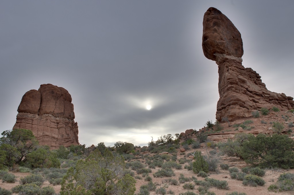
(b) GGIF

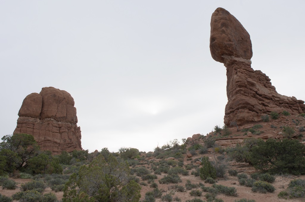
(c) DenseFuse

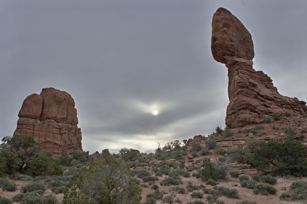
(d) MEF-Net

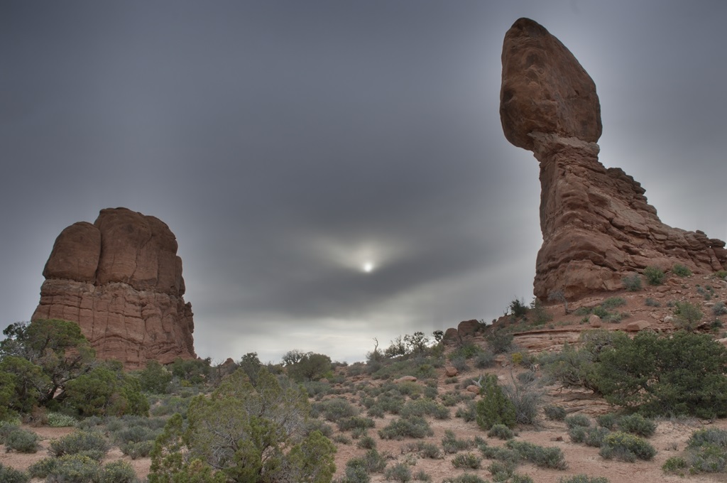
(e) FMMR

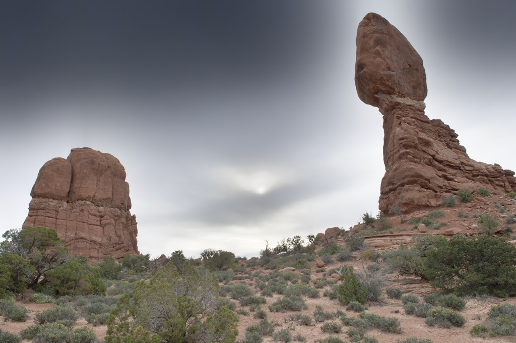
(f) DSIFTEF

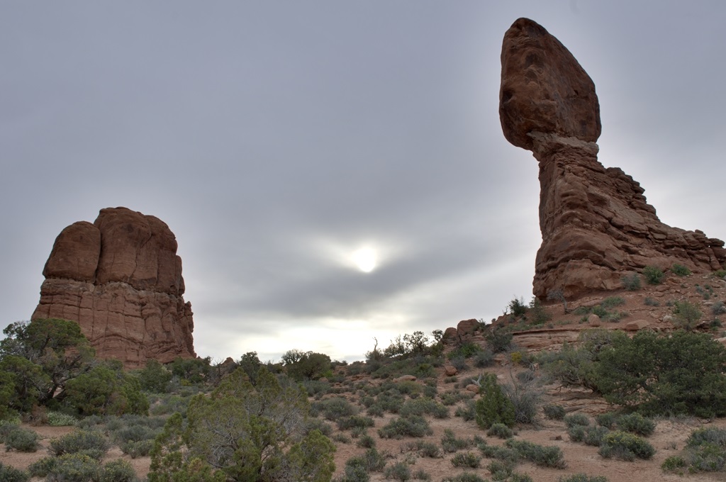
(g) Lee18

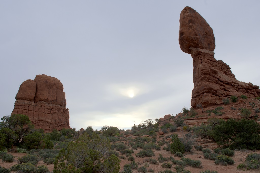
(h) Ours

Figure 3: The fused images of Balanced Rock.

IV-C Multi-Modal Image Fusion

IV-C1 Datasets, Metrics and Details

As shown in Table I, we employ a multispectral/RGB image fusion dataset, Cave [45]. It contains 32 scenes, each of which has a 31-band multispectral image and an RGB image. It is divided into three parts for training, testing and validation. The Wald protocol is used to construct training sets. We employ peak signal-to-noise ratio (PSNR) and SSIM as evaluation indexes. Larger PSNR and SSIM indicate that a fusion image is better. The network is optimized by Adam over 100 epochs with a learning rate of $5\times 10^{-4}$. SST is employed as an activation function. The number of DCUs is empirically set to 4 for a speed and accuracy trade-off.

IV-C2 Comparison with SOTA Methods

CSC-MMFN is compared with seven classic and recent SOTA methods, including CNMF [46], GSA [41], FUSE [43], MAPSMM [7], GLPHS [38], PNN [29] and PFCN [47]. The metrics listed in Table IV show that our network achieves the largest PSNR and SSIM. GLPHS and PFCN can be ranked in the second place in terms of PSNR and SSIM, respectively. The error maps of the third band of stuffed toys are displayed in Fig. 4. We found that CNMF, GSA and PFCN break down when reconstructing the color checkerboard and stuffed toys, while FUSE, MAPSMM, GLPHS and PNN perform badly at the edges. In summary, CSC-MMFN has the best performance.

TABLE IV: Quantitative results of the MMF task. Boldface and underline indicate the best and the second best results, respectively.

Images	CNMF			GSA			FUSE			MAPSMM
	PSNR	SSIM		PSNR	SSIM		PSNR	SSIM		PSNR	SSIM
R&F apples	34.5743	0.9384		32.7312	0.6816		38.2509	0.9434		41.4403	0.9786
R&F peppers	33.1338	0.9305		30.9636	0.7026		35.7674	0.9177		39.5621	0.9670
Sponges	31.1378	0.9549		26.3144	0.7429		33.7565	0.9368		35.2542	0.9347
Stuffed toys	30.0417	0.8652		27.3283	0.5764		34.3008	0.9372		36.4635	0.9449
Superballs	21.2880	0.8292		32.5318	0.7626		36.3646	0.9078		27.5589	0.6020
Thread spools	32.3698	0.8921		30.6611	0.6591		33.9568	0.9088		34.9208	0.9397
Mean	30.4242	0.9017		30.0884	0.6875		35.3995	0.9253		35.8666	0.8945
Images	GLPHS			PNN			PFCN			Ours
	PSNR	SSIM		PSNR	SSIM		PSNR	SSIM		PSNR	SSIM
R&F apples	43.5554	0.9873		39.9322	0.9681		41.5981	0.9864		51.5897	0.9954
R&F peppers	41.6063	0.9822		39.4820	0.9666		40.4695	0.9835		49.5495	0.9947
Sponges	37.2994	0.9735		31.3927	0.9573		32.0306	0.9830		43.2901	0.9873
Stuffed toys	38.3917	0.9756		33.6743	0.9585		33.1012	0.9713		44.1118	0.9897
Superballs	39.3176	0.9494		36.9901	0.9533		36.7382	0.9756		46.2919	0.9873
Thread spools	36.3586	0.9558		35.8109	0.9540		38.8272	0.9863		42.5585	0.9857
Mean	39.4215	0.9706		36.2137	0.9596		37.1275	0.9810		46.2319	0.9900

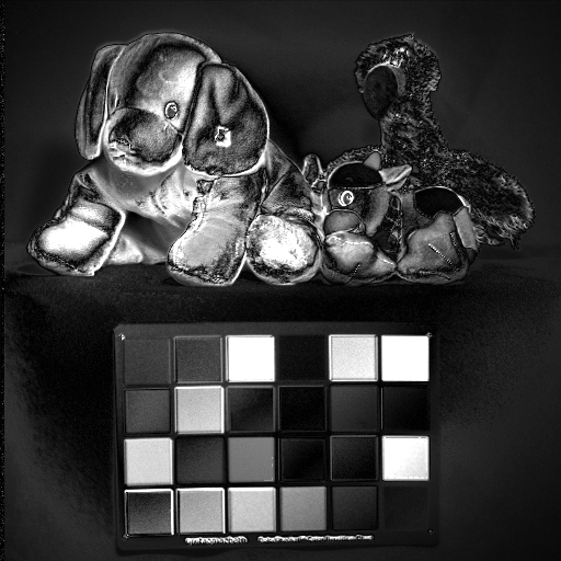
(a) CNMF

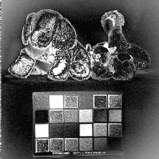
(b) GSA

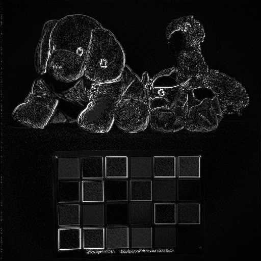
(c) FUSE

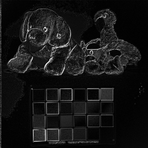
(d) MAPSMM

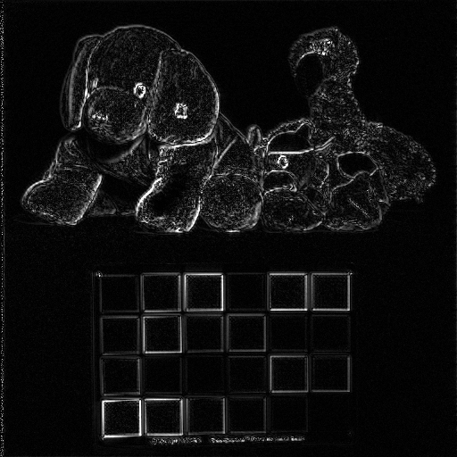
(e) GLPHS

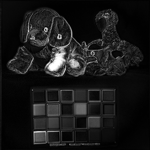
(f) PNN

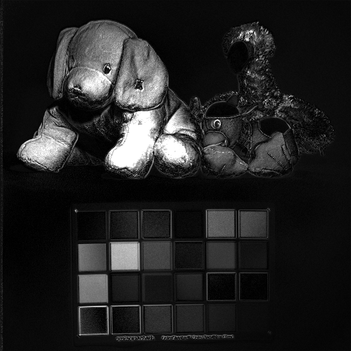
(g) PFCN

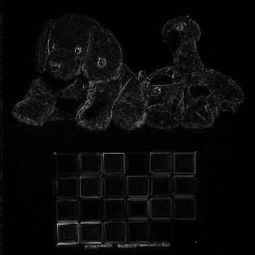
(h) Ours

Figure 4: The error maps of stuffed toys (band 3). Their values are amplified 10 times for easier visual inspection. The error goes larger from black to white.

V Conclusion

Inspired by converting the ISTA and CSC models into a hidden layer of neural networks, this paper proposes three deep CSC networks for IVF, MEF and MMF tasks. Extensive experiments and comprehensive comparisons demonstrate that our networks outperform the SOTA methods. Furthermore, the experiments in supplementary materials show that our networks are highly reproducible.

References

- [1] V Aslantas and E Bendes. A new image quality metric for image fusion: the sum of the correlations of differences. AEU - International Journal of Electronics and Communications, 69(12):1890–1896, 2015.
- [2] Durga Prasad Bavirisetti and Ravindra Dhuli. Fusion of infrared and visible sensor images based on anisotropic diffusion and karhunen-loeve transform. IEEE Sensors Journal, 16(1):203–209, 2015.
- [3] Durga Prasad Bavirisetti and Ravindra Dhuli. Two-scale image fusion of visible and infrared images using saliency detection. Infrared Phys. & Techn., 76:52–64, 2016.
- [4] Jianrui Cai, Shuhang Gu, and Lei Zhang. Learning a deep single image contrast enhancer from multi-exposure images. IEEE TIP, 27(4):2049–2062, 2018.
- [5] Guangmang Cui, Huajun Feng, Zhihai Xu, Qi Li, and Yueting Chen. Detail preserved fusion of visible and infrared images using regional saliency extraction and multi-scale image decomposition. Optics Communications, 341:199–209, 2015.
- [6] Jiang Dong, Dafang Zhuang, Yaohuan Huang, and Jingying Fu. Advances in multi-sensor data fusion: Algorithms and applications. Sensors, 9(10):7771–7784, 2009.
- [7] Michael T. Eismann and Russell C. Hardie. Hyperspectral resolution enhancement using high-resolution multispectral imagery with arbitrary response functions. IEEE TGRS, 43(3):455–465, 2005.
- [8] Ahmet M Eskicioglu and Paul S Fisher. Image quality measures and their performance. IEEE Trans. Communications, 43(12):2959–2965, 1995.
- [9] Karol Gregor and Yann LeCun. Learning fast approximations of sparse coding. In ICML, Haifa, Israel, June 21-24, pages 399–406, 2010.
- [10] Hanqi Guo, Yong Ma, Xiaoguang Mei, and Jiayi Ma. Infrared and visible image fusion based on total variation and augmented lagrangian. J. Opt. Soc. Am. A, 34(11):1961–1968, 2017.
- [11] Yu Han, Yunze Cai, Yin Cao, and Xiaoming Xu. A new image fusion performance metric based on visual information fidelity. Inf. fusion, 14(2):127–135, 2013.
- [12] Xue-mei Hu, Felix Heide, Qionghai Dai, and Gordon Wetzstein. Convolutional sparse coding for RGB+NIR imaging. IEEE TIP, 27(4):1611–1625, 2018.
- [13] Fei Kou, Zhengguo Li, Changyun Wen, and Weihai Chen. Multi-scale exposure fusion via gradient domain guided image filtering. In ICME, Hong Kong, China, July 10-14, pages 1105–1110. IEEE Computer Society, 2017.
- [14] Fayez Lahoud and Sabine Süsstrunk. Fast and efficient zero-learning image fusion. CoRR, abs/1905.03590, 2019.
- [15] S. Lee, J. S. Park, and N. I. Cho. A multi-exposure image fusion based on the adaptive weights reflecting the relative pixel intensity and global gradient. In ICIP, Athens, Greece, Oct. 7-10, pages 1737–1741, 2018.
- [16] Hui Li and Xiao-Jun Wu. Densefuse: A fusion approach to infrared and visible images. IEEE TIP, 28(5):2614–2623, 2018.
- [17] Hui Li, Xiao-Jun Wu, and Josef Kittler. Infrared and visible image fusion using a deep learning framework. In ICPR, Beijing, China, August 20-24, 2018, pages 2705–2710. IEEE Computer Society, 2018.
- [18] Shutao Li and Xudong Kang. Fast multi-exposure image fusion with median filter and recursive filter. IEEE Trans. Consumer Electronics, 58(2):626–632, 2012.
- [19] Zhetong Liang, Jun Xu, David Zhang, Zisheng Cao, and Lei Zhang. A hybrid l1-l0 layer decomposition model for tone mapping. In CVPR, Salt Lake City, UT, USA, June 18-22, pages 4758–4766, 2018.
- [20] Yu Liu, Xun Chen, Hu Peng, and Zengfu Wang. Multi-focus image fusion with a deep convolutional neural network. Inf. Fusion, 36:191–207, 2017.
- [21] Yu Liu, Xun Chen, Zengfu Wang, Z. Jane Wang, Rabab K. Ward, and Xuesong Wang. Deep learning for pixel-level image fusion: Recent advances and future prospects. Inf. Fusion, 42:158–173, 2018.
- [22] Yu Liu, Xun Chen, Rabab K Ward, and Z Jane Wang. Image fusion with convolutional sparse representation. IEEE SPL, 23(12):1882–1886, 2016.
- [23] Yu Liu and Zengfu Wang. Dense SIFT for ghost-free multi-exposure fusion. J. Vis. Commun. Image Represent., 31:208–224, 2015.
- [24] Jiayi Ma, Yong Ma, and Chang Li. Infrared and visible image fusion methods and applications: A survey. Inf. Fusion, 45:153–178, 2019.
- [25] Jiayi Ma, Wei Yu, Pengwei Liang, Chang Li, and Junjun Jiang. Fusiongan: A generative adversarial network for infrared and visible image fusion. Inf. Fusion, 48:11–26, 2019.
- [26] Kede Ma, Zhengfang Duanmu, Hojatollah Yeganeh, and Zhou Wang. Multi-exposure image fusion by optimizing A structural similarity index. IEEE TCI, 4(1):60–72, 2018.
- [27] Kede Ma, Zhengfang Duanmu, Hanwei Zhu, Yuming Fang, and Zhou Wang. Deep guided learning for fast multi-exposure image fusion. IEEE TIP, 29:2808–2819, 2020.
- [28] Kede Ma, Wentao Liu, Kai Zhang, Zhengfang Duanmu, Zhou Wang, and Wangmeng Zuo. End-to-end blind image quality assessment using deep neural networks. IEEE TIP, 27(3):1202–1213, 2018.
- [29] Giuseppe Masi, Davide Cozzolino, Luisa Verdoliva, and Giuseppe Scarpa. Pansharpening by convolutional neural networks. Remote Sensing, 8(7), 2016.
- [30] Tom Mertens, Jan Kautz, and Frank Van Reeth. Exposure fusion: A simple and practical alternative to high dynamic range photography. Comput. Graph. Forum, 28(1):161–171, 2009.
- [31] Anish Mittal, Anush Krishna Moorthy, and Alan Conrad Bovik. No-reference image quality assessment in the spatial domain. IEEE TIP, 21(12):4695–4708, 2012.
- [32] Anish Mittal, Rajiv Soundararajan, and Alan C. Bovik. Making a ”completely blind” image quality analyzer. IEEE SPL, 20(3):209–212, 2013.
- [33] Vishal Monga, Yuelong Li, and Yonina C. Eldar. Algorithm unrolling: Interpretable, efficient deep learning for signal and image processing. CoRR, abs/1912.10557, 2019.
- [34] Venkatanath N., Praneeth D., Maruthi Chandrasekhar Bh., Sumohana S. Channappayya, and Swarup S. Medasani. Blind image quality evaluation using perception based features. In NCC, Mumbai, India, February 27 - March 1, pages 1–6. IEEE, 2015.
- [35] K Ram Prabhakar, V Sai Srikar, and R Venkatesh Babu. Deepfuse: A deep unsupervised approach for exposure fusion with extreme exposure image pairs. In ICCV, pages 4724–4732, 2017.
- [36] Yun-Jiang Rao. In-fibre bragg grating sensors. Meas. Sci. & Technol., 8(4):355, 1997.
- [37] J Wesley Roberts, Jan A Van Aardt, and Fethi Babikker Ahmed. Assessment of image fusion procedures using entropy, image quality, and multispectral classification. J. Appl. Remote Sens., 2(1):023522, 2008.
- [38] M. Selva, B. Aiazzi, F. Butera, L. Chiarantini, and S. Baronti. Hyper-sharpening: A first approach on SIM-GA data. IEEE J. Sel. Topics Appl. Earth Observ. Remote Sens., 8(6):3008–3024, 2015.
- [39] Hillel Sreter and Raja Giryes. Learned convolutional sparse coding. In ICASSP, Calgary, AB, Canada, April 15-20, pages 2191–2195, 2018.
- [40] Jeremias Sulam, Vardan Papyan, Yaniv Romano, and Michael Elad. Multilayer convolutional sparse modeling: Pursuit and dictionary learning. IEEE TSP, 66(15):4090–4104, 2018.
- [41] G. Vivone, L. Alparone, J. Chanussot, M. Dalla Mura, A. Garzelli, G. A. Licciardi, R. Restaino, and L. Wald. A critical comparison among pansharpening algorithms. IEEE TGRS, 53(5):2565–2586, 2015.
- [42] Zhou Wang, Alan C. Bovik, Hamid R. Sheikh, and Eero P. Simoncelli. Image quality assessment: from error visibility to structural similarity. IEEE TIP, 13(4):600–612, 2004.
- [43] Q. Wei, N. Dobigeon, and J. Tourneret. Fast fusion of multi-band images based on solving a sylvester equation. IEEE TIP, 24(11):4109–4121, 2015.
- [44] Xiang Yan, Syed Zulqarnain Gilani, Hanlin Qin, and Ajmal Mian. Unsupervised deep multi-focus image fusion. CoRR, abs/1806.07272, 2018.
- [45] F. Yasuma, T. Mitsunaga, D. Iso, and S.K. Nayar. Generalized Assorted Pixel Camera: Post-Capture Control of Resolution, Dynamic Range and Spectrum. Technical report, Nov 2008.
- [46] N. Yokoya, T. Yairi, and A. Iwasaki. Coupled nonnegative matrix factorization unmixing for hyperspectral and multispectral data fusion. IEEE TGRS, 50(2):528–537, 2012.
- [47] F. Zhou, R. Hang, Q. Liu, and X. Yuan. Pyramid fully convolutional network for hyperspectral and multispectral image fusion. IEEE J. Sel. Topics Appl. Earth Observ. Remote Sens., 12(5):1549–1558, 2019.