Mining Environment Assumptions for Cyber-Physical System Models

Abstract

Many complex cyber-physical systems can be modeled as heterogeneous components interacting with each other in real-time. We assume that the correctness of each component can be specified as a requirement satisfied by the output signals produced by the component, and that such an output guarantee is expressed in a real-time temporal logic such as Signal Temporal Logic (STL). In this paper, we hypothesize that a large subset of input signals for which the corresponding output signals satisfy the output requirement can also be compactly described using an STL formula that we call the environment assumption. We propose an algorithm to mine such an environment assumption using a supervised learning technique. Essentially, our algorithm treats the environment assumption as a classifier that labels input signals as good if the corresponding output signal satisfies the output requirement, and as bad otherwise. Our learning method simultaneously learns the structure of the STL formula as well as the values of the numeric constants appearing in the formula. To achieve this, we combine a procedure to systematically enumerate candidate Parametric STL (PSTL) formulas, with a decision-tree based approach to learn parameter values. We demonstrate experimental results on real world data from several domains including transportation and health care.

1 Introduction

Autonomous cyber-physical systems such as self-driving cars, unmanned aerial vehicles, general purpose robots, and medical devices can often be modeled as a system consisting of heterogeneous components. Each of these components could itself be quite complex: for example, a component could contain design elements such as a model predictive controller, a deep neural network, rule-based control, high-dimensional lookup tables to identify operating regime, etc. Understanding the high-level behavior of such components at an abstract, behavioral level is thus a significant challenge. The complexity of individual components makes compositional reasoning about global properties a difficult task. Contract-based reasoning [4, 5] is a potential approach for compositional reasoning of such complex component-based CPS models. Here, a design component $C$ is modeled in terms of environment assumptions, i.e., assumptions on the timed input traces to $C$, and output guarantees, i.e. properties satisfied by the corresponding model outputs. A big challenge is that designers do not often articulate such assumptions and guarantees using logical, machine-checkable formalisms [6].

Recently, there is considerable momentum to express formal requirements of design components using real-time temporal logics such as Signal Temporal Logic (STL) [7, 8, 9, 10, 11, 12]. Typical STL requirements express families of excitation patterns on the model inputs or designer-specified pre-conditions that guarantee desirable behavior of the model outputs [13]. In this paper, we consider the dual problem: Given an output requirement $\varphi_{\mathrm{out}}$, what are the assumptions on the model environment, i.e., input traces to the model, that guarantee that the corresponding output traces satisfy $\varphi_{\mathrm{out}}$? Drawing on the terminology from [3, 14], we call this problem the assumption mining problem.

We propose an approach that reduces the assumption mining problem to supervised learning. We assume that input traces can be assigned labels desirable and undesirable based on whether the corresponding output traces satisfy or violate $\varphi_{\mathrm{out}}$ respectively. A potential approach is to then use off-the-shelf supervised learning methods for time-series data from the machine learning (ML) community. However, such techniques typically train discriminators in high dimensional spaces which may not be human-interpretable [15]. Interpretability is an important factor for safety-critical applications as components are usually developed by independent design teams, and articulating the assumptions and guarantees in an interpretable format can reduce downstream bugs introduced during system integration.

In this paper, we assume that environment assumptions can be expressed in STL. The use of STL to express such assumptions has been explored before in [13, 7]. However, there is no existing work on automatically inferring such assumptions from component models. The primary contribution of this paper is a new algorithm to mine environment assumptions (expressed in STL). Our counterexample-guided inductive synthesis algorithm systematically enumerates parametric STL (PSTL) formulas, and attempts to find parameter valuations such that the resulting formula $\varphi_{\mathrm{in}}$ classifies the given labeled input traces with high accuracy. This step of our algorithm uses a decision tree based algorithm for learning the parameter valuations for a PSTL formula that lead to good classification accuracy. Our choice of the feature space for the decision tree classifier allows us to extract an STL formula from the decision tree itself. In the next step, we make use of a falsification procedure to check if there exists an input trace to the model that satisfies $\varphi_{\mathrm{in}}$ but the corresponding output does not satisfy $\varphi_{\mathrm{out}}$. If such a trace exists, we resume the enumerative search for an accurate STL-based classifier.

To summarize, our key contributions are as follows:

• We propose a new algorithm to mine environment assumptions (expressed in STL) automatically.

• As our algorithm systematically increases the syntactic complexity of the PSTL formulas, it uses the Occam’s Razor principle to learn environment assumptions, i.e., it attempts to learn STL classifiers that are short, and hence simple and more interpretable.

• We demonstrate the capability of our assumption mining algorithm on a few benchmark models.

2 Preliminaries

Definition 2.1 (Timed Traces).

A timed trace defines a function from a time domain $T$ (which is a finite or infinite collection of ordered time instants) to a non-empty set $\mathcal{D}$ equipped with a distance metric.

In this paper, we restrict our attention to discrete timed traces, where $T$ is essentially a finite subset of $\mathbb{R}^{\geq 0}$ that includes $0$, and $\mathcal{D}$ is assumed to be some subset of $\mathbb{R}^{n}$. A trace variable or a signal $\mathbf{x}$ is a variable that evaluates to timed traces. We abuse notation and use $\mathbf{x}(t)$ to denote the valuation of the trace variable $\mathbf{x}$ at time $t$. The time domain associated with the trace variable $\mathbf{x}$ is denoted by $T(\mathbf{x})$. We remark that the bold-face upright $\mathbf{x}$ denotes a multi-dimensional signal, i.e. $\mathbf{x}=(x_{1},\ldots,x_{k})$, where each $x_{i}$ is single-dimensional (i.e. their domain is a subset of $\mathbb{R}$). The dimension of $\mathbf{x}$ is $k$. Next, we define the notion of a dynamical model of a CPS component.

Definition 2.2 (Dynamical Models of a CPS component).

A dynamical model $M_{C}$ of a CPS component $C$ is defined as a machine containing a set of input signals (i.e. input trace variables) $\mathbf{u}$, output signals $\mathbf{y}$, and state signals $\mathbf{x}$. We assume that the domains of $\mathbf{u}$, $\mathbf{y}$ and $\mathbf{x}$ are $U$, $Y$ and $X$ respectively. Let $\mathbf{x}(0)$ denote the initial valuation of the state variables. The dynamical model $M_{C}$ takes an input trace $\mathbf{u}(t)$, an initial state valuation $\mathbf{x}(0)$ and produces an output trace $\mathbf{y}(t)$, denoted as $\mathbf{y}(t)=M_{C}(\mathbf{u}(t),\mathbf{x}(0))$.

We note that typically, there may be a state trace $\mathbf{x}(t)$ denotes a system trajectory that evolves according to certain dynamical equations that depend on $\mathbf{x}(\tau)$ for $\tau<t$ and $\mathbf{u}(t)$. Further, $\mathbf{y}(t)$ is usually a function of $\mathbf{x}(t)$ and $\mathbf{u}(t)$. However, for the purpose of this paper, we are only concerned with the input/output behavior of $C$, and do not explicitly reason over $\mathbf{x}(t)$. We also assume that the initial valuation for the state variables is fixed. Further, if the component $C$ under test is obvious from the context, we drop the subscript. Thus, we can simply state that $\mathbf{y}(t)=M(\mathbf{u}(t))$ to denote the simplified view that the model $M$ is a function over traces that maps input traces to output traces.

Signal Temporal Logic (STL).  Signal Temporal Logic [16] is a popular formalism for expressing properties of real-valued signals. The simplest STL formulas are atomic predicates over signals, that can be formulated as $f(\mathbf{x})\sim c$, where $f$ is a function from $\mathcal{D}$ to $\mathbb{R}$, $\mathbf{x}$ is a signal, $\sim\in\left\{\geq,\leq,=\right\}$, and $c\in\mathbb{R}$. Logical and temporal operators are used to recursively build STL formulas from atomic predicates and subformulas. Logical operators are Boolean operations such as $\neg$ (negation), $\wedge$ (conjunction), $\vee$ (disjunction), and $\implies$ (implication). Temporal operators $\mathbf{G}$ (always), $\mathbf{F}$ (eventually) and $\mathbf{U}$ (until) help express temporal properties over traces. Each temporal operator is indexed by an interval $I:=(a,b)\mid(a,b]\mid[a,b)\mid[a,b]$, where $a,b\in T$. Let $c\in\mathbb{R}$, and $\mathbf{x}$ be a signal, then (1) gives the syntax of STL.

$$\begin{array}[]{l}\varphi:=\mathit{true}\mid f(\mathbf{x})\sim c\mid\neg\varphi\mid\varphi_{1}\wedge\varphi_{2}\,\mid\mathbf{G}\varphi\,\mid\mathbf{F}\varphi\,\mid\varphi_{1}\,\mathbf{U}_{I}\,\varphi_{2}{}\end{array}$$ (1)

Definition 2.3 (Support Variables of a Formula).

Given an STL formula $\varphi$, the support variables of $\varphi$ is the set of signals appearing in atomic predicates in any subformula. We denote support of $\varphi$ by $\mathsf{supp}(\varphi)$.

The semantics of STL can be defined in terms of the Boolean satisfaction of a formula by a timed trace, or in terms of a function that maps an STL formula and a timed trace to a numeric value known as the robustness value. If a trace $\mathbf{x}(t)$ satisfies a formula $\varphi$, then we denote this relation as $\mathbf{x}(t)\models\varphi$. We briefly review the quantitative semantics of STL from [17], as we use it extensively in this paper.

Formally, the robustness value approximates the signed distance of a trace from the set of traces that marginally satisfy or violate the given formula. Technically, in [17] the authors define a robustness signal $\rho$ that maps an STL formula $\varphi$ and a trace $\mathbf{x}$ to a number at each time $t$ that denotes an approximation of the signed distance of the suffix of $\mathbf{x}$ starting at time $t$ w.r.t. traces satisfying or violating $\varphi$. The convention is to call the value at time $0$ of the robustness signal of the top-level STL formula as the robustness value. This definition has the property that if a trace has positive robustness value then it satisfies the top-level formula, and violates the formula if it has a negative robustness value.

$$\begin{array}[]{rcl}\rho(f(\mathbf{x})\geq c,\mathbf{x},t)&=&f(\mathbf{x}(t))-c\\ \rho(\neg\varphi,\mathbf{x},t)&=&-\rho(\varphi,\mathbf{x},t)\\ \rho(\varphi_{1}\,\wedge\,\varphi_{2},\mathbf{x},t)&=&\min(\rho(\varphi_{1},\mathbf{x},t),\rho(\varphi_{2},\mathbf{x},t))\\ \rho(\mathbf{G}_{I}\varphi,\mathbf{x},t)&=&\inf_{t^{\prime}\in t\oplus I}\left(\rho(\varphi,\mathbf{x},t^{\prime})\right)\\ \rho(\mathbf{F}_{{I}}\varphi,\mathbf{x},t)&=&\sup_{t^{\prime}\in t\oplus I}\left(\rho(\varphi,\mathbf{x},t^{\prime})\right)\\ \rho(\varphi_{1}\mathbf{U}_{I}\varphi_{2},\mathbf{x},t)&=&\sup\limits_{t^{\prime}\in t\oplus I}\min\begin{pmatrix}\rho(\varphi_{2},\mathbf{x},t^{\prime}),\\ \inf_{t^{\prime\prime}\in[t,t^{\prime})}\rho(\varphi_{1},\mathbf{x},t^{\prime\prime})\end{pmatrix}.\par\end{array}$$

In the above, $\oplus$ denotes the Minkowski sum, i.e., $t\oplus[a,b]=[t+a,t+b]$. Note that we only include the atomic predicate of the form $f(\mathbf{x})\geq c$, as any other atomic signal predicate can be expressed using predicates of this form, negations and conjunctions.

Example 2.1.

Consider the signal $\mathbf{x}$, and the STL formulas $\varphi_{1}=\mathbf{G}_{[0,10)}(x\leq 3)$ and $\varphi_{2}=\mathbf{F}_{[0,10]}(x<-3)$. Consider a timed trace of $\mathbf{x}$, where $\mathbf{x}(t)=\sin(2\pi t)$ (for some discrete set of time instants $t\in[0,50]$). This trace satisfies $\varphi_{1}$ because $\sin(2\pi t)$ never exceeds $3$ and violates $\varphi_{2}$ since $\sin(2\pi t)\geq-3$ for all $t$. The robustness value of $\varphi_{1}$ with respect to $\mathbf{x}(t)$ is the minimum of $3-\mathbf{x}(t)$ over $[0;10)$, or $2$. The robustness value of $\varphi_{2}$ with respect to $\mathbf{x}(t)$ is the maximum of $-3-\mathbf{x}(t)$ over $[0,10]$ or $-2$ (see Fig. 1).

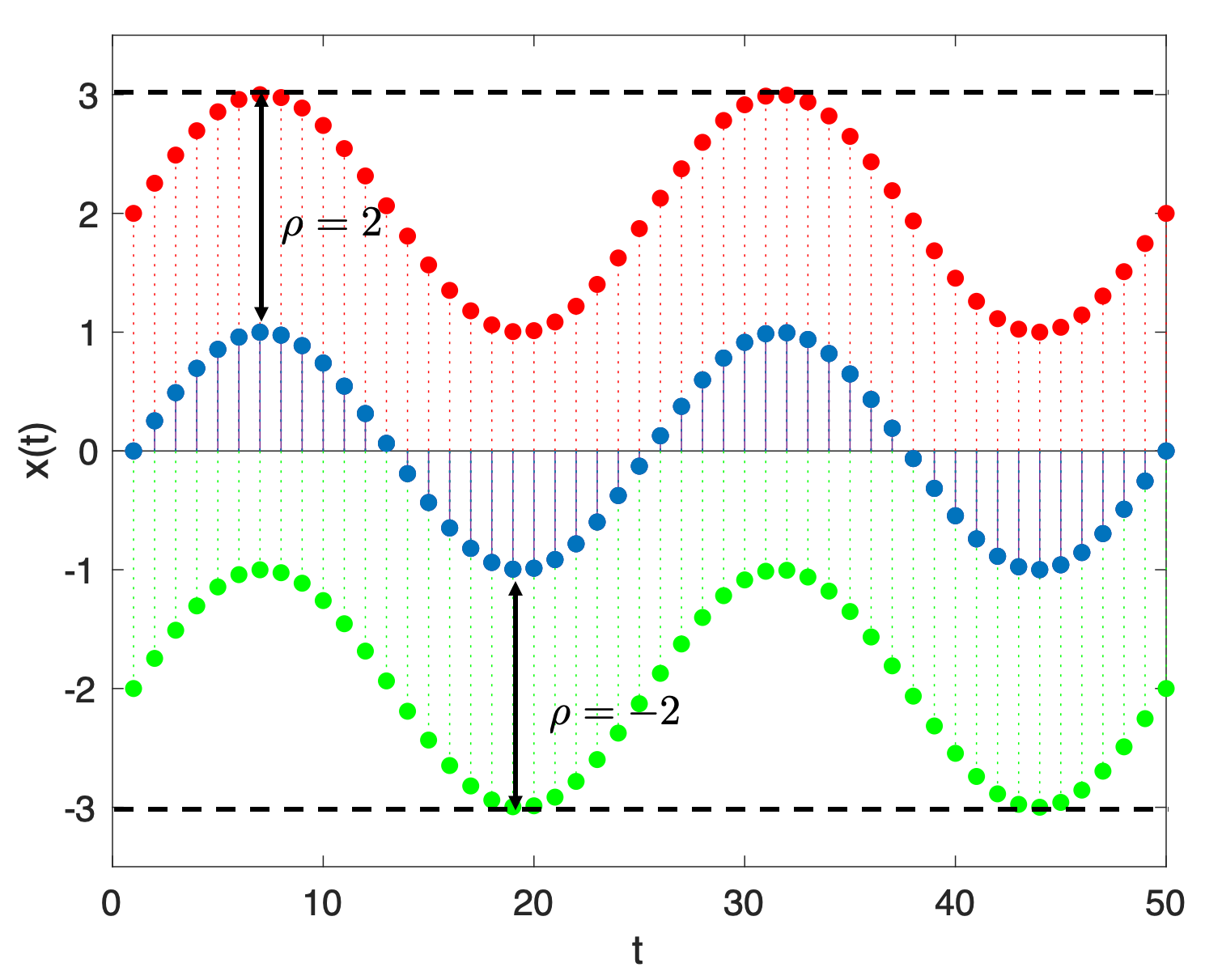
Figure 1: The approximate signed distance between $\mathbf{x}(t)$ (blue sinusoidal trace) and traces marginally violating $\varphi_{1}$ (i.e. the red trace) is $2$ (i.e. $\rho(\varphi_{1},x,0)=2$), and the approximate signed distance between $\mathbf{x}(t)$ and traces marginally satisfying $\varphi_{2}$ (i.e. the green trace) is $-2$ (i.e. $\rho(\varphi_{2},x,0)=-2$).

Parametric Signal Temporal Logic (PSTL).  Parametric STL (PSTL) [18] is an extension of STL where constants appearing in atomic predicates or time intervals are replaced by parameters. PSTL assumes a finite supply of parameter variables $\mathcal{P}$, which come from two distinct sets: value-domain parameter variables $\mathcal{P}_{V}$ and time-domain parameter variables $\mathcal{P}_{T}$. We assume that the parameters in $\mathcal{P}_{V}$ can take values in the set $V$, and those in $\mathcal{P}_{T}$ can take values in $T$. Then, the parameter space of the PSTL formula is $V\times T$. For any PSTL formula, we associate a valuation function $\nu$ that maps parameter variables to some value in the parameter space. Essentially, the valuation function has the effect of mapping a PSTL formula to an STL formula with a specific valuation for the parameters.

Example 2.2.

The property “Always for the first $\tau$ seconds, the trace $\mathbf{x}(t)$ is greater than some value $c_{1}$ and the signal $\mathbf{y}(t)$ is less than $c_{2}$” is written in PSTL as:

$$\varphi(c_{1},c_{2},\tau)=\mathbf{G}_{[0,\tau]}(x>c_{1}\,\wedge\,y<c_{2}).$$

In the above, $c_{1}$ and $c_{2}$ are value-domain parameter variables, and $\tau$ is a time parameter variable. Let $c_{1}\in[1,2]$, $c_{2}\in[0,3)$ and $\tau\in[0,10]$, the parameter space of $\varphi$ is $[1,2]\times[0,3)\times[0,10]$. The STL formula $\mathbf{G}_{[0,6]}(x>1.7\,\wedge\,y<2)$ is obtained with the valuation $\nu=\left\{\tau\mapsto 6,c_{1}\mapsto 1.7,c_{2}\mapsto 2\right\}$ applied to $\varphi$.

2.1 Requirements and Assumptions

In this section, we formalize the notion of output requirements and input or environment assumptions.

Definition 2.4 (Output requirement).

Output requirement or $\varphi_{\mathrm{out}}$ is an STL formula that is satisfied by output traces of the system if their behavior is desirable and is not satisfied otherwise.

Definition 2.5 (Environment Assumption).

Given a dynamical component model $M_{C}$ = $(\mathbf{u},\mathbf{x},\mathbf{y})$, an output requirement is an STL formula $\varphi_{\mathrm{out}}$, where $\mathsf{supp}(\varphi_{\mathrm{out}})=\mathbf{y}$. Given an output requirement $\varphi_{\mathrm{out}}$, an STL formula $\varphi_{\mathrm{in}}$ is called an environment assumption if:

1. $\mathsf{supp}(\varphi_{\mathrm{in}})=\mathbf{u}$,

2. $\forall\mathbf{u}(t):\left(\mathbf{u}(t)\models\varphi_{\mathrm{in}}\right)\implies\left(M(\mathbf{u}(t))\models\varphi_{\mathrm{out}}\right)$.

Essentially, an environment assumption is an STL property on the input traces to the model that guarantees that the corresponding output traces satisfy the output requirement $\varphi_{\mathrm{out}}$.

Example 2.3.

Consider a simple model $M$ that simply delays a given input signal by $1$ second, i.e. the value of the output at time $1$ is the value of the input signal at time $0$ (and the values of the output in times $[0,1)$ are defined as some default output trace value). Suppose the output requirement is $\mathbf{G}_{[1,100]}(\mathbf{y}>0)$, then the property $\mathbf{G}_{[0,99]}(\mathbf{u}>0)$ is a valid environment assumption for the model.

In software verification parlance, the environment assumption could be viewed as a pre-condition over the input trace to the model that guarantees an assertion on the output trace.

3 Environment Assumption Mining

In this section, we describe our overall approach to mine environment assumptions, and identify sub-problems that we will address in subsequent sections. The central idea in our approach is a counterexample-guided inductive synthesis (CEGIS) algorithm to mine environment assumptions. The key steps of this process are shown in Algorithm 1.

Input: Input signal domain $U$, Output requirement $\varphi_{\mathrm{out}}$, Input signal time domain $T(\mathbf{u})$, Model $M=(\mathbf{u},\mathbf{y})$, Simulation Budget $N$ for Falsification, Formula length limit $\ell_{\mathrm{max}}$, Classification Accuracy $1-\epsilon$

Output: Environment Assumption $\varphi_{\mathrm{in}}$

1 $\mathcal{T}$ = Sample input traces from $U$ using time instants from $T(\mathbf{u})$

2 foreach $\mathbf{u}(t)\in\mathcal{T}$ do

3       if $M(\mathbf{u}(t))\models\varphi_{\mathrm{out}}$ then  $\mathcal{T}_{\mathrm{good}}$ = $\mathcal{T}_{\mathrm{good}}\cup\{\mathbf{u}(t)\}$

4       else  $\mathcal{T}_{\mathrm{bad}}$ = $\mathcal{T}_{\mathrm{bad}}\cup\{\mathbf{u}(t)\}$

5      

6$\psi^{\mathrm{proposed}}$ = $\mathsf{EnumerateNextPSTL}()$

7 while $|\psi^{\mathrm{proposed}}|<\ell_{\mathrm{max}}$ do

8       (accuracy, $\Upsilon[\psi^{\mathrm{proposed}}]$) =   $\mathsf{DecisionTreeBasedSTLClassifier}(\psi^{\mathrm{proposed}},\mathcal{T}_{\mathrm{good}},\mathcal{T}_{\mathrm{bad}})$

9       $\varphi_{\mathrm{in}}^{\mathrm{proposed}}=\mathsf{GetSTL}(\Upsilon[\psi^{\mathrm{proposed}}])$

10       if accuracy $>1-\epsilon$ then

11             $\mathrm{cex}(t)$ = $\mathsf{Falsify}(\mathbf{y}\models\varphi_{\mathrm{out}},N)$

12              subject to $\mathbf{u}(t)\models\varphi_{\mathrm{in}}^{\mathrm{proposed}}$

13                   $\mathbf{y}(t)=M(\mathbf{u}(t))$

14             if $\mathrm{cex}(t)\neq\emptyset$ then  $\mathcal{T}_{\mathrm{bad}}$ = $\mathcal{T}_{\mathrm{bad}}\cup\{\mathrm{cex}(t)\}$

15             else  return $\varphi_{\mathrm{in}}^{\mathrm{proposed}}$

16            

17      else

18             $\psi^{\mathrm{proposed}}$ = $\mathsf{EnumerateNextPSTL}()$

19      

Algorithm 1 Environment Assumption Mining Algorithm

We assume that the user provides us a description of the input signal domain $U$ (i.e. upper and lower bounds on the values appearing in the input traces), as well as a set of time instants on which input traces are expected to be defined (i.e. $T(\mathbf{u})$). Initially, we randomly sample input traces (Line 1 and label them as good or bad (resp. Lines 1,1) depending on whether their corresponding outputs satisfy the given $\varphi_{\mathrm{out}}$. At the beginning of the while-loop, we assume that there is a PSTL formula $\psi^{\mathrm{proposed}}$ that is being considered as a candidate environment assumption. The first time the loop body is executed, this enumeration occurs in Line 1, otherwise a new PSTL formula is obtained in the loop in Line 1. Once we have a candidate PSTL formula $\psi^{\mathrm{proposed}}$, we use an off-the-shelf supervised learning approach to obtain a decision tree $\Upsilon[\psi^{\mathrm{proposed}}]$ from $\psi^{\mathrm{proposed}}$ using a procedure discussed in Sec. LABEL:sec:dt. We use a procedure described in Sec. LABEL:sec:dt2stl to obtain an interpretable STL formula $\varphi_{\mathrm{in}}^{\mathrm{proposed}}$ from $\Upsilon[\psi^{\mathrm{proposed}}]$. If $\varphi_{\mathrm{in}}^{\mathrm{proposed}}$ does not give a high classification accuracy for the given set of good/bad traces, we move to the next PSTL formula to be enumerated till we reach a user-defined upper bound on the maximum formula length. If we exceed this bound, our procedure fails to find an accurate environment assumption.

We note that it is possible that the candidate formula $\varphi_{\mathrm{in}}^{\mathrm{proposed}}$ while being accurate in classifying the set of traces in $\mathcal{T}_{\mathrm{good}}$ and $\mathcal{T}_{\mathrm{bad}}$ is too permissive. This means that it may allow for input traces not present in $\mathcal{T}_{\mathrm{good}}$ for which the corresponding output traces do not satisfy $\varphi_{\mathrm{out}}$. We wish to constrain the environment assumption to exclude such signals. Thus, we invoke an off-the-shelf falsification technique using the $\mathsf{Falsify}$ function to refine the synthesized environment assumption. There are many promising falsification tools such as [19, 20, 21] that our technique could use. The falsifier uses a global optimizer to identify an input trace $\mathbf{u}(t)$ satisfying $\varphi_{\mathrm{in}}^{\mathrm{proposed}}$ for which $M(\mathbf{u}(t))$ $\not\models\varphi_{\mathrm{out}}$ (Line 2). Typical falsifiers parameterize the input trace using a finite number of control points, i.e., time points at which the signal value is deemed to be an optimization variable. At all other time points, the intermediate signal values are obtained through a user-specified interpolation scheme. Let $\hat{\mathbf{u}}$ denote the control point vector used by the falsifier to generate the input trace $\mathbf{u}(t)$. Then, consider an optimizer that tries to minimize the following cost function: $$\mathrm{cost}(\hat{\mathbf{u}})=(\max(0,-\rho(\varphi_{\mathrm{in}}^{\mathrm{proposed}},\mathbf{u},0))+1)^{2k}-1+\rho(\varphi_{\mathrm{out}},\mathbf{y},0)$$

Essentially, this cost function represents a quantity that is highly positive if the input trace does not satisfy $\varphi_{\mathrm{in}}^{\mathrm{proposed}}$, thus favoring input control point vectors leading to traces that satisfy $\varphi_{\mathrm{in}}^{\mathrm{proposed}}$. The constant $k$ is a positive integer chosen to overpower the maximum negative robustness that can result from the output trace $\mathbf{y}(t)$ not satisfying $\varphi_{\mathrm{out}}$. If the input does satisfy $\varphi_{\mathrm{in}}^{\mathrm{proposed}}$, the first term is simply $0$, and we only look for outputs that violate $\varphi_{\mathrm{out}}$.

If such an input trace is found, we add it to the list of bad traces (Line 1), and restart the enumerative solver from the last formula that it had enumerated (Line 1). If there is no counterexample found, the algorithm terminates with an STL formula representing the environment assumption. Note that our algorithm automatically learns the structure of the environment assumption as well as the parameter values. In the following sections, we will explain the procedure for the decision tree based learning of the classifier.

Remark 1.

A key step in Algorithm 1 is systematic enumeration of PSTL formulas. This procedure covers the space of all PSTL formulas. We omit the details of how this is performed, but in essence, the procedure closely mimics the work in [22]. Longer formulas are constructed from smaller formulas in a systematic fashion by defining a canonical order in which STL operators are used, and certain efficiency improvements are added to avoid enumerating semantically equivalent formulas with different syntax trees. More details about systematic enumeration is provided in Appendix.

4 Supervised Learning of STL classifiers

In this section we explain our decision-tree based algorithm for learning the parameter valuations of a PSTL formula that yields an accurate STL classifier. Before delving into the details of our procedure, we recall some related work on supervised learning of STL formulas from data. In [22], the authors consider a technique that enumerates monotonic PSTL templates and then uses the validity domain boundary of the PSTL formula to classify traces.

Definition 4.1 (Monotonic PSTL).

Consider a PSTL formula $\varphi(\mathbf{p})$ where $\mathbf{p}=(p_{1},\ldots,p_{m})$. Let $\nu(\mathbf{p})$ and $\nu^{\prime}(\mathbf{p})$ be two valuations which assign identical values to all parameters except $p_{i}$. The formula $\varphi(\mathbf{p})$ is called monotonically increasing in $p_{i}$ if for all traces $\mathbf{x}(t)$, if $\mathbf{x}(t)\models\varphi(\nu(p_{i}))$ and $\nu(p_{i})<\nu^{\prime}(p_{i})$, then it implies that $\mathbf{x}(t)\models\varphi(\nu^{\prime}(p_{i}))$. A monotonically decreasing PSTL formula can be defined analogously. A PSTL formula is called monotonic in a parameter $p_{i}$ if it is either monotonically increasing or decreasing, and is called monotonic if it is monotonic in each of its parameters.

Example 4.1.

The formula $\mathbf{G}_{[0,10]}(\mathbf{x}<c)$ is monotonically increasing in $c$, because once it is true for a given trace for some value $\nu(c)$ of $c$, it will be true for all values greater than $\nu(c)$.

Definition 4.2 (Validity Domain, Validity Domain Boundary).

The validity domain $\mathcal{V}(\varphi)$ is an open subset of ${\mathcal{D}_{\mathcal{P}}}$ s.t.: $\forall\nu(\mathbf{p})\in\mathcal{V}(\varphi)$, and for all traces $\mathbf{x}(t)$, $\mathbf{x}(t)\models\varphi(\nu(\mathbf{p}))$. The boundary of the validity domain is the set difference between the closure of the validity domain and its interior.

Example 4.2.

Consider a set of traces $\mathbf{x}(t)$ that are all bounded above by $1$, then for the formula $\mathbf{G}_{[0,10]}(\mathbf{x}<c)$, the validity domain is the set $(1,\infty)$, and the validity domain boundary is the single point $c=1$.

In general, computing even the validity domain boundary of a PSTL formula where the atomic predicates are linear inequalities of the signals requires reasoning over semi-linear sets [18]. Thus, in [23], the authors have proposed a multi-dimensional binary search algorithm to approximate the validity domain boundary. In [22], the authors propose combining the algorithm from [23] with a supervised learning procedure. Essentially, each step in [23] identifies a set of points in the parameter space that lie on the validity domain boundary. In [22], the authors propose using each successive set of points discovered by the algorithm to define a classifier. The procedure terminates when a sufficiently high accuracy classification is obtained. A key limitation of this approach is that it only works for monotonic PSTL formulas, and when the number of parameters is high, computing the validity domain boundary can be time-consuming.

Instead, in this paper, we consider an approach based on sampling the parameter space, obtaining robustness values for a given set of “seed” traces at each of the sampled points, and using these values as features in a decision-tree based classification algorithm. We now explain each of these steps in detail.

4.1 Decision Tree based Supervised Learning

Decision trees are a non-parametric supervised learning method used for classification and regression. Learned trees can also be represented as sets of if-then else rules which are understandable by humans. The depth of a decision tree is the length of the longest path from the root to the leaf nodes, and the size of a decision tree is the number of nodes in the tree. A binary decision tree is a tree that every non-terminal node has at most two children. Decision trees represent a disjunction of conjunctions of constraints represented by nodes in the tree. Each path from the tree root to a leaf corresponds to a conjunction of constraints while the tree itself is a disjunction of these conjunctions [24].

While decision trees improve human readability [24], they are not specialized in learning temporal properties of timed traces. A naïve application of a decision tree to timed traces would treat every time instant in the trace as a decision variable, leading to deep trees that lose interpretability.

Example 4.3.

We applied decision trees on a 2-dimensional synthetic data set. The data set consists of two sets of traces corresponding to signals $x$ and $y$. In both sets $y(t)=x(t-d)$, which $d$ represents the delay between $x$ and $y$. For label $1$ traces $d<20$, and for label $0$ traces $d>30$. Each node in decision tree corresponds a point of $x$ and $y$ signals in time. Decision trees failed to classify the data set properly since the resulting tree has $179$ nodes, and the accuracy of training is $50\%$, which is the accuracy of random classification. On the other hand, this data set can be easily classified using STL formula $\varphi=G_{[0,100]}(x(t)\geq 0.1\implies F_{[0,20)}(y(t)\geq 0.1))$. A naïve use of decision trees thus does not provide the same dynamic richness as many temporal logic formulas.

Feature selection in decision trees is challenging; in our work, we use robustness values of a given PSTL formula at different parameter valuations as features. For a PSTL formula containing only one parameter this is unnecessary, as we can simply determine the validity domain boundary (corresponding to $0$ robustness value) by a simple binary search. However, for PSTL formulas with multiple independent parameters, random samples of the parameter space can be informative about the validity domain boundary and hence serve as features for our decision-tree based learning algorithm. Formally, Algorithm 2 assumes that we are given sets of traces $\mathcal{T}_{\mathrm{good}}$ and $\mathcal{T}_{\mathrm{bad}}$, a PSTL formula $\psi(\mathbf{p})$ (with the parameter space ${\mathcal{D}_{\mathcal{P}}}$). The algorithm returns the classification accuracy and the decision tree produced by an off-the-shelf decision tree learning algorithm.

Input: $\psi,\mathcal{T}_{\mathrm{good}},\mathcal{T}_{\mathrm{bad}}$

Output: accuracy, $\Upsilon[\psi]$

1 Function $\mathsf{DecisionTreeBasedSTLClassifier}(\psi,\mathcal{T}_{\mathrm{good}},\mathcal{T}_{\mathrm{bad}})$:

       // Split data for train and test

2       $\mathcal{T}_{\mathrm{train}},\mathcal{T}_{\mathrm{test}}$ $\leftarrow$ $\mathsf{split}(\mathcal{T}_{\mathrm{good}}\cup\mathcal{T}_{\mathrm{bad}},0.7)$

3      

      // Compute robustness values as features for training

4       $\mu_{\mathrm{train}}$ $\leftarrow$ $\mathsf{computeFeatures}(\mathcal{T}_{\mathrm{train}},\psi,{\mathcal{D}_{\mathcal{P}}}(\psi))$

5       foreach $\mathbf{u}(t)\in(\mathcal{T}_{\mathrm{test}}\cup\mathcal{T}_{\mathrm{train}})$ do

6             $\ell(\mathbf{u}(t))$ $\leftarrow$ $(\mathbf{u}(t)\in\mathcal{T}_{\mathrm{good}})$

7      

      // Train decision tree using computed features

8       $\Upsilon[\psi^{\mathrm{proposed}}]$ $\leftarrow$ $\mathsf{TrainDecisionTree}(\mu,\ell(\mu))$

9      

      // Compute accuracy

10       foreach $\mathbf{u}(t)\in\mathcal{T}_{\mathrm{test}}$ do

11             $\mu_{\mathrm{test}}(\mathbf{u}(t))$ $\leftarrow$ $\mathsf{computeFeatures}(\mathcal{T}_{\mathrm{test}},\psi,{\mathcal{D}_{\mathcal{P}}}(\psi))$

12             $\ell^{\prime}(\mathbf{u}(t))$ $\leftarrow$ $\Upsilon[\psi^{\mathrm{proposed}}](\mu_{\mathrm{test}}(\mathbf{u}(t)))$

13      accuracy $\leftarrow$ $\mathsf{computeAccuracy}(\ell,\ell^{\prime})$

14       return accuracy, $\Upsilon[\psi]$

15      

16Function $\mathsf{computeFeatures}(\mathcal{T},\psi,{\mathcal{D}_{\mathcal{P}}}(\psi))$:

       // Sample $m$ parameter values

17       ${\mathcal{D}_{\mathcal{P}}}_{m}\leftarrow\mathsf{gridSample}({\mathcal{D}_{\mathcal{P}}},m)$

18       foreach $\mathbf{u}(t)\in\mathcal{T}$ do

19             for $i\in[1,m]$ do

20                   $\psi_{i}$ $\leftarrow$ $\psi(\nu({\mathcal{D}_{\mathcal{P}}}_{m}(i)))$

21                   $\mu(\mathbf{u}(t))[i]$ $\leftarrow$ $\rho(\psi_{i},\mathbf{u},0)$ ;

22            

23      return $\mu$

24      

Algorithm 2 Classification using decision trees

In Line 2, we split the given set of traces into training and test sets; $0.7$ is an arbitrary heuristic indicating the ratio of the size of the training set to the total number of traces. In Line 2, we invoke the function $\mathsf{computeFeatures}$. Essentially, this function maps each trace $\mathbf{u}(t)$ in the set $\mathcal{T}_{\mathrm{train}}$ to a $m$-element feature vector $\mu(\mathbf{u}(t))$. To produce this vector, we obtain $m$ samples of the parameter space along a user-defined grid. Note that the grid sampling procedure also checks for validity of a parameter sample; e.g. if $\tau_{1}$ and $\tau_{2}$ are parameters belonging to the same time-interval $[\tau_{1},\tau_{2}]$, then it imposes that $\tau_{1}<\tau_{2}$. See Fig. 2 for an example of grid sampling. Each sample in the parameter space corresponds to a valuation for the parameters in the PSTL formula $\psi$, and applying the $i^{th}$ valuation yields the STL formula $\psi_{i}$ (Line 2). We then use the robustness value of $\mathbf{u}(t)$ w.r.t. $\psi_{i}$ as the $i^{th}$ element of the feature vector, i.e. $\mu(\mathbf{u}(t))[i]$. For each trace in the set $\mathcal{T}_{\mathrm{train}}$ and $\mathcal{T}_{\mathrm{test}}$ , we assign it label $1$ if it belongs to $\mathcal{T}_{\mathrm{good}}$, and $0$ otherwise (Line 2).

In Line 2, we invoke the decision tree procedure on the feature vectors and the label sets. The edge between any node in the decision tree $\Upsilon[\psi]$ and its children is annotated by a constraint of the form $\rho(\psi_{i},\mathbf{u},0)<c$ for the left child, and its negation for the right child. Here, $c$ is some real number. We give further details on the structure of the tree in the Section LABEL:sec:dt2stl. Next, we compute the accuracy of the decision tree by computing the labels of the traces in the test set $\mathcal{T}_{\mathrm{test}}$ and comparing them to their ground truth labels. The function $\mathsf{computeAccuracy}$ simply computes the ratio $|\{\mathbf{u}(t)\mid\ell(\mathbf{u}(t))=\ell^{\prime}(\mathbf{u}(t))\}|\,/\,|\mathcal{T}_{\mathrm{test}}|$.

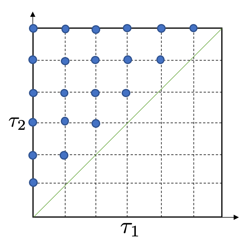
Figure 2: Grid sampling of time parameters for formula $\mathbf{G}_{[\tau_{1},\tau_{2}]}(x(t)>c)$. Since $\tau_{1}$ should be less than $\tau_{2}$, the area above $\tau_{1}=\tau_{2}$ line (green line) is sampled.

5 Extracting Interpretable STL formulas

Figure 3: Example Tree returned by $\mathsf{DecisionTreeBasedSTLClassifier}$

The function $\mathsf{DecisionTreeBasedSTLClassifier}$ described in Algo. 2 returns a decision tree $\Upsilon[\psi]$ of the form shown in Fig. 3. We note that the edge labels correspond to inequality tests over STL formulas $\psi_{i}$ corresponding to the same PSTL formula $\psi$, but with different valuations for the parameters. Each path from the root of the tree to a leaf node represents a conjunction of the edge labels, and the disjunction over all paths leading to the same label represents the symbolic condition for mapping a given trace to a given label. Paths leading to label $\ell=1$ correspond to the environment assumption that we wish to mine. We now show that given a decision tree of this form, it is always possible to extract an STL formula from the symbolic condition that the decision tree represents.

Lemma 5.1.

For any STL formula $\varphi$, any trace $\mathbf{u}(t)$, and any time instance $t$, for $\sim\in\{<,\geq,>,\leq\}$, any constraint of the form $\rho(\varphi,\mathbf{u},t)\sim c$ can be transformed to the satisfaction or violation of a formula $\hat{\varphi}$ by $\mathbf{u}(t)$, where $\hat{\varphi}$ can be obtained from $\varphi$ and $c$ using simple transformations (shifts in space parameters).

Proof.

We prove the above lemma using structural induction on the syntax of STL. The base case is for atomic predicates. Suppose $\varphi=f(\mathbf{u})>c$, then if $\rho(\varphi,\mathbf{u},t)>c$, by the definition of a robustness value, $f(\mathbf{u}(t))-(c+c)>0$. Let $\hat{\varphi}=f(\mathbf{u})>(c+c)$. Then, $\rho(\varphi,\mathbf{u},t)>c$ implies that at time $t$, $\mathbf{u}(t)\models\hat{\varphi}$. The proof for atomic predicates indicating other kinds of inequalities is similar.

The inductive hypothesis is that the above lemma holds for all proper subformulas of $\varphi$, and in the inductive step we show that if this is true, then the lemma holds for $\varphi$. (1) Let $\varphi=\neg\psi$. Then, $\rho(\neg\psi,\mathbf{u},t)>c$ implies that $-\rho(\psi,\mathbf{u},t)>c$, or $\rho(\psi,\mathbf{u},t)\leq-c$. Let $c^{\prime}=-c$, then by the inductive hypothesis, there is a formula $\hat{\psi}$ such that $\rho(\hat{\psi},\mathbf{u},t)\leq 0$.

(2) Let $\varphi=\psi_{1}\wedge\psi_{2}$. If $\rho(\psi_{1}\wedge\psi_{2},\mathbf{u},t)>c$, then $\min(\rho(\psi_{1},\mathbf{u},t),\rho(\psi_{2},\mathbf{u},t))>c$, which implies that $\rho(\psi_{1},\mathbf{u},t)>c$ and $\rho(\psi_{2},\mathbf{u},t)>c$. Again, by the inductive hypothesis, this implies that there are formulas $\hat{\psi_{1}}$ and $\hat{\psi_{2}}$ such that $\rho(\hat{\psi_{1}},\mathbf{u},t)>0$ and $\rho(\hat{\psi_{2}},\mathbf{u},t)>0$. This implies that $\min(\rho(\hat{\psi_{1}},\mathbf{u},t),\rho(\hat{\psi_{2}},\mathbf{u},t))>0$, or $\rho(\hat{\psi_{1}}\wedge\hat{\psi_{2}},\mathbf{u},t)>0$.

(3) Let $\varphi=\psi_{1}\vee\psi_{2}$. An argument similar to (2) can be used to prove that we can obtain $\hat{\psi_{1}}$ and $\hat{\psi_{2}}$ such that $\rho(\hat{\psi_{1}}\vee\hat{\psi_{2}},\mathbf{u},t)>0$.

(4) Let $\varphi$ = $\mathbf{G}_{I}\psi$. $\rho(\mathbf{G}_{I}\psi,\mathbf{u},t)>c$ implies that $\forall t^{\prime}\in t\oplus I$, $\rho(\psi,\mathbf{u},t)>c$. Following similar reasoning as (2), and using the inductive hypothesis, we can show that there exists an STL formula $\hat{\psi}$ such that the above is equivalent to $\rho(\mathbf{G}_{I}\hat{\psi},\mathbf{u},t)>0$.

(5) For $\varphi$ = $\mathbf{F}_{I}\psi$, and $\varphi=\psi_{1}\mathbf{U}_{I}\psi_{2}$ similar reasoning as (4) can be used. We omit the details for brevity.

Finally, we can have a similar proof for any constraint of the form $\rho(\varphi,\mathbf{u},t)<c$. For example, consider $\varphi=\psi_{1}\wedge\psi_{2}$. $\rho(\varphi,\mathbf{u},t)<c$ implies that $\min(\rho(\psi_{1},\mathbf{u},t),\rho(\psi_{2},\mathbf{u},t))<c$, which in turn implies that $\rho(\psi_{1},\mathbf{u},t)<c$ or $\rho(\psi_{2},\mathbf{u},t)<c$. By the inductive hypothesis we can obtain $\hat{\psi_{1}}$ and $\hat{\psi_{2}}$ such that $\rho(\hat{\psi_{1}},\mathbf{u},t)<0$ or $\rho(\hat{\psi_{2}},\mathbf{u},t)<0$, which implies that $\rho(\hat{\psi_{1}}\wedge\hat{\psi_{2}},\mathbf{u},t)<0$.

As we are able to prove the inductive step for any kind of STL operator, and for all types of constraints on the robustness value, by combining the different cases, we can conclude that the lemma holds for an arbitrary STL formula. ∎

Theorem 1.

Given a decision tree $\Upsilon[\psi]$ where edge labels denote constraints of the form $\rho(\psi_{i},\mathbf{u},0)>c_{i}$, we can obtain an STL formula that is satisfied by all input traces that are labeled $1$ by the decision tree.

Proof.

The proof follows from the proof of Lemma 5.1. Essentially, each constraint corresponding to an edge label can be transformed into an equivalent STL formula, and each path is a conjunction of edge labels; so each path gives us an STL formula representing the conjunction of formulas corresponding to each edge label. Finally, a disjunction over all paths corresponds to a disjunction over formulas corresponding to each path. ∎

Remark 2.

We note that the above procedure does not require the PSTL formula to be monotonic. If the chosen PSTL formula is monotonic, then it is possible to simplify the formula further. Essentially, along any path, we can retain only those formulas corresponding to parameter valuations that are incomparable according to the order imposed by monotony. Furthermore, each of these valuations corresponds to points on the validity domain boundary as the robustness value for these valuations is close to zero. We also remark that Lemma 5.1 gives us a constructive approach to build an STL formula from the decision tree – we simply need to follow the recursive rules to push the constants appearing in the inequalities on the robustness values to the atomic predicates.

6 Benchmarking Supervised Learning

We divide our evaluation of the techniques presented in this paper into two parts. In this section, we primarily benchmark the efficacy of our decision tree based supervised learning approach. In the next section, we discuss case studies of mining environment assumptions using a combination of enumerative structure learning of the PSTL formula with the decision tree based classification approach. We run the experiments on an Intel Core-i7 Macbook Pro with 2.7 GHz processors and 16 GB RAM and used decision tree algorithms from Statistics and Machine Learning Toolbox in Matlab with default parameters.

Maritime Surveillance.  We compare the results of classification with our tool with the DTL4STL tool [25]. For a fair comparison, we use the same data set used by [25]. The maritime surveillance data set is a 2-dimensional synthetic data set consists of three types of behaviors: one normal and two anomalous behaviors (see Fig. 4).

We applied our tool to 600 traces from this data set (300 traces for training and 300 traces for testing). The STL formulas learned by our technique are as follows:

$$\varphi_{green}=\neg\varphi_{1}\,\wedge\,\varphi_{2}$$

$$\varphi_{blue}=\neg\varphi_{2}$$

$$\varphi_{red}=\varphi_{1}\,\wedge\,\varphi_{2},$$

where $\varphi_{1}=\mathbf{G}_{[15,30]}(x(t)<39)$ and $\varphi_{2}=\mathbf{G}_{[30,45]}(x(t)<41.98)$. $\varphi_{green}$ is the formula for classification of green traces from the others (red and blue traces). $\varphi_{blue}$ and $\varphi_{red}$ classify blue and red traces from the others respectively. The train accuracy is $100\%$ and, the test accuracy is $99\%$ with training time = 24.82 seconds.The simplest STL formula learned by DTL4STL [25] to classify green traces from the others is:

$$\varphi=(\varphi_{1}\,\wedge\,(\neg\varphi_{2}\vee(\varphi_{2}\,\wedge\,\neg\varphi_{3})))\vee(\neg\varphi_{1}\,\wedge\,(\varphi_{4}\,\wedge\,\varphi_{5}))$$

$$\varphi_{1}=\mathbf{G}_{[199.70,297.27)}(\mathbf{F}_{[0.00,0.05)}(x[t]\leq 23.60)$$

$$\varphi_{2}=\mathbf{G}_{[4.47,16.64)}(\mathbf{F}_{[0.00,198.73)}(y[t]\leq 24.20)$$

$$\varphi_{3}=\mathbf{G}_{[34.40,52.89)}(\mathbf{F}_{[0.00,61.74)}(y[t]\leq 19.62)$$

$$\varphi_{4}=\mathbf{G}_{[30.96,37.88)}(\mathbf{F}_{[0.00,250.37)}(x[t]\leq 36.60)$$

$$\varphi_{5}=\mathbf{G}_{[62.76,253.23)}(\mathbf{F}_{[0.00,41.07)}(y[t]\leq 29.90)$$

with the average misclassification rate of $0.007$. This STL formula is long and complicated compared to the STL formula $\varphi_{green}$ learned by our framework. Long formulas hinder interpretability and are not desirable for describing time-series behaviors. The reason behind generating complicated formulas by DTL4STL [25] is the restriction to only eventually and globally as PSTL templates. Our technique considers the space of all PSTL formulas in increasing order of complexity which results in simple and interpretable STL classifiers.

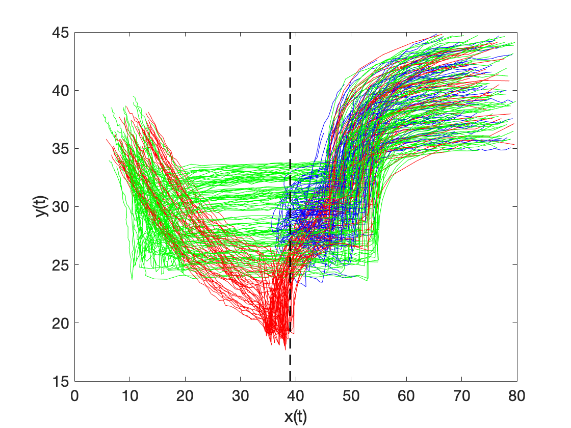
Figure 4: Naval surveillance data set [25](Green traces: normal trajectories, red and blue traces: two kinds of anomalous trajectories and the dashed line indicates one of the space parameters learned by our procedure.

ECG5days.  We also applied our technique on ECG five days data set from the UCR time-series repository [26]. The data set consists of echo-cardiogram signals recorded from a 67 year old male. The two classes correspond to two dates that the ECG was recorded, which are five days apart. We used 300 traces from this data set for training and 300 for testing. The STL formula learned by our method to classify two classes of ECG behaviors is:

$$\varphi=\neg\varphi_{1}\wedge(\varphi_{2}\vee\neg\varphi_{3})$$

$$\varphi_{1}=\mathbf{G}_{[19.28,57.86]}(\mathbf{F}_{[19.28,38.57]}(x[t]>0.48)$$

$$\varphi_{2}=\mathbf{G}_{[38.57,57.86]}(\mathbf{F}_{[19.28,57.86]}(x[t]>1.87)$$

$$\varphi_{3}=\mathbf{G}_{[38.57,57.86]}(\mathbf{F}_{[19.28,57.86]}(x[t]>1.32)$$

with training accuracy = $99\%$ and testing accuracy = $96\%$. The required time for training is 1449.34 seconds.

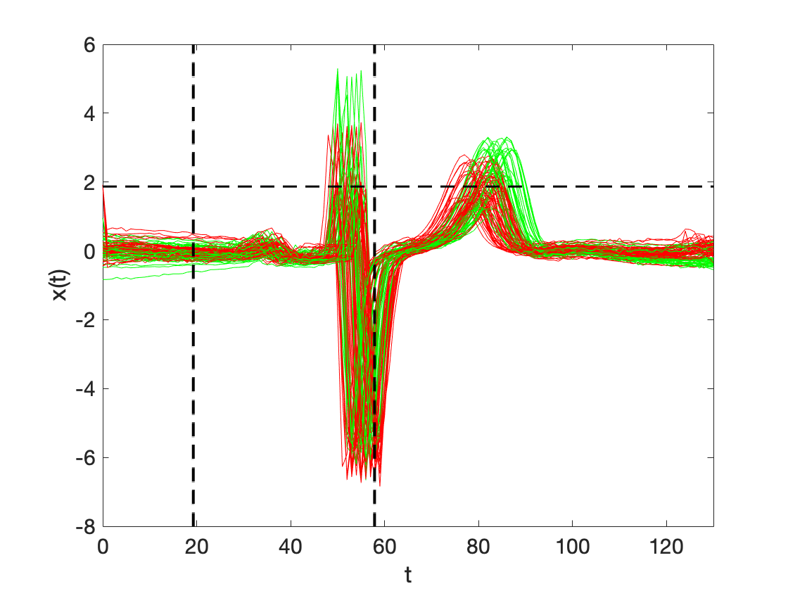
Figure 5: ECG five days data set from UCR time-series repository [26]. The two classes correspond to two dates that the ECG signals were recorded. Dash lines illustrate the time and space parameters of the learned STL formula.

7 Case Studies

In this section, we benchmark mining environment assumptions on a few case studies. The first is a synthetic model that we hand-crafted to demonstrate learning STL assumptions. The second is a model of an automatic transmission system. A model of abstract fuel control is considered as the third case study.

7.1 Synthetic model

Simulink^®is a visual block diagram language commonly used in industrial settings to model component-based CPS designs. We created a Simulink^®model of an oscillator component that has two input signals $u_{1}$ and $u_{2}$ and an output signal $y$. The model has an internal flag that is turned on if within $3$ seconds of the input value $u_{1}$ falling below $0$, the input value $u_{2}$ also falls below $0$. When the flag is turned on, the oscillator outputs a sinusoidal wave with amplitude $5$ units, and outputs a sine wave with amplitude $1$ unit otherwise. We imagine a scenario where a downstream component requires the output of the oscillator component to be bounded by $[-1,1]$. I.e., we require that the output $y$ satisfies the STL requirement $\varphi_{\mathrm{out}}=\mathbf{G}(-1\leq y(t)\leq 1)$.

In this example, we generate a large number of input traces using a $Simulink\textsuperscript{\textregistered}$ based signal generator. We pick a small subset of these traces that includes input traces that both lead to outputs satisfying $\varphi_{\mathrm{out}}$ (i.e. the good traces), and violating $\varphi_{\mathrm{out}}$ (bad traces). We use our supervised learning framework to learn an STL classifier $\varphi_{\mathrm{in}}$. We then invoke the counterexample-guided refinement step of Algorithm 1 to improve $\varphi_{\mathrm{in}}$. We learned the environment assumption $\varphi_{\mathrm{in}}=\mathbf{G}_{[0,20]}(u_{1}(t)<0\implies\mathbf{G}_{[0,5]}(u_{2}(t)\geq 0))$. This means that when input $u_{1}$ becomes negative, $u_{2}$ should stay non-negative within $[0,5]$ seconds. Otherwise, the output will violate $\varphi_{\mathrm{out}}$. The time taken to learn this $\varphi_{\mathrm{in}}$ is 6084 seconds and the training and testing accuracies are $100\%$ respectively. We note that in this case, the learned formula $\varphi_{\mathrm{in}}$ is stronger than the theoretical environment assumption that we had in mind when designing the model. This discrepancy can be due to the reason that our training set did not include trajectories where $u_{1}(t_{1})<0$ and $u_{2}(t_{2})<0$ occurred when $3<t_{2}-t_{1}<5$.

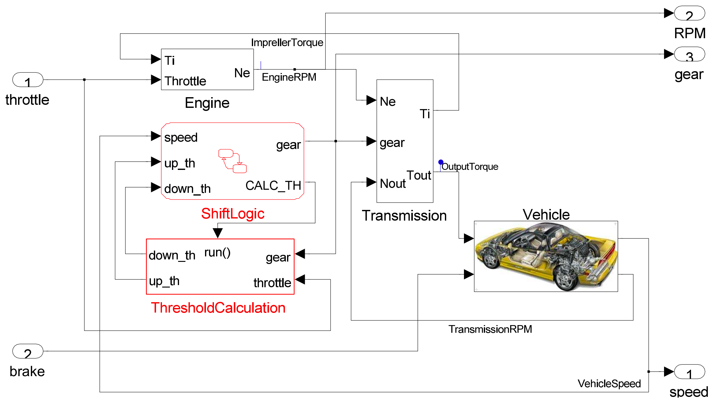
Figure 7: The Simulink model of automatic transmission controller. Inputs of the system are throttle and brake. RPM, gear and speed are outputs of the system.

Automatic Transmission Controller.  We consider automatic transmission controller which is a built-in model in Simulink^®, shown in Fig. 7 in Appendix. This model consists of modules to represent the engine, transmission, the vehicle, and a shift logic block to control the transmission ratio. User inputs to the model are throttle and brake torque. Engine speed, gear and vehicle speed are outputs of the system. We are interested in the following signals: the throttle, the vehicle speed, and the engine speed measured in RPM (rotations per minute). We wish to mine the environment assumptions on the throttle that ensures that the engine speed never exceeds 4500 rpm, and that the vehicle never drives faster than 120 mph. In other words, we want to mine the STL specification $\varphi_{\mathrm{in}}$ on input of the system (throttle) that results in meeting the following output requirement:

$$\varphi_{\mathrm{out}}=\mathbf{G}(RPM\leq 4500)\,\wedge\,\mathbf{G}(speed\leq 120).$$

A set of traces that violate this requirement is shown in Fig. 6. We applied our assumption mining method on 600 throttle traces (300 for training and 300 for testing). The formula produced by our framework is $\varphi_{\mathrm{in}}=\mathbf{G}_{[240,480]}(x(t)<40.4281)$ with training and testing accuracy equal to $100\%$ and $98\%$ respectively. This formula implies that if the throttle stays below $40.4281$ in time interval $[240,480]$, the engine and vehicle speed will meet the requirement. Otherwise, engine or vehicle speed violate the specifications and go beyond the specified threshold. It is difficult to mine such behaviors by looking at input and output traces of the system, and our technique helped in mining such assumptions on input automatically. The training time for learning the STL formula is 28.18 seconds.

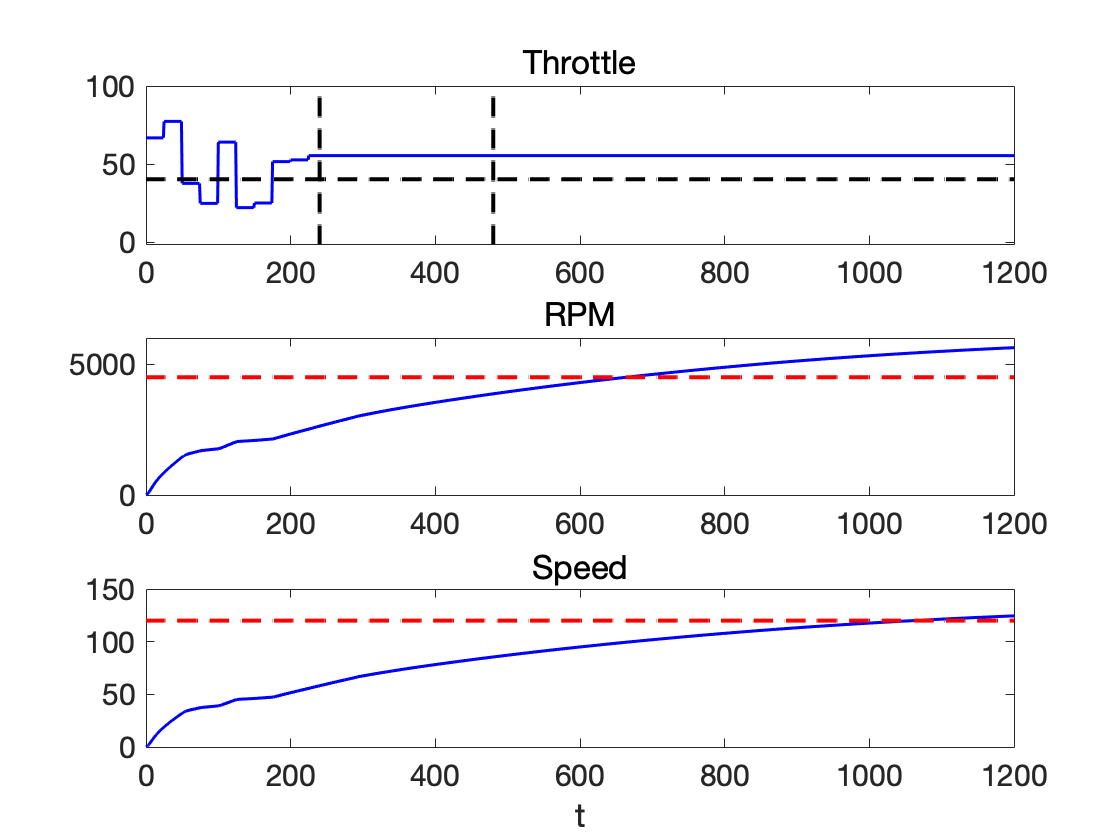
Figure 6: Violating traces for the automatic transmission controller.

Abstract Fuel Control Model.  In [7], the authors provide a $Simulink\textsuperscript{\textregistered}$ model for a power train control system. The model takes as input the throttle angle and engine speed, and outputs the Air-to-Fuel ratio. As specified in [7], the authors indicate that it is important for the A/F ratio to stay within $10\%$ of the nominal value. The output requirements in [7] are applicable only in the normal mode of operation of the model, when the throttle angle exceeds a certain threshold, the model switches into the power mode. In this mode, the A/F ratio is allowed to be lower. We wanted to extract the assumptions on the throttle angle that lead to significant excursions from the stoichiometric A/F value. We were able to learn the formula $\mathbf{G}_{[0,100]}(x(t)<61.167)$ which confirms that the excursions happen when the model goes into the power mode. We were able to synthesize the environment assumptions in 13.40 seconds with both training and test accuracy accuracy of $100\%$.

8 Related Work

Learning from timed traces.  In the machine learning (ML) community, various supervised learning methods for timed traces have been proposed. Traditionally, ML techniques rely on large sets of generic features (such as those based on statistics on the values appearing in the timed traces of features obtained through signal processing). A key drawback of ML approaches is the lack of interpretability of the classifiers.

Partially to address interpretability, there have been significant recent efforts at learning temporal logic formulas from data. There is work on learning STL formulas in a supervised learning context [25, 27, 28, 18, 11, 29, 30, 31], passive learning [32], an unsupervised learning context [15, 2, 1], and in an active learning setting [33]. Especially relevant to this paper is the seminal work in [25], where the authors propose learning the structure and parameters of STL formulas using decision trees. In contrast to our technique where there is a single STL formula used throughout the decision tree, in [25], each node is associated with a primitive PSTL formula. The technique then makes use of impurity measures to rank the primitives according to how accurately they label the set of traces (compared to ground truth). The primitives come from a fragment of PSTL containing formulas with only top-level $\mathbf{F}$, $\mathbf{G}$, $\mathbf{F}\mathbf{G}$ or $\mathbf{G}\mathbf{F}$ operators. We observe that the generated STL formulas in this approach can become long and complicated, especially because each node in the decision tree can potentially be a different STL formula. The decision trees produced by this method lead to formulas that splice together local deductions over traces together into a bigger formula.

Requirement Mining.  In [3, 34, 14], the authors address the problem of mining (output) requirements. Here, they assume that the structure of the PSTL formula representing an output requirement is provided by the user. The technique then uses counterexample guided inductive synthesis to infer formula parameters that result in an STL formula that is satisfied by all observed model outputs. Key differences from this method are: (1) we are interested in mining environment assumptions and not output requirements, (2) we use a supervised learning procedure that separates input traces that lead to outputs satisfying/violating an output requirement. The work in [35] focuses on mining temporal patterns from traces of digital circuits, and uses automata-based ideas that are quite different from the work presented here.

The seminal work proposed by Ferrère et al. [13] extends STL with support to define input-output interfaces. A new measure of input vacuity and output robustness is defined that better reflect the nature of the system and the specification intent. Then, the robustness computation is adapted to exploit the input-output interface and consequently provide deeper insights into the system behaviors. The connection of this work with our technique is that we also look at input-output relations using STL specifications. Our method mines a STL formula on input that guarantees a desired requirement on outputs. It would be interesting to extend the methods developed in this paper to the problem of mining interface-aware STL requirements. The latter is more expressive as it includes predicates that combine input and output variables, which our current paper does not address.

In [36], the authors analyze the falsifying traces of a cyber-physical system. Concretely, they seek to understand the properties or parts of the inputs to a system model that results in a counterexample using sensitivity analysis. They use learning methods (such as statistical hypothesis testing) from repeated simulations for the system under test. Tornado diagrams are used to find the values till no violation occurs while SMT solvers are used to find the falsifying intervals. Our work in this paper can be used to solve a similar problem, by basically mining environment assumptions for $\neg\varphi_{\mathrm{out}}$ for a given output requirement. A key difference in our technique is that we seek to explain falsifying input traces using an STL formula, while the work in [36] formulates explanations directly in terms of the input traces.

9 Conclusions

In this work, we addressed the problem of mining environment assumptions for CPS components and representing them using Signal Temporal Logic. An input trace satisfying an environment assumption is guaranteed to produce an output that meets the component requirement. We use a counterexample-guided procedure that systematically enumerates parametric STL formulas and uses a decision tree based classification procedure to learn both the structure and precise numeric constants of an STL formula representing the environment assumption. We demonstrate our technique on a few benchmark CPS models.

Appendix

Systematic enumeration [22].  From a grammar-based perspective a PSTL formula can be viewed as atomic formulas combined with unary or binary operators. For instance, PSTL formula $(x(t)>c_{1})\Rightarrow\mathbf{G}_{[0,\tau_{2}]}(x(t)<c_{2})$ consists of binary operator $\Rightarrow$, unary operator $\mathbf{G}$, and atomic predicates $x(t)>c_{1}$ and $x(t)<c_{2}$. Systematic enumeration algorithm consists of the following tasks:

1. First, basically, all formulas of length $1$, or parameterized signal predicates are enumerated.

2. All enumerated formulas are stored in a database sorted in non-decreasing order of their length.

3. Unary and Binary operators in a user-defined order are applied on all previously enumerated formulas.

4. As the space of all STL formulas is very large, and contains many semantically equivalent formulas, an optimization technique is proposed to prune the space of formulas considered.

For each PSTL formula $\psi^{\mathrm{proposed}}$ generated by Systematic enumeration algorithm [22], we apply the procedure which is formalized in Algo. 1. If $\psi^{\mathrm{proposed}}$ is a good environment assumption (high accuracy), algorithm terminates and $\psi^{\mathrm{proposed}}$ is returned. Otherwise, the procedure continues to generate new PSTL formulas.

References

- [1] Marcell Vazquez-Chanlatte, Jyotirmoy V Deshmukh, Xiaoqing Jin, and Sanjit A Seshia. Logical clustering and learning for time-series data. In International Conference on Computer Aided Verification, pages 305–325. Springer, 2017.
- [2] Marcell Vazquez-Chanlatte, Shromona Ghosh, Jyotirmoy V Deshmukh, Alberto Sangiovanni-Vincentelli, and Sanjit A Seshia. Time-series learning using monotonic logical properties. In International Conference on Runtime Verification, pages 389–405. Springer, 2018.
- [3] Xiaoqing Jin, Alexandre Donzé, Jyotirmoy V Deshmukh, and Sanjit A Seshia. Mining requirements from closed-loop control models. IEEE Transactions on Computer-Aided Design of Integrated Circuits and Systems, 34(11):1704–1717, 2015.
- [4] Pierluigi Nuzzo, Antonio Iannopollo, Stavros Tripakis, and Alberto L Sangiovanni-Vincentelli. From relational interfaces to assume-guarantee contracts. Technical report, UC Berkeley, 2014.
- [5] Jiwei Li, Pierluigi Nuzzo, Alberto Sangiovanni-Vincentelli, Yugeng Xi, and Dewei Li. Stochastic contracts for cyber-physical system design under probabilistic requirements. In Proceedings of the 15th ACM-IEEE International Conference on Formal Methods and Models for System Design, pages 5–14. ACM, 2017.
- [6] Tomoya Yamaguchi, Tomoyuki Kaga, Alexandre Donzé, and Sanjit A Seshia. Combining requirement mining, software model checking and simulation-based verification for industrial automotive systems. In 2016 Formal Methods in Computer-Aided Design (FMCAD), pages 201–204. IEEE, 2016.
- [7] Xiaoqing Jin, Jyotirmoy V Deshmukh, James Kapinski, Koichi Ueda, and Ken Butts. Powertrain control verification benchmark. In Proceedings of the 17th international conference on Hybrid systems: computation and control, pages 253–262. ACM, 2014.
- [8] Hendrik Roehm, Rainer Gmehlich, Thomas Heinz, Jens Oehlerking, and Matthias Woehrle. Industrial examples of formal specifications for test case generation. In Workshop on Applied veRification for Continuous and Hybrid Systems, ARCH@CPSWeek 2015, pages 80–88, 2015.
- [9] Bardh Hoxha, Houssam Abbas, and Georgios Fainekos. Benchmarks for temporal logic requirements for automotive systems. In Goran Frehse and Matthias Althoff, editors, ARCH14-15. 1st and 2nd International Workshop on Applied veRification for Continuous and Hybrid Systems, volume 34 of EPiC Series in Computing, pages 25–30. EasyChair, 2015.
- [10] James Kapinski, Xiaoqing Jin, Jyotirmoy Deshmukh, Alexandre Donzé, Tomoya Yamaguchi, Hisahiro Ito, Tomoyuki Kaga, Shunsuke Kobuna, and Sanjit Seshia. St-lib: a library for specifying and classifying model behaviors. Technical report, SAE Technical Paper, 2016.
- [11] Ezio Bartocci, Luca Bortolussi, and Guido Sanguinetti. Learning temporal logical properties discriminating ECG models of cardiac arrhytmias. arXiv preprint arXiv:1312.7523, 2013.
- [12] Fraser Cameron, Georgios Fainekos, David M Maahs, and Sriram Sankaranarayanan. Towards a verified artificial pancreas: Challenges and solutions for runtime verification. In Runtime Verification, pages 3–17. Springer, 2015.
- [13] Thomas Ferrère, Dejan Nickovic, Alexandre Donzé, Hisahiro Ito, and James Kapinski. Interface-aware signal temporal logic. In Proceedings of the 22nd ACM International Conference on Hybrid Systems: Computation and Control, pages 57–66. ACM, 2019.
- [14] Bardh Hoxha, Adel Dokhanchi, and Georgios Fainekos. Mining parametric temporal logic properties in model-based design for cyber-physical systems. International Journal on Software Tools for Technology Transfer, 20(1):79–93, 2018.
- [15] Austin Jones, Zhaodan Kong, and Calin Belta. Anomaly detection in cyber-physical systems: A formal methods approach. In 53rd IEEE Conference on Decision and Control, pages 848–853. IEEE, 2014.
- [16] Oded Maler and Dejan Nickovic. Monitoring temporal properties of continuous signals. In Formal Techniques, Modelling and Analysis of Timed and Fault-Tolerant Systems, pages 152–166. Springer, 2004.
- [17] Alexandre Donzé and Oded Maler. Robust satisfaction of temporal logic over real-valued signals. In Formal Modeling and Analysis of Timed Systems - 8th International Conference, FORMATS 2010, Klosterneuburg, Austria, September 8-10, 2010. Proceedings, pages 92–106, 2010.
- [18] Eugene Asarin, Alexandre Donzé, Oded Maler, and Dejan Nickovic. Parametric identification of temporal properties. In International Conference on Runtime Verification, pages 147–160. Springer, 2011.
- [19] Yashwanth Annapureddy, Che Liu, Georgios E Fainekos, and Sriram Sankaranarayanan. S-taliro: A tool for temporal logic falsification for hybrid systems. In TACAS, volume 6605, pages 254–257. Springer, 2011.
- [20] Jyotirmoy Deshmukh, Xiaoqing Jin, James Kapinski, and Oded Maler. Stochastic local search for falsification of hybrid systems. In International Symposium on Automated Technology for Verification and Analysis, pages 500–517. Springer, 2015.
- [21] Alexandre Donzé. Breach, a toolbox for verification and parameter synthesis of hybrid systems. In International Conference on Computer Aided Verification, pages 167–170. Springer, 2010.
- [22] Sara Mohammadinejad, Jyotirmoy V Deshmukh, Aniruddh G Puranic, Marcell Vazquez-Chanlatte, and Alexandre Donzé. Interpretable classification of time-series data using efficient enumerative techniques. arXiv preprint arXiv:1907.10265, 2019.
- [23] Oded Maler. Learning monotone partitions of partially-ordered domains (work in progress). 2017.
- [24] Thomas M. Mitchell. Machine Learning. McGraw-Hill, Inc., New York, NY, USA, 1 edition, 1997.
- [25] Giuseppe Bombara, Cristian-Ioan Vasile, Francisco Penedo, Hirotoshi Yasuoka, and Calin Belta. A decision tree approach to data classification using signal temporal logic. In Proceedings of the 19th International Conference on Hybrid Systems: Computation and Control, pages 1–10. ACM, 2016.
- [26] Yanping Chen, Eamonn Keogh, Bing Hu, Nurjahan Begum, Anthony Bagnall, Abdullah Mueen, and Gustavo Batista. The ucr time series classification archive. 2015.
- [27] Giuseppe Bombara and Calin Belta. Online learning of temporal logic formulae for signal classification. In 2018 European Control Conference (ECC), pages 2057–2062. IEEE, 2018.
- [28] Zhaodan Kong, Austin Jones, Ana Medina Ayala, Ebru Aydin Gol, and Calin Belta. Temporal logic inference for classification and prediction from data. In Proc. of HSCC, pages 273–282, 2014.
- [29] Laura Nenzi, Simone Silvetti, Ezio Bartocci, and Luca Bortolussi. A robust genetic algorithm for learning temporal specifications from data. In International Conference on Quantitative Evaluation of Systems, pages 323–338. Springer, 2018.
- [30] Ebru Aydin Gol. Efficient online monitoring and formula synthesis with past stl. In 2018 5th International Conference on Control, Decision and Information Technologies (CoDIT), pages 916–921. IEEE, 2018.
- [31] Ahmet Ketenci and Ebru Aydin Gol. Synthesis of monitoring rules via data mining. In 2019 American Control Conference (ACC), pages 1684–1689. IEEE, 2019.
- [32] Susmit Jha, Ashish Tiwari, Sanjit A. Seshia, Tuhin Sahai, and Natarajan Shankar. TeLEx: Passive STL Learning Using Only Positive Examples, pages 208–224. 2017.
- [33] Garvit Juniwal, Alexandre Donzé, Jeff C Jensen, and Sanjit A Seshia. CPSGrader: Synthesizing temporal logic testers for auto-grading an embedded systems laboratory. In Proc. of EMSOFT, page 24, 2014.
- [34] Gang Chen, Zachary Sabato, and Zhaodan Kong. Active learning based requirement mining for cyber-physical systems. In 2016 IEEE 55th Conference on Decision and Control (CDC), pages 4586–4593. IEEE, 2016.
- [35] Wenchao Li, Alessandro Forin, and Sanjit A. Seshia. Scalable specification mining for verification and diagnosis. In Proceedings of the Design Automation Conference (DAC), pages 755–760, June 2010.
- [36] Ram Das Diwakaran, Sriram Sankaranarayanan, and Ashutosh Trivedi. Analyzing neighborhoods of falsifying traces in cyber-physical systems. In Intl. Conference on Cyber-Physical Systems (ICCPS), pages 109–119. ACM Press, 2017.