Deriving approximate functionals with asymptotics

Abstract

Modern density functional approximations achieve moderate accuracy at low computational cost for many electronic structure calculations. Some background is given relating the gradient expansion of density functional theory to the WKB expansion in one dimension, and modern approaches to asymptotic expansions. A mathematical framework for analyzing asymptotic behavior for the sums of energies unites both corrections to the gradient expansion of DFT and hyperasymptotics of sums. Simple examples are given for the model problem of orbital-free DFT in one dimension. In some cases, errors can be made as small as 10^-32 Hartree suggesting that, if these new ingredients can be applied, they might produce approximate functionals that are much more accurate than those in current use. A variation of the Euler-Maclaurin formula generalizes previous results.

1 Introduction

Kohn-Sham density functional theory (KS-DFT) is a very popular electronic structure method, being used in tens of thousands of papers each yearPribram-Jones et al. (2016). However, all such calculations use some approximation to the unknown exchange-correlation functional of the (spin) densitiesKohn and Sham (1965a), and most standard codes allow choices among hundreds (or more) of different approximationsEberhart and Clougherty (2004), belying claims of a first-principles theory. There is an exact theory of DFT exchange-correlationDreizler and Gross (1990), which is well-developed, but logically subtle. This theory shows which properties the exact functional must have, and which it does not. Exact conditions are then often used to determine parameters in approximationsPerdew et al. (1992). This exact theory is crucially important in understanding DFTBurke and Wagner (2013), but is not the subject of this paper.

In elementary quantum mechanicsGriffiths (2005), a standard set of tools is particularly useful for approximations, such as the variational principle, expansion in a basis, and perturbation theory. These are used extensively in traditional ab initio quantum chemistrySzabo and Ostlund (1996). In particular, the repulsion between electrons is considered as weak, and Hartree-Fock is the starting point of most methodsFock (1930); Hartree and Hartree (1935). Most important, in almost all treatments, a series of equations can be derived of increasing computational cost to evaluate which (in the case of convergence) will yield increasingly accurate results. Similar approaches centering on the Green’s function have been highly successful for calculating responses of materials, but much less so when used to find ground-state energiesMartin et al. (2016).

No such procedure currently exists for density functional theory. We show here (and in earlier work) that in fact the corresponding chapter in elementary quantum mechanics is simply that dealing with semiclassical approximations. In theoretical chemistry, such methods were tried long ago in electronic stucture (e.g., Refs Miller (1968a, b); Cave et al. (1986)), but are now more commonly applied to treating nuclear motion in quantum dynamicsMartens and Fang (1997). Their exploration for electronic structure withered once modern self-consistent approximationsSlater (1951) could be implemented numerically with reasonable accuracy.

That this is the unique perspective from which density functional approximations can be understood begins with the work of Lieb and Simon from 1973Lieb and Simon (1973, 1977). Their work ultimately shows that, for any atom, molecule, or solid, the relative error in a total energy in a TF calculation must vanish under a very precise scaling to a high-density, large particle number limit. In this limit, the system is weakly correlated, semiclassical, and mean-field theory dominatesLieb (1976, 1981). This has been argued to be true also in KS-DFT for the XC energyConlon (1983); Elliott and Burke (2009); Cancio et al. (2018).

The gradient expansion is the starting place for most modern approximations in DFT (generalized gradient expansionsBecke (1988); Lee et al. (1988); Perdew et al. (1996), and is used in some form in most calculations today. The first asymptotic correction to the local density approximation for densities that are slowly varyingLangreth and Perdew (1977); Cancio et al. (2018) is that of the gradient expansion. But a recent paper (hereafter called ABurke (2020)) used an unusual construction to find the leading correction to the local approximation more generally, i.e., for finite systems with turning points, for the kinetic energy in one dimension. It was found that, for such finite systems, the gradient expansion misses a vital contribution, without which it is much less accurate.

The work of A focuses on the leading corrections to the local approximation. But these are just the first corrections in an asymptotic series that, in principle, could be usefully extended to much higher orders. Recently, asymptotic methods were developed for sums over eigenvalues for bound potentialsBerry and Burke (2020), hereafter called B. In a simple case, $v(x)=x$ in the half-space $x>0$ in Hartree atomic units, the sum over the first 10 eigenvalues was found to be about 81.5 Hartrees, with an error of about 10^-32 Hartree. This extreme accuracy is far beyond any current computational methods for solving the Schrödinger equation. The way in which this accuracy was achieved employed methods rarely used in modern electronic structure calculations, involving hyperasymptoticsBerry and Howls (1993). Such methods are difficult to generalize, and often are applied only to very simple, shape-invariant potentialsCooper et al. (1995), where specific formulas for the $M$-th order contribution to an asymptotic expansion can be found explicitly. It would be wonderful if even a tiny fraction of this powerful methodlogy could be applied to modern electron structure calculations.

The present work is designed as a further step toward this ultimate goal, as well as a summary of previous work in this direction. Section 2 summarizes background material from several different fields. Section 3 lays out a general approach to summations using the Euler-Maclaurin formula, and shows how the summation techniques of A and B are special cases of a this general summation formula. That formula yields the key results in both A and B, and extends each beyond its original domain of applicability. I also find a variation that produces the results of A and B simultaneously and clearly identifies the role of the Maslov index. I close with a discussion of the relevance of this work to realistic electronic structure calculations in Section 4.

2 Background

2.1 Asymptotics

We begin with some simple points about asymptotic expansions, which we illustrate using the Airy functionAiry (1838); DLMF ; Vallee and Soares (2004). Consider an infinite sequence of coefficients ${c_{n}}$, and the partial sums

$$S_{M}(x)=\sum_{n=0}^{M}\frac{c_{n}}{x^{n}}.$$ (1)

Consider then $R_{M}(x)=x^{M}(S_{M}(x)-f(x))$. If

$$\lim_{x\to\infty}R_{M}(x)=0,~{}~{}~{}\lim_{M\to\infty}R_{M}(x)=\infty$$ (2)

then $S_{M}(x)$ is the asymptotic expansion of $f(x)$ as $x\to\infty$, and we write

$$f(x)\approx S_{\infty}(x)$$ (3)

Some important well-known points are that the $c_{j}$, if they exist, are unique, but infinitely many different functions have the same asymptotic expansionCostin (2008). We shall say that $S_{M}(x)$ is the $M$-th order asymptotic expansion of $f(x)$.

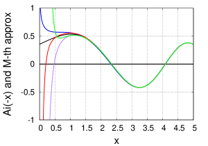
Figure 1: $Ai(-x)$ (black) and its asymptotic expansion to zero (blue), first (red), second (purple), and third (green) orders.

A simple example is provided by the Airy function of negative argument. In Fig 1, we plot this exactly and using its asymptotic expansion of ever increasing order:

$$Ai(-x)=\frac{1}{{\sqrt{\pi}}x^{1/4}}\Im\{e^{i(z+\pi/4}\,w(z)\}$$ (4)

where $z=2x^{3/2}/3$ and

$$w(z)=\sum_{j=0}^{\infty}w_{j}(z)=1-\frac{5i}{72z}-\frac{385}{10368z^{2}}+..,$$ (5)

where $w_{0}=1$, and

$$w_{j+1}=-\frac{i}{2z}\left(j+\frac{5}{36(j+1)}\right)\ w_{j}.$$ (6)

From Fig. 1 we see that, for $x$ sufficiently large (here about 1.5), the asymptotic expansion is extremely accurate. On the other hand, for $x$ sufficiently small, succesive orders worsen the approximation, and zero-order is least bad. Moreover, inbetween, such as at $x=1$, addition of orders at first improves the result and then worsens it.

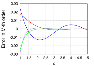
Figure 2: Errors at each order, labelling same as Fig 1.

In Fig. 2, we plot the errors of the successive asymptotic approximatons. First note that the scale is 30 times smaller than Fig. 1, and we have begun at $x=1$. We see that even at $x=2$, the asymptotic behavior has kicked in, and incredibly tiny errors are made even for $M=2$. To be certain that this is truely an asymptotic expansion, even though the terms in Eq. 5 appear to be getting smaller, Eq. 5 shows that as $j\to\infty$, $w_{j}\approx j!/z^{j}$ which diverges for any value of $z$.

So, suppose we wish to approximate $Ai(-x)$ for all $x$ starting at some finite value, such as $x=1$. We define $M_{o}(x)$ as the value of $M$ with the least error, which we refer to as the optimal truncation. Then, if we want a ‘best’ approximation to our function by truncating our asymptotic expansion, we truncate at $M_{o}(1)$. We know that as $x$ increases (at least in the asymptotic regime), the error of this truncated expansion will reduce. Thus we expect our maximum error to be at our lowest $x$, and this truncation will minimize our worst error. In the top half of Table 1, we illustrate this with several orders and several values of $x$.

Order	0	1	2	3	$M_{o}$
$x$	Errors
0.5	0.0964	-0.0069	-0.3893	0.1192	1
1.0	0.0247	0.0177	-0.0291	-0.0248	1
1.5	-0.0029	0.0094	-0.0020	-0.0042	2
2.0	-0.0123	0.0033	0.0010	-0.0002	3
$x$	Additions
0.5	0.5721	-0.1033	-0.3824	0.5085	1
1.0	0.5602	-0.0070	-0.0468	0.0043	1
1.5	0.4614	0.0123	-0.0114	-0.0022	2
2.0	0.2151	0.0156	-0.0022	-0.0012	3

Table 1: Errors in asymptotic expansion of $Ai(-x)$, and contributions added at each order.

But hold on. We have surely cheated here, because we used our knowledge of the error to choose where to truncate, which required knowing the function in the first place! However, a simple heuristic that usually works is to simply look at the magnitude of the terms that are being added in each increase in order. These will typically reduce at first, and then eventually increase. The pragmatic optimal truncation procedure is to simply stop when the next addition is larger in magnitude than the previous one. We see in Table 1 that this indeed corresponds to optimal truncation.

Of greater interest for our purposes will be the asymptotic expansion for the zeroes of $Ai(-x)$, defined by

$$Ai(-a_{j})=0,~{}~{}~{}~{}~{}j=1,2,3...$$ (7)

in order of increasing magnitude. Later, we will show that these are the eigenvalues of a potential. Each order of truncation of the expansion of $Ai(-x)$ in Eq. 4 implies an asymptotic expansion of $a_{j}$ to the same order, yielding

$$a_{j}=y_{j}^{2/3}\sum_{n=0}^{M}\frac{T_{n}}{y_{j}^{2n}},~{}~{}~{}~{}y_{j}=\frac{3\pi}{2}(j-1/4)$$ (8)

where the $T_{n}$ are found and listed in B (appendix B), the first few being $1,5/48,-5/35,...$. Because the lowest zero is about 2.34, the asymptotic behavior already dominates for every zero.

So far we have covered basics in most methods books, such as ArfkenArfken (1985). But now we approach this from a more modern viewpoint, which holds that often, with the right procedure, much more useful information can be extracted from such an expansion, especially in cases that occur in physical problems, i.e., functions that are solutions to relatively simple differential equationsBerry and Howls (1993). These methods might generically be called hyperasymptoticsBerry and Howls (1990); Costin (2008), and often begin with the ‘asymptotics of the asymptotics’, i.e., asking what is the behavior of $c_{n}$ for large $n$ in Eq. 1. Knowing this, one can use a variety of techniques to approximate the rest of the sum to infinity, and extract features that are entirely missed in the definition given above. However, to take advantage of such techniques, one must be able to write the expansion to arbitrary order, and then deduce its behavior.

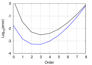
Figure 3: Expansion to many orders of $a_{1}$, the lowest zero of $Ai(-x)$: the additions (black) and errors (blue).

In Fig. 1, we see the first two zeroes, at about 2.34 and 4.09. In Fig. 3, we plot both the magnitude of the correction and the magnitude of the error, on a log (base 10) scale, as a function of the order of the approximation, $M$, in Eq. 8. We see the generic nature of the asymptotic expansion. For small $M$, the additions are quite large. To zero order, the error is of order 0.02. As more terms are added, the magnitude of the additions becomes smaller, as does the error. But at $M=4$, the magnitude of the correction is larger than that of $M=3$, so 3 is the optimal truncation point. We see that indeed the error also begins to grow. For large $M$, the additions become so big that they dominate the error, so the two curves merge. Thus, with simple optimal truncation, our best possible estimate for the lowest zero is with $M=3$.

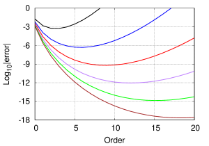
Figure 4: Errors of Fig. 3, but now for first 6 zeroes, the first being black, the 6th being brown.

In Fig. 4, we show what happens for higher zeroes. Now the blue curve shows the magnitude of the error for the second zero. Because it is at a higher value, the optimal truncation occurs at larger $M$, here about 6. In fact, the analysis of B shows $M_{o}(n)\to{\lfloor}\pi*n{\rfloor}$ for the $n$-th zero as $n\to\infty$. The brown curve is for the sixth level, where the lowest error is at $M$ about 18, and is of order $10^{-18}$. This demonstrates the insane levels of accuracy that can be achieved with very elementary means using asymptotic expansions.

Even the lowest order asymptotic expansion is often rather accurate, once the asymptotic parameter does not come close to 0. To write an approximate formula and apply it to all zeroes, one should optimally truncate for the lowest level: All higher levels will then have lower errors (no lines cross in Fig. 4). For any level above the lowest, much greater accuracy can be achieved by optimal truncation for that level (at a much higher order), but including those higher orders would be disastrous for the approximation of the lower levels. For example, for the 6th level, truncation at 18th order yields errors of order $10^{-18}$, but errors of order $10^{-14}$ for the fifth level, $10^{-10}$ for the 4th, and errors greater than a Hartree for the lowest two levels. To get the lowest error for every level with a given truncation, Fig. 4 requires truncation at 3rd order.

2.2 Notation and potentials

We choose units with $m=\hbar=1$, so the 1d Schrödinger equation is

$$\left\{-\frac{1}{2}\frac{d^{2}}{dx^{2}}+v(x)\right\}\phi_{j}(x)=\epsilon_{j}\,\phi_{j}(x)$$ (9)

where $j=1,2,..M$, if only $M$ states are bound. We will consider a variety of shapes of potential and boundary conditions. A hard-wall boundary condition is one where the wavefunction vanishes identically, and nothing exists beyond the wall. An asymptotically bound potential is one where the potential diverges as $x\to\infty$, so that the system has only discrete states. Hard walls are a subset of these. Finally, there is the situation that is closer to realistic, where the potential is asymptotically free, i.e., tends to a finite constant. We assume $v(x)$ has a minimum which we choose to be at the origin, and set the constant to make $v(0)=0$. Thus such potentials tend to $D$ as $x\to\infty$, where $D$ is the well-depth.

Specific examples in this paper include the particle in a box, where $v=0$ between hard walls at $x=\pm L/2$, with eigenvalues

$$\epsilon^{\rm PIB}_{j}=\frac{\pi^{2}\,j^{2}}{2L^{2}}~{}~{}~{}~{}~{}(PIB).$$ (10)

and the harmonic oscillator $\omega^{2}x^{2}/2$,

$$\epsilon_{j}=\omega(j-\frac{1}{2})~{}~{}~{}~{}~{}~{}(HO).$$ (11)

(The unfamiliar minus sign is because the index $j$ begins at 1.) Another analytically solvable case is the Poschl-Teller (PT) well of depth $D$

$$v(x)=D-D/\cosh^{2}(x),~{}~{}\epsilon_{j}=D-(\alpha_{e}+\frac{1}{2}-j)^{2}/2~{}~{}~{}(PT),$$ (12)

where $\alpha_{e}={\sqrt{2D+1/4}}$ and $j<\alpha_{e}+1/2$. Our last (and most interesting) example is the linear well $F|x|$, with $F$ a positive constant whose eigenvalues are

$$\epsilon_{j}=\left(\frac{F^{2}}{2}\right)^{1/3}d_{j}~{}~{}~{}~{}(LW),$$ (13)

where $d_{2j+1}$ is the $j$-th zero of $Ai^{\prime}(-x)$ and $d_{2j}$ is the $j$-th zero of $Ai(-x)$.

For a symmetric potential $v(x)$, one can always place a hard wall at the origin. Then the states of odd parity (even number with our indexing) become the only eigenstates. We call these half wells. For example, for the linear half-well with $F={\sqrt{2}}$, only the even levels survive, and are given precisely by the zeroes of $Ai(-x)$ shown in Fig. 1, i.e., $d_{2j}=a_{j}$ of Eq. 8.

2.3 Non-interacting (Kohn-Sham) fermions

In text books, one usually solves these 1d problems for individual eigenstates. But we consider these as KS potentials of some many-body problem, presumably with some approximate XC functional. As such, we occupy the lowest $N$ levels. If we keep all spins the same, the total energy is then

$$E_{N}=\sum_{j=1}^{N}\epsilon_{j}.$$ (14)

For our simple examples,

$$E_{N} = \frac{\pi^{2}}{6L^{2}}\left(N^{3}+\frac{3}{2}N^{2}+\frac{1}{2}N\right)~{}~{}(PIB)$$ (15)

$$= \omega\frac{N^{2}}{2}~{}~{}~{}~{}(HO)$$

$$= \frac{\alpha_{e}}{2}N^{2}-\frac{N^{3}}{6}-\frac{N}{12}~{}~{}~{}(PT)$$

$$= \sum_{j=1}^{N}a_{j}~{}~{}~{}(LHW).$$

In the last case, there is no simple exact closed form.

The central problem of orbital-free density functional theoryThomas (1927); Fermi (1928); March (1957); Teller (1962); Levy et al. (1984); Parr and Yang (1989); Dreizler and Gross (1990); Wang and Carter (2000) is to find sufficiently accurate approximations for $T_{\scriptscriptstyle\rm S}[n]$, the kinetic energy of non-interacting electrons as a functional of their single particle density, $n({\bf r})$. Functional differentiation and insertion into an Euler equation yields an equation to be solved directly for the density, avoiding the need to solve the KS equations. Here, the required level of accuracy is substantially higher than for XC, as the kinetic energy is comparable to the entire KS energy. Moreover, since the density of a given problem will be found by minimizing the energy with the approximate $T_{\scriptscriptstyle\rm S}[n]$, the functional derivative must also be sufficiently so that the approximate density also does not produce an unacceptable errorKim et al. (2013).

In fact, the original Thomas-Fermi (TF) theoryThomas (1927); Fermi (1928) has precisely this form for the kinetic energy, but it is not very accurate, its underlying density has many peculiarities, and it does not even bind atoms in moleculesTeller (1962). The form of the TF kinetic energy for spin-unpolarized electrons in 3d is simply:

$$T_{\scriptscriptstyle\rm S}^{\rm TF}[n]=\frac{3(3\pi^{2})^{2/3}}{10}\int d^{3}r\,n^{5/3}({\bf r}).~{}~{}~{}({\rm 3D,~{}unpol.})$$ (16)

We will call electrons in a KS potential NIFs, meaning non-interacting fermions. The effect of the Pauli principle is simply to make them occupy the lowest $N$ orbitals. Moreover, to avoid keeping track of endless factors of 2Oliver and Perdew (1979), we simply choose them all to have the same spin. For such spin-polarized NIFS in 1D, the analog of the above is

$$T^{\rm TF}[n]=\frac{\pi^{2}}{6}\int_{\infty}^{\infty}dx\,n^{3}(x).~{}~{}~{}({\rm 1D,~{}pol.})$$ (17)

This is of course the local density approximation for the kinetic energy, and is exact for a fully polarized uniform electron gas. (As densities scale with inverse volume, and the kinetic energy operator is a square gradient, in $d$ dimensions the local density approximation to $T_{\scriptscriptstyle\rm S}$ always has power $n^{(d+2)/d}$, and its prefactor is determined by the uniform gas or the large $N$ limit of any system.)

Thus if one could achieve very high accuracy in an approximate $T_{\scriptscriptstyle\rm S}$ without incurring much computational cost beyond TF, orbital-free DFT could make solving the KS equations obsoleteWang and Carter (2000), and reduce the cost of DFT calculations to that of solving Poisson’s equation. From a regular quantum viewpoint, this is all a very elaborate approach to approximating the sum in Eq. 14.

2.4 Semiclassical approximations

Semiclassical approximations are ubiquitous in physics and chemistry, but are rarely used directly in electronic structure calculations at presentHeller (2018). All such expansions involve powers of $\hbar$ that become relatively accurate in the small $\hbar$ limit. Our interest will be in finding eigenstates of the Schrödinger equation, specifically in one dimension. In this case, the WKB approximationWentzel (1926); Kramers (1926); Brillouin (1926); Dunham (1932) is well-known and appears in many introductory text on quantum mechanicsGriffiths (2005). The WKB formula for eigenvalues is the implicit formula

$${\cal A}(\epsilon)=2\pi(j-\beta/4),~{}~{}~{}~{}~{}j=1,2,...,$$ (18)

where ${\cal A}$ is the classical action at energy $\epsilon$ over a complete closed orbit and $\beta$ is the Maslov indexMaslov and Fedoriuk (2001). The Maslov index distinguishes between hard wall reflections and true turning points, i.e., those where the slope of the potential is finite. There is no contribution for a hard wall, but for each true turning point, $\beta$ increases by 1. For our 1d examples, each full orbit yields a contribution equal to double a transit from left to right. Thus we write

$$I^{\text{WKB}}(\epsilon)=\int_{-\infty}^{\infty}dx\,p(x,\epsilon)=j-\nu,$$ (19)

where $p=\Re{\sqrt{2(\epsilon-v(x))}}$ is the classical momentum at energy $\epsilon$ in the well, and $\nu=0$ if there are only hard walls, and increases by $1/4$ for each true turning point.

We can apply the WKB approximation to each of our wells. For the PIB, $v=0$, $p={\sqrt{2\epsilon}}$ and $I^{\text{WKB}}=Lp$, yielding the exact answer as $\nu=0$. Similarly, for the HO, and $I^{\text{WKB}}=\epsilon/\omega$, again yielding the exact answer, as $\mu=1/2$. The first can be attributed to the equivalence of semiclassical and exact quantum motion for a constant potential, the second to the exactness of semiclassical results in harmonic potentials. For the PT well,

$$I^{\text{WKB}}(\epsilon)={\sqrt{2D}}-{\sqrt{2D-\epsilon}}~{}~{}~{}~{}(PT),$$ (20)

which recovers the dominant semiclassical approximation, using $\nu=1/2$:

$$\epsilon^{\text{WKB}}(x)={\sqrt{2D}}x-x^{2}/2~{}~{}~{}~{}(PT).$$ (21)

Finally, for the linear half-well, with $\nu=1/4$:

$$I^{\text{WKB}}(\epsilon)=\frac{2}{3\pi}\epsilon^{3/2},~{}~{}~{}\epsilon^{\text{WKB}}(x)=\left(\frac{3\pi x}{2}\right)^{2/3}.$$ (22)

In fact, for $F={\sqrt{2}}$, these are precisely the zeroes of the leading order expansion of $Ai(-x)$ of Sec. 2.1. For the linear half-well, the exact expression for $I$ is

$$I(\epsilon)=\frac{z+\Im{(\log w(z))}}{\pi},~{}~{}~{}~{}z=\frac{2}{3}\epsilon^{3/2}~{}~{}~{}(LHW),$$ (23)

where

$$w(z(x))={\sqrt{\pi}}x^{1/4}\,e^{-i(z+\pi/4)}\left(Bi(x)+iAi(-x)\right),$$ (24)

and $Bi(x)$ is the other independent solution of the Airy equationAbramowitz and Stegun (1965); DLMF . For every well in Sec. 2.2,

$$\epsilon_{j}\to\epsilon^{\text{WKB}}(j-\nu),~{}~{}~{}~{}~{}j\to\infty.$$ (25)

But the WKB approximation is just the first term in a delicate asymptotic expansion in $\hbar$, as shown by DunhamDunham (1932). We can define an expansion in powers of $\hbar$, here represented by a dimensionless parameter $\eta$, via

$$I_{\eta}(\epsilon)=\sum_{k=0}^{\infty}\eta^{2k}\,I^{(2k)}(\epsilon),$$ (26)

where $I^{\text{WKB}}$ is just the leading term. Then

$$I_{\eta}(\epsilon)=\eta(j-\nu),$$ (27)

determines the eigenvalues implicitly, which can be inverted power by power to yield an expansion for the energy levels which becomes more accurate as $j$ increases. This expansion is well-knownBender and Orszag (1978), but is subtle for systems with turning points. The naive corrections formally diverge at the turning points, but these divergences are exactly cancelled by other terms in the wavefunction, yielding finite contributions in every order. This is the semiclassical expansion we are interested in, but we wish to find sums over levels, not individual eigenenergies.

Back in the 1950’s and 1960’s, there was considerable activity attempting to use semiclassical approximations to do electronic structure calculations, especially by the Miller groupMiller (1968a, b). In fact, Kohn and Sham developed a remarkably insightful approachKohn and Sham (1965b) just months before their most popular paperKohn and Sham (1965a), whose ultimate success for numerical computation overwhelmed interest in semiclassical approaches. There was much interest in semiclassical methods for more than one dimension in the area of quantum chaosBerry (1983).

One can also deduce, e.g., approximate wavefunctions (see Sec. 2.8 below) in the WKB expansionGriffiths (2005). Using WKB wavefunctions to find approximate energies, e.g., by evaluating the Hamiltonian on them, yields different resultsLindblom and Robiscoe (1991) than those for the eigenvalues, Eq. 18. All semiclassical methodsM.V. Berry (1972) require extreme care in defining precisely the nature of the expansion and which quantities should be held fixed.

2.5 Semiclassical limit

We next consider specifically the semiclassical limit for the sum of the energies. In this case, one simply integrates the WKB energies over the required number of levels. For almost any potential, it can be shown numerous ways thatMarch and Plaskett (1956)

$$E_{N}\approx\int_{0}^{N}dx\,\epsilon^{\text{WKB}}(x)\approx E^{\rm TF}_{N},~{}~{}~{}~{}\hbar\to 0,$$ (28)

and none of the details of the corrections matter. The TF approximation can be treated as a functional of either the density or the potential (see Sec 2.7 below) and the results are the same. Alternatively, it is a straightforward matter to extract the kinetic contribution aloneMarch and Plaskett (1956) and find the local density approximation to the kinetic energy. Thus, the local approximation (here TF) becomes relatively exact for all problems in this semiclassical limit. This is a simple case of the much harder proof by Lieb and Simon of the same statement for all Coulomb-interacting matterLieb and Simon (1977). In the language of Sec 2.1, the TF theory yields the dominant contribution in an asymptotic series for all matter, which implies that its relative error vanishes in the limit, Eq. 2.

2.6 Gradient expansion in DFT

We focus here on the non-interacting kinetic energy, whose gradient expansion was performed by KirzhnitsKirzhnits (1957), for a slowly-varying gas, using the Wigner-Kirkwood expansionWigner (1932); Kirkwood (1933). Ideas of gradient expansions permeate the HKHohenberg and Kohn (1964) and KS papersKohn and Sham (1965a) that created modern DFT, for both the full functional and its XC contribution. The first generalized gradient expansion for correlation was from Ma and BrucknerMa and Brueckner (1968), from which many modern GGA’s are descended.

Here we consider only the non-interating kinetic energy in one dimension. In that case, Samaj and Percus did a thorough jobSamaj and Percus (1999), showing how to generate the expansion to arbitrary order. We focus on several key points. First, they expand both the density and the kinetic energy density as functionals of the potential. (This is, after all, how quantum mechanics normally works.) Given a potential, the expansion for the density is

$$n(x)=\frac{k_{\scriptscriptstyle\rm F}(x)}{\pi}\sum_{j=0}^{\infty}\frac{a_{j}(x)}{k_{\scriptscriptstyle\rm F}^{2j}(x)\beta_{j}},$$ (29)

where $\beta_{j}=1-2j$, $k_{F}={\sqrt{2(\mu-v(x))}}$ and $\mu$ is determined by normalization. The analogous formula for a kinetic energy density $t(x)$ is found by multiplying by $k_{F}^{2}(x)/2$ and replacing $\beta_{j}$ by $\beta_{j+1}$, where $t(x)$ is a function whose integral yields $T$. The coefficients in the expansion areSamaj and Percus (1999)

$$a_{0}=1,~{}~{}~{}a_{1}=0,~{}~{}~{}a_{2}=({{k_{F}}^{\prime}}^{2}+k_{F}k_{F}^{\prime\prime})/4,...$$ (30)

Inserting Eq. 29 into $t(x)$, and expanding in small gradients, yields:

$$T^{\rm GEA}[n]=\frac{\pi^{2}}{6}\int dx\ n^{3}(x)-\frac{1}{24}\int dx\left(\frac{dn}{dx}\right)^{2}+..$$ (31)

This is the exact analog of the usual expansion in 3DDreizler and Gross (1990), except this is the spin-polarized form, and the coefficient of the von Weisacker contribution is $1/9$ in 3D but $-1/3$ in 1D. The gradient expansion is known to 6-th order in 3DMurphy (1981) and has been numerically validated under conditions where gradient expansions applyZ.Yan and Ziesche (1997). It has also been noticed that, for non-analytic potentials, evaluation of the higher-order terms depends sensitively on the boundary conditionsJ.P. Perdew and Pathak (1986).

2.7 Potential functionals versus density functionals

The creation of modern DFT and the KS equations has clearly been very successful. However, standard approaches to quantum mechanics yield algorithms that predict, for example, the energy as a functional of a given potential, $v(x)$ here. In the context of KS-DFT, Yang, Ayers, and WuYang et al. (2004) first clearly showed the relation between potential functionals and density functionals. But semiclassical approximations yield results for a given potential, not density. Thus Cangi et alCangi et al. (2011, 2013); Cangi and Pribram-Jones (2015) revisited the entire framework of density functional theory, from the HK viewpoint, and showed that a logical alternative was to create a potential functional that also satisfied a minimum principle, namely

$$F_{v}=F[n_{v}],$$ (32)

where $F[n]$ is the universal part of the energy functional and $n_{v}({\bf r})$ is the ground-state density of potential $v({\bf r})$. Then

$$E_{0}=\min_{v^{\prime}}\left\{F_{v^{\prime}}+\int\,v\,n_{v^{\prime}}\right\},$$ (33)

yields the exact ground-state energy and $v=v^{\prime}$ at the minimumCangi et al. (2013). Given an expression for $n_{v}$, various strategies can be used to construct a corresponding $F_{v}$ and so the entire energy can be found. In the specific case of TF theory, Eq. 17 yields exactly the same results for any system whether expressed as a density functional or a potential functional. More sophistacted approximations for the density including higher-order expansions in $\hbar$ (see next section) are typically not designed to be variationalGross and Proetto (2009), and minimization might worsen results. Such minimizations are not needed if direct application to the external potenial already yields highly accurate resultsCangi et al. (2010).

2.8 Uniform approximations for the density

To find semiclassical expansions for the density as a functional of the potential, one can start from WKB wavefunctions. With hard walls, the wavefunctions are simple

$$\phi_{j}(x)\approx\sqrt{\frac{2\omega_{j}}{p_{j}(x)}}\sin{\theta_{j}(x)}\,,$$ (34)

where $p_{j}(x)$ is the classical momentum in the $j$-th WKB eigenstate, $\omega_{j}$ is the frequency of its orbit, and $\theta_{j}(x)$ is the phase accumulated from the left wallElliott et al. (2008). Using a variation on the standard Euler-Maclaurin formula (Eq. 43 below) in asymptotic form, this yields a uniform approximation to the density. For any value of $x$, WKB provides the dominant contribution as $\hbar\to 0$, and its leading corrections provide the next order in the asymptotic series. Early on, it was shown how to extract an accurate approximation to both the density and the kinetic energy density with hard-wall boundary conditions, by evaluating the next order in the WKB expansion for the wavefunctions, and summing the resultElliott et al. (2008); Cangi et al. (2010). The leading corrections to the kinetic energy density integrated to yield the leading correction to the kinetic energy as an expansion in $\hbar$.

However, the WKB wavefunctions are well-known to diverge at a true turning point. LangerLanger (1937) found a semiclassical wavefunction that remains uniformly accurate through the turning point, by replacing $\sin\theta_{j}$ in Eq. 34 with

$$z_{j}^{1/4}(x)\,Ai\left[-z_{j}(x)\right],$$ (35)

where $z_{j}=\left[3\theta_{j}(x)/2\right]^{2/3}$. Some years laterRibeiro et al. (2015), and with considerable difficultyRibeiro and Burke (2018), it was deduced how to repeat the same procedure for a well with real turning points, creating a uniform approximation for the density in a well with turning points, i.e., one whose error, relative to the local approximation, vanishes for all $x$ as $\hbar$ vanishes. Note that the expansion in $\hbar$ is in different orders depending on how close $x$ is to the turning point.

The resulting approximations are exceedingly accurate for both the density and the kinetic energy density pointwise, but surprisingly do not yield more accurate energiesRibeiro and Burke (2017). When analyzed, it was found that the expansion in wavefunctions yields energetic corrections of order $\hbar^{1/3}$, but the leading corrections are of order $\hbar$Ribeiro and Burke (2017). This was explained by showing that the coefficient of $\hbar^{1/3}$ vanishes identically! Thus, this expansion would have to be continued to two more orders to yield the leading correction to the energy, which might take generations to derive. Instead, analysis of the simple potentialsRibeiro and Burke (2017) used to test the uniform appoximations showed that direct sums over eigenvalues can yield the leading corrections to sums over $N$ occupied orbitals, bypassing (for now) the density and any other real-space quantity entirely.

3 Theory

3.1 Summation formulas

We begin our theoretical development with an unusual form of the Euler-Maclarin formula from HuaHua (2012)

$$\sum_{a\leq j\leq b}f(j)=\int_{a}^{b}dx\left(f(x)+P_{1}(x)f^{\prime}(x)\right)-\left[P_{1}(x)f(x)\right]_{a}^{b}$$ (36)

where $a,b$ are real numbers, $f^{\prime}(x)=df/dx$ must be continuous, and $P_{1}(x)$ is the first periodized Bernouilli polynomialDLMF . The periodized Bernouilli polynomials are

$$P_{k}(x)=B_{k}(x-{\lfloor}x{\rfloor}),$$ (37)

where $B_{k}(x)$ is a Bernouilli polynomial, and where ${\lfloor}x{\rfloor}$ is the integer part of $x$. The Bernouilli polynomials, of order $k$, satisfy many simple conditions, with the lowest few being

$$B_{0}(x)=1,~{}~{}~{}B_{1}(x)=x-\frac{1}{2},~{}~{}~{}B_{2}(x)=x^{2}-x+\frac{1}{6}.$$ (38)

The famous Bernouilli numbers are then

$$B_{k}=B_{k}(1),$$ (39)

which vanish for all odd $k$, except $B_{1}=1/2$. Eq. 36 is an unusual form because $a$ and $b$ are continuous.

We next perform the standard trick of repeated integration by parts, leading to

$$\sum_{a\leq j\leq b}f(j)=\sum_{k=0}^{p}D_{k}+R_{p},$$ (40)

where the end-point contributions are

$$D_{k}=\frac{(-1)^{k}}{k!}\left[P_{k}(x)f^{(k-1)}(x)\right]_{a}^{b},$$ (41)

and the remainder is

$$R_{p}=\frac{(-1)^{p+1}}{p!}\int_{a}^{b}dx\,P_{p}(x)\,f^{(p)}(x).$$ (42)

Eq. 40 is true for any $p\geq 1$, so long as the $p$-th derivative of $f(x)$ is continuous. Here, the term $f^{(-1)}(x)$ is simply the antiderivative, so the integral is $D_{0}$. The $p=1$ case is Eq. 36. We call Eq. 40 the extended Euler-Maclaurin form, and we use several variations in what follows.

We note some remarkable features of Eq. 40. First, any sufficiently smooth function of $x$ that matches $f_{j}$ at the integers yields exactly the same sum, so that all differences in the integral on the right must be cancelled by the other terms. Thus, there are many allowed choices for $f(x)$ that yield the exact sum. Adding any sufficiently smooth $g(x)\sin(\pi x)$ to an acceptable $f$ does not change the sum. Next, we note that for any range of $a$ and $b$ between integers, the sum does not change but the integral does, so again such changes must be absorbed by the remaining terms. Lastly, we note that the formula is exact for every $p$. Choosing a low $p$ requires less derivatives, but often the remainder term is more difficult to evaluate.

Of course, there are many different ways to write this formula that are useful in different contexts. The special case $a=1_{-}$ and $b=N_{+}$ recovers the commonly given form of Euler-Maclaurin,

$$\sum_{j=1}^{N}f_{j} = \int_{1}^{N}dx\,f(x)+\frac{f(N)+f(1)}{2}+R_{p}[f]$$ (43)

$$+ \sum_{k=1}^{{{\lfloor}p/2{\rfloor}}}\frac{B_{2k}}{(2k)!}\left(f^{(2k-1)}(N)-f^{(2k-1)}(1)\right),$$

where the remainder term is the same as above. The plus sign in the second term on the right occurs because of the discontinuity in $P_{1}(x)$ across an integer, and the vanishing of even derivatives is because all odd Bernouilli numbers are zero, except $B_{1}$. This form is perhaps most familar when approximating an integral by a sum, but we never use it here.

Next, consider the special case $0<a<1$ and $b=N+a$. Then the sum becomes specifically that of the first $N$ terms:

$$S_{N}=\sum_{j=1}^{N}f(j),$$ (44)

while the end contributions simplify to

$$D_{k}(a)=\frac{(-1)^{k}}{k!}B_{k}(a)\left[f^{(k-1)}(x)\right]_{a}^{N+a}.$$ (45)

We will have use for two special cases. The first is $a=1/2$, and sinceDLMF

$$B_{k}(1/2)=-(1-2^{n-1})B_{k},$$ (46)

then only even terms contribute to the end-points. The other case we will use is the limit as $a\to 1$, so that $B_{k}(a)=B_{k}$, and

$$D_{k}(1)=\frac{(-1)^{k}}{k!}B_{k}\,\left[f^{(k-1)}(x)\right]_{1}^{N+1}$$ (47)

no longer vanishes for $k=1$. Both these special cases will be of value: The first yields some of the key the results of A, the second of B.

3.2 Sums of eigenvalues

We first use Eq. 36 to derive a general exact formula for the sum of $N$ energy levels in terms of $\epsilon(x)$. From Sec 2.4, we know $\epsilon_{j}=\epsilon(j-\nu)$. Using this, we find for the sum of the first $N$ energies:

$$E_{N}=\sum_{j=1}^{p}D_{k}(a)+R_{p}(a),$$ (48)

where

$$D_{k}(a)=\frac{(-1)^{k}}{k!}B_{k}(a)\left[\epsilon^{(k-1)}(x)\right]_{\alpha}^{N+\alpha},$$ (49)

and

$$R_{p}(a)=\frac{(-1)^{p+1}}{p!}\int_{\alpha}^{N+\alpha}dx\,P_{p}(x+\nu)\,\epsilon^{(p)}(x),$$ (50)

with $\alpha=a-\nu$. In the special case $a=\nu$, all integrals and evaluations run from 0 to $N$. Finally, for the standard case of two real turning points, insert $\nu=1/2$ in both $D_{k}(\nu)$ and $R_{p}(\nu)$ to yield

$$E_{N}=\int_{0}^{N}dx\,\epsilon(x)+\sum_{k=1}^{p}D_{k}(\frac{1}{2})+R_{p}(\frac{1}{2}).$$ (51)

For the choice $p=1$, because $B_{1}(1/2)=0$ the end-term vanishes, yielding the elegant result

$$E_{N}^{2TP}=\int_{0}^{N}dx\,\left(\epsilon(x)+{\langle}x{\rangle}\epsilon^{\prime}(x)\right)~{}~{}~{}(\nu=\frac{1}{2},p=1)$$ (52)

where ${\langle}x{\rangle}=P_{1}(x+1/2)$, and $2TP$ denotes two turning points. This is recognizable as Eq. 14 of A, but was derived here by more elementary means.

The analysis of A is confined to $\nu=1/2$ and $p=1$. The current formulas apply to all possible potentials, i.e., any Maslov index, and allow higher choices of $p$. For example, the $p=1$ result for arbitrary $\nu$ yields

$$E_{N}=E_{N}^{2TP}+(\frac{1}{2}-\nu)\left[\epsilon(x)\right]_{0}^{N},~{}~{}~{}(p=1)$$ (53)

i.e., there is a simple correction whenever $\nu$ differs from 1/2. It is straightforward to check that Eq. 53 produces the exact sum when used correctly. For example, for a half-harmonic oscillator, $\nu=1/4$ and $\epsilon(x)=2\omega x$. In this case, the 2TP contribution is easy to calculate as the second term vanishes, due to the constancy of $\epsilon^{\prime}$ and the periodicity of ${\langle}x{\rangle}$, yielding $\omega N^{2}$. But there is also a finite addition of $\epsilon(N)/4$ to produce the exact $E_{N}=\omega N(N+1/2)$. Similar corrections are also needed to recover the exact sum for the particle in a box. This illustrates the significance of the correct Maslov index in all such calculations.

3.3 Leading correction to local approximation

In this section, we use Eq. 40 to examine just the leading correction to the local approximation. Because classical action is a monotonically increasing function of $\epsilon$ as one climbs up a well, then $\epsilon(x)$ also grows monotonically, so its integral grows even more rapidly. On the other hand, its derivative will be less rapidly growing, and the periodic term ${\langle}x{\rangle}$ averages to zero with a constant function. Thus this term is smaller than the dominant term.

Expanding $I$ in even powers of $\eta$ as in Eq. 27, we find two leading corrections to the local approximation to second order:

$$\Delta E^{(2)}_{N}=\int_{0}^{N}dx\,\left(\epsilon^{(2)}(x)+{\langle}x{\rangle}\frac{d\epsilon^{(0)}}{dx}\right).$$ (54)

Thus there are two corrections: Those due to the next order in the WKB expansion inside the dominant integral while others are the error made in approximating the sum over WKB eigenvalues by an integral. In the case of extended systems where there are no turning points, i.e., slowlying varying densities, the spacing between levels goes to zero in the thermodynamic limit, and the latter correction vanishes. Thus the gradient expansion of Sec. 2.6 misses such terms completely.

In principle, Eq. 53 also applies to the linear well, but its expansion is more difficult than the previous case. In particular, the asymptotic expansion diverges at $x=0$, the start of our integral, making it impossible to work with. We thus use a different version, as developed in B.

3.4 Hyperasymptotics

We now turn to the work of Ref B. We see immediately that Eq. 52 is not useful for asymptotic expansions in powers of $\hbar$, as it includes energies down to zero, where asymptotic expansions like that of Eq. 1 diverge. In fact, we use Eq. 47, in which both $a$ and $b$ have been maximized, for a given sum from 1 to $N$. This idea already appeared in the contour chosen in Ref Kohn and Sham (1965b), which circles a pole in the Green’s function at $\epsilon_{N+1}$. Thus we choose our second variation to explore asymptotic expansions:

$$D_{k}(1)=\frac{(-1)^{k}}{k!}B_{k}\left[\epsilon^{(k-1)}(x)\right]_{{\bar{\nu}}}^{N+{{\bar{\nu}}}},$$ (55)

and

$$R_{p}(1)=\frac{(-1)^{p+1}}{p!}\int_{{\bar{\nu}}}^{N+{\bar{\nu}}}dx\,P_{p}(x+\nu)\,\epsilon^{(p)}(x),$$ (56)

where ${\bar{\nu}}=1-\nu$. The first three $D$’s are:

$$\left[E(x)\right]_{\bar{\nu}}^{N+{\bar{\nu}}}-\frac{1}{2}\left[\epsilon(x)\right]_{\bar{\nu}}^{N+{\bar{\nu}}}+\frac{1}{12}\left[\epsilon^{\prime}(x)\right]_{\bar{\nu}}^{N+{\bar{\nu}}},$$ (57)

where $E(x)$ is the antiderivative of $\epsilon(x)$. These forms apply to all wells for any $p>0$, but have the advantage of being evaluated at the largest possible energies.

It is trivial to check that these forms yield both the exact results for all the simple potentials we have encountered so far, for any choice of $p$. They also recover the leading correction to the semiclassical expansion for the PT well, producing two corrections, one from the 2nd-order WKB, and the other either from $D_{1}$ or $R_{1}$, just as in Eq. 54.

But the real use is in hyperasymptotics, i.e., performing asymptotic expansions to high orders. We apply our formulas to the half linear well, so that $\nu=1/4$ and ${\bar{\nu}}=3/4$. We perform the WKB expansion to find an asymptotic series in even powers of $\eta$ for the energies:

$$\epsilon_{m}(x)=\sum_{p=0}^{m}\epsilon^{(2p)}(x).$$ (58)

Inserting this in the summation formula, we chose $p=m$, which guarantees the remainder term is of order $m+1$ or greater. The $k$-th end-point term contains orders $k-1$ to $m+k-1$ due to the derivatives, but the terms beyond $m$ can be discarded to find the asymptotic approximant of order $m$. We can write the result very simply as:

$$E_{N}\approx\sum_{m=0}^{M}\left(S_{m}(N+{\bar{\nu}})-S_{m}({\bar{\nu}})\right),$$ (59)

where

$$S_{m}(x)=\sum_{k=0}^{m}\frac{B_{2k)}}{(2k)!}\epsilon^{(2(m-k),2k-1)}(x)-\frac{1}{2}\epsilon^{(2m)}(x),$$ (60)

where the first superscript indicates the power of expansion in $\eta$ and the second denotes the number of derivatives taken. This recovers exactly the expansion in Eq. (6.4) of Ref B. The asymptotic expansion is evaluated at $N+1$ rather than at $N$ in the regular EM formula. This confers two distinct advantages: For a given order, our errors are typically much smaller when the index is increased by 1, and secondly, since the order of optimal truncation is ${\lfloor}\pi N{\rfloor}$, by evaluating at $N+1$, three additional orders are added to the optimally truncated series, with their concommitant improvement in accuracy.

We note that one need only evaluate each contribution in Eq. 59 at the upper end. Taking $N=0$ and subtracting then yields $S_{N}$, guaranteeing correctly its vanishing for $N=0$. Thus we have recovered the main one-dimensional result of Ref B without need for (but also missing the elegance of) regularizing sums as $N\to\infty$. Eq. 59 can be applied directly to finite wells, such as PT or the truncated linear half-well of Ref. Berry and Burke (2019).

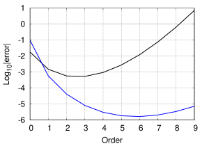
Figure 5: Errors of Fig. 3 (black) and from summation formula, Eq. 66 (blue).

We show some results from the summation formula for the linear half well in Fig. 5 for $N=1$, where $E_{1}=\epsilon_{1}$. The summation formula is less accurate than the original formula for $M=0$, but is much more accurate even for $M=3$ (by two orders of magnitude). More importantly, its optimal truncation is at 6, producing almost 3 orders of magnitude in improvement, i.e., going from milliHartrees to microHartrees errors!

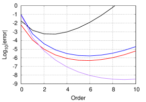
Figure 6: Same as Fig. 5, but adding curves for first excited state (red) and the sum of lowest two energies (purple).

To see that this is due to our evaluation at $N+1$, in Fig. 6 we add in the second eigenvalue and the second sum, $E_{2}=\epsilon_{1}+\epsilon_{2}$. Its error curve is almost identical to that of the summation formula for the first level. Of course, the summation formula for the 2nd level has leaped ahead again, with errors of nanoHartrees at the optimal truncation of $M=9$!

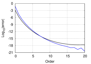
Figure 7: Same as Fig. 5, but for the 6th level and its sum.

Finally, we attempt to show the error in the 6th level in Fig. 7. The black line here is for the error in individual level, and so matches the purple line of Fig. 5. But the blue line is the error in the summation formula, which appears to be least at optimal truncation of about $M=21$, where the error is about 10 zeptoHartrees. (The noise in the curve is caused by numerical imprecision.)

3.5 Alternative summation formula

So far, our analysis has shown that the key formulas of A and B are special cases of the extended Euler-Maclaurin formula, Eq. 40. The formulas of A apply only to two turning points, and cannot be used as a basis for asymptotic expansion, because the energy function must be evaluated at 0. The formulas of B require an infinite set of eigenvalues, but our Eq. 60 allows them to be applied to a finite number. Eq. 60 contains the Maslov index explicitly and has no difficulties at the lower-end, which does not vanish, even in the two turning point case.

But can we find a single formula that covers all cases? The primary aim is to generate an expansion for large $N$, in which one can write exact expressions for the error. For any monontonically increasing function of $x$, as our eigenvalues are defined to be, the large-$N$ limit of the sum is dominated by the integral. The leading correction is always given by the end-point contribution near $x=N$. Thus, choosing our upper end-point as $N+1/2$ always eliminates that contribution, simplifying the result. Equally, we choose $a=1$ always, so that the lower energy, even in the presence of two turning points, does not vanish. This yields the ungainly but practical

$$E_{N}=\int_{a}^{b}dx\epsilon(x)-\sum_{k=1}^{{\lfloor}p/2{\rfloor}}\frac{B_{2k}}{(2k)!}(1-\frac{2}{4^{k}})\,\epsilon^{(2k-1)}(b)+\Delta_{p},$$ (61)

where $b=N+1/2-\nu$, $a=1-\nu$, and $\Delta_{p}$ is of order $\epsilon^{(2p)}(N)$ and is given exactly by

$$\Delta_{p}=-\sum_{k=1}^{p}\frac{B_{k}}{k!}\epsilon^{(k-1)}(a)+R_{p}.$$ (62)

Since the integration interval is no longer an integer, $R_{p}$ does not vanish beyond a maximum $p$ for simple powers. We emphasize that this is an exact formula for all potentials that are sufficiently smooth (the $p$-th derivative must be continuous), and can be applied with any $p\geq 1$, and to any boundary conditions. Curiously, almost the same form (but with $a=1/2$) was used in Eq. 22 of Ref. Cangi et al. (2010) to perform the summation correctly, but without explanation for why it had this form, or the role of the Maslov index.

For the linear half well, Eq. 61 yields the simple closed-form asymptotic expansion

$$E_{N}\approx\sum_{j=0}^{\infty}d_{j}y_{N}^{5/3-2j},~{}~{}~{}~{}y_{N}=\frac{3\pi}{2}\tilde{N},$$ (63)

where $\tilde{N}=N+1/4$, and

$$d_{j}=\frac{2}{3\pi}\frac{T_{j}}{5/3-2j}-\frac{\pi}{16}T_{j-1}(8/3-2j).$$ (64)

This generates exactly the same asymptotic expansion in $N$ as Eq. 6.4 of B, but in a simpler form and with terms that differ only by even powers of $z_{n}$. The first two terms are:

$$E_{N}\approx\left(\frac{3\pi}{2}\right)^{2/3}\left(\frac{3}{5}\tilde{N}^{5/3}-\frac{5+\pi^{2}}{36\pi^{2}\tilde{N}^{1/3}}+...\right).$$ (65)

This is identical to, but simpler than, Eq. (6.4) of B. The GEA of Sec. 2.6 includes only contributions from the integral in Eq. 61. In the 2nd term, GEA does not include the $\pi^{2}$ contribution in the numerator, reducing the overall coefficient by a factor of about 3, and so misses the correct asymptotic expansion.

4 Relation to DFT

4.1 Error in gradient expansion

While these are impressive ways to sum $N$ eigenvalues, what do they mean for DFT calculations? We focus on the relation to orbital-free DFT in one dimension (not a very practical application, admittedly).

We first consider the direct potential functional form of the gradient expansion, given in Eq 29 of Sec 2.6. All terms can be combined to yield the gradient expansion for the total energy. This yields formulas identical to those we find from the WKB expansion inserted into the integral term, $D_{0}$, and totally misses the corrections from the rest of the expansion for any system with discrete levels, as are atoms and molecules. If this term is included, the results are much more accurate (see Table I of A), because the correct asymptotic expansion has been included to the given order. As shown throughout these works, the sums are much more accurate than the original expansion for the individual levels. Without this term, one has only part of the correction, and can make at best crude guesses (possibly using exact conditions) that yield moderate improvements at best over the excellent zero-th order contribution.

In Ref A, the correction was first isolated, but only for $\nu=1/2$. We can now give the corrections in all cases to every order. In Eq. 59, the gradient expansion accounts only for those terms of order $m$ in the WKB expansion that occur with the same order in the summation, i.e., only the $D_{0}$ contribution to the sum. Thus

$$S^{GEA}_{m}(x)=E^{(2m)}(x)-\frac{1}{2}\epsilon^{(2m)}(x).$$ (66)

for $m>0$, and the missing terms are

$$\Delta S^{GEA}_{m}(x)=\sum_{k=1}^{m}\frac{B_{2k)}}{(2k)!}D_{2k-1}\epsilon^{(2(m-k))}(x).$$ (67)

For example, the leading-order missing correction is

$$\Delta S^{GEA}_{1}(x)=\frac{1}{12}\frac{d\epsilon^{(0)}}{dx}.$$ (68)

This is the term that was identified in A. Without it, the 2nd-order gradient expansion approximation was, at best, an erratic correction to the local approximation. Including it gave accuracies about 30 times better than the dominant term. Again, adding the next order led to errors of microHartree order. Our formulae allow one to extract this missing term to any Maslov index, and so allow it to be computed, e.g., for the linear half-well. More importantly, they can be (in principle) applied to all orders (once the WKB expansion has been performed to a similar order).

4.2 Understanding aspects of practical KS-DFT

This 1D world may seem very far from the real world of realistic, practical electronic structure with Coulomb-repelling electrons being Coulomb-attracted to nuclei, but many of the difficulties and problems with practical approximate functionals show up in simpler forms here.

For example, many semilocal functionals perform worst for one particle. We see here that all our results are worst for the lowest level, because the expansion is asymptotic in the particle number, $N$. Hence self-interaction errorPerdew and Zunger (1981) is a chief source of error in semilocal XC calculations.

Semilocal approximations to XC fail when a bond is stretched, often breaking symmetry at a Coulson-Fischer pointCoulson and Fischer (1949). We see here that, as a bond is stretched, there is a critical distance in which the well goes from a single well to two. Beyond that point, one can perform the expansion in the separate wells, but it is a different expansion from the one that applies to a single well. Thus the asymptotic expansion relevant at equilibrium becomes irrelevant (and so highly inaccurate) as the well splits in two. For interacting electrons, this effect is accompanied by a multi-reference character to the interacting wavefunction.

A third insight, not explored here, is the derivative discontinuities in the energies as a function of continuous particle number $N$Perdew et al. (1982); Perdew (1985). The methodology of A demonstrates this explicitly, and the present techniques will be expanded to include this in the future.

4.3 Importance for practical calculations

Insights from studying these one-dimensional situations have already contributed to understanding and creating modern functional approximations. For example, the parameter in B88 exchange GGABecke (1988) was derived in Ref. Elliott and Burke (2009), a mere 21 years after it was first proposed. The derivation yields a value within 10% of the fitted value of B88 (and is less accurate for real systems). One of two crucial conditions in constructing PBEsolPerdew et al. (2008), namely the restoration of the second-order gradient expansion for exchange, came from these insights. In fact, the current work may lead to insight into the second condition, which is the restoration of the LDA surface energy for jellium. Eq. 65 contains a correction missed by the GEA due to the surface of a linear potential, just the kind of correction being extracted from the edge electron gasKohn and Mattsson (1998); Armiento and Mattsson (2005); Lindmaa et al. (2014). Moreover, Ref. Cancio et al. (2018) showed that even the correlation energy of finite systems finally tends to its LDA value (at least for atoms, but logarithmically slowly). Several of these asymptotic conditions for atoms as $N\to\infty$ were built into SCANSun et al. (2015) and other approximate functionalsConstantin et al. (2011a). Finally, we mention that all chemical and materials properties depend on energy differences, not total energies. Ref. Constantin et al. (2011b) showed that, for atoms with certain plausible assumptions, the ionization potential is given exactly by KS-LDA calculations in the asymptotic limit.

It is tantalizing to note that Ref. Elliott and Burke (2009) found that the asymptotic correction to the local density approximation for exchange was almost exactly double that of the gradient expansion. This could only be done by numerical extraction of the coefficient from a sequence of large atom Hartree-Fock calculations. Eq. 65 finds analytically that the correction to the local density approximation for the total energy of the linear half-well is almost exactly triple that of the gradient expansion.

5 Conclusions

I have presented an appropriate mathematical tool for understanding the successes of modern density functional theory and the centrality of the local density approximation. In this framework, the continuum limit achieved as $\hbar\to 0$ in a certain, very well-defined sense is the reason behind the success of semilocal density approximations. This framework unites two (apparently) distinct approaches in previous papers, and generalizes key results from both those works. More importantly, it shows that, at least in principle, DFT approximations need not be of low accuracy. In the simple case studied here, a well-defined correction has been identified that is missing from the starting point of most modern approximate schemes, i.e., the gradient expansion, and its recovery has greatly improved accuracy in model cases. Further work will follow.

This research was supported by NSF (CHE 1856165). Kieron Burke thanks Bob Cave, Attila Cangi, and Raphael Ribeiro for critical readings of the manuscript.

References

- Pribram-Jones et al. (2016) A. Pribram-Jones, P. E. Grabowski, and K. Burke, Phys. Rev. Lett. 116, 233001 (2016), URL http://link.aps.org/doi/10.1103/PhysRevLett.116.233001.
- Kohn and Sham (1965a) W. Kohn and L. J. Sham, Phys. Rev. 140, A1133 (1965a), URL http://link.aps.org/doi/10.1103/PhysRev.140.A1133.
- Eberhart and Clougherty (2004) M. Eberhart and D. Clougherty, Nature Materials 3, 659 (2004).
- Dreizler and Gross (1990) R. M. Dreizler and E. K. U. Gross, Density Functional Theory: An Approach to the Quantum Many-Body Problem (Springer–Verlag, Berlin, 1990), ISBN 0387519939.
- Perdew et al. (1992) J. P. Perdew, J. A. Chevary, S. H. Vosko, K. A. Jackson, M. R. Pederson, D. J. Singh, and C. Fiolhais, Phys. Rev. B 46, 6671 (1992), URL https://link.aps.org/doi/10.1103/PhysRevB.46.6671.
- Burke and Wagner (2013) K. Burke and L. O. Wagner, Int. J. Quant. Chem. 113, 96 (2013), URL http://dx.doi.org/10.1002/qua.24259.
- Griffiths (2005) D. J. Griffiths, Introduction to Quantum Mechanics (Pearson Prentice Hall, Upper Saddle River, 2005), ISBN 0131118927.
- Szabo and Ostlund (1996) A. Szabo and N. S. Ostlund, Modern Quantum Chemistry (Dover Publishing, Mineola, New York, 1996), ISBN 0486691861, URL http://store.doverpublications.com/0486691861.html.
- Fock (1930) V. Fock, Z. Phys. 61, 126 (1930), ISSN 0044-3328.
- Hartree and Hartree (1935) D. R. Hartree and W. Hartree, Proceedings of the Royal Society of London. Series A - Mathematical and Physical Sciences 150, 9 (1935), URL http://rspa.royalsocietypublishing.org/content/150/869/9.short.
- Martin et al. (2016) R. M. Martin, L. Reining, and D. M. Ceperley, Interacting Electrons: Theory and Computational Approaches (Cambridge University Press, 2016).
- Miller (1968a) W. H. Miller, J. Chem. Phys. 48, 1651 (1968a), URL http://link.aip.org/link/?JCP/48/1651/1.
- Miller (1968b) W. H. Miller, The Journal of Chemical Physics 48, 464 (1968b), URL http://link.aip.org/link/?JCP/48/464/1.
- Cave et al. (1986) R. J. Cave, S. J. Klippenstein, and R. A. Marcus, The Journal of Chemical Physics 84, 3089 (1986), eprint https://doi.org/10.1063/1.450290, URL https://doi.org/10.1063/1.450290.
- Martens and Fang (1997) C. C. Martens and J.-Y. Fang, The Journal of Chemical Physics 106, 4918 (1997), eprint https://doi.org/10.1063/1.473541, URL https://doi.org/10.1063/1.473541.
- Slater (1951) J. C. Slater, Phys. Rev. 81, 385 (1951).
- Lieb and Simon (1973) E. Lieb and B. Simon, Phys. Rev. Lett. 31, 681 (1973).
- Lieb and Simon (1977) E. H. Lieb and B. Simon, Advances in Mathematics 23, 22 (1977).
- Lieb (1976) E. H. Lieb, Rev. Mod. Phys. 48, 553 (1976).
- Lieb (1981) E. H. Lieb, Rev. Mod. Phys. 53, 603 (1981), URL http://link.aps.org/doi/10.1103/RevModPhys.53.603.
- Conlon (1983) J. Conlon, Communications in Mathematical Physics 88, 133 (1983), ISSN 0010-3616, URL http://dx.doi.org/10.1007/BF01206884.
- Elliott and Burke (2009) P. Elliott and K. Burke, Can. J. Chem. Ecol. 87, 1485 (2009), URL http://dx.doi.org/10.1139/V09-095.
- Cancio et al. (2018) A. Cancio, G. P. Chen, B. T. Krull, and K. Burke, The Journal of Chemical Physics 149, 084116 (2018), URL https://aip.scitation.org/doi/10.1063/1.5021597.
- Becke (1988) A. D. Becke, Phys. Rev. A 38, 3098 (1988), URL http://dx.doi.org/10.1103/PhysRevA.38.3098.
- Lee et al. (1988) C. Lee, W. Yang, and R. G. Parr, Phys. Rev. B 37, 785 (1988), URL http://link.aps.org/doi/10.1103/PhysRevB.37.785.
- Perdew et al. (1996) J. P. Perdew, K. Burke, and M. Ernzerhof, Phys. Rev. Lett. 77, 3865 (1996), ibid. 78, 1396(E) (1997), URL http://dx.doi.org/10.1103/PhysRevLett.77.3865.
- Langreth and Perdew (1977) D. Langreth and J. Perdew, Phys. Rev. B 15, 2884 (1977).
- Burke (2020) K. Burke, The Journal of Chemical Physics 152, 081102 (2020), eprint https://doi.org/10.1063/5.0002287, URL https://doi.org/10.1063/5.0002287.
- Berry and Burke (2020) M. V. Berry and K. Burke, Journal of Physics A: Mathematical and Theoretical 53, 095203 (2020), URL https://doi.org/10.1088.
- Berry and Howls (1993) M. Berry and C. Howls, Physics World 6, 35 (1993), URL https://doi.org/10.1088.
- Cooper et al. (1995) F. Cooper, A. Khare, and U. Sukhatme, Physics Reports 251, 267 (1995), ISSN 0370-1573, URL http://www.sciencedirect.com/science/article/pii/037015739400080M.
- Airy (1838) G. B. Airy, Transactions of the Cambridge Philosophical Society 6, 379 (1838).
- (33) DLMF, NIST Digital Library of Mathematical Functions, http://dlmf.nist.gov/, Release 1.0.26 of 2020-03-15, f. W. J. Olver, A. B. Olde Daalhuis, D. W. Lozier, B. I. Schneider, R. F. Boisvert, C. W. Clark, B. R. Miller, B. V. Saunders, H. S. Cohl, and M. A. McClain, eds., URL http://dlmf.nist.gov/.
- Vallee and Soares (2004) O. Vallee and M. Soares, Airy Functions and Applications to Physics (Imperial College Press, London, 2004).
- Costin (2008) O. Costin, Asymptotics and Borel summability, Monographs and Surveys in Pure and Applied Mathematics (CRC Press, Hoboken, NJ, 2008), URL https://cds.cern.ch/record/1999798.
- Arfken (1985) G. Arfken, Mathematical Methods for Physicists (Academic Press, Inc., San Diego, 1985), 3rd ed.
- Berry and Howls (1990) M. V. Berry and C. J. Howls, Proceedings of the Royal Society of London. Series A: Mathematical and Physical Sciences 430, 653 (1990), eprint https://royalsocietypublishing.org/doi/pdf/10.1098/rspa.1990.0111, URL https://royalsocietypublishing.org/doi/abs/10.1098/rspa.1990.0111.
- Thomas (1927) L. H. Thomas, Math. Proc. Camb. Phil. Soc. 23, 542 (1927), URL http://dx.doi.org/10.1017/S0305004100011683.
- Fermi (1928) E. Fermi, Zeitschrift für Physik A Hadrons and Nuclei 48, 73 (1928), ISSN 0939-7922, URL http://dx.doi.org/10.1007/BF01351576.
- March (1957) N. March, Phil. Mag. J. Suppl. 6, 1 (1957).
- Teller (1962) E. Teller, Rev. Mod. Phys. 34, 627 (1962), URL http://link.aps.org/doi/10.1103/RevModPhys.34.627.
- Levy et al. (1984) M. Levy, J. P. Perdew, and V. Sahni, Phys. Rev. A 30, 2745 (1984), URL http://link.aps.org/doi/10.1103/PhysRevA.30.2745.
- Parr and Yang (1989) R. G. Parr and W. Yang, Density Functional Theory of Atoms and Molecules (Oxford University Press, 1989), ISBN 0-19-504279-4, URL http://books.google.com/books?id=mGOpScSIwU4C&printsec=frontcover&dq=Density+Functional+Theory+of+Atoms+and+Molecules&hl=en&ei=-Vt8TPOGLJL4swOpqKm3Bw&sa=X&oi=book_result&ct=result&resnum=1&ved=0CC4Q6AEwAA#v=onepage&q&f=false.
- Wang and Carter (2000) Y. A. Wang and E. A. Carter, Orbital-free kinetic-energy density functional theory (Kluwer, Dordrecht, 2000), chap. 5, p. 117.
- Kim et al. (2013) M.-C. Kim, E. Sim, and K. Burke, Phys. Rev. Lett. 111, 073003 (2013), URL http://link.aps.org/doi/10.1103/PhysRevLett.111.073003.
- Oliver and Perdew (1979) G. Oliver and J. Perdew, Phys. Rev. A 20, 397 (1979).
- Heller (2018) E. J. Heller, The Semiclassical Way to Dynamics and Spectroscopy (Princeton University Press, 2018), ISBN 9780691163734, URL http://www.jstor.org/stable/j.ctvc77gwd.
- Wentzel (1926) G. Wentzel, Z. Phys. 38, 518 (1926).
- Kramers (1926) H. Kramers, Z. Phys. 39, 828 (1926).
- Brillouin (1926) L. Brillouin, Compt. Rend. 183, 24 (1926).
- Dunham (1932) J. L. Dunham, Phys. Rev. 41, 713 (1932), URL https://link.aps.org/doi/10.1103/PhysRev.41.713.
- Maslov and Fedoriuk (2001) V. Maslov and V. Fedoriuk, Semi-Classical Approximation in Quantum Mechanics, Mathematical Physics and Applied Mathematics (Springer Netherlands, 2001).
- Abramowitz and Stegun (1965) M. Abramowitz and I. Stegun, Handbook of Mathematical Functions: With Formulas, Graphs, and Mathematical Tables, Applied mathematics series (Dover Publications, 1965), ISBN 9780486612720, URL http://books.google.com/books?id=MtU8uP7XMvoC.
- Bender and Orszag (1978) C. M. Bender and S. A. Orszag, Advanced Mathematical Methods for Scientists and Engineers (McGraw-Hill, New York, NY, 1978).
- Kohn and Sham (1965b) W. Kohn and L. J. Sham, Phys. Rev. 137, A1697 (1965b).
- Berry (1983) M. V. Berry, Semiclassical mechanics of regular and irregular motion (North-Holland, Amsterdam, 1983).
- Lindblom and Robiscoe (1991) L. Lindblom and R. T. Robiscoe, Journal of Mathematical Physics 32, 1254 (1991), URL http://link.aip.org/link/?JMP/32/1254/1.
- M.V. Berry (1972) K. M. M.V. Berry, Rep. Prog. Phys. 35, 315 (1972).
- March and Plaskett (1956) N. H. March and J. S. Plaskett, Proceedings of the Royal Society of London. Series A. Mathematical and Physical Sciences 235, 419 (1956), eprint http://rspa.royalsocietypublishing.org/content/235/1202/419.full.pdf+html, URL http://rspa.royalsocietypublishing.org/content/235/1202/419.abstract.
- Kirzhnits (1957) D. Kirzhnits, Sov. Phys. JETP 5, 64 (1957).
- Wigner (1932) E. Wigner, Phys. Rev. 40, 749 (1932), URL http://link.aps.org/doi/10.1103/PhysRev.40.749.
- Kirkwood (1933) J. G. Kirkwood, Phys. Rev. 44, 31 (1933), URL http://link.aps.org/doi/10.1103/PhysRev.44.31.
- Hohenberg and Kohn (1964) P. Hohenberg and W. Kohn, Phys. Rev. 136, B864 (1964), URL http://link.aps.org/doi/10.1103/PhysRev.136.B864.
- Ma and Brueckner (1968) S.-K. Ma and K. Brueckner, Phys. Rev. 165, 18 (1968).
- Samaj and Percus (1999) L. Samaj and J. K. Percus, The Journal of Chemical Physics 111, 1809 (1999), URL http://link.aip.org/link/?JCP/111/1809/1.
- Murphy (1981) D. Murphy, Phys. Rev. A 24, 1682 (1981).
- Z.Yan and Ziesche (1997) T. K. Z.Yan, J.P. Perdew and P. Ziesche, Phys. Rev. A 55, 4601 (1997).
- J.P. Perdew and Pathak (1986) M. H. J.P. Perdew, V. Sahni and R. Pathak, Phys. Rev. B 34, 686 (1986).
- Yang et al. (2004) W. Yang, P. W. Ayers, and Q. Wu, Phys. Rev. Lett. 92, 146404 (2004).
- Cangi et al. (2011) A. Cangi, D. Lee, P. Elliott, K. Burke, and E. K. U. Gross, Phys. Rev. Lett. 106, 236404 (2011), URL http://link.aps.org/doi/10.1103/PhysRevLett.106.236404.
- Cangi et al. (2013) A. Cangi, E. K. U. Gross, and K. Burke, Phys. Rev. A 88 (2013).
- Cangi and Pribram-Jones (2015) A. Cangi and A. Pribram-Jones, Phys. Rev. B 92, 161113 (2015), URL http://link.aps.org/doi/10.1103/PhysRevB.92.161113.
- Gross and Proetto (2009) E. K. U. Gross and C. R. Proetto, J. Chem. Theory Comput. 5, 844 (2009), ISSN 1549-9618.
- Cangi et al. (2010) A. Cangi, D. Lee, P. Elliott, and K. Burke, Phys. Rev. B 81, 235128 (2010).
- Elliott et al. (2008) P. Elliott, D. Lee, A. Cangi, and K. Burke, Phys. Rev. Lett. 100, 256406 (2008).
- Langer (1937) R. E. Langer, Phys. Rev. 51, 669 (1937), URL http://link.aps.org/doi/10.1103/PhysRev.51.669.
- Ribeiro et al. (2015) R. F. Ribeiro, D. Lee, A. Cangi, P. Elliott, and K. Burke, Phys. Rev. Lett. 114, 050401 (2015), URL http://link.aps.org/doi/10.1103/PhysRevLett.114.050401.
- Ribeiro and Burke (2018) R. F. Ribeiro and K. Burke, The Journal of Chemical Physics 148, 194103 (2018), URL https://aip.scitation.org/doi/10.1063/1.5025628.
- Ribeiro and Burke (2017) R. Ribeiro and K. Burke, Phys. Rev. B 95, 115115 (2017), URL http://link.aps.org/doi/10.1103/PhysRevB.95.115115.
- Hua (2012) L.-K. Hua, Introduction to Higher Mathematics (Cambridge University Press, Cambridge, UK, 2012).
- Berry and Burke (2019) M. V. Berry and K. Burke, European Journal of Physics 40, 065403 (2019), URL https://doi.org/10.1088.
- Perdew and Zunger (1981) J. P. Perdew and A. Zunger, Phys. Rev. B 23, 5048 (1981), URL http://dx.doi.org/10.1103/PhysRevB.23.5048.
- Coulson and Fischer (1949) C. Coulson and I. Fischer, Philosophical Magazine Series 7 40, 386 (1949), URL http://www.tandfonline.com/doi/abs/10.1080/14786444908521726.
- Perdew et al. (1982) J. P. Perdew, R. G. Parr, M. Levy, and J. L. Balduz, Phys. Rev. Lett. 49, 1691 (1982), URL http://link.aps.org/doi/10.1103/PhysRevLett.49.1691.
- Perdew (1985) J. Perdew, What do the Kohn-Sham orbitals mean? How do atoms dissociate? (Plenum, NY, 1985), p. 265.
- Perdew et al. (2008) J. P. Perdew, A. Ruzsinszky, G. I. Csonka, O. A. Vydrov, G. E. Scuseria, L. A. Constantin, X. Zhou, and K. Burke, Phys. Rev. Lett. 100, 136406 (2008), URL http://link.aps.org/doi/10.1103/PhysRevLett.100.136406.
- Kohn and Mattsson (1998) W. Kohn and A. E. Mattsson, Phys. Rev. Lett. 81, 3487 (1998).
- Armiento and Mattsson (2005) R. Armiento and A. Mattsson, Phys. Rev. B 72, 085108 (2005).
- Lindmaa et al. (2014) A. Lindmaa, A. E. Mattsson, and R. Armiento, Phys. Rev. B 90, 075139 (2014), URL https://link.aps.org/doi/10.1103/PhysRevB.90.075139.
- Sun et al. (2015) J. Sun, A. Ruzsinszky, and J. P. Perdew, Phys. Rev. Lett. 115, 036402 (2015), URL http://link.aps.org/doi/10.1103/PhysRevLett.115.036402.
- Constantin et al. (2011a) L. A. Constantin, E. Fabiano, S. Laricchia, and F. Della Sala, Phys. Rev. Lett. 106, 186406 (2011a), URL https://link.aps.org/doi/10.1103/PhysRevLett.106.186406.
- Constantin et al. (2011b) L. A. Constantin, J. Snyder, J. P. Perdew, and K. Burke, J. Chem. Phys. 133, 241103 (2011b).