Sorting Probability for Large Young Diagrams

Abstract

For a finite poset $P=(X,\prec)$, let $\mathcal{L}_{P}$ denote the set of linear extensions of $P$. The sorting probability  $\delta(P)$  is defined as

$$\delta(P)\hskip 1.70709pt:=\hskip 1.70709pt\min_{x,y\in X}\hskip 1.70709pt\bigl{|}{\text{\bf P}}\hskip 0.85355pt[L(x)\leq L(y)]\hskip 0.85355pt-\hskip 0.85355pt{\text{\bf P}}\hskip 0.85355pt[L(y)\leq L(x)]\bigr{|}\hskip 1.70709pt,$$

where $L\in\mathcal{L}_{P}$ is a uniform linear extension of $P$. We give asymptotic upper bounds on sorting probabilities for posets associated with large Young diagrams and large skew Young diagrams, with bounded number of rows.

title = Sorting Probability for Large Young Diagrams, author = Swee Hong Chan, Igor Pak, and Greta Panova, plaintextauthor = Swee Hong Chan, Igor Pak, and Greta Panova, keywords = 1/3–2/3 conjecture, hook-length formula, linear extension, Schur function, sorting probability, standard Young tableau, year=2021, number=24, received=27 July 2020, published=30 November 2021, doi=10.19086/da.30071, [classification=text]

1 Introduction

Random linear extensions of finite posets occupy an unusual place in combinatorial probability by being remarkably interesting with numerous applications, and at the same time by being unwieldy and lacking general structure. One reason for this lies in the broad nature of posets, when some special cases are highly structured, extremely elegant and well studied, while there is no universal notion of “large poset” or “random poset” in the opposite extreme. As a consequence, the results in the area tend to range widely across the generality spectrum: from weaker results for large classes of posets to stronger results for smaller classes of posets.

In this framework, the famous  $\frac{1}{3}$ – $\frac{2}{3}$  Conjecture 1.1 is very surprising in both the scope and precision, as it bounds the sorting probability  $\delta(P)\leq\frac{1}{3}$  for all finite posets $P$. There are numerous partial results on the conjecture, as well as the Kahn–Saks general upper bound  $\delta(P)\leq\frac{5}{11}$. At the same time, the asymptotic analysis of $\delta(P)$ remains out of reach even for the most classical examples. In this paper we obtain sharp asymptotic upper bounds on $\delta(P)$ for large Young diagrams and large skew Young diagrams. These are the first asymptotic results of this type, as we are moving down the generality spectrum.

1.1 Sorting probability

Let $P=(X,\prec)$ be a finite poset with $n=|X|$ elements. A linear extension $L$ of $P$ is an order preserving bijection  $L:X\to[n]=\{1,\ldots,n\}$, so that $x\prec y$ implies $L(x)<L(y)$ for all $x,y\in X$. The set of linear extensions is denoted $\mathcal{L}(P)$, and $e(P)=|\mathcal{L}(P)|$ is the number of linear extensions of $P$.

The sorting probability of two elements $x,y\in X$, $x\neq y$, is defined as

$$\delta(P;\hskip 0.85355ptx,y)\,:=\,\hskip 1.70709pt\Bigl{|}{\text{\bf P}}\bigl{[}L(x)<L(y)\bigr{]}\hskip 1.70709pt-\hskip 1.70709pt{\text{\bf P}}\bigl{[}L(y)<L(y)\bigr{]}\Bigr{|}\hskip 1.70709pt,$$ (1.1)

where the probability is over uniform linear extensions $L\in\mathcal{L}(P)$. This is a measure of how independent random linear extensions on elements $x$ and $y$ are. The sorting probability of $P$ is defined as:

$$\delta(P)\,:=\,\min_{x,y\in X,\,x\neq y}\hskip 1.70709pt\delta(P;\hskip 0.85355ptx,y).$$ (1.2)

Clearly, $\delta(P)=1$ when $P$ is a chain, since all pairs of elements are comparable, so  $\delta(P;\hskip 0.85355ptx,y)=1$  for all $x,y\in X$. The idea of the sorting probability $\delta(P)$ is to measure how close to $1/2$ can one get the probabilities in (1.1).

Conjecture 1.1 (The  $\frac{1}{3}$ – $\frac{2}{3}$ Conjecture).

For every finite poset  $P=(X,\prec)$  that is not a chain, we have  $\delta(P)\leq\frac{1}{3}$.

This celebrated conjecture was initially motivated by applications to sorting under partial information, but quickly became a challenging problem of independent interest, and inspired a great deal of work, including our investigation. To quote [BFT95], this “remains one of the most intriguing problems in the combinatorial theory of posets.” We discuss the history and previous results on the conjecture later in the section, after we present our main results (see also $\S$13.1).

1.2 Main results

Let  $\lambda=(\lambda_{1},\ldots,\lambda_{d})\vdash n$  be an integer partition with at most $d$ parts. We use $\ell(\lambda)$ to denote the number of parts and $|\lambda|$ the size of the partition. Denote by $P_{\lambda}$ the poset associated with $\lambda$, with elements squares of the Young diagram, and the order defined by  $(i,j)\preccurlyeq(i^{\prime},j^{\prime})$  if and only if  $i\leq i^{\prime}$ and $j\leq j^{\prime}$. The linear extensions  $L\in\mathcal{L}(P_{\lambda})$  are exactly the standard Young tableaux of shape $\lambda$, see Figure 1.1.

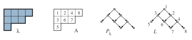
Figure 1.1: Young diagram $\lambda=(4,3,1)$, standard Young tableau $A\in\operatorname{{\rm SYT}}(\lambda)$, poset $P_{\lambda}$, and the corresponding linear extension $L\in\mathcal{L}(P_{\lambda})$.

We state our results, roughly, from less general to more general. Let  $\alpha=(\alpha_{1},\ldots,\alpha_{d})\in\mathbb{R}_{+}^{d}$, $\alpha_{1}\geq\ldots\geq\alpha_{d}\geq 0$, and  $|\alpha|=1$, where  $|\alpha|:=\alpha_{1}+\ldots+\alpha_{d}$. Such $\alpha$ are called Thoma sequences. Define a Thoma–Vershik–Kerov (TVK) $\alpha$-shape  $\lambda\simeq\alpha\hskip 0.85355ptn$, to be partition  $\lambda=(\lambda_{1},\ldots,\lambda_{d})$, with  $\lambda_{i}=\lfloor\alpha_{i}n\rfloor$, for all  $1\leq i\leq d$. Note that  $|\lambda|=n-O(1)$  in this case.

Theorem 1.2.

Fix $d\geq 2$. For every Thoma sequence  $\alpha\in\mathbb{R}^{d}_{>0}$, there is universal constant  $C_{\alpha}$, s.t.

$$\delta\bigl{(}P_{\lambda}\bigr{)}\hskip 1.70709pt\leq\hskip 1.70709pt\frac{C_{\alpha}}{\sqrt{n}}\,,$$

where  $\lambda\simeq\alpha\hskip 0.85355ptn$  is a TVK  $\alpha$-shape.

We say that a partition $\lambda\vdash n$ is  $\varepsilon$-thick, if the smallest part  $\lambda_{d}\geq\varepsilon\hskip 0.85355ptn$, where $d=\ell(\lambda)$.

Theorem 1.3.

Fix $d\geq 2$. For every $\varepsilon>0$, there is a universal constant $C_{d,\varepsilon}$, such that for every $\varepsilon$-thick partition $\lambda\vdash n$ with $\ell(\lambda)=d$ parts, we have:

$$\delta\bigl{(}P_{\lambda}\bigr{)}\hskip 1.70709pt\leq\hskip 1.70709pt\frac{C_{d,\varepsilon}}{\sqrt{n}}\,.$$

Clearly, every TVK $\alpha$-shape is $\varepsilon$-thick when   $0<\varepsilon<\alpha_{d}$, and $n$ is large enough. Thus, Theorem 1.3 can be viewed as an advanced generalization of Theorem 1.2.

Let  $\lambda=(\lambda_{1},\ldots,\lambda_{d})$,  $\mu=(\mu_{1},\ldots,\mu_{d})$  be two partitions with at most $d$ parts, and such that  $|\lambda/\mu|:=|\lambda|-|\mu|=n$. We write  $\mu\subset\lambda$, if $\mu_{i}\leq\lambda_{i}$ for all $1\leq i\leq d$, and refer to $\lambda/\mu$ as skew partition (see Figure 1.2). Since poset $P_{\mu}$ is a subposet of $P_{\lambda}$, poset  $P_{\lambda/\mu}$  is defined as their difference.

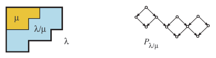
Figure 1.2: Skew Young diagram $\lambda/\mu$ and poset $P_{\lambda/\mu}$, where $\lambda=(5,5,4,2)$ and $\mu=(3,2,0,0)$.

Let  $\alpha=(\alpha_{1},\ldots,\alpha_{d})$, $\beta=(\beta_{1},\ldots,\beta_{d})\in\mathbb{R}_{+}^{d}$, $\alpha_{1}\geq\alpha_{2}\geq\ldots\geq\alpha_{d}$, $\beta_{1}\geq\ldots\geq\beta_{d}$, $\beta_{i}\leq\alpha_{i}$ for all $1\leq i\leq d$, and $|\alpha|-|\beta|=1$. Such $(\alpha,\beta)$ are called Thoma pairs. Define a TVK $(\alpha,\beta)$-shape to be the skew partition  $\lambda/\mu$, where  $\lambda\simeq\alpha\hskip 0.85355ptn$  and  $\mu\simeq\beta\hskip 0.85355ptn$. Note that  $|\lambda/\mu|=n+O(1)$  in this case.

Theorem 1.4.

Fix $d\geq 2$. For every Thoma pair  $(\alpha,\beta)$, with  $\alpha\in\mathbb{R}^{d}_{>0}$,  $\beta\in\mathbb{R}^{d}_{+}$, there is a universal constant $C_{\alpha,\beta}$, s.t.

$$\delta\bigl{(}P_{\lambda/\mu}\bigr{)}\hskip 1.70709pt\leq\hskip 1.70709pt\frac{C_{\alpha,\beta}}{\sqrt{n}}\,,$$

where  $\lambda/\mu$ is a TVK  $(\alpha,\beta)$-shape, i.e.  $\lambda\simeq\alpha\hskip 0.85355ptn$,  $\mu\simeq\beta\hskip 0.85355ptn$.

When  $\beta=(0,\ldots,0)$, we obtain Theorem 1.2 as a special case. We can now state our main result, the analogue of Theorem 1.3 for skew shapes.

We say that a partition $\lambda$ is  $\varepsilon$-smooth, if $\lambda$ is  $\varepsilon$-thick, and  $\lambda_{i}-\lambda_{i+1}\geq\varepsilon\hskip 0.85355ptn$, for all $1\leq i<d$. For brevity, we say that a skew partition $\lambda/\mu$ is $\varepsilon$-smooth if $\lambda$ is $\varepsilon$-smooth. Note that, despite the notation, this condition does not impose any restriction on $\mu$.

Theorem 1.5 (Main theorem).

Fix $d\geq 2$. For every $\varepsilon>0$, there is a universal constant $C_{d,\varepsilon}$, such that for every $\varepsilon$-smooth skew partition $\lambda/\mu\vdash n$, with $\ell(\lambda)=d$, we have:

$$\delta\bigl{(}P_{\lambda/\mu}\bigr{)}\hskip 1.70709pt\leq\hskip 1.70709pt\frac{C_{d,\varepsilon}}{\sqrt{n}}\,.$$

In the TVK case, when $\alpha_{1}>\ldots>\alpha_{d}>0$, we obtain Theorem 1.4. However, when the inequalities are non-strict, there is no such implication. Similarly, Theorem 1.5 generalizes Theorem 1.3 for $\mu=\varnothing$, and $\lambda$ is $\varepsilon$-smooth.

The results are proved by using random walks estimates and the technique Morales and the last two authors recently developed in a series of papers [MPP1]–[MPP4] on the Naruse hook-length formula (NHLF). Roughly, in order to estimate the sorting probabilities  $\delta\bigl{(}P_{\lambda}\hskip 0.85355pt;\hskip 1.70709ptx,\hskip 1.70709pty\bigr{)}$, we need very careful bounds on the number of standard Young tableaux  $f(\lambda/\nu):=|\operatorname{{\rm SYT}}(\lambda/\nu)|=e\bigl{(}P_{\lambda/\nu}\bigr{)}$ for the typical $\nu\subset\lambda$ obtained after removing $x$ and/or $y$ from $\lambda$. The NHLF gives a useful technical tool, which combined with various asymptotic estimates implies the result. We postpone further discussion of our results until after a brief literature review.

1.3 Prior work on sorting probability

The  $\frac{1}{3}$ – $\frac{2}{3}$  Conjecture 1.1 was proposed independently by Kislitsyn [Kis68] and Fredman [Fre75] in the context of sorting under partial information. The name is motivated by the following attractive equivalent formulation. In notation of (1.2), for every $P=(X,\prec)$ that is not a chain, there exist elements $x,y\in X$, such that

$$\frac{1}{3}\,\leq\,{\text{\bf P}}\bigl{[}L(x)<L(y)\bigr{]}\,\leq\,\frac{2}{3}\hskip 1.70709pt.$$ (1.3)

A major breakthrough was made by Kahn and Saks [KS84], who proved (1.3) with slightly weaker constants  $\frac{3}{11}-\frac{8}{11}$ . In our notation, they showed that  $\delta(P)\leq\frac{5}{11}\approx 0.4545$  for all finite $P$. A much simplified geometric proof (with a slightly weaker bound) was given later in [KL91]. By utilizing technical combinatorial tools, the Kahn–Saks bound was slightly improved in [BFT95] to  $\delta(P)\leq\frac{1}{\sqrt{5}}\approx 0.4472$, where it currently stands. For more on the history and various related results, we refer the reader to a dated but very useful survey [Bri99].

While the conjecture does not ask for an efficient algorithm for finding the desired elements $x,y\in X$, a nearly optimal sorting algorithm using  $O\bigl{(}\log e(P)\bigr{)}$  comparisons was found in [KK95]. See also [C+13] for a simpler version.

Note that the bound  $\delta(P)\leq\frac{1}{3}$  in the conjecture is tight for a 3-element poset that is a union of a $2$-chain and a single element. The effort to establish the conjecture and improve the constants remains very active. First, Linial [Lin84] proved that  $\delta(P)\leq\frac{1}{3}$  for posets of width $2$, where $\mathrm{width}(P)$ is the size of the maximal antichain in $P$. In this class, Aigner showed that the tight bound  $\delta(P)=\frac{1}{3}$  can come only from decomposable posets, and Sah [Sah21] recently improved the bound to a slightly lower bound  $\delta(P)<0.3225$ in the indecomposable case (see also [Chen18]).

Conjecture 1.1 was further established for several other classes of posets, including semiorders [Bri89], $N$-free posets [Zag12], height 2 posets [TGF92], and posets whose cover graph is a forest [Zag19]. For posets with a nontrivial automorphism the conjecture was proved by Pouzet, see [GHP87], and a stronger bound  $\delta(P)<1-\frac{2}{e}\approx 0.2642$  was shown by Saks [Saks85]. Closer to the subject of this paper, Olson and Sagan [OS18] recently applied Linial’s approach to establish Conjecture 1.1 for all Young diagrams and skew Young diagrams.

There are very few results proving that  $\delta(P_{n})\to 0$  as  $n\to\infty$  for a sequence  $\{P_{n}\}$  of posets on $n$ elements. Some of them are motivated by the following interesting conjecture of Kahn and Sacks [KS84].

Conjecture 1.6 (Kahn–Saks).

Let $\eta(d)$ denotes the supremum of $\delta(P)$ over all finite posets $P$ of width $d$. Then  $\eta(d)\to 0$  as  $d\to\infty$.

The most notable result in this direction is due to Komlós [Kom90], who proved it for height $2$ posets, as well as posets with  $n/f(n)$  minimal elements, for some undetermined, but possibly very slowly growing function  $f(n)=\omega(1)$. Similarly, Korshunov [Kor94] proved that Conjecture 1.6 holds for random posets, which are known to have height $3$ w.h.p. [KR75]. Note that these are the opposite extremes to our setting, as we consider posets $P_{\lambda/\mu}$ with width  $d=O(1)$  and height  $\Theta(n)$, see also $\S$13.1.

Before we conclude, let us note that for general posets, counting the number $e(P)$ of linear extensions, as well as computing the sorting probability $\delta(P)$, is #P-complete [BW91]. Thus, there is little hope of getting good asymptotic bounds on $\delta(P)$, except possibly for one of several notions of “random poset” [Bri93] and “large poset” [Jan11]. In fact, the same complexity results hold for counting linear extensions of general $2$-dimensional posets, as well as for posets of height $2$; both results are recently proved in [DP18]. This makes (skew) Young diagrams refreshingly accessible in comparison.

1.4 Prior work on asymptotics for standard Young tableaux

The combinatorics of standard Young tableaux is a classical subject, but until relatively recently, much of the work was on exact counting rather than on asymptotics and probabilistic aspects.

The hook-length formula (HLF) gives an explicit product formula for  $e(P_{\lambda})=|\operatorname{{\rm SYT}}(\lambda)|$, see e.g. [Sta99]. In the stable limit shape, the Young diagram $\lambda$ scaled by  $\frac{1}{\sqrt{n}}$  in both directions $\to\pi$, a curve of area 1. Then the HLF gives a tight asymptotic bound for  $e(P_{\lambda})$  via hook integral [VK81] (see also [MPP4]). Feit’s determinant formula is an exact formula for $f(\lambda/\mu)$, which can also be derived from the Jacobi–Trudi identity for skew shapes, see e.g. [Sta99]. Unfortunately, its determinantal nature makes finding exact asymptotics exceedingly difficult, see e.g. [BR10, MPP4].

For large skew shapes, Okounkov–Olshanski [OO98] and Stanley [Sta03] computed the asymptotics of $f(\lambda/\mu)$ for fixed $\mu$, as $|\lambda|\to\infty$. Both papers rely on the factorial Schur functions introduced by Macdonald in [Mac92, $\S$6]. The Naruse hook-length formula (NHLF) was introduced by Hiroshi Naruse in a talk in 2014, and given multiple proofs and generalizations in [MPP1, MPP2]. While the formula itself is algebro-geometric in nature, coming from the equivariant cohomology of the Grassmannian, some of the proofs are direct and combinatorial, using factorial Schur functions and explicit bijections [Kon, MPP1, MPP2] (see also [Pak21] for an overview).

In [MPP4], Morales–Pak–Panova used the NHLF and the hook integral approach to prove an exact asymptotic formula for $f(\lambda/\mu)$ when $\lambda/\mu$ have a TVK $(\alpha,\beta)$-shape. In [MPT18], based on a bijection with lozenge tilings given in [MPP3] and the variational principle in [CKP01], Morales–Pak–Tassy proved an asymptotic formula for $f(\lambda/\mu)$ when both $\lambda$ and $\mu$ have a stable limit shape. In a parallel investigation, Pittel–Romik [PR07] found limit curves for the shape of random Young tableaux of a rectangle. Most recently, Sun [Sun18] established existence of such limit curves for general skew stable limit shapes.

1.5 Some examples

The main difficulty in estimating the sorting probability is finding the “right” sorting elements $x,y\in X$, such that, even when suboptimal, still give a good bound for  $\delta(P;\hskip 0.85355ptx,y)$. To better understand this issue, let us illustrate the sorting probability in some simple examples.

First, take $\lambda=(n,1)$ and $\mu=(1)$. Then poset $P_{\lambda/\mu}$ consists of two chains, of length $1$ and $(n-1)$. There is an easy optimal pair of elements $x=(1,\lfloor\frac{n+1}{2}\rfloor)$ and $y=(2,1)$. Then  $\delta(P_{\lambda/\mu})=0$  for even $n$, and  $\delta(P_{\lambda/\mu})=\frac{1}{n}$  for odd $n$.  Similarly, let $\lambda=(n,2)$ and $\mu=(2)$. The poset $P_{\lambda/\mu}$ again consists of two chains, of length $2$ and $(n-2)$. In this case, the $x$ as above give suboptimal  $\delta(P_{\lambda/\mu};\hskip 1.70709ptx,y)\sim\frac{1}{2}$. Perhaps counterintuitively, the optimal sorting elements are  $y=(2,1)$  and  $x=(1,m)$, where  $m=n(1-\frac{1}{\sqrt{2}})+O(1)$. We have  $\delta(P_{\lambda/\mu};\hskip 1.70709ptx,y)=\Theta(\frac{1}{n})$  bound in this case. We generalize this example in $\S$3.2.

Now let $\lambda=(m,m)$, $\mu=\varnothing$, $n=2m$. We have $f(\lambda/\mu)=|\operatorname{{\rm SYT}}(m,m)|=\frac{1}{m+1}\binom{2m}{m}$, the Catalan number. One can check in this case that  $\delta(P_{\lambda/\mu};\hskip 1.70709ptx,y)=\Omega(1)$ for $y=(2,1)$ and every $x=(1,i)$. In fact, the bounds that work in this case are given by  $x=\bigl{(}1,\frac{m}{2}+k\bigr{)}$  and  $y=\bigl{(}2,\frac{m}{2}-k\bigr{)}$, for some  $k=\Theta(\sqrt{m})$. We prove in [CPP21] that  $\delta(P_{\lambda/\mu})=O\bigl{(}n^{-5/4}\bigr{)}$  by a direct asymptotic argument. A weaker  $O\bigl{(}\frac{1}{\sqrt{n}}\bigr{)}$  bound can be proved via standard bijection from standard Young tableaux $A\in\operatorname{{\rm SYT}}(m,m)$ and Dyck paths  $(0,0)\to(m,m)$, which in the limit  $m\to\infty$  converge to the Brownian excursion (see e.g. [Pit06]). This is the motivational example for this paper.

1.6 Our work in context

The differences between various approaches can now be explained in the way the authors look for the sorting elements. In [Lin84], Linial takes $P$ of width two, breaks it into two chains, takes $x$ to be the minimal element in one of them and looks for $y$ in another chain. As the previous examples show, this approach can never give  $\delta(P)=o(1)$  for general Young tableaux even with two rows. This approach has been influential, and was later refined and applied in a more general settings, see e.g. [Bri89, Zag12].

In [KS84] and followup papers [BFT95, KL91, Kom90, Zag12], a more complicated pigeonhole principle is used, at the end of which there is no clear picture of what sorting elements are chosen. In fact, the geometric approach in [KS84, KL91] can never give  $\delta(P)=o(1)$, as they also point out, cf. [Saks85]. The paper most relevant to our paper is [OS18], where the authors look for elements $x,y$ on the boundary  $\partial\lambda$, and apply the pigeonhole principle, Linial-style. Already in the Catalan example this approach cannot be used to prove that  $\delta(P;\hskip 0.85355ptx,y)=o(1)$.

Now, following [PR07, Sun18], let  $\lambda\vdash n$  be the stable limit shape. It is natural to take $x$ and $y$ from the same limit curve  $C_{\lambda}(\alpha):=\partial\{(i,j)\in\lambda,\hskip 1.70709ptA(i,j)\leq\alpha\hskip 0.85355ptn\}$, where  $0<\alpha<1$, and  $A\in\operatorname{{\rm SYT}}(\lambda)$  is a uniform standard Young tableau of shape $\lambda$. An example of these limit curves is given in Figure 1.3. Since the curves $C_{\lambda}(\alpha)$ have  $\Theta(\sqrt{n})$  elements, and all $(i,j)\in C_{\lambda}(\alpha)$ can be permuted nearly independently, this could in principle give a small sorting probability. Making this precise would be both interesting and challenging, but this approach fails in our case, since we have  $d=O(1)$  rows. It does have a few heuristic implications.

Figure 1.3: The limit curves in a $d\times 2d$ rectangle (created by Dan Romik, April 2020).

On the one hand, there are likely to be many good sorting pairs of elements $x=(i,j)$, $y=(i^{\prime},j^{\prime})$, for all $i<j$. On the other hand, in general, the limit curves do not have a closed-form formula of any kind, and arise as the solution of a variational problem [Sun18]. The same holds for the asymptotics of  $f(\lambda/\mu)$ [MPT18]. As a consequence, we are essentially forced to make an indirect argument, which proves the result without explicitly specifying the exact location of $x,y$ in $\lambda$.

Our approach is based on a combination of tools and ideas from algebraic combinatorics and discrete probability. The general philosophy is somewhat similar to the pigeonhole principle of Linial [Lin84], in the sense that we find a sorting pair  $x=(1,a)$  and  $y=(2,b)$  by searching over suitable choices of $a,b$. As in the Catalan case, we start with extreme cases $a=\lambda_{1}$, $b=\mu_{2}+1$, and decrease $(a-b)$ until the sorting probabilities of $x$ and $y$ becomes small. The main difficulty, of course, is estimating these sorting probabilities.

In fact, by analogy with the Catalan example, one can interpret random standard Young tableaux as random walks from  $(0,\ldots,0)$  to  $(\lambda_{1},\ldots,\lambda_{d})$, which are confined to a certain simplex region in $\mathbb{N}^{d}$ defined by combinatorial constraints. The sorting probability  $\delta(P_{\lambda/\mu};\hskip 1.70709ptx,y)$  can then be interpreted as the probability the walk passes below versus above of certain codimension-2 subspace. These probabilities are then bounded by comparing the simplex-confined lattice walk with the usual (unconstrained) lattice walk. This comparison is based on delicate estimates which largely rely on the Schur functions technology combined with the NHLF. This technical part occupies much of the paper.

1.7 Structure of the paper

We begin by reviewing standard definitions and notation in Section 2, where we also include a number of basic results in Algebraic Combinatorics and Discrete Probability. In the Warmup Section 3 we prove the  $\frac{1}{3}$ – $\frac{2}{3}$  Conjecture 1.1 for all Young diagrams. This is a known result, but the proof we give is new and the tools are a precursor of the proof of the Main Theorem 1.5. We also show how these tools easily give an upper bound on the sorting probability $\delta(P_{\lambda})$, for $n-\lambda_{1}=o(n)$, where  $n=|\lambda|$. In fact, this short section has both the style and the flavor of the rest of the paper, cf. $\S$4.8.

In Section 4, we give key new definitions which allow us to state the Main Lemma 4.3, and two bounds Lemmas 4.4 and 4.5 on the number  $f(\lambda/\mu)$  of standard Young tableaux of shape $\lambda/\mu$. The proofs of these lemmas occupy much of the paper. The technical outline of these proofs is the given in $\S$4.7, so below we only give the structure of the paper in the broadest terms.

First, in Sections 5–7, we develop the technology of lattice path probabilities and their estimates, which culminates with the proof of Main Lemma 4.3 in Section 7. Then, in Section 8, we develop the technology of Young tableaux estimates, which allows us to prove Theorem 1.3 in Section 9. We then prove Lemma 4.4 and Main Theorem 1.5 in Section 10. Finally, Lemma 4.5 and Theorem 1.4 are proved in Section 11.

We conclude with Section 12, where we state several conjectures and open problems motivated by our results. We present final remarks in Section 13.

2 Definitions, notation and background results

2.1 Standard conventions

We fix the number of rows  $d\geq 2$  throughout the paper. We consider only posets $P=(X,\prec)$ corresponding to partitions $\lambda\vdash n$, or skew partitions  $\lambda/\mu\vdash n$. Unless stated otherwise, we have  $|X|=n$.

We use  $[n]=\{1,\ldots,n\}$,  $\mathbb{N}=\{0,1,2,\ldots\}$,  $\mathbb{Z}_{+}=\{1,2,\ldots\}$,  $\mathbb{R}_{+}=\{x\geq 0\}$, and  $\mathbb{R}_{>0}=\{x>0\}$. We denote by  $\mathbb{P}_{d}\subset\mathbb{N}^{d}$  the set of partitions  $(\lambda_{1},\ldots,\lambda_{d})$, where  $\lambda_{1}\geq\ldots\geq\lambda_{d}\geq 0$, and  $\lambda_{i}\in\mathbb{N}$. We write  $(a_{1},\ldots,a_{d})\trianglerighteq(b_{1},\ldots,b_{d})$, when  $a_{1}\geq b_{1}$,  $a_{1}+a_{2}\geq b_{1}+b_{2}$,  … , and  $a_{1}+\ldots+a_{d}=b_{1}+\ldots+b_{d}$.

2.2 Standard Young tableaux

We adopt standard notation in the area. See e.g. [Mac95, Sag01, Sta99] for these results and further references.

Let  $\lambda=(\lambda_{1},\ldots,\lambda_{d})\vdash n$,  $\lambda_{1}\geq\ldots\geq\lambda_{d}\geq 0$, be an integer partition of $n$. Here  $n=|\lambda|:=\lambda_{1}+\ldots+\lambda_{d}$  denotes the size of $\lambda$, and $\ell(\lambda)\leq d$ is the number of parts of $\lambda$. We use $\lambda^{\prime}$ to denote a conjugate partition whose parts are the column lengths of the diagram $\lambda$.

A skew partition $\lambda/\mu$ is a pair of partitions $\lambda=(\lambda_{1},\ldots,\lambda_{d})$, $\mu=(\mu_{1},\ldots,\mu_{d})$, such that $\mu_{i}\leq\lambda_{i}$. In the vector notation above, $\lambda,\mu\in\mathbb{P}_{d}$, and $\lambda-\mu\in\mathbb{N}^{d}$. The empty partition is $\mu=(0,\ldots,0)$, which we also denote $\varnothing$, e.g. $\lambda/\varnothing=\lambda$. The size $|\lambda/\mu|:=|\lambda|-|\mu|$; we write $\lambda/\mu\vdash n$ for $|\lambda/\mu|=n$.

A Young diagram (shape), which we also denote by $\lambda$, is a set of squares $(i,j)\in\mathbb{N}^{2}$, such that  $1\leq i\leq d$, and  $1\leq j\leq\lambda_{i}$. Similarly, a skew Young diagram, which we also denote by $\lambda/\mu$, is a set of squares $(i,j)\in\mathbb{N}^{2}$, such that  $1\leq i\leq d$  and  $\mu_{i}<j\leq\lambda_{i}$. It can in principle have empty rows or be disconnected, although such cases are less interesting. We adopt the English notation, where $i$ increases downwards, and $j$ from left to right, as in Figure 1.1.

A standard Young tableau of shape $\lambda/\mu$ is a bijection  $A:\lambda/\mu\to[n]$, which increases in rows and columns, see Figure 1.1. We use $\operatorname{{\rm SYT}}(\lambda)$ to denote the set of standard Young tableaux of shape $\lambda/\mu$. As in the introduction, we use $P_{\lambda/\mu}=(\lambda/\mu,\prec)$ to denote the poset on the set of squares of $\lambda/\mu$, with the partial order defined by  $(i,j)\preccurlyeq(i^{\prime},j^{\prime})$  if and only if  $i\leq i^{\prime}$ and $j\leq j^{\prime}$. This is a standard definition of a $2$-dimensional poset associated with a set of points in the plane, see e.g. [Tro95].

Recall that the linear extensions $\mathcal{L}(P_{\lambda/\mu})$ are in natural bijection with the set  $\operatorname{{\rm SYT}}(\lambda)$  of standard Young tableaux. Whenever clear, we will use the latter from this point on. Denote by $\operatorname{{\text{\bf P}}_{\lambda/\mu}}$ the uniform probability measure on $\operatorname{{\rm SYT}}(\lambda/\mu)$. To simplify and unify the notation, from now on we use

$$f(\lambda/\mu)\,:=\,\bigl{|}\operatorname{{\rm SYT}}(\lambda/\mu)\bigr{|}\hskip 1.70709pt=\hskip 1.70709pte\bigl{(}P_{\lambda/\mu}\bigr{)}\hskip 1.70709pt=\hskip 1.70709pt\bigl{|}\mathcal{L}\bigl{(}P_{\lambda/\mu}\bigr{)}\bigr{|}.$$

For straight shapes $\lambda\vdash n$, we have the Frobenius formula:

$$f(\lambda)\,=\,\frac{n!}{\lambda_{1}!\hskip 1.70709pt\cdots\hskip 0.85355pt\lambda_{d}!}\hskip 1.70709pt\prod_{1\leqslant i<j\leqslant d}\frac{\lambda_{i}-\lambda_{j}+j-i}{\lambda_{i}+j-i}\,,$$ (2.1)

see e.g. [FRT54] (cf. [Mac92, Ex. 1.1] and [Sta99, Lemma 7.21.1]).

2.3 Schur polynomials

A semistandard Young tableau of shape $\lambda$ is an map  $A:\lambda\to\mathbb{Z}_{+}$, such that $A$ is weakly increasing in rows and strictly increasing in columns. We write $\operatorname{SSYT}(\lambda,d)$ for the set of such tableaux with all entries $\leq d$. The Schur polynomial is a symmetric polynomial defined as

$$s_{\mu}(x_{1},\ldots,x_{d})\,:=\,\det\bigl{(}x_{j}^{m_{i}}\bigr{)}_{i,j=1}^{d}\,\prod_{1\leq i<j\leq d}(x_{i}-x_{j})^{-1}\hskip 1.70709pt,$$ (2.2)

where  $m_{i}=m_{i}(\mu):=\mu_{i}+d-i$. We call  $(m_{1},\ldots,m_{d})=\mu+(d-1,\ldots,1,0)$  the shifted partition $\mu$.

The combinatorics of Schur functions is given by

$$s_{\lambda}(x_{1},\ldots,x_{d})\,:=\,\sum_{A\in\operatorname{SSYT}(\lambda,d)}\,\prod_{(i,j)\in\lambda}\hskip 1.70709ptx_{A(i,j)}\,=\,\sum_{A\in\operatorname{SSYT}(\lambda,d)}\,\prod_{i=1}^{d}\hskip 1.70709pt(x_{i})^{t_{i}(A)}\hskip 0.85355pt,$$ (2.3)

where

$$t_{i}(A)\,:=\,\bigl{|}\bigl{\{}(j,k)\in\lambda/\mu\,\mid\,A(j,k)=i\bigr{\}}\bigr{|}\hskip 1.70709pt,\qquad 1\leq i\leq d\hskip 0.85355pt.$$ (2.4)

The product formula below is classical and follows from (2.2) and (2.3):

$$s_{\mu}(1,\ldots,1)\,=\,\bigl{|}\operatorname{SSYT}(\lambda,d)\bigr{|}\,=\,\prod_{1\leqslant i<j\leqslant d}\frac{m_{i}-m_{j}}{j-i}\hskip 1.70709pt.$$ (2.5)

2.4 Hook-length formulas

The hook-length of square  $(i,j)\in\lambda$  is defined as

$$h_{\lambda}(i,j)\hskip 1.70709pt:=\hskip 1.70709pt\lambda_{i}-j+\lambda_{j}^{\prime}-i+1\hskip 0.85355pt.$$ (2.6)

The hook-length formula (HLF) [FRT54] (see also [Sag01, Sta99]), is a product formula for the number of standard Young tableaux of straight shape:

$$f(\lambda)\,=\,n!\hskip 1.70709pt\prod_{(i,j)\in\lambda}\hskip 1.70709pt\frac{1}{h_{\lambda}(i,j)}\hskip 1.70709pt.$$ (2.7)

For skew Young diagrams, the number $f(\lambda/\mu)$ can be determined by the Naruse hook-length formula (NHLF), see [MPP1, MPP2]. Let $D\subset\lambda$ be a subset of squares with the same number of squares in each diagonal as $\mu$. A subset $D$ is called an excited diagram if and only if the relation $\preccurlyeq$ on squares of $\mu$ holds for the corresponding squares in $D$. Denote by  $\operatorname{\mathrm{ED}}(\lambda/\mu)$  the set excited diagram of shape $\lambda/\mu$. As shown in [MPP1], all $D\in\operatorname{\mathrm{ED}}(\lambda/\mu)$ can be obtained from $\mu$ by a sequence of excited moves: $(i,j)\to(i+1,j+1)$, for some $(i,j)\in D$, s.t. $(i+1,j),\hskip 0.85355pt(i,j+1)\notin D$.

Theorem 2.1 (NHLF [MPP1]).

For all  $\lambda/\mu\vdash n$, we have:

$$f(\lambda/\mu)\,=\,\,n!\hskip 1.70709pt\sum_{D\in\hskip 0.85355pt\operatorname{\mathrm{ED}}(\lambda/\mu)}\prod_{(i,j)\in\lambda\smallsetminus D}\hskip 1.70709pt\frac{1}{h_{\lambda}(i,j)}\hskip 1.70709pt.$$ (2.8)

When $\mu=\varnothing$, we obtain the HLF (2.7). The next result is a consequence of the NHLF. Define

$$F(\lambda/\mu)\,:=\,n!\hskip 1.70709pt\prod_{(i,j)\in\lambda/\mu}\hskip 1.70709pt\frac{1}{h_{\lambda}(i,j)}\,.$$ (2.9)

Theorem 2.2 ([MPP4, Thm 3.3]).

Let $\lambda/\mu\vdash n$, $\ell(\lambda)\leq d$. Then

$$F(\lambda/\mu)\,\leq\,f(\lambda/\mu)\,\leq\,\bigl{|}\operatorname{\mathrm{ED}}(\lambda/\mu)\bigr{|}\hskip 0.85355pt\cdot\hskip 0.85355ptF(\lambda/\mu)\hskip 0.85355pt.$$

In an effort to quantify excited diagrams, we follow an equivalent definition given in [MPP1, $\S$3.3]. A flagged tableau of shape $\lambda/\mu$ is a tableaux  $T\in\operatorname{SSYT}(\mu)$, such that

$$j\hskip 0.85355pt+\hskip 0.85355ptT(i,j)\hskip 0.85355pt-\hskip 0.85355pti\hskip 1.70709pt\leq\hskip 1.70709pt\lambda_{T(i,j)}\,,\quad\text{for all}\ \hskip 1.70709pt(i,j)\in\mu\hskip 0.85355pt.$$ (2.10)

The corresponding excited diagram is obtained by moving $(i,j)$ for  $T(i,j)-i$  steps down the southeast diagonal. The above inequality is a constraint that  $D\subset\lambda$. We denote by  $\operatorname{\mathrm{FT}}(\lambda/\mu)$  the set of flagged tableaux of shape $\lambda/\mu$, so  $|\operatorname{\mathrm{FT}}(\lambda/\mu)|=|\operatorname{\mathrm{ED}}(\lambda/\mu)|$.

Theorem 2.3 (Flagged NHLF [MPP1]).

For all  $\lambda/\mu\vdash n$, we have:

$$f(\lambda/\mu)\,=\,\,n!\hskip 1.70709pt\Biggl{[}\prod_{(i,j)\in\lambda}\hskip 1.70709pt\frac{1}{h_{\lambda}(i,j)}\Biggr{]}\hskip 1.70709pt\sum_{T\in\operatorname{\mathrm{FT}}(\lambda/\mu)}\ \prod_{(i,j)\in\mu}h_{\lambda}\bigl{(}T(i,j),j+T(i,j)-i\bigr{)}.$$ (2.11)

2.5 Bounds on binomial coefficients

Recall an effective version of the Stirling formula:

$$\sqrt{2\pi}\hskip 1.70709ptn^{n+\frac{1}{2}}\hskip 0.85355pte^{-n}\hskip 1.70709pt\leq\hskip 1.70709ptn!\hskip 1.70709pt\leq\hskip 1.70709ptn^{n+\frac{1}{2}}\hskip 0.85355pte^{1-n}\hskip 0.85355pt.$$ (2.12)

This implies the following standard result:

Proposition 2.4.

Let $a,b$ be integers such that $a>b>0$. Then

$$\frac{\sqrt{2\pi}}{e^{2}}\hskip 1.70709pt\sqrt{\frac{a}{b(a-b)}}\hskip 1.70709pt\exp\bigl{(}a\hskip 0.85355ptH(b/a)\bigr{)}\,\leq\,\binom{a}{b}\,\leq\,\frac{e}{2\pi}\hskip 1.70709pt\sqrt{\frac{a}{b(a-b)}}\hskip 1.70709pt\exp\bigl{(}a\hskip 0.85355ptH(b/a)\bigr{)}\hskip 0.85355pt,$$

where  $H(r)\hskip 0.85355pt:=\hskip 0.85355pt-r\hskip 0.85355pt\log r\hskip 0.85355pt-\hskip 0.85355pt(1-r)\hskip 0.85355pt\log(1-r)$  is the  binary entropy function.

2.6 Concentration inequalities

Consider a simple random walk  $\textbf{{X}}=\bigl{(}X_{t}\bigr{)}_{t\geq 0}$  on  $\mathbb{R}^{d}$, with steps $V=\{v_{1},\ldots,v_{k}\}\subset\mathbb{R}^{d}$ and probability distribution $Q$ on $[k]$:

$$X_{0}\hskip 1.70709pt=\hskip 1.70709ptO,\ \ X_{t+1}\hskip 1.70709pt=\hskip 1.70709ptX_{t}\hskip 1.70709pt+\hskip 1.70709ptv_{i}\hskip 1.70709pt,\quad\text{where \, $1\leq i\leq k$ \, \hskip 1.70709ptis chosen with probability \hskip 1.70709pt$q_{i}:=Q(i)$.}$$ (2.13)

We will use the following concentration inequality that applies in much more general situation.

Theorem 2.5 (Hoeffding’s inequality [Hoe63]).

Let $\textbf{{X}}=(X_{t})_{t\geq 0}$ be a random walk on $\operatorname{\mathbb{R}}^{d}$ with steps $V$ such that $\|v_{i}\|\leq 1$. Then, for every $t\geq 1$ and $c>0$ ,

$${\text{\bf P}}\bigl{[}\hskip 0.85355pt\|X_{t}-\operatorname{\mathbb{E}}[X_{t}]\hskip 0.85355pt\|\hskip 1.70709pt\geq\hskip 1.70709ptc\bigr{]}\ \leq\ 2\exp\left(-2c^{2}/t\right).$$

In $\S$5.5, we will use Hoeffding’s inequality for the set of steps  $E=\{e_{1},\ldots,e_{d}\}$  which forms the standard basis in $\mathbb{R}^{d}$, and a certain non-uniform distribution $Q$ on $[d]$.

3 Warmup

In this short section we give a new proof and an extension of the  $\frac{1}{3}$–$\frac{2}{3}$  Conjecture 1.1 for Young diagrams. We apply these to give an upper bound for the sorting probability for general Young diagrams.

3.1 General Young diagrams

The first part of the following theorem is the result by Olson and Sagan [OS18]. Below, we present a completely different proof of the result. In fact, our sorting pairs of elements are in a different location when compared to [OS18].

Theorem 3.1.

For every $\lambda\vdash n$, we have  $\delta(P_{\lambda})\leq\frac{1}{3}$. Moreover, $\delta(P_{\lambda};\hskip 0.85355ptx,y)\hskip 0.85355pt\leq\hskip 0.85355pt\frac{1}{3}$  for some  $x=(1,k)\in\lambda$  and  $y=(\ell,1)\in\lambda$.

As suggested by the second part of the Theorem, we need to estimate sorting probabilities for pairs of elements in the first row and the first column.

Lemma 3.2.

Let  $\lambda\vdash n$, and  $\operatorname{{\text{\bf P}}_{\lambda}}$  denote the probability over uniform standard Young tableaux  $A\in\operatorname{{\rm SYT}}(\lambda)$. Denote

$$q_{i} :=\,\operatorname{{\text{\bf P}}_{\lambda}}\bigl{[}\hskip 0.85355ptA(i,1)\hskip 1.70709pt<\hskip 1.70709ptA(1,2)\hskip 1.70709pt<\hskip 1.70709ptA(i+1,1)\hskip 0.85355pt\bigr{]}\hskip 0.85355pt,\quad 1\leq i\leq\ell-1\hskip 1.70709pt,\quad\text{and}$$

$$q_{\ell} :=\,\operatorname{{\text{\bf P}}_{\lambda}}\bigl{[}\hskip 0.85355ptA(\ell,1)\hskip 1.70709pt<\hskip 1.70709ptA(1,2)\hskip 0.85355pt\bigr{]}\hskip 0.85355pt,$$

where  $\ell=\ell(\lambda)$  is the length of the first column. Then  $q_{1}\geq\ldots\geq q_{\ell}$, and  $q_{1}+\ldots+q_{\ell}=1$.

We present two proofs of the lemma: the traditional Young tableaux proof and the proof via the Naruse hook-length formula (Theorem 2.3). The former proof is simpler while the latter is amenable for generalizations and asymptotic analysis. We recommend the reader study both proofs.

First proof of Lemma 3.2.

Since  $A(1,1)=1<A(1,2)$, the number  $A(1,2)$  must fall in exactly one of the intervals in the lemma. Thus, we have  $q_{1}+\ldots+q_{\ell}=1$.

Let  $A\in\operatorname{{\rm SYT}}(\lambda)$  be a standard Young tableau, such that  $A(k,1)<A(1,2)<A(k+1,1)$, for some  $1\leq k<\ell$. Then  $A(1,1)=1$, …, $A(k,1)=k$, and $A(1,2)=k+1$. The number of such tableaux $A$ is then equal to $f(\lambda/\mu^{k})$, where  $\mu^{k}=(2,1^{k-1})\vdash k+1$. In the notation of the lemma, we have:

$$q_{k}\,=\,\frac{f(\lambda/\mu^{k})}{f(\lambda)}\hskip 1.70709pt.$$ (3.1)

Clearly  $\mu^{k}\subset\mu^{k+1}$, and so  $\lambda/\mu^{k+1}\subset\lambda/\mu^{k}$. Then $f(\lambda/\mu^{k+1})$ is equal to the number of tableaux $A\in\operatorname{{\rm SYT}}\bigl{(}\lambda/\mu^{k}\bigr{)}$  with  $A(k,1)=1$. Therefore,  $f(\lambda/\mu^{k+1})\leq f(\lambda/\mu^{k})$  and  $q_{k+1}\leq q_{k}$. ∎

Second proof of Lemma 3.2.

We follow the first proof until (3.1). At this point, recall the Naruse hook-length formula (2.8):

$$f(\lambda/\mu)\,=\,(n-|\mu|)!\,\prod_{(i,j)\in\lambda}\hskip 1.70709pt\frac{1}{h_{\lambda}(i,j)}\,\sum_{D\in\operatorname{\mathrm{ED}}(\lambda/\mu)}\hskip 1.70709pt\prod_{(i,j)\in D}\hskip 1.70709pth_{\lambda}(i,j)\hskip 0.85355pt.$$

Combined with the hook-length formula (2.7), we have:

$$q_{k}\,=\,\frac{f(\lambda/\mu)}{f(\lambda)}\,=\,\frac{(n-k-1)!}{n!}\,\sum_{D\in\operatorname{\mathrm{ED}}(\lambda/\mu)}\hskip 1.70709pt\prod_{(i,j)\in D}\hskip 1.70709pth_{\lambda}(i,j)\hskip 0.85355pt.$$ (3.2)

Now, let  $\nu:=(2,1^{k})\vdash k+2$. We similarly have:

$$q_{k+1}\,=\,\frac{f(\lambda/\nu)}{f(\lambda)}\,=\,\frac{(n-k-2)!}{n!}\,\sum_{D^{\prime}\in\operatorname{\mathrm{ED}}(\lambda/\nu)}\hskip 1.70709pt\prod_{(i,j)\in D^{\prime}}\hskip 1.70709pth_{\lambda}(i,j)\hskip 0.85355pt.$$ (3.3)

Observe that excited diagrams $D^{\prime}\in\operatorname{\mathrm{ED}}(\lambda/\nu)$  are characterized by the locations of the squares  $x_{c}\in D^{\prime}$  in the diagonal  $\{i-j=c\}$, where  $-1\leq c\leq k$ (see Figure 3.1).

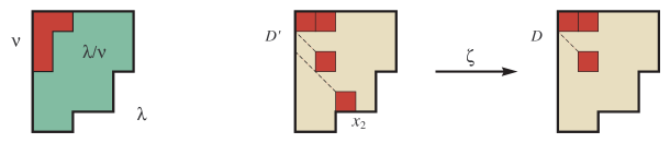
Figure 3.1: Skew Young diagram $\lambda/\nu$, where  $\lambda=(5,5,5,4,4,2)$  and  $\nu=(2,1,1)$.  Map ${\zeta}:D^{\prime}\to D$, where  $D^{\prime}\in\operatorname{\mathrm{ED}}(\lambda/\nu)$,  $D\in\operatorname{\mathrm{ED}}(\lambda/\mu)$, and  $D^{\prime}\smallsetminus D=x_{2}=(5,3)$.

Consider a map  ${\zeta}:\operatorname{\mathrm{ED}}(\lambda/\nu)\to\operatorname{\mathrm{ED}}(\lambda/\mu)$,  ${\zeta}(D^{\prime})=D$, where $D$ is obtained from $D^{\prime}$ by removing the square $x_{k}$. From above and by definition of excited diagrams, map ${\zeta}$ is well defined. This gives:

$$\sum_{D^{\prime}\in\operatorname{\mathrm{ED}}(\lambda/\nu)}\hskip 1.70709pt\prod_{(i,j)\in D^{\prime}}\hskip 1.70709pth_{\lambda}(i,j)\,=\,\sum_{D\in\operatorname{\mathrm{ED}}(\lambda/\mu)}\prod_{(i,j)\in D}\hskip 1.70709pth_{\lambda}(i,j)\,\sum_{\begin{subarray}{c}(i,j)\in\lambda,\,i-j=k\\ D\cup(i,j)\hskip 1.70709pt\in\hskip 1.70709pt\operatorname{\mathrm{ED}}(\lambda/\nu)\end{subarray}}\,h_{\lambda}(i,j)$$ (3.4)

The sum on the right is at most

$$h_{\lambda}(k+1,1)\hskip 1.70709pt+\hskip 1.70709pth_{\lambda}(k+2,2)\hskip 1.70709pt+\hskip 1.70709pt\ldots\,=\,\lambda_{k+1}\hskip 1.70709pt+\hskip 1.70709pt\ldots\hskip 1.70709pt+\hskip 1.70709pt\lambda_{\ell}\,\leq\,n\hskip 1.70709pt-\hskip 1.70709pt|\mu|\,=\,n-k-1\hskip 0.85355pt.$$ (3.5)

Combining these equations together, we obtain:

$$q_{k+1} =_{\eqref{eq:qk-formula}}\qquad\frac{(n-k-2)!}{n!}\,\sum_{D^{\prime}\in\operatorname{\mathrm{ED}}(\lambda/\nu)}\hskip 1.70709pt\prod_{(i,j)\in D^{\prime}}\hskip 1.70709pth_{\lambda}(i,j)$$

$$\leq_{\eqref{eq:ED-sum-formula}\,\eqref{eq:hook-sum-formula}}\ \frac{(n-k-2)!}{n!}\,\sum_{D\in\operatorname{\mathrm{ED}}(\lambda/\mu)}\,\hskip 1.70709pt\hskip 0.85355pt\prod_{(i,j)\in D}\hskip 1.70709pth_{\lambda}(i,j)\hskip 1.70709pt(n-k-1)\ =_{\eqref{eq:qk+1-formula}}\ q_{k}\,,$$

as desired. ∎

Proof of Theorem 3.1.

Without loss of generality, we can assume that

$$p_{1}\,:=\,\operatorname{{\text{\bf P}}_{\lambda}}\bigl{[}A(1,2)\hskip 1.70709pt<\hskip 1.70709ptA(2,1)\bigr{]}\,\leq\,\frac{1}{2}\hskip 1.70709pt,$$

since we can conjugate diagram $\lambda$, otherwise. If  $p_{1}\geq\frac{1}{3}$, this implies  $\delta(P_{\lambda};\hskip 0.85355ptx,y)\leq\frac{1}{3}$  for  $x=(1,2)$ and $y=(2,1)$, and proves the theorem.

Suppose now that  $p\leq\frac{1}{3}$. By the lemma, we have:

$$\frac{1}{3}\hskip 1.70709pt\geq\hskip 1.70709ptp_{1}\hskip 1.70709pt=\hskip 1.70709ptq_{1}\hskip 1.70709pt\geq\hskip 1.70709ptq_{2}\hskip 1.70709pt\geq\hskip 1.70709pt\ldots\hskip 1.70709pt\geq\hskip 1.70709ptq_{\ell}\hskip 0.85355pt.$$

Observe that

$$p_{k}\,:=\,\operatorname{{\text{\bf P}}_{\lambda}}\bigl{[}A(1,2)\hskip 1.70709pt<\hskip 1.70709ptA(k+1,1)\bigr{]}\,=\,q_{1}\hskip 1.70709pt+\hskip 1.70709pt\ldots\hskip 1.70709pt+\hskip 1.70709ptq_{k}\hskip 1.70709pt.$$

Since  $q_{k}\leq\frac{1}{3}$  and  $q_{1}+\ldots+q_{\ell}=1$  by the lemma, this implies that at least one of these probabilities  $p_{k}\in\bigl{[}\frac{1}{3},\frac{2}{3}\bigr{]}$. Therefore, the sorting probability  $\delta(P_{\lambda};\hskip 0.85355ptx,y)\leq\frac{1}{3}$  for  $x=(1,2)$  and  $y=(k+1,1)$, as desired. ∎

3.2 General upper bounds

For a partition  $\lambda\vdash n$  define the imbalance  $\textrm{q}(\lambda)$  as follows:

$$\textrm{q}(\lambda)\hskip 1.70709pt:=\hskip 1.70709pt\frac{1}{n(n-1)}\hskip 1.70709pt\sum_{i\leq j}\hskip 1.70709pth_{\lambda}(i,i)\hskip 0.85355pth_{\lambda}(j,j+1)\hskip 0.85355pt.$$ (3.6)

Note that

$$\sum_{i\leq j}\hskip 1.70709pth_{\lambda}(i,i)\hskip 0.85355pth_{\lambda}(j,j+1)\,\leq\,\sum_{i}\hskip 1.70709pth_{\lambda}(i,i)\,\sum_{j}h_{\lambda}(j,j+1)\,\leq\,n\hskip 0.85355pt(n-1)\hskip 0.85355pt,$$ (3.7)

so  $0\leq\textrm{q}(\lambda)\leq 1$.  The following result is a generalization of Theorem 3.1.

Theorem 3.3.

For every $\lambda\vdash n$, we have:

$$\delta(P_{\lambda})\,\leq\,\min\big{\{}\hskip 1.70709pt\textrm{q}(\lambda),\hskip 1.70709pt1-\textrm{q}(\lambda),\hskip 1.70709pt|1-2\hskip 0.85355pt\hskip 0.85355pt\textrm{q}(\lambda)|\hskip 1.70709pt\big{\}}.$$

Proof.

In the notation of the proof above, let  $k=1$,  $\mu=(2)$, and observe that excited diagrams  $D\in\operatorname{\mathrm{ED}}(\lambda/\mu)$  consist of two squares: $(i,i)$ and $(j,j+1)\in\lambda$, s.t. $1\leq i\leq j$. Therefore,

$$p_{1}\hskip 1.70709pt=\hskip 1.70709ptq_{1}\hskip 1.70709pt=\hskip 1.70709pt\frac{f(\lambda/\mu)}{f(\lambda)}\hskip 1.70709pt=\hskip 1.70709pt\frac{1}{n(n-1)}\hskip 1.70709pt\sum_{D\in\operatorname{\mathrm{ED}}(\lambda/\mu)}\hskip 1.70709pt\prod_{(i,j)\in D}\hskip 1.70709pth_{\lambda}(i,j)\,=_{\eqref{eq:imbalance}}\,\textrm{q}(\lambda)\hskip 0.85355pt.$$

There are three possibilities. First, if  $q_{1}\leq\frac{1}{3}$, then the sorting probability  $\delta(P_{\lambda})\leq q_{k}\leq q_{1}$. Similarly, if  $q_{1}\geq\frac{2}{3}$, by using  $\textrm{q}(\lambda^{\prime})=1-q_{1}$, we have  $\delta(P_{\lambda})\leq 1-\textrm{q}(\lambda)$. Finally, if  $\frac{1}{3}\leq q_{1}\leq\frac{2}{3}$, we have  $\delta(P_{\lambda})\leq|1-2\hskip 0.85355ptq_{1}|$  by definition of $p_{1}=q_{1}$. This implies the result. ∎

Lemma 3.4.

Let  $\lambda\vdash n$, and $m=n-\lambda_{1}$. Then:

$$\delta(P_{\lambda})\,\leq\,\frac{m\hskip 0.85355ptn\hskip 1.70709pt+\hskip 1.70709pt(m-1)(m-2)}{n(n-1)}\hskip 1.70709pt.$$

Proof.

We apply Theorem 3.3 to the conjugate partition $\lambda^{\prime}$. We have  $h_{\lambda^{\prime}}(1,1)\leq n$, and

$$\sum_{j\geq 1}\hskip 0.85355pth_{\lambda^{\prime}}(j,j+1)\,=\,\sum_{j\geq 1}\hskip 0.85355pth_{\lambda}(j+1,j)\,=\,m.$$

Thus, the first term $i=1$ of the summation (3.6) for the imbalance $\textrm{q}(\lambda^{\prime})$, is at most  $m\hskip 0.85355ptn$. The remaining terms with  $i\geq 2$  are equal to  $\textrm{q}(\tau^{\prime})$, where  $\tau=(\lambda_{2}-1,\lambda_{3}-1,\ldots)$  of size $\leq m-1$. We conclude:

$$\textrm{q}(\lambda^{\prime})\,\leq\,\frac{1}{n(n-1)}\hskip 1.70709pt\bigl{(}m\hskip 0.85355ptn\hskip 1.70709pt+\hskip 1.70709pt\textrm{q}(\tau^{\prime})\bigr{)}\,\leq_{\eqref{eq:imbalance-max}}\,\frac{1}{n(n-1)}\hskip 1.70709pt\bigl{(}m\hskip 0.85355ptn\hskip 1.70709pt+\hskip 1.70709pt(m-1)(m-2)\bigr{)},$$

as desired. ∎

Corollary 3.5.

Let  $\lambda\vdash n$,  $m=n-\lambda_{1}$, and suppose  $m=o(n)$. Then  $\delta(P_{\lambda})\hskip 0.85355pt=\hskip 0.85355ptO\left(\frac{m}{n}\right)$.

We refer to Section 12 for further discussion of general upper bounds.

4 Proof outline

We begin with a number of technical definitions which we present without any motivation. They allow us to state three key lemmas: Main Lemma 4.3, and two asymptotic upper bound Lemmas 4.4 and 4.5. These lemmas follow with a roadmap to the proofs of all theorems in the introduction.

4.1 The balance function

Define

$$\Phi(\lambda/\mu)\,:=\,\prod_{1\leqslant i<j\leqslant d}\hskip 1.70709pt\min\left\{\mu_{i}-\mu_{j}+j-i,\frac{\lambda_{i}+d-i}{\lambda_{i}-\lambda_{j}+j-i}\right\}.$$ (4.1)

We refer to $\Phi(\lambda/\mu)$ as the balance function (not to be confused with the balance constant). We will need the following simple estimate:

Proposition 4.1.

For all $\lambda\vdash N$, we have:

$$1\hskip 1.70709pt\leq\hskip 1.70709pt\Phi(\lambda/\mu)\hskip 1.70709pt\leq\hskip 1.70709pt(d\hskip 0.85355ptN)^{\frac{d(d-1)}{2}}.$$

Proof.

The first inequality follows from

$$\lambda_{i}+d-i\,\geq\,\lambda_{i}-\lambda_{j}+j-i,\ \ \text{and}$$ (4.2)

$$\mu_{i}-\mu_{j}+j-i\,\geq\,1.$$ (4.3)

for all  $1\leqslant i<j\leqslant d$. The second inequality follows from:

$$\lambda_{i}+d-i\,\leq\,d\hskip 0.85355ptN,\ \ \text{and}$$ (4.4)

$$\mu_{i}-\mu_{j}+j-i\,\leq\,d\hskip 0.85355ptN,$$ (4.5)

for all  $1\leqslant i<j\leqslant d$. ∎

4.2 Definition of $\varepsilon$-admissible pairs

Fix $\varepsilon>0$. We say that  $(\lambda,\mu)$  is an $\varepsilon$-admissible pair of partitions if $\mu\subset\lambda$,  $\lambda,\mu\in\mathbb{P}_{d}$, and

$$\lambda_{i}-\mu_{i}\hskip 1.70709pt\geq\hskip 1.70709pt\varepsilon\hskip 0.85355pt|\lambda|\hskip 0.85355pt,\quad\text{for all \ $1\leq i\leq d$.}$$ (4.6)

Denote by  $\Lambda(n,d,\varepsilon)$  the set of $\varepsilon$-admissible pairs of partitions $(\lambda,\mu)$, such that  $\lambda/\mu\vdash n$, and  $\lambda,\mu\in\mathbb{P}_{d}$.

Proposition 4.2.

Let $(\lambda,\mu)\in\Lambda(n,d,\varepsilon)$ be an $\varepsilon$-admissible pair,  $\lambda,\mu\in\mathbb{P}_{d}$. Then  $\varepsilon\leq 1/d$.

Proof.

We have:

$$\varepsilon\,\leq\,\frac{1}{d}\,\sum_{i=1}^{d}\hskip 1.70709pt\frac{\lambda_{i}-\mu_{i}}{|\lambda|}\,=\,\frac{|\lambda|-|\mu|}{d\hskip 0.85355pt|\lambda|}\,\leq\,\frac{1}{d}\,,$$

as desired. ∎

4.3 Definition of $\varepsilon$-admissible triplets

Fix $\varepsilon>0$. Let  $\lambda,\gamma,\mu\in\mathbb{P}_{d}$, such that  $\mu\subseteq\gamma\subseteq\lambda$, and  $\lambda/\mu\vdash n$. We say that a triplet $(\lambda,\gamma,\mu)$ is $\varepsilon$-separated, if

$$\gamma_{i}-\mu_{i}\geq\frac{\varepsilon^{3}\hskip 0.85355pt|\lambda|}{2}\,,\quad\lambda_{i}-\gamma_{i}\geq\frac{\varepsilon^{3}\hskip 0.85355pt|\lambda|}{2}\,,\quad\text{for all \ \hskip 1.70709pt$1\leq i\leq d$.}$$ (4.7)

In other words, condition (4.7) means that the partition $\gamma$ is bounded away from both $\mu$ and $\lambda$.

We say that $(\lambda,\gamma,\mu)$ is progressive, if

$$\bigl{\|}\gamma\hskip 1.70709pt-\hskip 1.70709pt(1-p)\mu\hskip 1.70709pt-\hskip 1.70709ptp\lambda\bigr{\|}\,\leq\,n^{\frac{3}{4}},$$ (4.8)

where $\|\cdot\|$ denote the $\ell_{\infty}$-distance in $\operatorname{\mathbb{R}}^{d}$, and  $p:=p(\lambda,\gamma,\mu)\in[0,1]$  is given by

$$p\,:=\,\frac{1}{n}\hskip 1.70709pt\bigl{(}|\gamma|-|\mu|\bigr{)}.$$ (4.9)

In other words, condition (4.8) means that $\gamma$ is close to the weighted average of $\mu$ and $\lambda$.

Finally, we say that  $(\lambda,\gamma,\mu)$  is an $\varepsilon$-admissible triplet of partitions, if  $\mu\subseteq\gamma\subseteq\lambda$, the pair  $(\lambda,\mu)$ is $\varepsilon$-admissible, and the triplet  $(\lambda,\gamma,\mu)$  is both $\varepsilon$-separated and progressive. We use  $\Omega(n,d,\varepsilon)$  to denote the set of $\varepsilon$-admissible triplets.

4.4 Definition of solid triplets

Let  $(\lambda,\gamma,\mu)\in\Omega(n,d,\varepsilon)$  be an $\varepsilon$-admissible triplet defined above. We say that a triplet  $(\lambda,\gamma,\mu)$  is solid if the following inequalities hold:

$$\frac{f(\gamma/\mu)}{F(\gamma/\mu)}\,\leq\,{C}\cdot\Phi(\gamma/\mu)\hskip 1.70709pt,\quad\frac{f(\lambda/\gamma)}{F(\lambda/\gamma)}\,\leq\,{C}\cdot\Phi(\lambda/\gamma)\quad\text{ and }\quad\frac{f(\lambda/\mu)}{F(\lambda/\mu)}\,\geq\,\frac{1}{C}\hskip 1.70709pt\cdot\hskip 1.70709pt\Phi(\lambda/\mu),$$ (4.10)

where $\hskip 0.85355pt\Phi(\cdot)$  is the balance function defined in (4.1). We refer to $C$ as the solid constant of the triplet.

4.5 Sorting probability of solid pairs

Let $(\lambda,\mu)\in\Lambda(n,d,\varepsilon)$ be an $\varepsilon$-admissible pair. We say that a pair  $(\lambda,\mu)$  is solid, if there is a constant  $C_{\lambda,\mu}>0$, such that every $\varepsilon$-admissible triplet $(\lambda,\gamma,\mu)\in\Omega(n,d,\varepsilon)$ is solid with the solid constant $C_{\lambda,\mu}$.

Lemma 4.3 (Main Lemma).

Fix $d\geq 2$ and $\varepsilon>0$. Let $(\lambda,\mu)\in\Lambda(n,d,\varepsilon)$. Suppose further, that  $(\lambda,\mu)$  is a solid pair, with a solid constant $C=C_{\lambda,\mu}>0$. Then:

$$\delta(P_{\lambda/\mu})\,\leq\,C_{d,\varepsilon}\hskip 1.70709pt\frac{C^{3}+1}{\sqrt{n}}\hskip 1.70709pt,$$ (4.11)

where  $C_{d,\varepsilon}>0$  is an absolute constant.

Main Lemma 4.3  is proved in Section 7.

4.6 Asymptotics of $f(\lambda/\mu)$

The key to proving the theorems in the introduction is proving that  $f(\lambda/\mu)$  is equal, up to a multiplicative constant, to the product of  $F(\lambda/\mu)$  and the balance function  $\Phi(\lambda/\mu)$. Here is the precise statement of the reduction.

Lemma 4.4 (Smooth asymptotics).

Fix $d\geq 2$ and $\varepsilon>0$. Let $\lambda/\mu$ be a skew partition, such that $\lambda$ is $\varepsilon$-smooth, and  $\lambda,\mu\in\mathbb{P}_{d}$. Then there exists an absolute constant  $C_{d,\varepsilon}>0$, such that

$$\frac{1}{C_{d,\varepsilon}}\ \Phi(\lambda/\mu)\,\leq\,\frac{f(\lambda/\mu)}{F(\lambda/\mu)}\,\leq{C_{d,\varepsilon}}\,\Phi(\lambda/\mu)\hskip 0.85355pt.$$

This is the version we need for the proof of the Main Theorem 1.5. For Theorem 1.4, we need the following similar result.

Lemma 4.5 (TVK asymptotics).

Fix $d\geq 1$. Let  $(\alpha,\beta)$,  $\alpha,\beta\in\mathbb{R}^{d}_{+}$, be a Thoma pair. Then there is universal constant  $C_{\alpha,\beta}>0$, such that

$$\frac{1}{C_{\alpha,\beta}}\ \Phi(\lambda/\mu)\,\leq\,\frac{f(\lambda/\mu)}{F(\lambda/\mu)}\,\leq\,{C_{\alpha,\beta}}\,\Phi(\lambda/\mu).$$

where $\lambda/\mu$ is a TVK $(\alpha,\beta)$-shape, i.e.  $\lambda\simeq\alpha n$,  $\mu\simeq\beta n$.

4.7 Roadmap for the rest of the paper

The next three sections are dedicated to the proof of the Main Lemma 4.3. First, in Section 5, we relate sorting probabilities with the estimates on the number  $f(\lambda/\mu)$  of standard Young tableaux, which we then compare with a certain lattice random walk in $\mathbb{R}^{d}$. The main result of this section is Lemma 5.4, which proves that the probability of having any non-$\varepsilon$-admissible triplets is exponentially small. In the following, completely independent Section 6, we obtain various Young tableaux estimates. Here the main result is Lemma 6.7 which gives an upper bound on the number of standard Young tableaux which contain a given $\varepsilon$-admissible triplet. This is the only result which will be used later on. Finally, in a short Section 7, we combine Lemma 5.4 and Lemma 6.7 to prove the Main Lemma 4.3.

We restart anew our analysis of the number  $f(\lambda/\mu)$  in Section 8, this time with a different purpose of comparing it to the product  $\Phi(\lambda/\mu)\hskip 0.85355ptF(\lambda/\mu)$. The main results of this section are Lemma 8.3 and Corollary 8.5 which give upper and lower bounds. In Section 9, we prove conceptually simpler estimates required for Theorem 1.3. This section is both a culmination of earlier results, and a training bound for the next two sections.

In Section 9, we use results from Section 8 to prove Lemma 4.4. We then combine it with the Main Lemma 4.3 to prove Theorem 1.5 in a short Section 10. Similarly, in a much longer and more technical Section 11, we first prove Lemma 4.5, which is then combined with the Main Lemma 4.3 to prove Theorem 1.4.

4.8 A tale of two styles

The underlying logic of the paper is rather convoluted and somewhat buried in the avalanche of technical estimates, so let us clarify it a bit. There are really two things going on at the same time. On a higher level, we develop various probabilistic tools to obtain the desired estimates. While largely elementary from a technical point of view, these tools seem to be necessary. They are also unavoidably tedious largely because we are starting from scratch in the absence of such approach in the existing literature on the subject.

On a lower level, our probabilistic calculations employ a variety of highly technical estimates on a host of Young tableau parameters. Some of the tools involved, such as NHLF (2.8), are relatively recent and come from a long series of works in Algebraic Combinatorics, including some by the last two authors. While we make our presentation largely self-contained and clarify the NHLF in the Warmup Section 3, this technology remains difficult and yet to be fully understood on a conceptual level.

To make a musical comparison, we have a guitar duo with a new accessible melody played on a lead guitar, paired with a famously difficult theme on a rhythm guitar. The result may appear cacophonous at first, but we hope the reader can persevere, become oblivious to the noise, and learn to appreciate the tune.

5 Standard Young tableaux as lattice paths

We interpret the standard Young tableaux $A\in\operatorname{{\rm SYT}}(\lambda/\mu)$ as lattice paths within a simplex in $\mathbb{N}^{d}$. We compare them to unconstrained lattice paths to estimate the sorting probabilities.

5.1 Setup

Let $\lambda/\mu\vdash n$, and let  $L\in\operatorname{{\rm SYT}}(\lambda/\mu)$  be a uniform random standard Young tableau. Denote by  $\textbf{{Z}}=(Z_{0},Z_{1},\ldots,Z_{n})$  the sequence of  $Z_{0}=\mu$,  $Z_{n}=\lambda$, and  $Z_{t}=\{(i,j)\hskip 1.70709pt|\hskip 1.70709ptL(i,j)\leq t\}$  is a partition. Denote by ${\text{\rm Path}}(\lambda/\mu)$ the set of all such lattice paths $\textbf{{Z}}:\mu\to\lambda$. Note that ${\text{\rm Path}}(\lambda/\mu)$ is in bijection with $\operatorname{{\rm SYT}}(\lambda/\mu)$.

We write  Z  as a sequence of vectors  $\bigl{(}Z_{t}(1),\ldots,Z_{t}(d)\bigr{)}_{0\leq t\leq n}\in\mathbb{P}_{d}$. From this point on, we think of  $Z_{t}\in\mathbb{P}_{d}$  as a random vector, and the sequence  $(Z_{0},Z_{1},\ldots,Z_{n})$  as a random lattice path  $\textbf{{Z}}:\mu\to\lambda$  in $\mathbb{P}_{d}$. We refer to Z as tableau random walk.  Recall that  $\operatorname{{\text{\bf P}}_{\lambda/\mu}}$  denotes the probability over uniform standard Young tableaux  $A\in\operatorname{{\rm SYT}}(\lambda/\mu)$. By a mild abuse of notation, we refer to tableau random walks  Z  as being sampled from $\operatorname{{\text{\bf P}}_{\lambda/\mu}}$.

Below we give an upper bound for the sorting probability  $\delta(P_{\lambda/\mu})$  in terms of the probability of the lattice path  $(Z_{t})_{t\geq 0}$ visiting a particular codimension 2 hyperplane in $\mathbb{R}^{d}$.

5.2 Sorting probability via tableau random walks

Let $(a,b)$ be two integers, such that  $\mu_{1}<a\leq\lambda_{1}$  and  $\mu_{2}<b\leq\lambda_{2}$. Consider the event

$$\operatorname{\mathcal{A}}(a,b)\,:=\,\bigl{\{}\hskip 0.85355pt(Z_{t})_{0\leq t\leq n}\,\mid\,Z_{t}(1)=a,\hskip 1.70709ptZ_{t}(2)=b,\,\text{ for some }\,t\geq 0\hskip 0.85355pt\bigr{\}}.$$

In other words, $\operatorname{\mathcal{A}}(a,b)$ is the event that the tableau random walk  $\textbf{{Z}}=(Z_{0},\ldots,Z_{n})$  intersects the hyperplane in $\operatorname{\mathbb{R}}^{d}$ given by  $\bigl{\{}(x_{1},\ldots,x_{d})\hskip 1.70709pt\mid\,x_{1}=a,\hskip 1.70709ptx_{2}=b\bigr{\}}$.

Lemma 5.1.

Let  $\lambda,\mu\in\mathbb{P}_{d}$,  $\lambda/\mu\vdash n$, and let  $a\in\mathbb{N}$, s.t. $\mu_{1}\leq a\leq\lambda_{1}$. Define

$$\varphi(a)\hskip 1.70709pt:=\hskip 1.70709pt\max_{\mu_{2}<k\leq\lambda_{2}}\operatorname{{\text{\bf P}}_{\lambda/\mu}}\big{[}\operatorname{\mathcal{A}}(a,k)\big{]}.$$ (5.1)

Then there exists $b\in\mathbb{N}$, such that  $\mu_{2}\leq b\leq a$,

$$\Bigl{|}\operatorname{{\text{\bf P}}_{\lambda/\mu}}\bigl{[}L(1,a)<L(2,b)\bigr{]}\,-\,\frac{1}{2}\Bigr{|}\,\hskip 1.70709pt\leq\,\varphi(a).$$

In particular, we have

$$\delta(P_{\lambda/\mu})\,\leq\,2\hskip 0.85355pt\varphi(a).$$

Proof.

Observe that  $L(1,a)<L(2,b)$  in the language of paths means  $Z_{t}(1)=a$  and  $Z_{t}(2)<b$, for some  $0\leq t\leq n$. By taking the probabilities of both events, we then have

$$\operatorname{{\text{\bf P}}_{\lambda/\mu}}\bigl{[}L(1,a)<L(2,b)\bigr{]}\,=\,\operatorname{{\text{\bf P}}_{\lambda/\mu}}\bigl{[}Z_{t}(1)=a,\ Z_{t}(2)<b\ \text{ for some }t\geq 0\bigr{]}\,=\,\sum_{k=\mu_{2}}^{b-1}\operatorname{{\text{\bf P}}_{\lambda/\mu}}\bigl{[}\operatorname{\mathcal{A}}(a,k)\bigr{]}.$$

Denote by $W(a,b)$ the sum on the right. It then suffices to show that  $W(a,b)\in\left[\frac{1}{2}-\varphi,\frac{1}{2}+\varphi\right]$  for some $b\in[\mu_{2},\lambda_{2}]$  and  $\varphi>0$.

Note that, when $b=\mu_{2}$, the sum has zero summands, so  $W(a,b)=0$. On the other hand, when $b=a$, we have  $W(a,b)=1$. As the sum is nondecreasing, there exists an integer  $b^{\prime}\in[\mu_{2},a)$, such that  $W(a,b^{\prime})<\frac{1}{2}$, while  $W(a,b^{\prime}+1)\geq\frac{1}{2}$. This completes our proof. ∎

5.3 Conditioned lattice random walks are tableau random walks

Fix $\lambda/\mu\vdash n$, where $\lambda,\mu\in\mathbb{P}_{d}$ as above. Recall the notation in $\S$2.6. Denote by  $E=\{e_{1},\ldots,e_{d}\}$  the standard basis in $\mathbb{R}^{d}$.

Define the lattice random walk  $\textbf{{X}}=(X_{0},\ldots,X_{n})$  on $\mathbb{N}^{d}$, as follows:

$$X_{0}\hskip 1.70709pt=\hskip 1.70709pt\mu,\ \ X_{t+1}\hskip 1.70709pt=\hskip 1.70709ptX_{t}\hskip 1.70709pt+\hskip 1.70709pte_{i}\hskip 1.70709pt,\quad\text{where \ $i\in[d]$ \ is chosen with probability}\ \ q_{i}:=\hskip 1.70709pt\frac{1}{n}\hskip 0.85355pt\bigl{(}\lambda_{i}-\mu_{i}\bigr{)}.$$ (5.2)

Denote by

$$\operatorname{\mathcal{C}}\hskip 1.70709pt:=\bigl{\{}X_{n}=\lambda,\,\textbf{{X}}\in\mathbb{P}_{d}\bigr{\}}$$ (5.3)

the event that $\textbf{{X}}\in{\text{\rm Path}}(\lambda/\mu)$.

Proposition 5.2.

$${\text{\bf P}}\bigl{[}\hskip 0.85355pt\textbf{{X}}\mid\hskip 0.85355pt\operatorname{\mathcal{C}}\hskip 1.70709pt\bigr{]}\,=\,\frac{1}{f(\lambda/\mu)}\hskip 1.70709pt.$$

The proposition is saying that the lattice random walk X conditioned to $\operatorname{\mathcal{C}}$ coincides with the tableau random walk Z defined above.

Proof.

Suppose  $(X_{0},\ldots,X_{n})\in{\text{\rm Path}}(\lambda/\mu)$. Then  X takes  $(\lambda_{i}-\mu_{i})$  steps $e_{i}$. Therefore,

$${\text{\bf P}}\bigl{[}\hskip 0.85355pt\textbf{{X}}\mid\hskip 0.85355pt\operatorname{\mathcal{C}}\hskip 1.70709pt\bigr{]}\,=\,{\text{\bf P}}\bigl{[}\hskip 0.85355pt\textbf{{X}}\,\bigl{|}\bigr{.}\,X_{n}=\lambda,\,\textbf{{X}}\in\mathbb{P}_{d}\bigr{]}\,\propto\,\prod_{i=1}^{d}\hskip 1.70709pt(q_{i})^{\lambda_{i}-\mu_{i}}\,=\,\prod_{i=1}^{d}\left(\frac{\lambda_{i}-\mu_{i}}{n}\right)^{\lambda_{i}-\mu_{i}}.$$

In other words, conditioned on $\operatorname{\mathcal{C}}$, the random walk X is uniform in  ${\text{\rm Path}}(\lambda/\mu)$. Since  $f(\lambda/\mu)=\big{|}{\text{\rm Path}}(\lambda/\mu)\big{|}$  by definition, we obtain the result.∎

The reason for the non-uniform choice of distribution $Q$ given above will become clear in the next subsection. For now, let us mention that this distribution is chosen so that  $\operatorname{\mathbb{E}}[X_{n}]=\lambda$. This is to ensure that the probability  ${\text{\bf P}}\bigl{[}\operatorname{\mathcal{C}}]$  decays polynomially rather than exponentially, i.e., so that the paths in  ${\text{\rm Path}}(\lambda/\mu)$  are living in the typical regime and not the large deviation regime.

5.4 Polynomial decay

Let  $\textbf{{X}}=(X_{t})_{1\leq t\leq n}$  be the random walk on $\operatorname{\mathbb{Z}}^{d}$ defined above. It follows from Proposition 5.2 that  ${\text{\bf P}}[\textbf{{X}}\mid\operatorname{\mathcal{C}}]$  is uniform in ${\text{\rm Path}}(\lambda/\mu)$. The following lemma gives a lower bound on  ${\text{\bf P}}[\operatorname{\mathcal{C}}]$.

Lemma 5.3.

Fix $d\geq 2$. There exists an absolute constant $C_{d}>0$ such that the following holds. Let $\lambda/\mu\vdash n$, and  $\mu_{i}<\lambda_{i}$, for all $1\leq i\leq d$. Then

$${\text{\bf P}}[\operatorname{\mathcal{C}}]\,\geq\,C_{d}\hskip 1.70709ptn^{-\frac{d^{2}-1}{2}}.$$

Proof.

It follows from the proof of Proposition 5.2 that

$${\text{\bf P}}\big{[}\operatorname{\mathcal{C}}\big{]}\,=\,\frac{{\text{\bf P}}\bigl{[}\hskip 0.85355pt\textbf{{X}}\hskip 0.85355pt\bigr{]}}{{\text{\bf P}}\bigl{[}\hskip 0.85355pt\textbf{{X}}\mid\hskip 0.85355pt\operatorname{\mathcal{C}}\hskip 1.70709pt\bigr{]}}\,=\,f(\lambda/\mu)\,\prod_{i=1}^{d}\left(\frac{\lambda_{i}-\mu_{i}}{n}\right)^{\lambda_{i}-\mu_{i}}.$$

Recall the definition of $F(\lambda/\mu)$ in (2.9). Theorem 2.2 and definition (2.6) give:

$$f(\lambda/\mu)\ \geq\ F(\lambda/\mu)\,=\,n!\hskip 1.70709pt\prod_{(i,j)\in\lambda\setminus\mu}\frac{1}{h_{\lambda}(i,j)}\,\geq\,n!\,\prod_{i=1}^{d}\hskip 1.70709pt\frac{1}{(\lambda_{i}-\mu_{i}+d-i)!}\hskip 1.70709pt.$$

Combining the two equations above, we then get that ${\text{\bf P}}\big{[}\operatorname{\mathcal{C}}\big{]}$ is bounded from below by

$${\text{\bf P}}\big{[}\operatorname{\mathcal{C}}\big{]}\, \geq\,\frac{n!}{n^{n}}\,\prod_{i=1}^{d}\frac{(\lambda_{i}-\mu_{i})^{\lambda_{i}-\mu_{i}}}{(\lambda_{i}-\mu_{i}+d-i)!}$$

$$\geq\sqrt{2\hskip 0.85355pt\pi\hskip 0.85355ptn}\hskip 1.70709pte^{-n}\hskip 1.70709pt\prod_{i=1}^{d}\frac{(\lambda_{i}-\mu_{i})^{\lambda_{i}-\mu_{i}}}{(\lambda_{i}-\mu_{i}+d-i)^{\lambda_{i}-\mu_{i}+d-i+1/2}\hskip 1.70709pte^{-\lambda_{i}+\mu_{i}-d+i+1}}$$

$$\geq\sqrt{2\hskip 0.85355pt\pi\hskip 0.85355ptn}\hskip 1.70709pte^{-\frac{d(d-1)}{2}}\hskip 1.70709pt\prod_{i=1}^{d}\hskip 1.70709pte^{-d+i+1}\hskip 1.70709pt\frac{1}{(\lambda_{i}-\mu_{i}+d-i)^{d-i+1/2}}$$

$$\geq\sqrt{2\pi}\hskip 1.70709pte^{-d(d-2)}n^{-d^{2}/2+1/2}\hskip 0.85355pt.$$

Here we used Stirling’s formula (2.12) to bound the factorials and

$$\left(1+\frac{d-i}{\lambda_{i}-\mu_{i}}\right)^{\lambda_{i}-\mu_{i}}\,\leq\,e^{d-i}\hskip 0.85355pt.$$

The assumption  $\mu_{i}<\lambda_{i}$  for all $1\leq i\leq d$, is used to conclude that  $(\lambda_{i}-\mu_{i}+d-i)\leq n$. Taking  $C_{d}=\sqrt{2\pi}e^{-d(d-2)}$  implies the result. ∎

5.5 Most triplets are $\varepsilon$-admissible

We can now prove the main result of this section, that the probability of  $(\lambda,Z_{t},\mu)$  not being $\varepsilon$-admissible is exponentially small.

Lemma 5.4.

Fix $d\geq 2$ and $\varepsilon>0$. Let  $(\lambda,\mu)\in\Lambda(n,d,\varepsilon)$  be an $\varepsilon$-admissible pair. Suppose  $t\in\mathbb{N}$  satisfies

$$\varepsilon^{2}\hskip 1.70709pt\leq\,\frac{t}{n}\hskip 1.70709pt\leq\hskip 1.70709pt1-\varepsilon^{2}.$$ (5.4)

Then there exists a constant  $C_{d,\varepsilon}>0$, such that

$$\operatorname{{\text{\bf P}}_{\lambda/\mu}}\bigl{[}(\lambda,Z_{t},\mu)\notin\Omega(n,d,\varepsilon)\bigr{]}\,\leq\,C_{d,\varepsilon}\hskip 1.70709ptn^{\frac{d^{2}-1}{2}}\hskip 1.70709pte^{-2\sqrt{n}}\hskip 0.85355pt.$$

Proof.

Let

$$\xi_{t}\,:=\,\frac{t}{n}\hskip 0.85355pt(\lambda-\mu)\hskip 1.70709pt+\hskip 1.70709pt\mu\hskip 0.85355pt.$$

Note that $\xi_{t}\in\mathbb{R}_{+}^{d}$ is not necessarily in $\mathbb{P}_{d}$. Suppose that $Z_{t}$ satisfies

$$\left\|Z_{t}-\xi_{t}\right\|\,\leq\,n^{3/4}.$$ (5.5)

This assumption implies:

$$\left|Z_{t}(i)-\mu_{i}\right|\ \geq\ |\xi_{t}(i)-\mu_{i}|\hskip 1.70709pt-\hskip 1.70709ptn^{3/4}\,=\,\frac{t}{n}(\lambda_{i}-\mu_{i})\,-\,n^{3/4}$$

$$\geq_{\eqref{eq:assumption on t}}\ \varepsilon^{2}(\lambda_{i}-\mu_{i})\,-\,n^{3/4}\,\geq_{\eqref{eq:def-admiss-pair}}\ \varepsilon^{3}|\lambda|\,-\,n^{3/4}\,\geq\,\frac{\varepsilon^{3}}{2}\hskip 1.70709pt|\lambda|\hskip 1.70709pt,$$

for all  $1\leq i\leq d$, and $n$ large enough.  By the same reasoning, the assumption (5.5) implies:

$$\left|\lambda_{i}-Z_{t}(i)\right|\,\geq\,\frac{\varepsilon^{3}}{2}\hskip 1.70709pt|\lambda|\hskip 1.70709pt,$$

for all  $1\leq i\leq d$, and $n$ large enough. By the definitions (4.7) and (4.8) of $\varepsilon$-admissible triplets, the assumption (5.5) implies that  $(\lambda,Z_{t},\mu)\in\Omega(n,d,\varepsilon)$  for $n$ large enough. We conclude:

$$\operatorname{{\text{\bf P}}_{\lambda/\mu}}\bigl{[}(\lambda,Z_{t},\mu)\notin\Omega(n,d,\varepsilon)\bigr{]}\,\leq\,{\text{\bf P}}\big{[}\left\|Z_{t}-\xi_{t}\right\|\hskip 1.70709pt\geq\,n^{3/4}\big{]}\hskip 0.85355pt,$$

for $n$ large enough.

By Proposition 5.2, the lattice random walk X conditioned to $\operatorname{\mathcal{C}}$ coincides with Z. Observe that  $\xi_{t}=\operatorname{\mathbb{E}}[X_{t}]$. Since  $t\leq n$, we have:

$${\text{\bf P}}\big{[}\left\|Z_{t}-\xi_{t}\right\|\hskip 1.70709pt\geq\,n^{3/4}\big{]}\, \leq\,{\text{\bf P}}\big{[}\left\|X_{t}-\xi_{t}\right\|\hskip 1.70709pt\geq\,n^{3/4}\ \mid\ \operatorname{\mathcal{C}}\big{]}\,\leq\,\frac{1}{{\text{\bf P}}[\operatorname{\mathcal{C}}]}\hskip 1.70709pt\cdot\hskip 1.70709pt{\text{\bf P}}\big{[}\left\|X_{t}-\xi_{t}\right\|\hskip 1.70709pt\geq\,n^{3/4}\big{]}$$

$$\leq_{(\text{Thm}~{}\ref{t:Hoeffding's inequality})}\ \frac{1}{{\text{\bf P}}[\operatorname{\mathcal{C}}]}\hskip 1.70709pt\cdot\hskip 1.70709pt2\hskip 1.70709pte^{-2\hskip 0.85355ptn^{3/2}/t}\ \leq\ \frac{1}{{\text{\bf P}}[\operatorname{\mathcal{C}}]}\hskip 1.70709pt\cdot\hskip 1.70709pt2\hskip 1.70709pte^{-2\sqrt{n}}$$

$$\leq_{(\text{Lem}~{}\ref{l:lower bound for Cc})}\ 2\hskip 0.85355ptC_{d}\,n^{\frac{d^{2}-1}{2}}\hskip 1.70709pt\hskip 1.70709pte^{-2\sqrt{n}}\hskip 1.70709pt,$$

for $n$ large enough, and where  $C_{d}>0$  is the constant from Lemma 5.3. This implies the result. ∎

6 Asymptotics and bounds for lattice paths

This section contains bounds and estimates used to bound the sorting probability in the proof of Main Lemma 4.3.

6.1 Asymptotics for hook-lengths

In this subsection, we prove an asymptotic estimate for $F(\lambda/\mu)$ defined in (2.9), for all $\varepsilon$-admissible pairs $(\lambda,\mu)$. First, we need the following technical lemma.

Lemma 6.1.

Fix $d\geq 2$ and $\varepsilon>0$. Let  $(\lambda,\mu)\in\Lambda(n,d,\varepsilon)$  be an $\varepsilon$-admissible pair. Then:

$$\frac{\lambda_{i}!}{(\lambda_{i}-\mu_{i})!}\,\leq\,\prod_{j=1}^{\mu_{i}}\hskip 1.70709pth_{\lambda}(i,j)\,\leq\,\varepsilon^{-(d-i)}\hskip 1.70709pt\frac{\lambda_{i}!}{(\lambda_{i}-\mu_{i})!}\hskip 1.70709pt,$$

for all  $1\leq i\leq d$.

Proof.

The lower bound is clear since $h_{\lambda}(i,j)\geq\lambda_{i}-j+1$. For the upper bound, let $J$ be the largest nonnegative integer such that  $\lambda_{J+i}\geq\mu_{i}$. It follows from the definition of hook-lengths that

$$\prod_{j=1}^{\mu_{i}}\hskip 1.70709pth_{\lambda}(i,j)\,=\,\frac{\lambda_{i}!}{(\lambda_{i}-\mu_{i})!}\,\cdot\,\prod_{k=1}^{d-i}\hskip 1.70709pt(\lambda_{i}+k)\,\prod_{k=1}^{J}\hskip 1.70709pt\frac{1}{\lambda_{i}-\mu_{i}+k}\,\prod_{k=J+1}^{d-i}\hskip 1.70709pt\frac{1}{\lambda_{i}-\lambda_{i+k}+k}\hskip 1.70709pt.$$ (6.1)

First, note that for all $k>J$, we have

$$\lambda_{i}-\lambda_{i+k}\ \geq \ \lambda_{i}-\mu_{i}\ \geq\ \varepsilon|\lambda|,$$

where the first inequality follows from the maximality of $J$, and the second inequality follows from (4.6). This implies

$$\prod_{k=1}^{d-i}(\lambda_{i}+k)\,\prod_{k=1}^{J}\frac{1}{\lambda_{i}-\mu_{i}+k}\,\prod_{k=J+1}^{d-i}\frac{1}{\lambda_{i}-\lambda_{i+k}+k}$$

$$\qquad\leq\,\prod_{k=1}^{d-i}(|\lambda|+k)\,\prod_{k=1}^{J}\frac{1}{\varepsilon|\lambda|+k}\,\prod_{k=J+1}^{d-i}\frac{1}{\varepsilon|\lambda|+k}\,\leq\,\prod_{k=1}^{d-i}\frac{|\lambda|+k}{\varepsilon|\lambda|+k}\,\leq\,\varepsilon^{-(d-i)},$$

where the last inequality follows since  $\varepsilon^{-1}\geq d\geq 1$, by Proposition 4.2. Together with (6.1), this completes the proof. ∎

Lemma 6.2.

Fix $d\geq 2$ and $\varepsilon>0$. Let $(\lambda,\mu)\in\Lambda(n,d,\varepsilon)$. Then:

$$G(\lambda/\mu)\,\leq\,F(\lambda/\mu)\,\leq\,\varepsilon^{-\frac{d(d-1)}{2}}\hskip 1.70709ptG(\lambda/\mu)\hskip 1.70709pt,$$

where

$$G(\lambda/\mu)\,:=\,\frac{n!}{(\lambda_{1}-\mu_{1})!\hskip 1.70709pt\cdots\hskip 0.85355pt(\lambda_{d}-\mu_{d})!}\ \prod_{1\leqslant i<j\leqslant d}\frac{\lambda_{i}-\lambda_{j}+j-i}{\lambda_{i}+j-i}\hskip 1.70709pt.$$ (6.2)

Proof.

By definition (2.9), we have:

$$F(\lambda/\mu)\,=\,n!\,\prod_{(i,j)\in\lambda}\hskip 1.70709pt\frac{1}{h_{\lambda}(i,j)}\hskip 1.70709pt\prod_{(i,j)\in\mu}h_{\lambda}(i,j)\,=\,\frac{n!}{\lambda_{1}!\hskip 1.70709pt\cdots\lambda_{d}!}\,\prod_{1\leqslant i<j\leqslant d}\frac{\lambda_{i}-\lambda_{j}+j-i}{\lambda_{i}+j-i}\,\prod_{(i,j)\in\mu}h_{\lambda}(i,j)\hskip 0.85355pt.$$

The result now follows by substituting the upper and lower bounds in Lemma 6.1 to the products of hooks on the RHS, over all  $1\leq i\leq d$. ∎

6.2 Asymptotics for binomial coefficients

Consider a triplet of partitions  $(\lambda,\gamma,\mu)$, such that  $\lambda/\mu\vdash n$. Denote by  ${\textbf{y}}={\textbf{y}}(\lambda,\gamma,\mu)$  the vector $(y_{1},\ldots,y_{d})\in\mathbb{R}^{d}$, defined as

$$y_{i}\,:=\,\frac{\gamma_{i}\hskip 1.70709pt-\hskip 1.70709pt(1-p)\mu_{i}\hskip 1.70709pt-\hskip 1.70709ptp\lambda_{i}}{\sqrt{n}}\,,\quad\text{where \hskip 1.70709pt$p\in[0,1]$ \hskip 1.70709ptis given by~{}\eqref{eq:definition p}.}$$ (6.3)

Lemma 6.3.

Fix $d\geq 2$ and $\varepsilon>0$. Let  $(\lambda,\gamma,\mu)\in\Omega(n,d,\varepsilon)$  be an $\varepsilon$-admissible triplet. Then there exists an absolute constant $B_{d,\varepsilon}>0$, such that

$$\frac{\binom{\lambda_{1}-\mu_{1}}{\gamma_{1}-\mu_{1}}\ldots\binom{\lambda_{d}-\mu_{d}}{\gamma_{d}-\mu_{d}}}{\binom{n}{|\gamma|-|\mu|}}\ \leq\ B_{d,\varepsilon}\,n^{-\frac{(d-1)}{2}}\,\exp\left[-2\sum_{i=1}^{d}y_{i}^{2}\right],$$

where $y_{i}$ are as in (6.3).

The lemma follows easily from Proposition 2.4 and the $\varepsilon$-separation property (4.7). We omit the details.

6.3 Technical lemmas on the bounds

Denote by $\ell_{i}$, $g_{i}$, and $m_{i}$ the shifted values of $\lambda_{i}$, $\gamma_{i}$, and $\mu_{i}$, respectively:

$$\ell_{i}\hskip 1.70709pt:=\hskip 1.70709pt\lambda_{i}+d-i,\quad g_{i}\hskip 1.70709pt:=\hskip 1.70709pt\gamma_{i}+d-i,\quad m_{i}:=\mu_{i}+d-i,$$ (6.4)

for all  $1\leq i\leq d$. Note that

$$\ell_{i}-\ell_{j}\hskip 1.70709pt\geq\hskip 1.70709pt1,\quad g_{i}-g_{j}\hskip 1.70709pt\geq\hskip 1.70709pt1,\quad m_{i}-m_{j}\hskip 1.70709pt\geq\hskip 1.70709pt1,$$ (6.5)

for all  $1\leq i<j\leq d$.

Lemma 6.4.

Let $d\geq 2$, $\varepsilon>0$. Let  $(\lambda,\gamma,\mu)\in\Omega(n,d,\varepsilon)$  be an $\varepsilon$-admissible triplet. Then:

$$\left(\frac{g_{i}-g_{j}}{\gamma_{i}+j-i}\right)\,\frac{\min\bigl{\{}m_{i}-m_{j},\frac{g_{i}}{g_{i}-g_{j}}\bigr{\}}\,\min\bigl{\{}g_{i}-g_{j},\frac{\ell_{i}}{\ell_{i}-\ell_{j}}\bigr{\}}}{\min\bigl{\{}m_{i}-m_{j},\frac{\ell_{i}}{\ell_{i}-\ell_{j}}\bigr{\}}}\ \leq\ \frac{32}{d^{2}\hskip 0.85355pt\varepsilon^{12}}\hskip 1.70709pt\bigl{(}(y_{i}-y_{j})^{2}+1\bigr{)},$$ (6.6)

for all  $1\leqslant i<j\leqslant d$.

We now build toward the proof of Lemma 6.4.

Sublemma 6.5.

Let  $x,y,c\in\mathbb{R}_{+}$, we have:

$$\min\{1,c\}\cdot\min\{x,y\}\,\leq\,\min\{x,cy\}\,\leq\,\max\{1,c\}\cdot\min\{x,y\}.$$

Sublemma 6.6.

For all  $x,y,z\in\mathbb{R}_{+}$, we have:

$$y\hskip 1.70709pt\cdot\hskip 1.70709pt\frac{\min\{x,\frac{1}{y}\}\hskip 0.85355pt\cdot\hskip 0.85355pt\min\{y,\frac{1}{z}\}}{\min\{x,\frac{1}{z}\}}\,\leq\,4\left(y-\frac{x+z}{2}\right)^{2}+4.$$

Both sublemmas are elementary; we omit their proof for brevity.

Proof of Lemma 6.4.

We start with estimating $g_{i}$, $\ell_{i}$, and $\gamma_{i}$. Since $(\lambda,\gamma,\mu)$ is $\varepsilon$-admissible, we have the following upper bound for $g_{i}$ and $\ell_{i}$:

$$g_{i}\,\leq\,\ell_{i}\,=\,\lambda_{i}+d-i\,\leq\,|\lambda|+d-i\,\leq\,d\hskip 0.85355pt|\lambda|\,\leq_{\eqref{eq:def-admiss-pair}}\ \sum_{i=1}^{d}\hskip 1.70709pt\frac{\lambda_{i}-\mu_{i}}{\varepsilon}\,=\,\frac{n}{\varepsilon}\hskip 1.70709pt.$$ (6.7)

Similarly, we have the following lower bounds:

$$\ell_{i}\,=\,\lambda_{i}+d-i\,\geq\,\lambda_{i}-\mu_{i}\,\geq_{\eqref{eq:def-admiss-pair}}\ \varepsilon\hskip 0.85355pt|\lambda|\,\geq\,\varepsilon\hskip 0.85355ptn\hskip 0.85355pt,$$ (6.8)

$$\gamma_{i}+j-i\,\geq\,\gamma_{i}-\mu_{i}\,\geq_{\eqref{eq:separated-def}}\ \frac{\varepsilon^{3}}{2}\hskip 1.70709pt|\lambda|\,\geq\,\frac{\varepsilon^{3}}{2}\hskip 1.70709ptn\hskip 0.85355pt.$$ (6.9)

Finally, we have the following lower and upper bounds for $p$ defined in (4.9):

$$p\,=\,1-\frac{|\lambda|-|\gamma|}{n}\,\leq_{\eqref{eq:separated-def}}\ 1\hskip 1.70709pt-\hskip 1.70709pt\frac{d\hskip 0.85355pt\varepsilon^{3}\hskip 0.85355pt|\lambda|}{2\hskip 0.85355ptn}\,\leq\,1-\frac{d\hskip 0.85355pt\varepsilon^{3}}{2}\,,$$ (6.10)

$$p\,=\,\frac{|\gamma|-|\mu|}{n}\,\geq_{\eqref{eq:separated-def}}\ \frac{d\hskip 0.85355pt\varepsilon^{3}\hskip 0.85355pt|\lambda|}{2\hskip 0.85355ptn}\,\geq\,\frac{d\hskip 0.85355pt\varepsilon^{3}}{2}\hskip 1.70709pt.$$ (6.11)

Now note that

$$\begin{split}\frac{g_{i}-g_{j}}{\gamma_{i}+j-1}\,\leq_{\eqref{eq:gamma lower bound}}\ \frac{2\hskip 0.85355pt(g_{i}-g_{j})}{\varepsilon^{3}\hskip 0.85355ptn}.\end{split}$$ (6.12)

Using repeatedly Sublemma 6.5, Proposition 4.2 and the above inequalities, we obtain:

$$\min\left\{m_{i}-m_{j},\frac{g_{i}}{g_{i}-g_{j}}\right\}\,\leq_{\eqref{eq:p upper bound},\hskip 1.70709pt\eqref{eq:g l upper bound}}\ \frac{1}{d\varepsilon^{4}}\hskip 1.70709pt\min\left\{{2\hskip 0.85355pt(1-p)\hskip 0.85355pt(m_{i}-m_{j})},\hskip 1.70709pt\frac{n}{g_{i}-g_{j}}\right\},$$ (6.13)

$$\min\left\{g_{i}-g_{j},\frac{\ell_{i}}{\ell_{i}-\ell_{j}}\right\}\,\leq_{\eqref{eq:g l upper bound}}\ \frac{2}{\varepsilon}\hskip 1.70709pt\min\left\{{g_{i}-g_{j}},\hskip 1.70709pt\frac{n}{2\hskip 0.85355ptp\hskip 1.70709pt(\ell_{i}-\ell_{j})}\right\},$$ (6.14)

$$\min\left\{m_{i}-m_{j},\frac{\ell_{i}}{\ell_{i}-\ell_{j}}\right\}\ \geq_{\eqref{eq:l lower bound},\hskip 1.70709pt\eqref{eq:p lower bound}}\ \frac{d\varepsilon^{4}}{2}\hskip 1.70709pt\min\left\{{2\hskip 0.85355pt(1-p)\hskip 0.85355pt(m_{i}-m_{j})},\hskip 1.70709pt\frac{n}{2\hskip 0.85355ptp\hskip 1.70709pt(\ell_{i}-\ell_{j})}\right\}.$$ (6.15)

By dividing (6.13)–(6.15) by $\sqrt{n}$, and combining these upper bounds with (6.12), we conclude:

$$\text{LHS \hskip 0.85355ptin~{}\eqref{eq:min-bound-mgl}}\ \leq\,\frac{8}{d^{2}\varepsilon^{12}}\hskip 0.85355pt\left(\frac{g_{i}-g_{j}}{\sqrt{n}}\right)\hskip 1.70709pt\frac{\min\bigl{\{}\frac{2(1-p)(m_{i}-m_{j})}{\sqrt{n}},\frac{\sqrt{n}}{g_{i}-g_{j}}\bigr{\}}\,\cdot\,\min\bigl{\{}\frac{g_{i}-g_{j}}{\sqrt{n}},\frac{\sqrt{n}}{\ell_{i}-\ell_{j}}\bigr{\}}}{\min\bigl{\{}\frac{m_{i}-m_{j}}{\sqrt{n}},\frac{\sqrt{n}}{\ell_{i}-\ell_{j}}\bigr{\}}}\hskip 1.70709pt.$$

By Sublemma 6.6, the RHS of the equation above is bounded by

$$\frac{32}{d^{2}\hskip 0.85355pt\varepsilon^{12}}\hskip 1.70709pt\left(B_{ij}^{2}\hskip 1.70709pt+\hskip 1.70709pt1\right),\quad\text{ where}\quad B_{ij}\,=\,\frac{(g_{i}-g_{j})\hskip 1.70709pt-\hskip 1.70709pt(1-p)(m_{i}-m_{j})\hskip 1.70709pt-\hskip 1.70709ptp\hskip 0.85355pt(\ell_{i}-\ell_{j})}{\sqrt{n}}\,=$$

$$\hskip 65.44142pt=_{\text{\eqref{eq:definition l,g,m}}}\ \frac{(\gamma_{i}-\gamma_{j})\hskip 1.70709pt-\hskip 1.70709pt(1-p)\hskip 0.85355pt(\mu_{i}-\mu_{j})\hskip 1.70709pt-\hskip 1.70709ptp\hskip 0.85355pt(\lambda_{i}-\lambda_{j})}{\sqrt{n}}\,=_{\text{\eqref{eq:definition yi}}}\ (y_{i}\hskip 0.85355pt-\hskip 0.85355pty_{j})\hskip 0.85355pt.$$

This completes the proof. ∎

6.4 Upper bounds for solid triplets

Recall the definition of solid triplets in $\S$4.4. We can now give an upper bound for the probability that a tableau random walk  $\textbf{{Z}}:\mu\to\lambda$  goes through $\gamma$.

Lemma 6.7.

Fix $d\geq 2$ and $\varepsilon>0$. Let  $(\lambda,\gamma,\mu)\in\Omega(n,d,\varepsilon)$  be an $\varepsilon$-admissible solid triplet, with the solid constant $C$ defined in (4.10). Let  $k:=|\gamma|-|\mu|$. Then

$$\operatorname{{\text{\bf P}}_{\lambda/\mu}}\big{[}Z_{k}=\gamma\big{]}\,\leq\,C^{3}\hskip 0.85355ptC_{d,\varepsilon}\hskip 1.70709ptn^{\frac{1-d}{2}}\hskip 1.70709pt\prod_{1\leqslant i<j\leqslant d}\hskip 1.70709pt\bigl{(}(y_{i}-y_{j})^{2}+1\bigr{)}\hskip 1.70709pt\cdot\hskip 1.70709pt\exp\left[-2\sum_{i=1}^{d}y_{i}^{2}\right],$$ (6.16)

for an absolute constant  $C_{d,\varepsilon}>0$.

Note that the RHS in the lemma does not depend on $k$. This is by design, as $k$ will not be known, so we need a general upper bound.

Proof.

By directly counting the number of lattice paths  $\mu\to\gamma\to\lambda$, we obtain:

$$\operatorname{{\text{\bf P}}_{\lambda/\mu}}\big{[}Z_{k}\,=\,\gamma\big{]}\,=\,\frac{f(\gamma/\mu)\hskip 1.70709ptf(\lambda/\gamma)}{f(\lambda/\mu)}\,\leq_{\eqref{eq:if conjecture is true}}\ C^{3}\hskip 1.70709pt\left[\frac{F(\gamma/\mu)\hskip 1.70709ptF(\lambda/\gamma)}{F(\lambda/\mu)}\right]\hskip 1.70709pt\left[\frac{\Phi(\gamma/\mu)\,\Phi(\lambda/\gamma)}{\Phi(\lambda/\mu)}\right].$$ (6.17)

We now give an upper bound for the first product term:

$$\frac{F(\gamma/\mu)\hskip 1.70709ptF(\lambda/\gamma)}{F(\lambda/\mu)}\ \leq_{\text{Lem}~{}\ref{l:F -- asymptotic estimate}}\ \varepsilon^{-d(d-1)}\hskip 1.70709pt\frac{G(\gamma/\mu)\hskip 1.70709ptG(\lambda/\gamma)}{G(\lambda/\mu)}$$ (6.18)

$$\qquad\leq_{\eqref{eq:G-function-def}}\ \varepsilon^{-d(d-1)}\hskip 1.70709pt\left[\binom{\lambda_{1}-\mu_{1}}{\gamma_{1}-\mu_{1}}\cdots\binom{\lambda_{d}-\mu_{d}}{\gamma_{d}-\mu_{d}}\binom{n}{k}^{-1}\right]\hskip 1.70709pt\prod_{1\leqslant i<j\leqslant d}\hskip 1.70709pt\frac{g_{i}-g_{j}}{\gamma_{i}+j-i}$$

$$\qquad\leq_{\text{Lem~{}\ref{l:binomial formula asymptotic}}}\ \varepsilon^{-d(d-1)}\hskip 1.70709ptB_{d,\varepsilon}\,n^{-\frac{(d-1)}{2}}\hskip 1.70709pt\exp\left[-2\sum_{i=1}^{d}y_{i}^{2}\right]\hskip 1.70709pt\prod_{1\leqslant i<j\leqslant d}\hskip 1.70709pt\frac{g_{i}-g_{j}}{\gamma_{i}+j-i}.$$

Combining the last products in RHS of (6.17) and (6.18), we have

$$\prod_{1\leqslant i<j\leqslant d}\hskip 1.70709pt\frac{g_{i}-g_{j}}{\gamma_{i}+j-i}\hskip 1.70709pt\left[\frac{\Phi(\gamma/\mu)\,\Phi(\lambda/\gamma)}{\Phi(\lambda/\mu)}\right]$$ (6.19)

$$\qquad\leq_{\eqref{eq:G-def}}\ \prod_{1\leqslant i<j\leqslant d}\hskip 1.70709pt\left(\frac{g_{i}-g_{j}}{\gamma_{i}+j-i}\right)\frac{\min\bigl{\{}m_{i}-m_{j},\frac{g_{i}}{g_{i}-g_{j}}\bigr{\}}\,\min\bigl{\{}g_{i}-g_{j},\frac{\ell_{i}}{\ell_{i}-\ell_{j}}\bigr{\}}}{\min\bigl{\{}m_{i}-m_{j},\frac{\ell_{i}}{\ell_{i}-\ell_{j}}\bigr{\}}}$$

$$\qquad\leq_{\text{Lem~{}\ref{l:minimum bound with m,g,l}}}\ \left(\frac{32}{d^{2}\hskip 0.85355pt\varepsilon^{12}}\right)^{d(d-1)/2}\,\prod_{1\leqslant i<j\leqslant d}\hskip 1.70709pt\bigl{(}(y_{i}-y_{j})^{2}+1\bigr{)}.$$

The lemma now follows by combining (6.17), (6.18) and (6.19). ∎

7 Sorting probability via lattice paths

We use an upper bound for the probability mass function of $Z_{t}$ and the results of Section 5 which show that most triples are $\varepsilon$-admissible, see Lemma 7.1 below for a precise statement. The upper bounds are derived via some technical asymptotic bounds from Section 6.

7.1 Sorting probability of $\varepsilon$-admissible pairs

The following technical lemma is central to our proof.

Lemma 7.1.

Fix $d\geq 2$ and $\varepsilon>0$. Let  $(\lambda,\mu)\in\Lambda(n,d,\varepsilon)$  be an $\varepsilon$-admissible pair. Let $a$ be an integer that satisfies

$$\varepsilon\ \leq\ \frac{a-\mu_{1}}{\lambda_{1}-\mu_{1}}\ \leq\ 1-\varepsilon.$$ (7.1)

Suppose there exists a constant  $C=C_{\lambda,\mu}>0$, such that for every $\gamma$ for which $(\lambda,\gamma,\mu)\in\Omega(n,d,\varepsilon)$, this triplet is solid with solid constant $C$. Then, there exists an absolute constant $C_{d,\varepsilon}>0$ such that

$$\varphi(a)\hskip 1.70709pt\leq\hskip 1.70709ptC_{d,\varepsilon}\hskip 1.70709pt\frac{C^{3}+1}{\sqrt{n}}\hskip 1.70709pt.$$

Proof.

Let $b$ be an arbitrary integer in $[\mu_{2},\lambda_{2}]$. It follows from the definition of $\varphi(a)$ in (5.1) that it suffices to show that

$$\operatorname{{\text{\bf P}}_{\lambda/\mu}}\big{[}\operatorname{\mathcal{A}}(a,b)\big{]}\,\leq\,C_{d,\varepsilon}\hskip 1.70709pt\frac{C^{3}+1}{\sqrt{n}}\,,\quad\text{for all}\ \ \,\mu_{2}\hskip 1.70709pt\leq\hskip 1.70709ptb\hskip 1.70709pt\leq\hskip 1.70709pt\lambda_{2}\hskip 1.70709pt.$$

We start with

$$\begin{split}&\operatorname{{\text{\bf P}}_{\lambda/\mu}}\big{[}\operatorname{\mathcal{A}}(a,b)\big{]}\ =\ \operatorname{{\text{\bf P}}_{\lambda/\mu}}\big{[}Z_{t}(1)=a,\,Z_{t}(2)=b\ \text{ for some }t\geq 0\big{]}\\ &\quad=\ \operatorname{{\text{\bf P}}_{\lambda/\mu}}\big{[}Z_{t}(1)=a,\,Z_{t}(2)=b,\,(\lambda,Z_{t},\mu)\notin\Omega(n,d,\varepsilon)\,\text{ for some $t\geq 0$}\big{]}\\ &\qquad\ +\,\operatorname{{\text{\bf P}}_{\lambda/\mu}}\big{[}Z_{t}(1)=a,\,Z_{t}(2)=b,\,(\lambda,Z_{t},\mu)\in\Omega(n,d,\varepsilon)\text{ for some $t\geq 0$}\big{]}.\end{split}$$ (7.2)

We will bound each term in the RHS separately.

Since $Z_{t}(1)=a$, by definition of $Z_{t}$ we have:

$$a-\mu_{1}\ \leq\ t\ \leq\ n-(\lambda_{1}-a).$$

From (7.1) and the assumption that $(\lambda,\mu)\in\Lambda(n,d,\varepsilon)$, it follows that

$$\frac{t}{n}\ \geq\ \frac{a-\mu_{1}}{n}\ \geq\ \varepsilon\hskip 1.70709pt\frac{\lambda_{1}-\mu_{1}}{n}\ \geq\ \varepsilon^{2}\hskip 1.70709pt\frac{|\lambda|}{n} \geq\ \varepsilon^{2},\quad\text{and}$$

$$1-\frac{t}{n}\ \geq\ \frac{a-\lambda_{1}}{n}\ \geq\ \varepsilon\hskip 1.70709pt\frac{\lambda_{1}-\mu_{1}}{n} \geq\ \varepsilon^{2}.$$

This implies that condition (5.4) holds. By Lemma 5.4, we then get:

$$\operatorname{{\text{\bf P}}_{\lambda/\mu}}\bigl{[}Z_{t}(1)=a,\,\hskip 1.70709pt(\lambda,Z_{t},\mu)\notin\Omega(n,d,\varepsilon)\bigr{]}\,\leq\,C_{d,\varepsilon}\,n^{\frac{d^{2}-1}{2}}\hskip 1.70709pte^{-2\sqrt{n}},$$

for all $0\leq t\leq n$, and for some absolute constant  $C_{d,\varepsilon}>0$. Thus, for the first term in the RHS of (7.2), we have:

$$\begin{split}&\operatorname{{\text{\bf P}}_{\lambda/\mu}}[Z_{t}(1)=a,Z_{t}(a)=b,\ (\lambda,Z_{t},\mu)\notin\Omega(n,d,\varepsilon)\text{ for some $t\geq 0$}]\\ &\leq\ \sum_{t=0}^{n-1}\hskip 1.70709ptC_{d,\varepsilon}\,n^{\frac{d^{2}-1}{2}}\hskip 1.70709pte^{-2\sqrt{n}}\,=\,C_{d,\varepsilon}\,n^{\frac{d^{2}+1}{2}}\hskip 1.70709pte^{-2\sqrt{n}}.\end{split}$$ (7.3)

For the second term in the RHS of (7.2), denote by  $\operatorname{\mathcal{G}}(a,b)$  the set of partitions given by

$$\operatorname{\mathcal{G}}(a,b)\,:=\,\bigl{\{}\gamma\ \mid\ \gamma_{1}=a,\ \gamma_{2}=b,\ \text{ and }\operatorname{\mathcal{G}}(a,b)\in\Lambda(n,d,\varepsilon)\bigr{\}}.$$

Then

$$\begin{split}&\ \operatorname{{\text{\bf P}}_{\lambda/\mu}}\big{[}Z_{t}(1)=a,\,Z_{t}(2)=b,\,(\lambda,Z_{t},\mu)\in\Omega(n,d,\varepsilon)\text{ for some $t\geq 0$}\big{]}\ \leq\hskip 1.70709pt\sum_{\gamma\in\operatorname{\mathcal{G}}(a,b)}\operatorname{{\text{\bf P}}_{\lambda/\mu}}\big{[}Z_{t}=\gamma\big{]}\\ &\qquad\leq_{\text{Lem~{}\ref{l:pmf of Zt upper bound}}}\ \sum_{\gamma\in\operatorname{\mathcal{G}}(a,b)}\hskip 1.70709ptC^{3}\hskip 1.70709ptn^{-\frac{(d-1)}{2}}\ \exp\left[-2\hskip 0.85355pt\sum_{i=1}^{d}\hskip 0.85355pty_{i}^{2}\right]\,\prod_{1\leqslant i<j\leqslant d}\bigl{(}(y_{i}-y_{j})^{2}+1\bigr{)}.\end{split}$$ (7.4)

Using  $(x-z)^{2}+1\leq(x^{2}+1)(z^{2}+1)$, we obtain:

$$\exp\left[-2\sum_{i=1}^{d}y_{i}^{2}\right]\,\prod_{1\leqslant i<j\leqslant d}\bigl{(}(y_{i}-y_{j})^{2}+1\bigr{)}\,\leq\,\prod_{i=1}^{d}\hskip 1.70709pt\bigl{(}y_{i}^{2}+1\bigr{)}^{d-1}\hskip 0.85355pte^{-2y_{i}^{2}}.$$

Plugging this upper bound into (7.4), we obtain:

$$\text{RHS of~{}\eqref{eq:pdf 3}}\,\leq\,C^{3}\hskip 0.85355ptn^{-\frac{(d-1)}{2}}\hskip 1.70709pt\sum_{\gamma\in\operatorname{\mathcal{G}}(a,b)}\hskip 1.70709pt\prod_{i=1}^{d}\hskip 1.70709pt(y_{i}^{2}+1)^{d-1}\hskip 0.85355pte^{-2y_{i}^{2}}.$$ (7.5)

Note that for all $\gamma\in\operatorname{\mathcal{G}}(a,b)$, the value $y_{1}$ and $y_{2}$ is fixed by the assumption that $\gamma_{1}=a$ and $\gamma_{2}=b$. For  $i\in\{3,\ldots,d\}$, it follows from (6.3) that as $\gamma$ varies between $\mu$ and $\lambda$, an increment of $\gamma_{i}$ to $\gamma^{\prime}_{i}=\gamma_{i}+1$ would lead to an increment in the $y$’s of order  $\bigl{|}y_{i}^{\prime}-y_{i}\bigr{|}\hskip 1.70709pt=\hskip 1.70709ptn^{-1/2}(1-\frac{\lambda_{i}-\mu_{i}}{n})\hskip 1.70709pt\geq\hskip 1.70709ptn^{-1/2}(d-1)\varepsilon$ (by $\varepsilon$-admissibility). Thus, we can bound each term for  $i\in\{3,\ldots,d\}$, as

$$\sum_{z\in n^{-1/2}(d-1)\varepsilon\,\mathbb{Z}}\hskip 1.70709pt(z^{2}+1)^{d-1}\hskip 0.85355pte^{-2z^{2}}\,\leq\,\frac{\sqrt{n}}{(d-1)\varepsilon}\hskip 1.70709pt\int_{-\infty}^{+\infty}(z^{2}+1)^{d-1}\hskip 0.85355pte^{-2z^{2}}dz\,\leq\,\sqrt{n}\hskip 1.70709ptC^{\prime}_{d,\varepsilon},$$

since the integral converges. This allows us to bound (7.5) as

$$\begin{split}\ &\sum_{\gamma\in\operatorname{\mathcal{G}}(a,b)}\ \prod_{i=1}^{d}(y_{i}^{2}+1)^{d-1}e^{-2y_{i}^{2}}\leq\ \left[\prod_{i=1,2}\hskip 1.70709pt(y_{i}^{2}+1)^{d-1}e^{-2y_{i}^{2}}\right]\,n^{\frac{d-2}{2}}\hskip 1.70709pt\bigl{(}C^{\prime}_{d,\varepsilon}\bigr{)}^{d-2}\,\leq\,C^{\prime\prime}_{d,\varepsilon}\,n^{\frac{d-2}{2}},\end{split}$$

where  $C^{\prime\prime}_{d,\varepsilon}:=\left(\frac{d-1}{2}\right)^{2(d-1)}e^{-2(d+3)}(C_{d,\varepsilon}^{\prime})^{d-2}$. Thus we get the following upper bound for the second term in the RHS of (7.2):

$$\begin{split}\ \operatorname{{\text{\bf P}}_{\lambda/\mu}}\big{[}Z_{t}(1)=a,\,Z_{t}(2)=b,\,\hskip 1.70709pt(\lambda,Z_{t},\mu)\in\Omega(n,d,\varepsilon)\,\text{ for some $t\geq 0$}\big{]}\leq\ C_{d,\varepsilon}^{\prime\prime}\,C^{3}\hskip 1.70709pt\frac{1}{\sqrt{n}}.\end{split}$$ (7.6)

Using the upper bounds from (LABEL:eq:pdf_2) and (7.6) in (7.2), gives us:

$$\operatorname{{\text{\bf P}}_{\lambda/\mu}}\big{[}\operatorname{\mathcal{A}}(a,b)\big{]}\,\leq\,C_{d,\varepsilon}\,n^{\frac{d^{2}+1}{2}}\hskip 1.70709pte^{-2\sqrt{n}}\hskip 1.70709pt+\hskip 1.70709ptC_{d,\varepsilon}^{\prime\prime}\,C^{3}\hskip 1.70709pt\frac{1}{\sqrt{n}}\hskip 1.70709pt.$$

Since the second term dominates for sufficiently large $n$, we obtain:

$$\operatorname{{\text{\bf P}}_{\lambda/\mu}}\big{[}\operatorname{\mathcal{A}}(a,b)\big{]}\,\leq\,C_{d,\varepsilon}\,\frac{C^{3}+1}{\sqrt{n}}\hskip 1.70709pt,$$

as desired. ∎

7.2 Proof of Main Lemma 4.3

Let  $a:=\lfloor\frac{\mu_{1}+\lambda_{1}}{2}\rfloor$, so the first condition in Lemma 7.1 is satisfied. The second condition in Lemma 7.1 is satisfied by (4.10) and the definition of solid triplets. Lemma 7.1 combined with Lemma 5.1, gives:

$$\delta(P_{\lambda/\mu})\,\leq\,2\hskip 0.85355ptC_{d,\varepsilon}\hskip 1.70709pt\frac{C^{3}+1}{\sqrt{n}}\hskip 1.70709pt,$$

for some absolute constant $C_{d,\varepsilon}>0$, as desired.  $\square$

8 Upper bounds for the number of standard Young tableaux

8.1 Upper bound via Schur polynomials

In this subsection we give an upper bound to $f(\lambda/\mu)$ in terms of  $F(\lambda/\mu)$ (see (2.9)), and evaluations of Schur polynomial (see (2.3)). For $\lambda/\mu\vdash n$, recall the definition of shifted values  $\ell_{i}$ and $m_{i}$ (see (6.4)).

Lemma 8.1.

Let $\lambda$ be a partition. Then, for every  $(i,j)\in\lambda$, and every  $k\geq 0$, we have:

$$\frac{h_{\lambda}(i+k,j+k)}{h_{\lambda}(i,j)}\,\leq\,\frac{\ell_{i+k}}{\ell_{i}}\,.$$

Proof.

We have:

$$h_{\lambda}(i+k,j+k)\hskip 1.70709pt\leq\hskip 1.70709pth_{\lambda}(i,j)-2k+\lambda_{i+k}-\lambda_{i}\hskip 1.70709pt=\hskip 1.70709pth_{\lambda}(i,j)-k+\ell_{i+k}-\ell_{i}\hskip 1.70709pt.$$

Note that  $h_{\lambda}(i,j)=\lambda_{i}-i+\lambda^{\prime}_{j}-j+1\leq\lambda_{i}+d-i$. Hence:

$$\frac{h_{\lambda}(i+k,j+k)}{h_{\lambda}(i,j)}\,\leq\,1\hskip 1.70709pt-\hskip 1.70709pt\frac{\ell_{i}-\ell_{i+k}+k}{h_{\lambda}(i,j)}\,\leq\,1\hskip 1.70709pt-\hskip 1.70709pt\frac{\ell_{i}-\ell_{i+k}+k}{\ell_{i}}\,\leq\,\frac{\ell_{i+k}}{\ell_{i}}\,,$$

as desired. ∎

We now apply Lemma 8.1 to derive an upper bound for the product of hooks of a flagged tableau. Let  $T\in\operatorname{\mathrm{FT}}(\lambda/\mu)$. Recall the notation (2.4), for the number  $t_{i}(T)$  of $i$’s in $T$. Lemma 8.1 immediately gives:

Corollary 8.2.

Let $d\geq 2$, and let $T$ be a flagged tableau of $\lambda/\mu$. Then:

$$\prod_{(i,j)\in\mu}\hskip 1.70709pt\frac{h_{\lambda}\bigl{(}T(i,j),\hskip 0.85355ptj+T(i,j)-i\bigr{)}}{h_{\lambda}(i,j)}\ \leq\ \prod_{i=1}^{d}\hskip 1.70709pt\frac{(\ell_{i})^{t_{i}(T)}}{(\ell_{i})^{\mu_{i}}}\,.$$

We now arrive to the main result of this subsection.

Lemma 8.3.

Let $d\geq 2$, and let $\lambda,\mu$ be partitions such that $\mu\subseteq\lambda$. Then

$$1\ \leq\ \frac{f(\lambda/\mu)}{F(\lambda/\mu)}\ \leq\ \frac{s_{\mu}(\ell_{1},\ldots,\ell_{d})}{\ell_{1}^{\mu_{1}}\ldots\ell_{d}^{\mu_{d}}}\hskip 1.70709pt.$$

Proof.

The lower bound is given in Theorem 2.2.  For the upper bound, we have:

$$\frac{f(\lambda/\mu)}{F(\lambda/\mu)}\ =_{\text{Thm~{}\ref{t:NHLF}}}\ \sum_{T\in\operatorname{\mathrm{FT}}(\lambda/\mu)}\,\prod_{(i,j)\in\mu}\frac{h_{\lambda}\bigl{(}T(i,j),j+T(i,j)-i\bigr{)}}{h_{\lambda}(i,j)}\ \leq_{\text{Cor~{}\ref{c:asymptotic upper bound for an excited diagram}}}\ \sum_{T\in\operatorname{\mathrm{FT}}(\lambda/\mu)}\,\prod_{i=1}^{d}\,\frac{\ell_{i}^{t_{i}(T)}}{\ell_{i}^{\mu_{i}}}$$

$$\leq_{\text{\eqref{eq:definition flagged tableau}}}\ \frac{1}{\ell_{1}^{\mu_{1}}\ldots\ell_{d}^{\mu_{d}}}\,\sum_{T\in\text{SSYT}(\mu)}\ell_{1}^{t_{1}(T)}\ldots\ell_{d}^{t_{d}(T)}\ \leq_{\text{\eqref{eq:Schur polynomial}}}\ \frac{s_{\mu}(\ell_{1},\ldots,\ell_{d})}{\ell_{1}^{\mu_{1}}\ldots\ell_{d}^{\mu_{d}}}\,,$$

as desired. ∎

8.2 Interval decomposition upper bound

In this subsection we give a refinement to the upper bound in Lemma 8.3. An interval decomposition of  $[d]=\{1,\ldots,d\}$  is defined as the following collection of subsets:  $\mathcal{B}:=(B_{1},\ldots,B_{r})$, where

$$B_{1}\hskip 1.70709pt:=\hskip 1.70709pt\{1,\ldots,b_{1}\}\,,\quad B_{2}\hskip 1.70709pt:=\hskip 1.70709pt\{b_{1}+1,\ldots,b_{2}\}\,,\ \ \ldots\ \ ,\ B_{r}\hskip 1.70709pt:=\hskip 1.70709pt\{b_{r-1}+1,\ldots,d\},$$ (8.1)

for some  $0\hskip 0.85355pt=\hskip 0.85355ptb_{0}<b_{1}<b_{2}<\ldots<b_{r}\hskip 0.85355pt=\hskip 0.85355ptd$  and  $r\geq 1$.

For all  $i,j\in[d]$, we write  $i\operatorname{\ \overset{\mathcal{B}}{\sim}\ }j$  when $i$ and $j$ are contained in the same partition in $B_{1},\ldots,B_{r}$, and  $i\operatorname{\ \overset{\mathcal{B}}{\nsim}\ }j$  otherwise. We drop $\mathcal{B}$ when the partition is clear. Let

$$N(\ell,\mathcal{B})\ :=\ \max\left\{\,\frac{\ell_{i}}{\ell_{i}-\ell_{j}}\ \Big{|}\ {1\leqslant i<j\leqslant d\ \text{ and }\ i\operatorname{\ \overset{\mathcal{B}}{\nsim}\ }j}\right\}\hskip 0.85355pt,$$ (8.2)

and let $N(\lambda,\mathcal{B}):=0$ for $r=d$. The main result of this section is the following upper bound:

Theorem 8.4.

Fix  $d\geq 2$. Let  $\lambda/\mu\vdash n$, such that  $\lambda,\mu\in\mathbb{P}_{d}$, and let $\mathcal{B}$ be an interval decomposition of $[d]$. Then:

$$\frac{s_{\mu}(\ell_{1},\ldots,\ell_{d})}{\ell_{1}^{\mu_{1}}\ldots\ell_{d}^{\mu_{d}}}\ \leq\ C_{d}\prod_{\begin{subarray}{c}1\leqslant i<j\leqslant d\\ i\operatorname{\ {\sim}\ }j\end{subarray}}(m_{i}-m_{j}+N(\ell,\mathcal{B}))\ \prod_{\begin{subarray}{c}1\leqslant i<j\leqslant d\\ i\operatorname{\ {\nsim}\ }j\end{subarray}}\frac{\ell_{i}}{\ell_{i}-\ell_{j}}\,,$$ (8.3)

for some absolute constant $C_{d}>0$.

Lemma 8.3 and Theorem 8.4 immediately imply:

Corollary 8.5 (Interval Upper Bound).

In notation of Theorem 8.4,

$$\frac{f(\lambda/\mu)}{F(\lambda/\mu)}\ \leq\ \ C_{d}\prod_{\begin{subarray}{c}1\leqslant i<j\leqslant d\\ i\operatorname{\ {\sim}\ }j\end{subarray}}(m_{i}-m_{j}+N(\ell,\mathcal{B}))\ \prod_{\begin{subarray}{c}1\leqslant i<j\leqslant d\\ i\operatorname{\ {\nsim}\ }j\end{subarray}}\frac{\ell_{i}}{\ell_{i}-\ell_{j}}\,.$$

8.3 Expanding the determinant

We now build toward the proof of Theorem 8.4. Our strategy is to break down the Schur function evaluated at the sequence $\ell_{1},\ldots,\ell_{d}$ into evaluations of separate parts, and use either (2.2) when the values of $\ell_{i}$ are sufficiently distinct, or (2.5) when they are close. Denote

$${\text{\rm M}}\,:=\,\Big{(}x_{j}^{m_{i}}\Big{)}_{i,j=1}^{d}\hskip 1.70709pt.$$ (8.4)

Lemma 8.6.

Fix  $d\geq 2$. Let  $\mu\in\mathbb{P}_{d}$, and let  $x_{1}\geq\ldots\geq x_{d}>0$. Then:

$$0\,\leq\,\det{\text{\rm M}}\ \leq\ {x_{1}^{m_{1}}\ldots x_{d}^{m_{d}}}\prod_{1\leqslant i<j\leqslant d}\frac{(m_{i}-m_{j})(x_{i}-x_{j})}{(j-i)\hskip 0.85355ptx_{i}}\,.$$

Proof.

The first inequality follows from (2.2):

$$\det{\text{\rm M}}\,\hskip 1.70709pt=\,s_{\mu}(x_{1},\ldots,x_{d})\,\prod_{1\leqslant i<j\leqslant d}(x_{i}-x_{j})\,=\,\sum_{A\in\text{SSYT}(\mu)}{x_{1}^{t_{1}(A)}\ldots x_{d}^{t_{d}(A)}}\,\prod_{1\leqslant i<j\leqslant d}(x_{i}-x_{j})\,\geq\,0.$$ (8.5)

For the second inequality, since  $x_{1}\geq\ldots\geq x_{d}$, and  $\mu_{1}\geq t_{1}(A)$, $\mu_{1}+\mu_{2}\geq t_{1}(A)+t_{2}(A)$, …, we have:

$$x_{1}^{t_{1}(A)}\ldots x_{d}^{t_{d}(A)}\,\leq\,x_{1}^{\mu_{1}}\ldots x_{d}^{\mu_{d}}.$$ (8.6)

We conclude:

$$\det{\text{\rm M}} \leq_{\eqref{eq:det-Schur-lemma},\hskip 1.70709pt\eqref{eq:majorization-Schur}}\ \sum_{A\in\text{SSYT}(\mu)}{x_{1}^{\mu_{1}}\ldots x_{d}^{\mu_{d}}}\,\prod_{1\leqslant i<j\leqslant d}(x_{i}-x_{j})$$

$$\leq_{\eqref{eq:HCF}}\ {x_{1}^{\mu_{1}}\ldots x_{d}^{\mu_{d}}}\ \prod_{1\leqslant i<j\leqslant d}\,\frac{(m_{i}-m_{j})(x_{i}-x_{j})}{(j-i)}\,,$$

which implies the result by the definition (6.4). ∎

To simplify presentation, we use notation  $\text{{\rm DET}}(A):=|\det(A)|$.

Lemma 8.7.

Fix  $d\geq 2$. Let  $\mu\in\mathbb{P}_{d}$,  $x_{1}\geq\ldots\geq x_{d}>0$, and let $\mathcal{B}$ be an interval decomposition of $[d]$. Then:

$${s_{\mu}(x_{1},\ldots,x_{d})}\ \leq\ \ \sum_{\sigma\in S_{d}}\,\frac{x_{1}^{m_{\sigma(1)}}\ldots x_{d}^{m_{\sigma(d)}}}{x_{1}^{d-1}\ldots x_{d}^{d-d}}\,\prod_{\begin{subarray}{c}1\leqslant i<j\leqslant d\\ i\operatorname{\ {\sim}\ }j\end{subarray}}\hskip 0.85355pt\frac{|m_{\sigma(i)}-m_{\sigma(j)}|}{j-i}\,\prod_{\begin{subarray}{c}1\leqslant i<j\leqslant d\\ i\operatorname{\ {\nsim}\ }j\end{subarray}}\,\frac{x_{i}}{x_{i}-x_{j}}.$$ (8.7)

Proof.

Apply the Laplace expansion of  M  along the interval decomposition  $\mathcal{B}=(B_{1},\ldots,B_{r})$, defined as in (8.1). We get:

$$\det{\text{\rm M}}\ =\,\sum_{\sigma\in S_{d}/{\text{\rm Stab}}(\mathcal{B})}\hskip 1.70709pt\text{sign}(\sigma)\,\prod_{k=1}^{r}\hskip 1.70709pt\det\big{[}x_{j}^{m_{\sigma(i)}}\big{]}_{i,j\in B_{k}}\,,$$

where  ${\text{\rm Stab}}(\mathcal{B})\subset S_{d}$  is the stabilizer subgroup of $\mathcal{B}$, so  ${\text{\rm Stab}}(\mathcal{B})\simeq S_{b_{1}}\times S_{b_{2}-b_{1}}\times\ldots\times S_{d-b_{r-1}}$. We have:

$$\det{\text{\rm M}}\ \,\leq\ \sum_{\sigma\in S_{d}}\,\prod_{k=1}^{r}\,\text{{\rm DET}}\hskip 1.70709pt\big{[}\hskip 0.85355ptx_{j}^{m_{\sigma(i)}}\big{]}_{i,j\in B_{k}}\hskip 1.70709pt.$$ (8.8)

We now analyze each term in the right side of (8.8) separately. We have for every $\sigma\in S_{d}$ that

$$\prod_{k=1}^{r}\,\text{{\rm DET}}\hskip 1.70709pt\big{[}\hskip 0.85355ptx_{j}^{m_{\sigma(i)}}\big{]}_{i,j\in B_{k}}\ \leq_{\text{Lem~{}\ref{l:determinant estimate}}}\ \prod_{k=1}^{r}\ \prod_{i\in B_{k}}\,{x_{i}^{m_{\sigma(i)}}}\ \prod_{\begin{subarray}{c}j\in B_{k}\\ j>i\end{subarray}}\frac{|m_{\sigma(i)}-m_{\sigma(j)}|\cdot(x_{i}-x_{j})}{x_{i}\hskip 0.85355pt(j-i)}$$

$$\leq\ x_{1}^{m_{\sigma(1)}}\hskip 0.85355pt\cdots\,x_{d}^{m_{\sigma(d)}}\prod_{\begin{subarray}{c}1\leqslant i<j\leqslant d\\ i\operatorname{\ {\sim}\ }j\end{subarray}}\frac{|m_{\sigma(i)}-m_{\sigma(j)}|\cdot(x_{i}-x_{j})}{x_{i}\hskip 0.85355pt(j-i)}\,.$$

Using the inequality above for the RHS of (8.8), we obtain:

$$\det{\text{\rm M}}\ \leq\ \sum_{\sigma\in S_{d}}\,x_{1}^{m_{\sigma(1)}}\hskip 0.85355pt\cdots\,x_{d}^{m_{\sigma(d)}}\,\prod_{\begin{subarray}{c}1\leqslant i<j\leqslant d\\ i\operatorname{\ {\sim}\ }j\end{subarray}}\frac{|m_{\sigma(i)}-m_{\sigma(j)}|\cdot(x_{i}-x_{j})}{x_{i}\hskip 0.85355pt(j-i)}$$

We conclude:

$$s_{\mu}(x_{1},\ldots,x_{d})\ =_{\eqref{eq:Schur-def}}\ \det{\text{\rm M}}\prod_{1\leqslant i<j\leqslant d}\,\frac{1}{x_{i}-x_{j}}$$

$$\leq\prod_{1\leqslant i<j\leqslant d}\hskip 1.70709pt\frac{1}{x_{i}-x_{j}}\ \sum_{\sigma\in S_{d}}\hskip 1.70709ptx_{1}^{m_{\sigma(1)}}\hskip 0.85355pt\cdots\,x_{d}^{m_{\sigma(d)}}\prod_{\begin{subarray}{c}1\leqslant i<j\leqslant d\\ i\operatorname{\ {\sim}\ }j\end{subarray}}\frac{|m_{\sigma(i)}-m_{\sigma(j)}|\cdot(x_{i}-x_{j})}{x_{i}\hskip 0.85355pt(j-i)}$$

$$\leq\ \prod_{1\leqslant i<j\leqslant d}\frac{x_{i}}{x_{i}-x_{j}}\sum_{\sigma\in S_{d}}\frac{x_{1}^{m_{\sigma(1)}}\hskip 0.85355pt\cdots\,x_{d}^{m_{\sigma(d)}}}{x_{1}^{d-1}\hskip 0.85355pt\cdots\,x_{d}^{d-d}}\prod_{\begin{subarray}{c}1\leqslant i<j\leqslant d\\ i\operatorname{\ {\sim}\ }j\end{subarray}}\frac{|m_{\sigma(i)}-m_{\sigma(j)}|\cdot(x_{i}-x_{j})}{x_{i}\hskip 0.85355pt(j-i)}$$

$$\leq\ \ \sum_{\sigma\in S_{d}}\frac{x_{1}^{m_{\sigma(1)}}\hskip 0.85355pt\cdots\,x_{d}^{m_{\sigma(d)}}}{x_{1}^{d-1}\hskip 0.85355pt\cdots\,x_{d}^{d-d}}\prod_{\begin{subarray}{c}1\leqslant i<j\leqslant d\\ i\operatorname{\ {\sim}\ }j\end{subarray}}\frac{|m_{\sigma(i)}-m_{\sigma(j)}|}{j-i}\prod_{\begin{subarray}{c}1\leqslant i<j\leqslant d\\ i\operatorname{\ {\nsim}\ }j\end{subarray}}\frac{x_{i}}{x_{i}-x_{j}}\,,$$

as desired. ∎

8.4 Simplifying the products

In this subsection we will simplify the upper bound in Lemma 8.7. Our goal is to remove the dependence to $\sigma\in S_{d}$ in the RHS of  (8.7). We start with the following two technical lemmas.

Let $\sigma\in S_{d}$, and let $1\leq a<b\leq d$. We say that $(a,b)$ is an inversion in $\sigma$, if  $\sigma(a)>\sigma(b)$. Denote by $(ab)$ a transposition in $S_{d}$.

Lemma 8.8.

Fix  $m_{1}\geq\ldots\geq m_{d}>0$  and  $x_{1}\geq\ldots\geq x_{d}>0$. Let  $\sigma\in S_{d}$, and let $\tau=(ab)\in S_{d}$. Then:

$$\prod_{i=1}^{d}\frac{x_{i}^{m_{\sigma(i)}}}{x_{i}^{m_{\sigma\tau(i)}}}\ =\ \left(\frac{x_{b}}{x_{a}}\right)^{m_{\sigma(b)}-m_{\sigma(a)}}.$$ (8.9)

Furthermore, when $(a,b)$ is an inversion of $\sigma$, we have

$$\left(\frac{x_{b}}{x_{a}}\right)^{m_{\sigma(b)}-m_{\sigma(a)}}\ \leq\ 1.$$ (8.10)

Both claims are straightforward; we omit the proof.

Lemma 8.9.

Fix  $x_{1}\geq x_{2}>0$, and let $m\geq 0$. Then:

$$m\,\left(\frac{x_{2}}{x_{1}}\right)^{m}\ \leq\ \frac{x_{1}}{e\hskip 0.85355pt(x_{1}-x_{2})}\hskip 1.70709pt.$$

Proof.

Substitute  $y=\frac{x_{2}}{x_{1}}$, and note that the function  $m\hskip 0.85355pt(1-y)\hskip 0.85355pty^{m}$  achieves maximum at  $y=(m-1)/m$, which  $\to 1/e$  from below as  $m\to\infty$. ∎

Let $\sigma\in S_{d}$. For all $a=1,\ldots,d$, define permutations  $\sigma_{a}$  and  $\tau_{a}\in S_{d}$  recursively:

$$\sigma_{a}\,:=\,\sigma\tau_{1}\ldots\tau_{a-1}\qquad\text{and}\qquad\tau_{a}\,:=\,\begin{cases}\ 1\ &\text{ if }\ \sigma_{a}(a)=a\hskip 0.85355pt,\\ \ \bigl{(}a\hskip 0.85355pt\sigma_{a}^{-1}(a)\bigr{)}\ &\text{ if }\ \sigma_{a}(a)\neq a\hskip 0.85355pt.\end{cases}$$ (8.11)

In other words, at each step $a$, we modify the permutation $\sigma_{a}$ so that the resulting permutation $\sigma_{a+1}$ has $a$ as a fixed point, by switching  $a$ a͡nd  $\sigma_{a}^{-1}(a)$  if necessary. It follows from the construction that, at each step, either $a=\sigma_{a}^{-1}(a)$ or $(a,\sigma_{a}^{-1}(a))$ is an inversion of $\sigma_{a}$. Observe that  $\sigma_{1}=\sigma$  and  $\sigma_{d}=1$.

Denote by $R_{a}$ the number

$$R_{a}:=\left(\frac{x_{b}}{x_{a}}\right)^{c},\quad\text{where}\ \ b\hskip 1.70709pt=\hskip 1.70709pt\sigma_{a}^{-1}(a)\ \ \ \text{and}\ \ c\hskip 1.70709pt=\hskip 1.70709pt\frac{2}{d(d-1)}\bigl{(}m_{\sigma_{a}(b)}-m_{\sigma_{a}(a)}\bigr{)}.$$ (8.12)

It follows from Lemma 8.8, that

$$R_{a}\,\leq\,1\hskip 0.85355pt.$$ (8.13)

Indeed, either we have  $a=b$, or by construction (8.11) we have  $(a,b)$  is an inversion in  $\sigma_{a}$ .

Let  $\mathcal{B}$  be an interval decomposition of $[d]$. Recall from definition (8.2) that

$$N(x,\mathcal{B})\,:=\,\max\left\{\frac{x_{i}}{x_{i}-x_{j}}\ \mid\ {1\leqslant i<j\leqslant d\text{ and }i\operatorname{\ {\nsim}\ }j}\right\}\,>\hskip 1.70709pt0\hskip 0.85355pt.$$ (8.14)

For all   $1\leq i<j\leq d$, denote

$$H_{a}(i,j)\,:=\,\bigl{|}m_{\sigma_{a}(i)}-m_{\sigma_{a}(j)}\bigr{|}\hskip 1.70709pt+\hskip 1.70709pt(a-1)\hskip 1.70709pt\frac{d(d-1)}{e}\hskip 1.70709ptN(x,\mathcal{B}).$$ (8.15)

It follows from the definition (8.11), that $H_{a}$ satisfies

$$H_{a+1}(i,j)\,=\,H_{a}(\tau_{a}(i),\tau_{a}(j))\hskip 1.70709pt+\hskip 1.70709pt\frac{d(d-1)}{e}\hskip 1.70709ptN(x,\mathcal{B}).$$ (8.16)

Note also that

$$H_{a}(i,j)\,=\,H_{a}(j,i)\quad\text{for all}\ \,1\leq i,\hskip 0.85355ptj\leq d.$$

The following two lemmas utilize and clarify the properties of numbers  $R_{a}$  and  $H_{a}(i,j)$  defined above. The idea is that we can now rewrite the RHS of (8.7) as

$$x_{1}^{\mu_{1}}\ldots x_{d}^{\mu_{d}}\,\sum_{\sigma\in S_{d}}\,\prod_{a=1}^{d-1}\hskip 1.70709ptR_{a}^{\frac{d(d-1)}{2}}\,\prod_{\begin{subarray}{c}1\leqslant i<j\leqslant d\\ i\operatorname{\ {\sim}\ }j\end{subarray}}\hskip 1.70709pt\frac{H_{1}(i,j)}{j-i}\,\hskip 1.70709pt\prod_{\begin{subarray}{c}1\leqslant i<j\leqslant d\\ i\operatorname{\ {\nsim}\ }j\end{subarray}}\,\frac{x_{i}}{x_{i}-x_{j}}\,.$$

Our goal is to iteratively replace all  $H_{1}(i,j)$’s (which depend on $\sigma$) with $H_{d}(i,j)$’s (which do not depend on $\sigma$), and $R_{a}$’s will be the cost that we are paying for each iteration.

Lemma 8.10 (The same block estimate).

Fix  $m_{1}\geq\ldots\geq m_{d}>0$ and $x_{1}\geq\ldots\geq x_{d}>0$. Let $\mathcal{B}$ be an interval decomposition of $[d]$, and let $\sigma\in S_{d}$. Then, for all  $1\leq a\leq d-1$, such that  $a\operatorname{\ \overset{\mathcal{B}}{\sim}\ }\sigma_{a}^{-1}(a)$, we have:

$$\prod_{\begin{subarray}{c}1\leqslant i<j\leqslant d\\ i\operatorname{\ {\sim}\ }j\end{subarray}}\,H_{a}(i,j)\ \leq\ \prod_{\begin{subarray}{c}1\leqslant i<j\leqslant d\\ i\operatorname{\ {\sim}\ }j\end{subarray}}\,H_{a+1}(i,j).$$

Proof.

It follows from (8.16) that

$$\prod_{\begin{subarray}{c}1\leqslant i<j\leqslant d\\ i\operatorname{\ {\sim}\ }j\end{subarray}}\,H_{a+1}(i,j)\ \geq\ \prod_{\begin{subarray}{c}1\leqslant i<j\leqslant d\\ i\operatorname{\ {\sim}\ }j\end{subarray}}\,H_{a}\bigl{(}\tau_{a}(i),\tau_{a}(j)\bigr{)}.$$ (8.17)

Note that the RHS can be rewritten as

$$\prod_{\begin{subarray}{c}1\leqslant i<j\leqslant d\\ i\operatorname{\ {\sim}\ }j\end{subarray}}\,H_{a}\bigl{(}\tau_{a}(i),\tau_{a}(j)\bigr{)}\ =\ \prod_{k=1}^{r}\,\prod_{\begin{subarray}{c}1\leqslant i<j\leqslant d,\\ i,j\in B_{k}\end{subarray}}\,H_{a}\bigl{(}\tau_{a}(i),\tau_{a}(j)\bigr{)}\ =\ \prod_{k=1}^{r}\prod_{\begin{subarray}{c}1\leqslant i<j\leqslant d\\ i,j\in\tau_{a}^{-1}(B_{k})\end{subarray}}\,H_{a}(i,j)\hskip 1.70709pt.$$ (8.18)

Now note that $a$ and $b$ are contained in the same block in $\mathcal{B}$, since  $a\operatorname{\ \overset{\mathcal{B}}{\sim}\ }b$ by assumption. Since $\tau_{a}=(ab)$, this implies that $\tau_{a}(B_{k})=B_{k}$ for all  $1\leq k\leq r$. Thus, we have:

$$\prod_{k=1}^{r}\,\prod_{\begin{subarray}{c}1\leqslant i<j\leqslant d,\\ i,j\in\tau_{a}^{-1}(B_{k})\end{subarray}}\,H_{a}(i,j)\ =\ \prod_{k=1}^{r}\,\prod_{\begin{subarray}{c}1\leqslant i<j\leqslant d,\\ i,j\in B_{k}\end{subarray}}\,H_{a}(i,j)\ =\ \prod_{\begin{subarray}{c}1\leqslant i<j\leqslant d\\ i\operatorname{\ {\sim}\ }j\end{subarray}}\,H_{a}(i,j).$$ (8.19)

The lemma now follows by combining (8.17), (8.18), and (8.19). ∎

Lemma 8.11 (The distinct blocks estimate).

Fix  $m_{1}\geq\ldots\geq m_{d}>0$ and $x_{1}\geq\ldots\geq x_{d}>0$. Let $\mathcal{B}$ be an interval decomposition of $[d]$, and let $\sigma\in S_{d}$. Then, for all  $1\leq a\leq d-1$, such that  $a\operatorname{\ \overset{\mathcal{B}}{\nsim}\ }\sigma_{a}^{-1}(a)$, and all  $1\leqslant i<j\leqslant d$, we have:

$$R_{a}\hskip 0.85355ptH_{a}(i,j)\,\leq\hskip 1.70709ptH_{a+1}(i,j).$$ (8.20)

Proof.

We first prove the following bound:

$$R_{a}\hskip 0.85355pt\bigl{|}H_{a}(\tau_{a}(i),j)-H_{a}(i,j)\bigr{|}\,\leq\,\frac{d(d-1)}{2e}\hskip 1.70709ptN(x,\mathcal{B}),$$ (8.21)

all  $1\leqslant i<j\leqslant d$.

Let  $b:=\sigma_{a}^{-1}(a)$  and  suppose that  $i\notin\{a,b\}$. Then  $\tau_{a}(i)=i$  by the definition (8.11). It then follows that the LHS of (8.21) is equal to $0$. Suppose now that  $i\in\{a,b\}$. Equation (8.21) then becomes

$$R_{a}\hskip 0.85355pt\bigl{|}H_{a}(b,j)-H_{a}(a,j)\bigr{|}\,\leq\,\frac{d(d-1)}{2e}\hskip 1.70709ptN(x,\mathcal{B})\hskip 0.85355pt.$$

Note that

$$|H_{a}(b,j)-H_{a}(a,j)|\,=_{\eqref{eq:Haij}}\ \left|\hskip 1.70709pt|m_{\sigma_{a}(b)}-m_{\sigma_{a}(j)}|\hskip 1.70709pt-\hskip 1.70709pt|m_{\sigma_{a}(j)}-m_{\sigma_{a}(a)}|\hskip 1.70709pt\right|\,\leq\,\bigl{|}m_{\sigma_{a}(b)}-m_{\sigma_{a}(a)}\bigr{|}\hskip 1.70709pt.$$

This implies that

$$R_{a}\hskip 0.85355pt\bigl{|}H_{a}(b,j)-H_{a}(a,j)\bigr{|}\ \leq\ R_{a}\ \big{|}m_{\sigma_{a}(b)}-m_{\sigma_{a}(a)}\big{|}\ =_{\eqref{eq:Raij}}\ \left(\frac{x_{b}}{x_{a}}\right)^{c}\big{|}m_{\sigma_{a}(b)}-m_{\sigma_{a}(a)}\big{|}\hskip 0.85355pt,$$

where $c$ is also defined in (8.12). Now note that $(a,b)$ is an inversion of $\sigma_{a}$ by construction (8.11). Apply Lemma 8.9 with  $x_{1}\leftarrow x_{a}$,  $x_{2}\leftarrow x_{b}$ and  $m\leftarrow c$, to get

$$\left(\frac{x_{b}}{x_{a}}\right)^{c}\hskip 1.70709pt\big{|}m_{\sigma_{a}(b)}-m_{\sigma_{a}(a)}\big{|}\,\leq\,\frac{d(d-1)}{2\hskip 0.85355pte}\,\frac{x_{a}}{x_{a}-x_{b}}\hskip 1.70709pt.$$

Since  $a\operatorname{\ {\nsim}\ }b$  and  $a<b$  by the construction (8.11) of $\sigma_{a}$, we have  $\frac{x_{a}}{x_{a}-x_{b}}\leq N(x,\mathcal{B})$ by (8.14), and the inequality (8.21) follows.

Therefore, we have:

$$H_{a+1}(i,j)\,-\,R_{a}\hskip 0.85355ptH_{a}(i,j)\ =_{\eqref{eq:Haij recursion}}\ H_{a}(\tau_{a}(i),\tau_{a}(j))\hskip 1.70709pt+\hskip 1.70709pt\frac{d(d-1)}{e}N(x,\mathcal{B})\hskip 1.70709pt-\hskip 1.70709ptR_{a}H_{a}(i,j)$$

$$\quad\geq_{\eqref{eq:Raij less than 1}}\ R_{a}\hskip 0.85355ptH_{a}(\tau_{a}(i),\tau_{a}(j))\hskip 1.70709pt+\hskip 1.70709pt\frac{d(d-1)}{e}\hskip 1.70709ptN(x,\mathcal{B})\hskip 1.70709pt-\hskip 1.70709ptR_{a}\hskip 0.85355ptH_{a}(i,j)$$

$$\quad\geq\ R_{a}\hskip 0.85355ptH_{a}(\tau_{a}(i),\tau_{a}(j))\hskip 1.70709pt-\hskip 1.70709ptR_{a}\hskip 0.85355ptH_{a}(\tau_{a}(i),j)\hskip 1.70709pt+\hskip 1.70709ptR_{a}\hskip 0.85355ptH_{a}(\tau_{a}(i),j)\hskip 1.70709pt-\hskip 1.70709ptR_{a}\hskip 0.85355ptH_{a}(i,j)\hskip 1.70709pt+\hskip 1.70709pt\frac{d(d-1)}{e}\hskip 1.70709ptN(x,\mathcal{B})$$

$$\quad\geq_{\eqref{eq:rear-ineq-a-neq-b}}\ -\hskip 1.70709pt\frac{d(d-1)}{2e}\hskip 1.70709ptN(x,\mathcal{B})\hskip 1.70709pt-\hskip 1.70709pt\frac{d(d-1)}{2e}\hskip 1.70709ptN(x,\mathcal{B})\hskip 1.70709pt+\hskip 1.70709pt\frac{d(d-1)}{e}\hskip 1.70709ptN(x,\mathcal{B})\ =\ 0\hskip 0.85355pt.$$

This proves the lemma. ∎

8.5 Putting everything together

We now combine Lemma 8.10 and Lemma 8.11 to get the following upper bound.

Lemma 8.12.

Fix  $m_{1}\geq\ldots\geq m_{d}>0$ and $x_{1}\geq\ldots\geq x_{d}>0$. Let $\mathcal{B}$ be an interval decomposition of $[d]$, and let $\sigma\in S_{d}$. Then:

$$\frac{x_{1}^{m_{\sigma(1)}}\ldots x_{d}^{m_{\sigma(d)}}}{x_{1}^{m_{1}}\ldots x_{d}^{m_{d}}}\prod_{\begin{subarray}{c}1\leqslant i<j\leqslant d\\ i\operatorname{\ {\sim}\ }j\end{subarray}}|m_{\sigma(i)}-m_{\sigma(j)}|\ \leq\ \prod_{\begin{subarray}{c}1\leqslant i<j\leqslant d\\ i\operatorname{\ {\sim}\ }j\end{subarray}}\left(m_{i}-m_{j}+\frac{d(d-1)^{2}}{e}N(x,\mathcal{B})\right).$$ (8.22)

Proof.

We have:

$$\frac{x_{1}^{m_{\sigma(1)}}\ldots x_{d}^{m_{\sigma(d)}}}{x_{1}^{m_{1}}\ldots x_{d}^{m_{d}}}\ =_{\eqref{eq:rearrangement explicit equality}}\ \prod_{a=1}^{d-1}\left(\frac{x_{b}}{x_{a}}\right)^{{m_{\sigma_{a}(b)}-m_{\sigma_{a}(a)}}}\ =_{\eqref{eq:Raij}}\ \prod_{a=1}^{d-1}R_{a}^{\frac{d(d-1)}{2}}.$$

We can rewrite the inequality (8.22) in the lemma using the definition (8.15) as follows:

$$\prod_{a=1}^{d-1}\hskip 1.70709ptR_{a}^{\frac{d(d-1)}{2}}\,\prod_{\begin{subarray}{c}1\leqslant i<j\leqslant d\\ i\operatorname{\ {\sim}\ }j\end{subarray}}\hskip 1.70709ptH_{1}(i,j)\ \leq\ \prod_{\begin{subarray}{c}1\leqslant i<j\leqslant d\\ i\operatorname{\ {\sim}\ }j\end{subarray}}\hskip 1.70709ptH_{d}(i,j)\hskip 1.70709pt.$$ (8.23)

First, note that the LHS of (8.23) is bounded from above by

$$\prod_{a=1}^{d-1}\hskip 1.70709ptR_{a}^{\frac{d(d-1)}{2}}\,\prod_{\begin{subarray}{c}1\leqslant i<j\leqslant d\\ i\operatorname{\ {\sim}\ }j\end{subarray}}H_{1}(i,j)\ \leq_{\eqref{eq:Raij less than 1}}\ \prod_{\begin{subarray}{c}1\leqslant i<j\leqslant d\\ i\operatorname{\ {\sim}\ }j\end{subarray}}\left(H_{1}(i,j)\prod_{a=1}^{d-1}R_{a}\right).$$

Hence it suffices to show that

$$\prod_{\begin{subarray}{c}1\leqslant i<j\leqslant d\\ i\operatorname{\ {\sim}\ }j\end{subarray}}\left(H_{1}(i,j)\prod_{a=1}^{d-1}R_{a}\right)\ \leq\ \prod_{\begin{subarray}{c}1\leqslant i<j\leqslant d\\ i\operatorname{\ {\sim}\ }j\end{subarray}}H_{d}(i,j).$$ (8.24)

First, for  $a\operatorname{\ {\sim}\ }\sigma_{a}^{-1}(a)$, we have:

$$\begin{split}\prod_{\begin{subarray}{c}1\leqslant i<j\leqslant d\\ i\operatorname{\ {\sim}\ }j\end{subarray}}\,R_{a}\hskip 0.85355ptH_{a}(i,j)\ \leq_{\eqref{eq:Raij less than 1}}\ \prod_{\begin{subarray}{c}1\leqslant i<j\leqslant d\\ i\operatorname{\ {\sim}\ }j\end{subarray}}H_{a}(i,j)\ \leq_{\text{Lem~{}\ref{l:rear-ineq-a=b}}}\ \prod_{\begin{subarray}{c}1\leqslant i<j\leqslant d\\ i\operatorname{\ {\sim}\ }j\end{subarray}}H_{a+1}(i,j).\end{split}$$

Otherwise, for  $a\operatorname{\ {\nsim}\ }\sigma_{a}^{-1}(a)$, we have:

$$\begin{split}\prod_{\begin{subarray}{c}1\leqslant i<j\leqslant d\\ i\operatorname{\ {\sim}\ }j\end{subarray}}\,R_{a}\hskip 0.85355ptH_{a}(i,j)\ \leq_{\eqref{eq:rear-ineq-a-neq-b-cor}}\ \prod_{\begin{subarray}{c}1\leqslant i<j\leqslant d\\ i\operatorname{\ {\sim}\ }j\end{subarray}}\,H_{a+1}(i,j)\hskip 0.85355pt,\end{split}$$

so we have the same inequality in both cases. Now (8.24) follows by induction on $a\in\{1,\ldots,d-1\}$. This completes the proof of the lemma. ∎

Proof of Theorem 8.4.

We have:

$$\frac{s_{\mu}(x_{1},\ldots,x_{d})}{x_{1}^{\mu_{1}}\ldots x_{d}^{\mu_{d}}}\ \leq_{\text{Lem~{}\ref{l:Schur-pol-exp}}}\ \sum_{\sigma\in S_{d}}\hskip 1.70709pt\frac{x_{1}^{m_{\sigma(1)}}\ldots x_{d}^{m_{\sigma(d)}}}{x_{1}^{m_{1}}\ldots x_{d}^{m_{d}}}\,\prod_{\begin{subarray}{c}1\leqslant i<j\leqslant d\\ i\operatorname{\ {\sim}\ }j\end{subarray}}\frac{|m_{\sigma(i)}-m_{\sigma(j)}|}{j-i}\,\prod_{\begin{subarray}{c}1\leqslant i<j\leqslant d\\ i\operatorname{\ {\nsim}\ }j\end{subarray}}\hskip 1.70709pt\frac{x_{i}}{x_{i}-x_{j}}$$

$$\leq\ \sum_{\sigma\in S_{d}}\frac{x_{1}^{m_{\sigma(1)}}\ldots x_{d}^{m_{\sigma(d)}}}{x_{1}^{m_{1}}\ldots x_{d}^{m_{d}}}\,\prod_{\begin{subarray}{c}1\leqslant i<j\leqslant d\\ i\operatorname{\ {\sim}\ }j\end{subarray}}\hskip 1.70709pt\bigl{|}m_{\sigma(i)}-m_{\sigma(j)}\bigr{|}\,\prod_{\begin{subarray}{c}1\leqslant i<j\leqslant d\\ i\operatorname{\ {\nsim}\ }j\end{subarray}}\hskip 1.70709pt\frac{x_{i}}{x_{i}-x_{j}}$$

$$\leq_{\text{Lem~{}\ref{l:upper bound for mi-mj}}}\ \sum_{\sigma\in S_{d}}\,\prod_{\begin{subarray}{c}1\leqslant i<j\leqslant d\\ i\operatorname{\ {\sim}\ }j\end{subarray}}\hskip 1.70709pt\left(m_{i}-m_{j}\hskip 1.70709pt+\hskip 1.70709pt\frac{d(d-1)^{2}}{e}\hskip 1.70709ptN(\ell,\mathcal{B})\right)\prod_{\begin{subarray}{c}1\leqslant i<j\leqslant d\\ i\operatorname{\ {\nsim}\ }j\end{subarray}}\frac{x_{i}}{x_{i}-x_{j}}$$

$$\leq\ C_{d}\hskip 1.70709pt\cdot\prod_{\begin{subarray}{c}1\leqslant i<j\leqslant d\\ i\operatorname{\ {\sim}\ }j\end{subarray}}\hskip 1.70709pt\bigl{(}m_{i}-m_{j}+N(\ell,\mathcal{B})\bigr{)}\hskip 1.70709pt\prod_{\begin{subarray}{c}1\leqslant i<j\leqslant d\\ i\operatorname{\ {\nsim}\ }j\end{subarray}}\hskip 1.70709pt\frac{x_{i}}{x_{i}-x_{j}}\hskip 1.70709pt,$$

where  $C_{d}:=d!\max\{1,\frac{d(d-1)^{2}}{e}\}$. This completes the proof. ∎

9 The case of thick Young diagrams

In this section we discuss the sorting probability for $\varepsilon$-thick Young diagrams and present the proof of Theorem 1.3.

9.1 Using special interval decompositions

Fix $\varepsilon>0$ and $\mu=(0,\ldots,0)$, so $\lambda/\mu=\lambda$. Throughout the section we assume that $\lambda\vdash n$ and $\lambda$ is $\varepsilon$-thick. This assumption implies that $(\lambda,\mu)$ is $\varepsilon$-admissible, since  $\lambda_{i}-\mu_{i}=\lambda_{i}\geq\lambda_{d}\geq\hskip 0.85355pt\varepsilon\hskip 0.85355ptn$.

For the rest of this section, let $\mathcal{B}$ be the interval decomposition of  $[d]=\{1,\ldots,d\}$  that places  $i,j\in[d]$,  $i<j$, in the same block if and only if

$$\lambda_{i}-\lambda_{j}+j-i\,\leq\,\sqrt{n}\hskip 0.85355pt.$$ (9.1)

Lemma 9.1.

Fix $d\geq 2$. Let  $\lambda\vdash n$,  $\lambda,\gamma\in\mathbb{P}_{d}$,  $\gamma\subseteq\lambda$, and let $\mathcal{B}$ as in (9.1). Then:

$$\frac{f(\lambda/\gamma)}{F(\lambda/\gamma)}\ \leq\ C_{d}\prod_{\begin{subarray}{c}1\leqslant i<j\leqslant d\\ i\operatorname{\ \overset{\mathcal{B}}{\sim}\ }j\end{subarray}}(\gamma_{i}-\gamma_{j}+j-i+\sqrt{n})\ \prod_{\begin{subarray}{c}1\leqslant i<j\leqslant d\\ i\operatorname{\ \overset{\mathcal{B}}{\nsim}\ }j\end{subarray}}\frac{\lambda_{i}+d-i}{\lambda_{i}-\lambda_{j}+j-i}\hskip 1.70709pt.$$

for some absolute constant $C_{d}>0$.

Proof.

It follows from Corollary 8.5, by substituting $\mu$ with $\gamma$, that

$$\frac{f(\lambda/\gamma)}{F(\lambda/\gamma)}\,\leq\,C_{d}\hskip 1.70709pt\prod_{\begin{subarray}{c}1\leqslant i<j\leqslant d\\ i\operatorname{\ {\sim}\ }j\end{subarray}}(\gamma_{i}-\gamma_{j}+j-i+N(\ell,\mathcal{B}))\,\prod_{\begin{subarray}{c}1\leqslant i<j\leqslant d\\ i\operatorname{\ {\nsim}\ }j\end{subarray}}\hskip 1.70709pt\frac{\lambda_{i}+d-i}{\lambda_{i}-\lambda_{j}+j-i}\hskip 1.70709pt,$$

where  $N(\ell,\mathcal{B})$  is as defined in (8.2), and $C_{d}>0$ is an absolute constant. Note that

$$N(\ell,\mathcal{B})\, =\,\max_{\begin{subarray}{c}1\leqslant i<j\leqslant d\\ i\operatorname{\ {\nsim}\ }j\end{subarray}}\left\{\frac{\lambda_{i}+d-i}{\lambda_{i}-\lambda_{j}+j-i}\right\}\,\leq_{\eqref{eq:const-CB-sqrt-n}}\ \frac{\lambda_{1}+d-1}{\sqrt{n}}\,\leq\,\frac{d\hskip 0.85355ptn}{\sqrt{n}}\,=\,d\hskip 0.85355pt\sqrt{n}\hskip 0.85355pt.$$

We conclude:

$$\frac{f(\lambda/\gamma)}{F(\lambda/\gamma)}\ \leq \ C_{d}\prod_{\begin{subarray}{c}1\leqslant i<j\leqslant d\\ i\operatorname{\ {\sim}\ }j\end{subarray}}(\gamma_{i}-\gamma_{j}+j-i+d\sqrt{n})\ \prod_{\begin{subarray}{c}1\leqslant i<j\leqslant d\\ i\operatorname{\ {\nsim}\ }j\end{subarray}}\frac{\lambda_{i}+d-i}{\lambda_{i}-\lambda_{j}+j-i}$$

$$\ \leq \ d^{\frac{d(d-1)}{2}}C_{d}\prod_{\begin{subarray}{c}1\leqslant i<j\leqslant d\\ i\operatorname{\ {\sim}\ }j\end{subarray}}(\gamma_{i}-\gamma_{j}+j-i+\sqrt{n})\ \prod_{\begin{subarray}{c}1\leqslant i<j\leqslant d\\ i\operatorname{\ {\nsim}\ }j\end{subarray}}\frac{\lambda_{i}+d-i}{\lambda_{i}-\lambda_{j}+j-i},$$

which proves the lemma. ∎

We now derive upper bounds for each term in the right side of Lemma 9.1. We collect these upper bounds in the following two lemmas.

Lemma 9.2 (Same blocks estimate).

Fix $d\geq 2$. Let  $\lambda\vdash n$,  $\lambda,\gamma\in\mathbb{P}_{d}$,  $\gamma\subseteq\lambda$, and let $\mathcal{B}$ as in (9.1). Then, for all  $1\leq i<j\leq d$  satisfying $i\operatorname{\ \overset{\mathcal{B}}{\nsim}\ }j$, we have:

$$\frac{\gamma_{i}-\gamma_{j}+j-i}{n}\,\frac{\lambda_{i}+d-i}{\lambda_{i}-\lambda_{j}+j-i}\,\leq\,d\hskip 0.85355pt\bigl{(}|y_{i}-y_{j}|+1\bigr{)}\hskip 1.70709pt,$$

where $y_{i}$ are defined in (6.3).

Proof.

We have

$$\frac{\gamma_{i}-\gamma_{j}+j-i}{n}\frac{\lambda_{i}+d-i}{\lambda_{i}-\lambda_{j}+j-i}\ \leq \ \frac{\gamma_{i}-\gamma_{j}+j-i}{n}\frac{dn}{\lambda_{i}-\lambda_{j}+j-i}\ =\ d\frac{\gamma_{i}-\gamma_{j}+j-i}{\lambda_{i}-\lambda_{j}+j-i}.$$

Note that

$$\begin{split}\gamma_{i}-\gamma_{j}+j-i\ =_{\eqref{eq:definition p}}\ \sqrt{n}\hskip 1.70709pt(y_{i}-y_{j})\hskip 1.70709pt+\hskip 1.70709ptp\hskip 0.85355pt\left(\lambda_{i}-\lambda_{j}\right)+j-i\ \leq\,\sqrt{n}\hskip 1.70709pt(y_{i}-y_{j})+\lambda_{i}-\lambda_{j}+j-i.\end{split}$$ (9.2)

Since $i\operatorname{\ {\nsim}\ }j$, we have  $\lambda_{i}-\lambda_{j}>\sqrt{n}$ by (9.1). Therefore:

$$\frac{\gamma_{i}-\gamma_{j}+j-i}{\lambda_{i}-\lambda_{j}+j-i}\,\leq\,1\hskip 1.70709pt+\hskip 1.70709pt\frac{\sqrt{n}\,(y_{i}-y_{j})}{\sqrt{n}}\hskip 1.70709pt.$$

Combining the inequalities implies the result. ∎

Lemma 9.3 (Distinct blocks estimate).

Fix $d\geq 2$. Let  $\lambda\vdash n$,  $\lambda,\gamma\in\mathbb{P}_{d}$,  $\gamma\subseteq\lambda$, and let $\mathcal{B}$ as in (9.1). Then, for all  $1\leq i<j\leq d$  satisfying $i\operatorname{\ \overset{\mathcal{B}}{\sim}\ }j$, we have:

$$\frac{\gamma_{i}-\gamma_{j}+j-i}{n}\bigl{(}\gamma_{i}-\gamma_{j}+j-i+\sqrt{n}\bigr{)}\,\leq\,2\bigl{(}|y_{i}-y_{j}|+1\bigr{)}^{2}\hskip 0.85355pt.$$

Proof.

By the same argument as in (9.2), we have

$$\gamma_{i}-\gamma_{j}+j-i\ \leq\ \sqrt{n}\,(y_{i}-y_{j})+\lambda_{i}-\lambda_{j}+j-i\hskip 0.85355pt.$$

Since $i\operatorname{\ {\sim}\ }j$, it then follows that

$$\gamma_{i}-\gamma_{j}+j-i\,\leq\,\sqrt{n}\,(y_{i}-y_{j})\hskip 1.70709pt+\,\sqrt{n}\,\leq\,\sqrt{n}\hskip 1.70709pt(y_{i}-y_{j}+1).$$

This then implies that

$$\ \frac{\gamma_{i}-\gamma_{j}+j-i}{n}\bigl{(}\gamma_{i}-\gamma_{j}+j-i+\sqrt{n}\bigr{)}\,\leq\,\frac{\sqrt{n}\,(y_{i}-y_{j}+1)}{n}\hskip 1.70709pt\sqrt{n}\,(y_{i}-y_{j}+2)\,\leq\,2\hskip 0.85355pt(|y_{i}-y_{j}|+1)^{2}\hskip 0.85355pt,$$

which completes the proof. ∎

9.2 Lattice paths

The main ingredient in the proof of Theorem 1.3 is the following lemma, a direct analogue for straight shapes of Lemma 6.7. Recall the definition of random integer paths  $\textbf{{Z}}=(Z_{0},\ldots,Z_{n})$  in $\S$5.1, and the definition of $y_{i}$ in (6.3).

Lemma 9.4.

Fix  $d\geq 2$  and  $\varepsilon>0$. Let $\lambda\in\mathbb{P}_{d}$, such that $\lambda$ is $\varepsilon$-thick. Then, for every $(\lambda,\gamma,\varnothing)\in\Lambda(n,d,\varepsilon)$,  $\gamma\vdash k$, we have:

$$\operatorname{{\text{\bf P}}_{\lambda/\mu}}\big{[}Z_{k}=\gamma\big{]}\,\leq\,C_{d,\varepsilon}\,n^{-\frac{(d-1)}{2}}\hskip 1.70709pt\exp\left[-2\sum_{i=1}^{d}y_{i}^{2}\right]\ \prod_{1\leqslant i<j\leqslant d}\hskip 1.70709pt\bigl{(}(y_{i}-y_{j})^{2}+1\bigr{)},$$

for some absolute constant $C_{d,\varepsilon}>0$.

Proof.

Following the proof of Lemma 6.7, we have:

$$\operatorname{{\text{\bf P}}_{\lambda/\mu}}\big{[}Z_{k}=\gamma\big{]}\,=_{\eqref{eq:pmf-two-products}}\,\frac{f(\gamma)\hskip 1.70709ptf(\lambda/\gamma)}{f(\lambda)}\ =\ f(\gamma)\hskip 1.70709pt\frac{F(\lambda/\gamma)}{f(\lambda)}\,\frac{f(\lambda/\gamma)}{F(\lambda/\gamma)}.$$ (9.3)

We give a separate bound for each of the three terms in the RHS of (9.3).

First note that,

$$f(\gamma)\ =_{\eqref{eq:SYT-Frob}}\ \frac{k!}{\gamma_{1}!\ldots\gamma_{d}!}\prod_{1\leqslant i<j\leqslant d}\frac{\gamma_{i}-\gamma_{j}+j-i}{\gamma_{i}+j-i}\leq_{\eqref{eq:separated-def}}\ \frac{k!}{\gamma_{1}!\cdots\gamma_{d}!}\prod_{1\leqslant i<j\leqslant d}\frac{\gamma_{i}-\gamma_{j}+j-i}{\frac{\varepsilon^{3}}{2}n}$$

$$\leq\ \left(\frac{\varepsilon^{3}}{2}\right)^{-\frac{d(d-1)}{2}}\frac{k!}{\gamma_{1}!\cdots\gamma_{d}!}\prod_{1\leqslant i<j\leqslant d}\frac{\gamma_{i}-\gamma_{j}+j-i}{n}\hskip 1.70709pt.$$

Note also that

$$\frac{F(\lambda/\gamma)}{f(\lambda)}\ =_{\eqref{eq:F-def},\hskip 1.70709pt\eqref{eq:HLF}}\ \frac{(n-k)!}{n!}\prod_{(i,j)\in\gamma}h_{\lambda}(i,j)\ \leq_{\text{\eqref{eq:separated-def}, \hskip 1.70709ptLem~{}\ref{l:mu hook length estimate}}}\ \left(\frac{\varepsilon^{3}}{2}\right)^{-\frac{d(d-1)}{2}}\frac{(n-k)!}{n!}\ \prod_{i=1}^{d}\hskip 1.70709pt\frac{\lambda_{i}!}{(\lambda_{i}-\gamma_{i})!}\,.$$

Finally, by Lemma 9.1 we have:

$$\frac{f(\lambda/\gamma)}{F(\lambda/\gamma)}\ \leq\ C_{d}\prod_{\begin{subarray}{c}1\leqslant i<j\leqslant d\\ i\operatorname{\ \overset{\mathcal{B}}{\sim}\ }j\end{subarray}}\hskip 1.70709pt\bigl{(}\gamma_{i}-\gamma_{j}+j-i+\sqrt{n}\bigr{)}\,\prod_{\begin{subarray}{c}1\leqslant i<j\leqslant d\\ i\operatorname{\ \overset{\mathcal{B}}{\nsim}\ }j\end{subarray}}\hskip 1.70709pt\frac{\lambda_{i}+d-i}{\lambda_{i}-\lambda_{j}+j-i}\,,$$

for some absolute constant $C_{d}>0$, where $\mathcal{B}$ is defined in (9.1).

Substituting the above three estimates in (9.3), we obtain:

$$\operatorname{{\text{\bf P}}_{\lambda/\mu}}\big{[}Z_{k}=\gamma\big{]}\,\leq\,C_{d}\left(\frac{\varepsilon^{6}}{4}\right)^{-\frac{d(d-1)}{2}}\ \binom{\lambda_{1}}{\gamma_{1}}\,\cdots\,\binom{\lambda_{d}}{\gamma_{d}}\hskip 1.70709pt\binom{n}{k}^{-1}\,\times$$

$$\qquad\times\,\prod_{\begin{subarray}{c}1\leqslant i<j\leqslant d\\ i\operatorname{\ {\sim}\ }j\end{subarray}}\frac{\gamma_{i}-\gamma_{j}+j-i}{n}\bigl{(}\gamma_{i}-\gamma_{j}+j-i+\sqrt{n}\bigr{)}\ \prod_{\begin{subarray}{c}1\leqslant i<j\leqslant d\\ i\operatorname{\ {\nsim}\ }j\end{subarray}}\frac{\gamma_{i}-\gamma_{j}+j-i}{n}\frac{\lambda_{i}+d-i}{\lambda_{i}-\lambda_{j}+j-i}\,.$$

By Lemmas 9.2 and 9.3, the last two products are bounded by

$$\prod_{\begin{subarray}{c}1\leqslant i<j\leqslant d\\ i\operatorname{\ {\sim}\ }j\end{subarray}}2\hskip 0.85355pt\bigl{(}|y_{i}-y_{j}|+1\bigr{)}^{2}\ \prod_{\begin{subarray}{c}1\leqslant i<j\leqslant d\\ i\operatorname{\ {\nsim}\ }j\end{subarray}}d\bigl{(}|y_{i}-y_{j}|+1\bigr{)}\,\leq\,\bigl{[}(2\hskip 0.85355pt(d+2)\bigr{]}^{-\frac{d(d-1)}{2}}\,\prod_{{1\leqslant i<j\leqslant d}}\bigl{(}(y_{i}-y_{j})^{2}+1\bigr{)}.$$

On the other hand, Lemma 6.3 gives

$$\binom{\lambda_{1}}{\gamma_{1}}\,\cdots\,\binom{\lambda_{d}}{\gamma_{d}}\hskip 1.70709pt\binom{n}{k}^{-1}\,\leq\,C_{d,\varepsilon}\,n^{-\frac{(d-1)}{2}}\ \exp\left[-2\sum_{i=1}^{d}y_{i}^{2}\right]$$

for some absolute constant  $C_{d,\varepsilon}>0$. Combining the last three inequalities, we conclude:

$$\operatorname{{\text{\bf P}}_{\lambda/\mu}}\big{[}Z_{k}=\gamma\big{]}\,\leq\,C_{d,\varepsilon}^{\prime}\,n^{-\frac{(d-1)}{2}}\ \exp\left[-2\sum_{i=1}^{d}y_{i}^{2}\right]\,\prod_{{1\leqslant i<j\leqslant d}}\hskip 1.70709pt\bigl{(}(y_{i}-y_{j})^{2}+1\bigr{)}\,,$$

for some absolute constant  $C_{d,\varepsilon}^{\prime}>0$. ∎

9.3 Proof of Theorem 1.3

We follow the proof of Main Lemma 4.3 in $\S$7.2. Let  $a=\lfloor\frac{\lambda_{1}}{2}\rfloor$. Then the first condition in Lemma 7.1 is satisfied. Also note that the second condition in Lemma 7.1 is satisfied as a consequence of Lemma 9.4. We conclude:

$$\delta(P_{\lambda/\mu})\ \leq_{\text{Lem~{}\ref{l:quantitative bound for Linial}}}\ 2\hskip 0.85355pt\varphi(a)\ \leq_{\text{Lem~{}\ref{l:pdf upper bound}, Lem~{}\ref{l:straight-exp-decay} }}\ 2\hskip 0.85355ptC_{d,\varepsilon}^{\prime}\hskip 1.70709pt\frac{C_{d,\varepsilon}^{3}+1}{\sqrt{n}}\,,$$

for some absolute constants  $C_{d,\varepsilon},C_{d,\varepsilon}^{\prime}>0$. This completes the proof.  $\square$

10 The case of smooth skew Young diagrams

In this section we prove Theorem 1.5.

10.1 Proof of Lemma 4.4

Let $\lambda/\mu\in\mathbb{P}_{d}$, $\lambda/\mu\vdash n$, and suppose $\lambda$ is $\varepsilon$-smooth. Then we have:

$$\frac{\lambda_{i}+d-i}{\lambda_{i}-\lambda_{j}+j-i}\,\leq\,\frac{n+d-1}{\varepsilon\hskip 0.85355ptn}\,\leq\,\frac{d}{\varepsilon}\,,\quad\text{for all}\quad 1\leq i<j\leq d.$$ (10.1)

Therefore,

$$1\ \leq\ \min\left\{\mu_{i}-\mu_{j}+j-i,\hskip 1.70709pt\frac{\lambda_{i}+d-i}{\lambda_{i}-\lambda_{j}+j-i}\right\}\,\leq\,\frac{d}{\varepsilon}\,.$$ (10.2)

By the definition of $\Phi(\lambda/\mu)$, see (4.1), we get:

$$1\,\leq\,\Phi(\lambda/\mu)\,\leq\,\left(\frac{d}{\varepsilon}\right)^{\frac{d(d-1)}{2}}\,.$$ (10.3)

i.e., function  $\Phi(\lambda/\mu)$  is of a constant order. Therefore, the result follows from the following bounds:

$$1\ \leq\ \frac{f(\lambda/\mu)}{F(\lambda/\mu)}\,\leq\,d!\hskip 1.70709pt\left(\frac{d}{\varepsilon}\right)^{\frac{d(d-1)}{2}}\,.$$ (10.4)

The lower bound in (10.4) follows from Theorem 2.2. For the upper bound in 10.4, we use Corollary 8.5 applied to the interval decomposition  $\mathcal{B}:=\{B_{1},\ldots,B_{d}\}$, where $B_{i}=\{i\}$. In this case Corollary 8.5 gives:

$$\frac{f(\lambda/\mu)}{F(\lambda/\mu)}\ \leq\ d!\prod_{1\leqslant i<j\leqslant d}\frac{\lambda_{i}+d-i}{\lambda_{i}-\lambda_{j}+j-i}\,\leq\,d!\hskip 1.70709pt\left(\frac{d}{\varepsilon}\right)^{\frac{d(d-1)}{2}}\,,$$

which proves the upper bound in (10.4).  $\square$

10.2 Proof of Theorem 1.5

By Lemma 4.3, it suffices to check that for every  $(\lambda,\gamma,\mu)\in\Omega(n,d,\varepsilon)$, we have

$$\frac{f(\gamma/\mu)}{F(\gamma/\mu)}\,\leq\,{C_{d,\varepsilon}}\,\Phi(\gamma/\mu)\,,\quad\frac{f(\lambda/\gamma)}{F(\lambda/\gamma)}\,\leq\,{C_{d,\varepsilon}}\,\Phi(\lambda/\gamma)\quad\text{ and }\quad\frac{f(\lambda/\mu)}{F(\lambda/\mu)}\,\geq\,\frac{1}{C_{d,\varepsilon}}\,\Phi(\lambda/\mu)\hskip 1.70709pt,$$ (10.5)

for some absolute constant $C_{d,\varepsilon}>0$. Note that the last two inequalities follow immediately from Lemma 4.4. We now prove that the first inequality holds.

By the progressive assumption on $(\lambda,\gamma,\mu)\in\Lambda(n,d,\varepsilon)$, we have:

$$\gamma_{i}-\gamma_{i+1}\,\geq_{\eqref{eq:progressive-def}}\ p\hskip 1.70709pt(\lambda_{i}-\lambda_{i+1})\hskip 1.70709pt+\hskip 1.70709pt(1-p)(\mu_{i}-\mu_{i+1})\hskip 1.70709pt-\hskip 1.70709pt2\hskip 0.85355ptn^{\frac{3}{4}}\,\geq\,p\hskip 1.70709pt(\lambda_{i}-\lambda_{i+1})\hskip 1.70709pt-\hskip 1.70709pt2\hskip 0.85355ptn^{\frac{3}{4}}\,\geq\,p\hskip 1.70709pt\varepsilon\hskip 1.70709pt|\lambda|\hskip 1.70709pt-\hskip 1.70709pt2\hskip 0.85355ptn^{\frac{3}{4}}\hskip 0.85355pt,$$

for every  $1\leq i\leq d-1$. Similarly, by the $\varepsilon$-separation assumption on  $(\lambda,\gamma,\mu)$, we have:

$$p\,=\,\frac{|\gamma|-|\mu|}{n}\,=\,\sum_{i=1}^{d}\frac{\gamma_{i}-\mu_{i}}{n}\,\geq_{\eqref{eq:separated-def}}\ \left(\frac{d\varepsilon^{3}}{2}\right)\frac{|\lambda|}{n}\,\geq\,\frac{d\hskip 0.85355pt\varepsilon^{3}}{2}\,.$$

Thus, for sufficiently large  $n$, we have:

$$\gamma_{i}-\gamma_{i+1}\,\geq\,\frac{d\hskip 0.85355pt\varepsilon^{4}}{2}|\lambda|\hskip 1.70709pt-\hskip 1.70709pt2\hskip 0.85355ptn^{\frac{3}{4}}\,\geq\,\frac{d\hskip 0.85355pt\varepsilon^{4}}{4}\hskip 1.70709pt|\lambda|\,\geq\,\frac{d\hskip 0.85355pt\varepsilon^{4}}{4}\hskip 1.70709pt|\gamma|\hskip 0.85355pt.$$ (10.6)

By the same argument as above, for sufficiently large $n$, we have:

$$\gamma_{d}\,\geq\,\frac{d\hskip 0.85355pt\varepsilon^{4}}{4}\hskip 1.70709pt|\gamma|\hskip 0.85355pt.$$ (10.7)

Conditions (10.6) and (10.7) imply that  $\gamma/\mu$  is  $(d\hskip 0.85355pt\varepsilon^{4}/4)$-smooth, for $n$ large enough. Applying Lemma 4.4, we obtain the first inequality in (10.5). This completes the proof.  $\square$

11 The case of TVK skew shapes

In this section we give upper and lower bounds for the number of standard Young tableaux corresponding to TVK pairs. We then prove Lemma 4.5 and Theorem 1.4.

11.1 Conditions for interval decomposition

We define three types of conditions for interval decomposition  $\mathcal{B}=(B_{1},\ldots,B_{r})$ of $[d]$. These conditions will be used in combinations, to cover all possible TVK pairs. Formally, consider:

$$\lambda_{i}-\lambda_{j}\,\geq\,\varepsilon\hskip 0.85355pt|\lambda|\quad\text{for all}\quad i\operatorname{\ \overset{\mathcal{B}}{\nsim}\ }j\,,\ \ 1\leqslant i<j\leqslant d\hskip 0.85355pt,$$ (11.1)

$$\lambda_{i}-\lambda_{j}\ \leq\ 1\quad\text{for all}\quad i\operatorname{\ \overset{\mathcal{B}}{\sim}\ }j\,,\ \ 1\leqslant i<j\leqslant d\hskip 0.85355pt,$$ (11.2)

$$\mu_{i}-\mu_{j}\ \leq\ 1\quad\text{for all}\quad i\operatorname{\ \overset{\mathcal{B}}{\sim}\ }j\,,\ \ 1\leqslant i<j\leqslant d\hskip 0.85355pt.$$ (11.3)

The motivation behind these conditions for TVK $(\alpha,\beta)$-shapes will become apparent later in this section. For now, we treat them as abstract constraints on the interval decompositions,

11.2 Upper bounds

We start with estimating each term in the definition of $\Phi(\lambda/\mu)$, see (4.1), and we collect these estimates in the next three lemmas.

Lemma 11.1.

Fix  $d\geq 2$  and  $\varepsilon>0$. Let $\lambda,\mu\in\mathbb{P}_{d}$, such that  $\mu\subseteq\lambda$. Suppose (11.1) holds for the interval decomposition $\mathcal{B}$ of $[d]$. Then:

$$1\,\leq\,\frac{\lambda_{i}+d-i}{\lambda_{i}-\lambda_{j}+j-i}\,\leq\,\frac{d}{\varepsilon}\,,\quad\text{for all \ \ $i\operatorname{\ \overset{\mathcal{B}}{\nsim}\ }j$, \ \hskip 1.70709pt$1\leqslant i<j\leqslant d$. }$$ (11.4)

In particular, we have:

$$\frac{\varepsilon}{d}\,\frac{\lambda_{i}+d-i}{\lambda_{i}-\lambda_{j}+j-i}\,\leq\,\min\left\{\mu_{i}-\mu_{j}+j-i,\frac{\lambda_{i}+d-i}{\lambda_{i}-\lambda_{j}+j-i}\right\}\,\leq\,\frac{\lambda_{i}+d-i}{\lambda_{i}-\lambda_{j}+j-i}\,.$$ (11.5)

Proof.

The lower bound in (11.4) follows from (4.2). The upper bound in (11.4), follows verbatim (10.1). For the lower bound in (11.5), we have

$$\min\left\{\mu_{i}-\mu_{j}+j-i,\frac{\lambda_{i}+d-i}{\lambda_{i}-\lambda_{j}+j-i}\right\}\ \geq_{\eqref{eq:lambdai-lambdaj is greater than 1},\hskip 1.70709pt\eqref{eq:mui-muj is greater than 1}}\ 1\,\geq_{\eqref{eq:condition 1 min}}\,\left(\frac{\varepsilon}{d}\right)\hskip 0.85355pt\frac{\lambda_{i}+d-i}{\lambda_{i}-\lambda_{j}+j-i}\,,$$

as desired. ∎

Lemma 11.2.

Fix  $d\geq 2$  and  $\varepsilon>0$. Let $\lambda,\mu\in\mathbb{P}_{d}$, such that  $\mu\subseteq\lambda$. Suppose (11.2) holds for the interval decomposition $\mathcal{B}$ of $[d]$. Then:

$$\frac{1}{d}\hskip 1.70709pt(\mu_{i}-\mu_{j}+j-i)\,\leq\,\min\left\{\mu_{i}-\mu_{j}+j-i,\hskip 1.70709pt\frac{\lambda_{i}+d-i}{\lambda_{i}-\lambda_{j}+j-i}\right\}\,\leq\,\mu_{i}-\mu_{j}+j-i\hskip 0.85355pt,$$ (11.6)

for all  $i\operatorname{\ {\sim}\ }j$,  $1\leqslant i<j\leqslant d$.

Proof.

The upper bound is straightforward. For the lower bound, it follows from (11.2), that

$$\begin{split}\frac{\lambda_{i}+d-i}{\lambda_{i}-\lambda_{j}+j-i}\,\geq\,\frac{\lambda_{i}+d-i}{1+j-i}\,\geq\,\frac{\lambda_{i}+d-i}{d}\,\geq\,\frac{\mu_{i}-\mu_{j}+j-i}{d}\hskip 1.70709pt.\end{split}$$

It then follows from the equation above that

$$\min\left\{\mu_{i}-\mu_{j}+j-i,\hskip 1.70709pt\frac{\lambda_{i}+d-i}{\lambda_{i}-\lambda_{j}+j-i}\right\}\,\geq\,\min\left\{\mu_{i}-\mu_{j}+j-i,\frac{\mu_{i}-\mu_{j}+j-i}{d}\right\}\,=\,\frac{\mu_{i}-\mu_{j}+j-i}{d}\,,$$

as desired. ∎

Lemma 11.3.

Fix  $d\geq 2$  and  $\varepsilon>0$. Let $\lambda,\mu\in\mathbb{P}_{d}$, such that  $\mu\subseteq\lambda$. Suppose (11.3) holds for the interval decomposition $\mathcal{B}$ of $[d]$. Then (11.6) holds for all  $i\operatorname{\ {\sim}\ }j$,  $1\leqslant i<j\leqslant d$.

Proof.

The upper bound is straightforward. For the lower bound, it follows from (11.3) that

$$\begin{split}\mu_{i}-\mu_{j}+j-i\,\leq\,1+j-i\,\leq\,d.\end{split}$$ (11.7)

Therefore,

$$\min\left\{\mu_{i}-\mu_{j}+j-i,\hskip 1.70709pt\frac{\lambda_{i}+d-i}{\lambda_{i}-\lambda_{j}+j-i}\right\}\,\geq_{\text{\eqref{eq:lambdai-lambdaj is greater than 1},\hskip 1.70709pt\eqref{eq:mui-muj is greater than 1}}}\ 1\ \geq_{\eqref{eq:condition 3 min}}\ \frac{1}{d}\hskip 1.70709pt\bigl{(}\mu_{i}-\mu_{j}+j-i\bigr{)},$$

as desired. ∎

We now combine these three lemmas to give an estimate for the quantity  $\Phi(\lambda/\mu)$  if (11.1) holds and either (11.2) or (11.3) holds. Denote

$$K_{\mathcal{B}}(\lambda/\mu)\,:=\,\prod_{\begin{subarray}{c}1\leqslant i<j\leqslant d\\ i\operatorname{\ {\sim}\ }j\end{subarray}}\hskip 1.70709pt(\mu_{i}-\mu_{j}+j-i)\,\prod_{\begin{subarray}{c}1\leqslant i<j\leqslant d\\ i\operatorname{\ {\nsim}\ }j\end{subarray}}\hskip 1.70709pt\frac{\lambda_{i}+d-i}{\lambda_{i}-\lambda_{j}+j-i}\,.$$ (11.8)

Lemma 11.4.

Fix  $d\geq 2$  and  $\varepsilon>0$. Let $\lambda,\mu\in\mathbb{P}_{d}$, such that  $\mu\subseteq\lambda$. Suppose (11.1) and (11.2) hold for the interval decomposition $\mathcal{B}$ of $[d]$. Then:

$$\left(\frac{\varepsilon}{d^{2}}\right)^{\frac{d(d-1)}{2}}K_{\mathcal{B}}(\lambda/\mu)\,\leq\,\Phi(\lambda/\mu)\,\leq\,K_{\mathcal{B}}(\lambda/\mu)\hskip 0.85355pt.$$

The same conclusion holds if condition (11.2) is replaced with (11.3).

Proof.

By definition of  $K_{\mathcal{B}}(\lambda/\mu)$, we have:

$$\frac{\Phi(\lambda/\mu)}{K_{\mathcal{B}}(\lambda/\mu)}\,=\,\prod_{\begin{subarray}{c}1\leqslant i<j\leqslant d\\ i\operatorname{\ {\nsim}\ }j\end{subarray}}\frac{\min\left\{\mu_{i}-\mu_{j}+j-i,\frac{\lambda_{i}+d-i}{\lambda_{i}-\lambda_{j}+j-i}\right\}}{\frac{\lambda_{i}+d-i}{\lambda_{i}-\lambda_{j}+j-i}}\prod_{\begin{subarray}{c}1\leqslant i<j\leqslant d\\ i\operatorname{\ {\sim}\ }j\end{subarray}}\frac{\min\left\{\mu_{i}-\mu_{j}+j-i,\frac{\lambda_{i}+d-i}{\lambda_{i}-\lambda_{j}+j-i}\right\}}{\mu_{i}-\mu_{j}+j-i}\,\leq\,1.$$

For the lower bound, note that each term in the first product is bounded from below by $\varepsilon/d$, by Lemma 11.1 and condition (11.1). Also note that each term in the second product is bounded from below by $1/d$, by Lemma 11.2 when (11.2) holds, or by Lemma 11.3 when (11.3) holds. This implies the result. ∎

The main result of this subsection is the following upper bound.

Lemma 11.5.

Fix  $d\geq 2$  and  $\varepsilon>0$. Let $\lambda,\mu\in\mathbb{P}_{d}$, such that  $\mu\subseteq\lambda$. Suppose (11.1) and (11.2) hold for the interval decomposition $\mathcal{B}$ of $[d]$. Then:

$$\frac{f(\lambda/\mu)}{F(\lambda/\mu)}\,\leq\,C_{d,\varepsilon}\Phi(\lambda,\mu)\hskip 0.85355pt.$$

where  $C_{d,\varepsilon}>0$  is an absolute constant. The same conclusion holds if condition (11.2) is replaced with (11.3).

Proof.

For the first part, it follows from Lemma 11.4 that $\Phi(\lambda/\mu)$ is equal to $K_{B}(\lambda/\mu)$ up to a multiplicative constant. Therefore, it suffices to show that

$$\frac{f(\lambda/\mu)}{F(\lambda/\mu)}\,\leq\,C_{d,\varepsilon}\hskip 1.70709ptK_{\mathcal{B}}(\lambda/\mu)\hskip 0.85355pt,$$

for some absolute constant $C_{d,\varepsilon}>0$. Let $N(\ell,B)$ be as in (8.2). Then

$$N(\ell,\mathcal{B})\,=\,\max_{\begin{subarray}{c}1\leqslant i<j\leqslant d\\ i\operatorname{\ {\nsim}\ }j\end{subarray}}\hskip 1.70709pt\frac{\lambda_{i}+d-i}{\lambda_{i}-\lambda_{j}+j-i}\,\leq_{\text{\eqref{eq:lambda big gap},\hskip 1.70709pt\eqref{eq:condition 1 min}}}\,\frac{d}{\varepsilon}\,.$$

Substituting this into Corollary 8.5, we get

$$\frac{f(\lambda/\mu)}{F(\lambda/\mu)}\ \leq\,C_{d}\prod_{\begin{subarray}{c}1\leqslant i<j\leqslant d\\ i\operatorname{\ {\sim}\ }j\end{subarray}}\left(\mu_{i}-\mu_{j}+j-i+\hskip 1.70709pt\frac{d}{\varepsilon}\right)\,\prod_{\begin{subarray}{c}1\leqslant i<j\leqslant d\\ i\operatorname{\ {\nsim}\ }j\end{subarray}}\frac{\lambda_{i}+d-i}{\lambda_{i}-\lambda_{j}+j-i}$$

$$\leq\,C_{d}\prod_{\begin{subarray}{c}1\leqslant i<j\leqslant d\\ i\operatorname{\ {\sim}\ }j\end{subarray}}\left(1+\frac{d}{\varepsilon}\right)\bigl{(}\mu_{i}-\mu_{j}+j-i\bigr{)}\,\prod_{\begin{subarray}{c}1\leqslant i<j\leqslant d\\ i\operatorname{\ {\nsim}\ }j\end{subarray}}\frac{\lambda_{i}+d-i}{\lambda_{i}-\lambda_{j}+j-i}$$

$$\leq\,C_{d}\left(1+\frac{d}{\varepsilon}\right)^{\frac{d(d-1)}{2}}\prod_{\begin{subarray}{c}1\leqslant i<j\leqslant d\\ i\operatorname{\ {\sim}\ }j\end{subarray}}\bigl{(}\mu_{i}-\mu_{j}+j-i\bigr{)}\,\prod_{\begin{subarray}{c}1\leqslant i<j\leqslant d\\ i\operatorname{\ {\nsim}\ }j\end{subarray}}\frac{\lambda_{i}+d-i}{\lambda_{i}-\lambda_{j}+j-i}$$

$$\leq_{\eqref{eq:HB(lambda/mu)}}\ C_{d,\varepsilon}\hskip 1.70709ptK_{\mathcal{B}}(\lambda/\mu)\hskip 0.85355pt,$$

for some absolute constants  $C_{d}$, $C_{d,\varepsilon}>0$. This finishes the proof of the first part. The second part follows verbatim; we omit the details. ∎

11.3 Lower bounds

Our first ingredient is the following estimate on the hook-lengths.

Lemma 11.6.

Fix  $d\geq 2$  and  $\varepsilon>0$. Let $(\lambda,\mu)\in\Lambda(n,d,\varepsilon)$. Let $\mathcal{B}$ be an interval decomposition of $[n]$ such that (11.2) holds. Then, for all  $(i,j)\in\mu$, and all  $k\geq 0$  such that  $i\operatorname{\ \overset{\mathcal{B}}{\sim}\ }(i+k)$, we have:

$$\frac{h_{\lambda}(i+k,j+k)}{h_{\lambda}(i,j)}\,\geq\,1\hskip 1.70709pt-\hskip 1.70709pt\frac{2\hskip 0.85355ptd}{\varepsilon\hskip 0.85355pt|\lambda|}\hskip 1.70709pt.$$

Proof.

By the definition (2.6) of the hook lengths, we have:

$$\begin{split}\frac{h_{\lambda}(i+k,j+k)}{h_{\lambda}(i,j)}\,&\geq\,\frac{\lambda_{i+k}-j-k}{\lambda_{i}-i+d-j+1}\,\geq_{[\text{since}\ i\hskip 0.85355pt\sim\hskip 0.85355pt(i+k)]}\,\frac{\lambda_{i}-1-j-k}{\lambda_{i}-i+d-j+1}\,=\,1\hskip 1.70709pt-\hskip 1.70709pt\frac{d+k+2-i}{\lambda_{i}-i+d-j+1}\\ &\geq\,1\hskip 1.70709pt-\hskip 1.70709pt\frac{2d}{\lambda_{i}-j+(d-i)+1}\,\geq_{[\text{since}\ (i,j)\hskip 0.85355pt\in\hskip 0.85355pt\mu]}\ 1\hskip 1.70709pt-\hskip 1.70709pt\frac{2d}{\lambda_{i}-\mu_{i}}\,\geq_{\eqref{eq:separated-def}}\,1\hskip 0.85355pt-\hskip 1.70709pt\frac{2d}{\varepsilon|\lambda|}\,,\end{split}$$

as desired. ∎

We apply Lemma 11.6 to get a lower bound for the product of hooks of a flagged tableau, see (2.10). Let $\mathcal{B}$ be an interval decomposition of $[d]$. Denote by

$$\operatorname{\mathcal{D}}_{\mathcal{B}}\hskip 1.70709pt:=\hskip 1.70709pt\bigl{\{}T\in\operatorname{\mathrm{FT}}(\lambda/\mu)\ \mid\ i\operatorname{\ \overset{\mathcal{B}}{\sim}\ }T(i,j)\,\text{ for all }\,(i,j)\in\mu\bigr{\}},$$

the set of flagged tableaux of $\lambda/\mu$, for which the entries for each row $i$ are drawn from the block of $\mathcal{B}$ that contains $i$.

Lemma 11.7.

Fix  $d\geq 2$ and  $\varepsilon>0$. Let  $(\lambda,\mu)\in\Lambda(n,d,\varepsilon)$, and let $\mathcal{B}$ be an interval decomposition of $[d]$, such that (11.2) holds. Then, for all $T\in\operatorname{\mathcal{D}}_{B}$, we have:

$$\prod_{(i,j)\in\mu}\hskip 1.70709pt\frac{h_{\lambda}\bigl{(}T(i,j),\hskip 0.85355ptj+T(i,j)-i\bigr{)}}{h_{\lambda}(i,j)}\,\geq\,C_{d,\varepsilon}\,,$$

for some absolute constant  $C_{d,\varepsilon}>0$.

Proof.

We have:

$$\prod_{(i,j)\in\mu}\frac{h_{\lambda}\bigl{(}T(i,j),\hskip 0.85355ptj+T(i,j)-i\bigr{)}}{h_{\lambda}(i,j)}\ \geq_{\text{Lem~{}\ref{l:hook cells lower bound}}}\ \left(1-\frac{2\hskip 0.85355ptd}{\varepsilon\hskip 0.85355pt|\lambda|}\right)^{|\mu|}\ \geq\ \left(1-\frac{2\hskip 0.85355ptd}{\varepsilon\hskip 0.85355pt|\lambda|}\right)^{|\lambda|}\,\geq\,\left(\frac{1}{3}\right)^{2d/\varepsilon}\,,$$

for sufficiently large  $|\lambda|$. This implies the result. ∎

Our second ingredient is the following lower bound on the cardinality of $\operatorname{\mathcal{D}}_{B}$.

Lemma 11.8.

Fix  $d\geq 2$  and  $\varepsilon>0$. Let $(\lambda,\mu)\in\Lambda(n,d,\varepsilon)$. Let $\mathcal{B}$ be an interval decomposition of $[n]$ such that (11.2) holds. Then there exists an absolute constant $C_{d,\varepsilon}>0$ such that

$$\bigl{|}\operatorname{\mathcal{D}}_{\mathcal{B}}\bigr{|}\,\geq\,C_{d,\varepsilon}\hskip 1.70709pt\prod_{\begin{subarray}{c}1\leqslant i<j\leqslant d\\ i\operatorname{\ \overset{\mathcal{B}}{\sim}\ }j\end{subarray}}({\mu_{i}-\mu_{j}+j-i}).$$

Proof.

Let  $\operatorname{\mathcal{D}}_{\mathcal{B}}^{\prime}:=\operatorname{\mathcal{D}}^{\prime}_{\mathcal{B}}(\mu)$  be the set of semistandard Young tableau of shape $\mu$ given by

$$\operatorname{\mathcal{D}}_{\mathcal{B}}^{\prime}\hskip 1.70709pt:=\hskip 1.70709pt\bigl{\{}T\in\text{SSYT}(\mu)\ \mid\ i\operatorname{\ \overset{\mathcal{B}}{\sim}\ }T(i,j)\,\text{ for all }\,(i,j)\in\mu\bigr{\}}.$$

Note that  $\operatorname{\mathcal{D}}_{\mathcal{B}}=\operatorname{\mathcal{D}}^{\prime}_{\mathcal{B}}\cap\operatorname{\mathrm{FT}}(\lambda/\mu)$. We will estimate  $|\operatorname{\mathcal{D}}_{\mathcal{B}}|$ via $|\operatorname{\mathcal{D}}^{\prime}_{\mathcal{B}}|$.

Recall the definition (8.1) of interval decompositions. For each  $k\in\{1,\ldots,r\}$, denote by  $\mu^{(k)}$  the partition obtained from $\mu$ by restricting to rows indexed by $B_{k}$:

$$\mu^{(k)}\,=\,\bigl{(}\mu^{(k)}_{1},\mu^{(k)}_{2},\hskip 0.85355pt\ldots\hskip 0.85355pt,\mu^{(k)}_{b_{k}-b_{k-1}}\bigr{)}\,:=\,\bigl{(}\mu_{b_{k-1}+1},\mu_{b_{k-1}+2},\hskip 0.85355pt\ldots\hskip 0.85355pt,\mu_{b_{k}}\bigr{)}.$$ (11.9)

In this notation,

$$\operatorname{\mathcal{D}}_{\mathcal{B}}^{\prime}\hskip 1.70709pt=\hskip 1.70709pt\bigl{\{}T\in\text{SSYT}(\mu)\ \mid\ b_{k-1}\hskip 1.70709pt<\hskip 1.70709ptT(i,j)\hskip 1.70709pt\leq\hskip 1.70709ptb_{k}\,\text{ for all }\,(i,j)\in\mu,\,i\in B_{k}\bigr{\}}.$$ (11.10)

Therefore, that the following map is a bijection:

$$\psi:\hskip 1.70709pt\operatorname{\mathcal{D}}_{\mathcal{B}}^{\prime}\,\to\,\operatorname{SSYT}\bigl{(}\mu^{(1)}\bigr{)}\times\ldots\times\operatorname{SSYT}\bigl{(}\mu^{(r)}\bigr{)},\quad\psi(T)\hskip 1.70709pt:=\hskip 1.70709pt\bigl{(}T^{(1)},\ldots,T^{(r)}\bigr{)},$$ (11.11)

$$\qquad\text{where}\ \ \,T^{(k)}(i,j)\hskip 1.70709pt=\hskip 1.70709ptT(i+b_{k-1},j)-b_{k-1}\quad\text{for all}\ \ \,(i,j)\in\mu^{(k)}\hskip 1.70709pt.$$

In other words, the semistandard Young tableaux $T^{(k)}$ is obtained by restricting $T$ to rows indexed by $B_{k}$ and normalizing the smallest entries to start from $1$. It now follows from (11.11) and (2.5), that

$$\begin{split}|\operatorname{\mathcal{D}}^{\prime}_{\mathcal{B}}|\ &=\ \prod_{k=1}^{r}\,\prod_{\begin{subarray}{c}1\leqslant i<j\leqslant d\\ i,j\in B_{k}\end{subarray}}\,\frac{\mu_{i}-\mu_{j}+j-i}{j-i}\ \geq\ \prod_{k=1}^{r}\,\prod_{\begin{subarray}{c}1\leqslant i<j\leqslant d\\ i,j\in B_{k}\end{subarray}}\,\frac{\mu_{i}-\mu_{j}+j-i}{d-1}\\ \ &\geq\ (d-1)^{-\frac{d(d-1)}{2}}\hskip 1.70709pt\prod_{\begin{subarray}{c}1\leqslant i<j\leqslant d\\ i\operatorname{\ \overset{\mathcal{B}}{\sim}\ }j\end{subarray}}\hskip 1.70709pt\bigl{(}{\mu_{i}-\mu_{j}+j-i}\bigr{)}.\end{split}$$ (11.12)

We claim that  $\operatorname{\mathcal{D}}_{\mathcal{B}}=\operatorname{\mathcal{D}}_{\mathcal{B}}^{\prime}$  for sufficiently large $|\lambda|$. It suffices to show that each  $T\in\operatorname{\mathcal{D}}_{\mathcal{B}}^{\prime}$  is a flagged tableau of $\lambda/\mu$, for sufficiently large $|\lambda|$. Let  $(i,j)\in\mu$, and let $k$ be the index such that $B_{k}$ is the block of $\mathcal{B}$ that contains $i$. We have:

$$j+T(u)-1\ \leq\ \mu_{i}+d-1\ =\ \lambda_{i}-(\lambda_{i}-\mu_{i})+d-1\ \leq_{\eqref{eq:separated-def}}\ \lambda_{i}-\varepsilon\hskip 0.85355pt|\lambda|+(d-i)$$

$$\leq_{\text{\eqref{eq:lambda small gap},\hskip 1.70709pt$i\operatorname{\ \overset{\mathcal{B}}{\sim}\ }T(u)$}}\ (\lambda_{T(u)}+1)-\varepsilon\hskip 0.85355pt|\lambda|+(d-i)\ \leq\ \lambda_{T(u)}\hskip 1.70709pt,$$

for sufficiently large $\lambda_{T(u)}$. This proves the claim.

By (4.7), we have:

$$\lambda_{1}\ \geq\ \ldots\ \geq\ \lambda_{d}\ \geq\ \lambda_{d}-\mu_{d}\ \geq\ \varepsilon\hskip 0.85355pt|\lambda|,$$ (11.13)

so the claim above assumes only that  $|\lambda|$  is large enough. We conclude:

$$|\operatorname{\mathcal{D}}_{\mathcal{B}}|\ =_{\eqref{eq:Dc-lower-sep}}\ |\operatorname{\mathcal{D}}_{\mathcal{B}}^{\prime}|\ \geq_{\eqref{eq:Dc lower bound 3}}\ (d-1)^{-\frac{d(d-1)}{2}}\hskip 1.70709pt\prod_{\begin{subarray}{c}1\leqslant i<j\leqslant d\\ i\operatorname{\ \overset{\mathcal{B}}{\sim}\ }j\end{subarray}}\hskip 1.70709pt\bigl{(}{\mu_{i}-\mu_{j}+j-i}\bigr{)},$$ (11.14)

for all  $|\lambda|$ sufficiently large. This completes the proof. ∎

The main result of this subsection is the following lower bound for $f(\lambda/\mu)$.

Lemma 11.9.

Fix  $d\geq 2$  and  $\varepsilon>0$. Let $(\lambda,\mu)\in\Lambda(n,d,\varepsilon)$. Let $\mathcal{B}$ be an interval decomposition of $[n]$ such that (11.1) and (11.2) hold. Then there exists an absolute constant $C_{d,\varepsilon}>0$ such that

$$\frac{f(\lambda/\mu)}{F(\lambda/\mu)}\,\hskip 1.70709pt\geq\,\hskip 1.70709ptC_{d,\varepsilon}\,\Phi(\lambda/\mu)\hskip 0.85355pt.$$

Proof.

We have:

$$\frac{f(\lambda/\mu)}{F(\lambda/\mu)}\, =_{\text{Thm~{}\ref{t:NHLF}}}\ \sum_{T\in\operatorname{\mathrm{FT}}(\lambda/\mu)}\,\prod_{(i,j)\in\mu}\frac{h_{\lambda}(T(i,j),j+T(i,j)-i)}{h_{\lambda}(i,j)}\,\geq\,\sum_{T\in\operatorname{\mathcal{D}}_{B}}\,\prod_{(i,j)\in\mu}\frac{h_{\lambda}(T(i,j),j+T(i,j)-i)}{h_{\lambda}(i,j)}$$

$$\geq_{\text{Lem~{}\ref{l:hook products lower bound}}}\ \sum_{T\in\operatorname{\mathcal{D}}_{B}}\hskip 1.70709ptC_{d,\varepsilon}\,=\,C_{d,\varepsilon}\hskip 0.85355pt|\operatorname{\mathcal{D}}_{B}|\,\geq_{\text{Lem~{}\ref{l:Dc lower bound}}}\ C_{d,\varepsilon}\prod_{\begin{subarray}{c}1\leqslant i<j\leqslant d\\ i\operatorname{\ {\sim}\ }j\end{subarray}}\hskip 1.70709pt({\mu_{i}-\mu_{j}+j-i})\hskip 1.70709pt.$$

This implies that

$$\frac{f(\lambda/\mu)}{F(\lambda/\mu)}\ \geq_{\eqref{eq:condition 1 min}}\ C_{d,\varepsilon}\hskip 1.70709pt\left(\frac{\varepsilon}{d}\right)^{\frac{d(d-1)}{2}}\prod_{\begin{subarray}{c}1\leqslant i<j\leqslant d\\ i\operatorname{\ {\sim}\ }j\end{subarray}}({\mu_{i}-\mu_{j}+j-i})\prod_{\begin{subarray}{c}1\leqslant i<j\leqslant d\\ i\operatorname{\ {\nsim}\ }j\end{subarray}}\frac{\lambda_{i}+d-i}{\lambda_{i}-\lambda_{j}+j-i}$$

$$=_{\eqref{eq:HB(lambda/mu)}}\ C_{d,\varepsilon}\hskip 1.70709pt\left(\frac{\varepsilon}{d}\right)^{\frac{d(d-1)}{2}}K_{\mathcal{B}}(\lambda/\mu)\ \geq_{\text{Lem~{}\ref{l:G exact estimate}}}\ C_{d,\varepsilon}\hskip 1.70709pt\left(\frac{\varepsilon}{d}\right)^{\frac{d(d-1)}{2}}\Phi(\lambda/\mu)\hskip 1.70709pt,$$

as desired. ∎

11.4 Proof of Lemma 4.5

Recall the definition of a Thoma pair $(\alpha,\beta)$ in $\S$1.2. Let  $\varepsilon:=\varepsilon(\alpha,\beta)$  be given by

$$\varepsilon:=\frac{1}{2(\alpha_{1}+\ldots+\alpha_{d})}\,\min\Big{\{}\min_{1\leqslant i<j\leqslant d}\left\{{\alpha_{i}-\beta_{i}}{}\right\},\min_{\begin{subarray}{c}1\leq i<j\leq d\\ \alpha_{i}\neq\alpha_{j}\end{subarray}}\{\alpha_{i}-\alpha_{j}\}\Big{\}}.$$ (11.15)

We have  $\varepsilon>0$  since  $\alpha_{i}>\beta_{i}$.

Let  $\lambda\simeq\alpha\hskip 0.85355ptn$,  $\mu\simeq\beta\hskip 0.85355ptn$  be a TVK $(\alpha,\beta)$-shape. Note that  $(\lambda,\mu)$ is $\varepsilon$-admissible for sufficiently large  $n$. Indeed,

$$\lambda_{i}\hskip 1.70709pt-\hskip 1.70709pt\mu_{i}\ =\ \lfloor\alpha_{i}n\rfloor\hskip 1.70709pt-\hskip 1.70709pt\lfloor\beta_{i}n\rfloor\ \geq\ (\alpha_{i}\hskip 0.85355pt-\hskip 0.85355pt\beta_{i})\hskip 0.85355ptn\hskip 1.70709pt-\hskip 1.70709pt1\ \geq\ \frac{\alpha_{i}\hskip 0.85355pt-\hskip 0.85355pt\beta_{i}}{2\hskip 0.85355pt(\alpha_{1}\hskip 1.70709pt+\hskip 1.70709pt\ldots\hskip 1.70709pt+\hskip 1.70709pt\alpha_{d})}\hskip 1.70709pt|\lambda|\ \geq\ \varepsilon\hskip 0.85355pt|\lambda|\hskip 0.85355pt,$$ (11.16)

for sufficiently large  $|\lambda|=|\alpha|\hskip 0.85355ptn+O(1)$, and for all  $1\leq i\leq d$.

Let $\mathcal{B}$ be the interval decomposition of $[d]$ that puts two integers  $i,j\in[d]$  in the same block if and only if  $\alpha_{i}=\alpha_{j}$. Then (11.1) holds for sufficiently large $|\lambda|$, since for all  $i\operatorname{\ \overset{\mathcal{B}}{\nsim}\ }j$,  $1\leqslant i<j\leqslant d$, we have:

$$\lambda_{i}\hskip 1.70709pt-\hskip 1.70709pt\lambda_{j}\ =\ \lfloor\alpha_{i}n\rfloor\hskip 1.70709pt-\hskip 1.70709pt\lfloor\alpha_{j}n\rfloor\ \geq\ (\alpha_{i}\hskip 0.85355pt-\hskip 0.85355pt\alpha_{j})\hskip 0.85355ptn\hskip 1.70709pt-\hskip 1.70709pt1\ \geq\ \frac{\alpha_{i}\hskip 1.70709pt-\hskip 1.70709pt\alpha_{j}}{2\hskip 0.85355pt(\alpha_{1}\hskip 1.70709pt+\hskip 1.70709pt\ldots\hskip 1.70709pt+\hskip 1.70709pt\alpha_{d})}\hskip 1.70709pt|\lambda|\hskip 0.85355pt,\ \geq\ \varepsilon\hskip 0.85355pt|\lambda|\hskip 0.85355pt,$$ (11.17)

Similarly, (11.2) holds, since for all  $i\operatorname{\ \overset{\mathcal{B}}{\sim}\ }j$,  $1\leqslant i<j\leqslant d$, we have:

$$\lambda_{i}\hskip 1.70709pt-\hskip 1.70709pt\lambda_{j}\ =\ \lfloor\alpha_{i}n\rfloor\hskip 1.70709pt-\hskip 1.70709pt\lfloor\alpha_{j}n\rfloor\,=\,0\hskip 0.85355pt.$$ (11.18)

By Lemma 11.5 and Lemma 11.9, this implies that there exists an absolute constant  $C_{\alpha,\beta}>0$, such that

$$\frac{1}{C_{\alpha,\beta}}\,\Phi(\lambda/\mu)\ \leq\ \frac{f(\lambda/\mu)}{F(\lambda/\mu)}\ \leq\ {C_{\alpha,\beta}}\,\Phi(\lambda/\mu)\,,$$

for sufficiently large  $n$. This implies the result.  $\square$

11.5 Proof of Theorem 1.4

Let $\varepsilon:=\varepsilon(\alpha,\beta)$ be as in (11.15). By Lemma 4.3, it suffices to check that for every $\varepsilon$-admissible triplet $(\lambda,\gamma,\mu)$, we have:

$$\frac{f(\gamma/\mu)}{F(\gamma/\mu)}\ \leq\ {C_{\alpha,\beta}}\,\Phi(\gamma/\mu)\hskip 1.70709pt,\quad\frac{f(\lambda/\gamma)}{F(\lambda/\gamma)}\ \leq\ {{C_{\alpha,\beta}}}\,\Phi(\lambda/\gamma)\hskip 1.70709pt,\quad\text{ and }\quad\frac{f(\lambda/\mu)}{F(\lambda/\mu)}\ \geq\ \frac{1}{{C_{\alpha,\beta}}}\,\Phi(\lambda/\mu),$$ (11.19)

for some absolute constant  ${C_{\alpha,\beta}}>0$. Note that the third inequality in (11.19) is proved in Lemma 4.5.

For the second inequality in (11.19), let $\mathcal{B}$ be the interval decomposition of $[d]$ that puts two integers  $i,j\in[d]$  in the same block if and only if $\alpha_{i}=\alpha_{j}$. By the same argument as in (11.17) and (11.18), we have (11.1) and (11.2) hold for the pair $(\lambda,\gamma)$ and $\mathcal{B}$, and for sufficiently large $n$. By Lemma 11.5, we get the second inequality for sufficiently large $n$.

For the first inequality in (11.19), let $\mathcal{B}^{\prime}$ be the interval decomposition of $[d]$ that puts  $i,j\in[d]$  in the same block if and only if  $\beta_{i}=\beta_{j}$. Let  $\varepsilon^{\prime}:=\varepsilon^{\prime}(\alpha,\beta)$  be the constant defined by

$$\varepsilon^{\prime}\,:=\,\frac{d\hskip 0.85355pt\varepsilon^{3}}{8\hskip 0.85355pt(\alpha_{1}+\ldots+\alpha_{d})}\,\min_{\begin{subarray}{c}1\leqslant i<j\leqslant d\\ \beta_{i}\neq\beta_{j}\end{subarray}}\hskip 1.70709pt\{\beta_{i}-\beta_{j}\}\hskip 0.85355pt.$$

For all  $i\overset{\mathcal{B}^{\prime}}{\nsim}j$, $1\leqslant i<j\leqslant d$, we have:

$$\gamma_{i}\hskip 0.85355pt-\hskip 0.85355pt\gamma_{j}\,\geq_{\eqref{eq:progressive-def}}\,p\hskip 0.85355pt(\lambda_{i}-\lambda_{j})\hskip 0.85355pt+\hskip 0.85355pt(1-p)\hskip 0.85355pt(\mu_{i}-\mu_{j})\hskip 0.85355pt-\hskip 0.85355pt2\hskip 0.85355pt(|\lambda|-|\mu|)^{\frac{3}{4}}\,\geq\,(1-p)\hskip 0.85355pt(\mu_{i}-\mu_{j})\hskip 0.85355pt-\hskip 0.85355pt2\hskip 0.85355ptn^{\frac{3}{4}}.$$ (11.20)

Note that

$$\mu_{i}-\mu_{j}\,=\,\lfloor\beta_{i}n\rfloor\hskip 1.70709pt-\hskip 1.70709pt\lfloor\beta_{j}n\rfloor\,\geq\,(\beta_{i}-\beta_{j})\hskip 0.85355pt|\lambda|\hskip 1.70709pt-\hskip 1.70709pt1\,\geq\,\hskip 1.70709pt\frac{\beta_{i}-\beta_{j}}{2\hskip 0.85355pt(\alpha_{1}+\ldots+\alpha_{d})}\hskip 1.70709pt|\lambda|\hskip 0.85355pt,$$ (11.21)

for sufficiently large $n$. Note also that

$$1-p\,=_{\eqref{eq:definition p}}\ \frac{|\lambda|-|\gamma|}{|\lambda|-|\mu|}\,=\,\sum_{i=1}^{d}\frac{\lambda_{i}-\gamma_{i}}{|\lambda|-|\mu|}\,\geq_{\eqref{eq:separated-def}}\,\frac{d\varepsilon^{3}}{2}\hskip 1.70709pt\frac{|\lambda|}{|\lambda|-|\mu|}\,\geq\,\frac{d\varepsilon^{3}}{2}\hskip 1.70709pt.$$ (11.22)

Substituting (11.21) and (11.22) into (11.20), we get

$$\gamma_{i}-\gamma_{j}\,\geq\,\frac{d\varepsilon^{3}}{4}\hskip 1.70709pt\frac{\beta_{i}-\beta_{j}}{\alpha_{1}+\ldots+\alpha_{d}}\hskip 1.70709pt|\lambda|\hskip 1.70709pt-\hskip 1.70709pt2\hskip 0.85355ptn^{\frac{3}{4}}\,\geq\hskip 1.70709pt\frac{d\varepsilon^{3}}{8}\frac{\beta_{i}-\beta_{j}}{\alpha_{1}+\ldots+\alpha_{d}}\hskip 1.70709pt|\lambda|\,\geq\,\varepsilon^{\prime}\hskip 0.85355pt|\lambda|\,\geq\,\varepsilon^{\prime}\hskip 0.85355pt|\gamma|,$$ (11.23)

for  $|\lambda|=\Theta(n)$  large enough. On the other hand, for all  $i\overset{B^{\prime}}{\sim}j$,  $1\leqslant i<j\leqslant d$, we have:

$$\mu_{i}\hskip 1.70709pt-\hskip 1.70709pt\mu_{j}\ =\ \lfloor\beta_{i}n\rfloor\hskip 1.70709pt-\hskip 1.70709pt\lfloor\beta_{j}n\rfloor\,=\,0\hskip 0.85355pt.$$ (11.24)

It follows from (11.23) and (11.24), that (11.1) and (11.3) hold for this case when $n$ is sufficiently large. Thus, the first inequality in (11.19) follows by Lemma 11.5. This completes the proof of the theorem.  $\square$

12 Conjectures and open problems

We believe our results can be further strengthened in several directions, and would like to mention a few possibilities.

12.1 Sorting probability

The bound  $\delta\bigl{(}P_{\lambda/\mu}\bigr{)}=O\bigl{(}\frac{1}{\sqrt{n}}\bigr{)}$  that we obtain in Theorems 1.2–1.5 is likely not tight. In fact,  $\Omega\bigl{(}\frac{1}{n}\bigr{)}$  is the only lower bound that we know in some cases (see $\S$1.5). The results in Corollary 3.5 and [CPP21] also seem to suggest that  $O\left(\frac{1}{n}\right)$  is perhaps the best one can aim for in full generality. We believe the TVK shapes are likely the easiest case to make progress as they are most similar to the Catalan poset case:

Conjecture 12.1.

There is a universal constant  $C>0$, such that for all $d\geq 2$, and for every Thoma sequence  $\alpha\in\mathbb{R}^{d}_{>0}$, we have:

$$\delta\bigl{(}P_{\lambda}\bigr{)}\hskip 1.70709pt\leq\hskip 1.70709pt\frac{C}{n^{5/4}}\,,$$

where  $\lambda\simeq\alpha\hskip 0.85355ptn$  is a TVK  $\alpha$-shape.

We believe the same bound holds for more general cases. To understand our reasoning, note that we take  $a=\lfloor\lambda_{1}/2\rfloor$ in this case to minimize the sorting probability. Even if the bound we obtain is tight, by varying $a$ one is likely to obtain lower global minimum in the definition of the sorting probability. In fact, we believe the following general claim with a weaker bound:

Conjecture 12.2.

There is a universal constant  $C>0$, such that for every $\lambda\vdash n$,  $\lambda\neq(n),(1^{n})$, we have:

$$\delta\bigl{(}P_{\lambda}\bigr{)}\hskip 1.70709pt\leq\hskip 1.70709pt\frac{C}{\sqrt{n}}\hskip 1.70709pt.$$

This conjecture is suggesting that the constants  $C_{d,\varepsilon}$  in Theorem 1.3 and Theorem 1.5 can be made independent of parameters $d$ and $\varepsilon$, even though the proofs give dependence that is relatively wild. See, e.g. the last line of the proof of Theorem 8.4. At the moment, we cannot even prove that  $\delta\bigl{(}P_{\lambda}\bigr{)}\to 0$  for general partitions $\lambda$, with  $n=|\lambda|\to\infty$.

In a different direction, suppose $\lambda$ is a $3$-dimensional diagram defined as lower ideals in $\mathbb{N}^{3}$. The tools of this paper are heavily based on the HLF (2.7), NHLF (2.8), asymptotics of Schur functions and other Algebraic Combinatorics results. None of these are available for $3$-dimensional diagrams, even for the boxes (products of three chains). Finding new tools to establish such bounds would be a major breakthrough.

Conjecture 12.3.

Fix $d,r\geq 2$. Denote by $P_{d,r,m}$ the $3$-dimensional poset given by a  $[d\times r\times m]\subset\mathbb{N}^{3}$  box (product of chains on size  $d$,  and  $m$, respectively). Then:

$$\delta\bigl{(}P_{d,r,m}\bigr{)}\hskip 1.70709pt=\hskip 1.70709ptO\Bigl{(}\frac{1}{m}\Bigr{)}\,,\ \ \text{as}\ \hskip 1.70709ptm\to\infty.$$

A more general problem would be to find conditions on the poset  $P=(X,\prec)$  of  bounded width, which would guarantee that the sorting probability  $\delta(P)\to 0$  as the size  $|X|\to\infty$.

12.2 Technical estimates

The tools of this paper are based on bounds for  $f(\lambda/\mu)=|\operatorname{{\rm SYT}}(\lambda/\mu)|$, which are of independent interest. Recall the definition of  $F(\lambda/\mu)$  in (2.9) and the bound in Theorem 2.2. Recall also the balance function $\Phi(\lambda/\mu)$ defined in (4.1) and the bounds in Lemmas 4.4 and 4.5. The following conjecture is a natural generalization.

Conjecture 12.4.

Fix $d\geq 2$. Let $\lambda/\mu\vdash n$, $\ell(\lambda)\leq d$. Then:

$$\frac{1}{C_{d}}\,\Phi(\lambda/\mu)\ \leq\ \frac{f(\lambda/\mu)}{F(\lambda/\mu)}\ \leq\ {C_{d}}\,\Phi(\lambda/\mu)\hskip 0.85355pt,$$ (12.1)

for an absolute constant  $C_{d}>0$.

One can generalize the definition of  $\Phi(\lambda/\mu)$  to continuous setting:

$$\Phi(\textbf{{x}}/\mu)\,:=\,\prod_{1\leqslant i<j\leqslant d}\hskip 1.70709pt\min\left\{\mu_{i}-\mu_{j}+j-i,\frac{x_{i}}{x_{i}-x_{j}}\right\},$$

where  $\textbf{{x}}=(x_{1},\ldots,x_{d})\in\mathbb{R}^{d}$, and  $\mu=(\mu_{1},\ldots,\mu_{d})$  is an integer partition.

Conjecture 12.5.

Fix $d\geq 2$ and $\varepsilon>0$. Then, for every $\mu=(\mu_{1},\ldots,\mu_{d})$  and  $\textbf{{x}}=(x_{1},\ldots,x_{d})\in\mathbb{R}^{d}$, such that  $x_{1}>\ldots>x_{d}>\varepsilon\hskip 0.85355ptx_{1}>0$, we have:

$$\frac{s_{\mu}(x_{1},\ldots,x_{d})}{x_{1}^{\mu_{1}}\hskip 1.70709pt\cdots\hskip 1.70709ptx_{d}^{\mu_{d}}}\ \leq\ {C_{d,\varepsilon}}\,\Phi(\textbf{{x}}/\mu)\hskip 0.85355pt,$$ (12.2)

for an absolute constant  $C_{d,\varepsilon}>0$.

We obtain partial results in favor of this conjecture: a lower bound in Lemma 8.3 and an upper bound in Theorem 8.4. Let us present the former with simplified notation, as it also gives connection between Conjectures 12.4 and 12.5.

Theorem 12.6 ($=$ Lemma 8.3).

Let  $\lambda/\mu$ be a skew shape, where  $\lambda=(\lambda_{1},\ldots,\lambda_{d})$, $\mu=(\mu_{1},\ldots,\mu_{d})$. Then:

$$1\ \leq\ \frac{f(\lambda/\mu)}{F(\lambda/\mu)}\ \leq\ \frac{s_{\mu}(\lambda_{1}+d-1,\hskip 0.85355pt\lambda_{2}+d-2,\hskip 1.70709pt\ldots\hskip 1.70709pt,\lambda_{d})}{(\lambda_{1}+d-1)^{\mu_{1}}\hskip 0.85355pt(\lambda_{2}+d-2)^{\mu_{2}}\hskip 1.70709pt\cdots\hskip 1.70709pt\lambda_{d}^{\mu_{d}}}\,.$$

Remark 12.7.

Conjecture 12.5 in the earlier version of the paper had a matching lower bound:

$$\frac{1}{C_{d,\varepsilon}}\ \Phi(\textbf{{x}}/\mu)\ \leq\ \frac{s_{\mu}(x_{1},\ldots,x_{d})}{x_{1}^{\mu_{1}}\hskip 1.70709pt\cdots\hskip 1.70709ptx_{d}^{\mu_{d}}}\,.$$

Unfortunately, this bound fails for the substitution  $x_{i}\leftarrow q^{i}$  for  $q\in\bigl{[}\varepsilon^{1/(d-1)},1\bigr{)}$, by the hook-content formula, see [Sta99, Thm 7.21.2]. On the other hand, the upper bound (12.2) is easy to check in this case.

13 Final remarks

13.1

Although much of the paper is motivated by the work surrounding the  $\frac{1}{3}$–$\frac{1}{3}$  Conjecture 1.1, we do not resolve the conjecture in any new cases. As mentioned in the introduction, for all skew Young diagrams the conjecture was already established in [OS18]. In fact, when compared with the Kahn–Saks Conjecture 1.6, our results are counterintuitive since we obtain the conclusion of the conjecture in a strong form, while the width of our posets remains bounded. Clearly, much of the subject remains misunderstood and open to further exploration.

13.2

The technical assumption in Theorem 1.3, that $\lambda$ is  $\varepsilon$-thick is likely unnecessary, but at the moment we do not know how to avoid it. The same applies for the $\varepsilon$-smooth assumption, and the Main Theorem 1.5 most likely holds under much weaker assumptions. Let us remark though, that in some formal sense these two assumptions are equivalent. Indeed, let  $\lambda=(\lambda_{1},\ldots,\lambda_{d})$  and $\mu=(\lambda_{i+1},\ldots,\lambda_{i+1},\lambda_{i+2},\ldots,\lambda_{d})$. The skew shape  $\nu:=\lambda/\mu=(\lambda_{1}-\lambda_{i+1},\ldots,\lambda_{i}-\lambda_{i+1})$  is then the straight shape, so the $\varepsilon$-smooth condition  $\lambda_{i}-\lambda_{i+1}\geq\varepsilon\hskip 0.85355ptn$  becomes the $\varepsilon$-thick condition for $\nu$.

13.3

For a fixed number of rows $d=\ell(\lambda)$, Corollary 3.5 shows that  $\delta(P_{\lambda})=O\big{(}\frac{1}{n}\big{)}$  for all  $\lambda\vdash n$, such that  $\lambda_{2}=O(1)$. This is the opposite extreme of $\varepsilon$-thick diagrams $\lambda$, suggesting that the $\varepsilon$-thick assumption in Theorem 1.3 might be unnecessary indeed.

13.4

The upper bound in (11.2) and (11.3) can be replaced with an arbitrary constant $K$ at the cost of changing the positive constant $C_{d,\varepsilon}$ in our results into the positive constant $C_{d,\varepsilon,K}$, which now also depends on $K$. The rest of the proof follows verbatim and gives a slight extension of Theorem 1.4 under weaker conditions  $\bigl{|}\lambda_{i}-\alpha_{i}\hskip 0.85355ptn\bigr{|}\leq K$, and the same for the $\mu$. We omit the details.

13.5

The Naruse’s hook-length formula (2.8) works well when  $|\lambda/\mu|$  is relatively small compared to $|\lambda|$. On the other hand, when  $|\mu|$  is very small, there is another positive formula due to Okounkov and Olshanski [OO98], which was observed in [OO98, Sta99] to give sharp estimates in that regime. In [MPP1, $\S$9.4], the authors suggested that this rule is equivalent to the Knutson–Tao “equivariant puzzles” rule. This was proved in [MZ+], which reworked the Okounkov–Olshanski formula in the NHLF-style. It would be interesting to see if this formula can be used in place of NHLF to obtain sharper bounds on the sorting probability of skew Young diagrams, at least in some cases.

13.6

When  $\lambda=(m^{d})$  is a rectangle, one can estimate  $\delta(P_{\lambda})$  without the NHLF, since  $f(\lambda/\mu)$  can be computed by the hook-length formula (2.7). This greatly simplifies the calculations, and is an approach take in [CPP21] for the Catalan numbers example  $\lambda=\bigl{(}\frac{n}{2},\frac{n}{2}\bigr{)}$, see $\S$1.5.

13.7

As we mentioned in the previous section, there are several places where our bounds are likely not sharp. First, the argument in $\S$5.2, is a quantitative version of Linial’s pigeonhole principle argument, which we also employ in $\S$3.1. But the real obstacle to improving the  $O\bigl{(}\frac{1}{\sqrt{n}}\bigr{)}$  bound is not apparent until Section 8, where the interval decompositions are introduced and a different pigeonhole argument is used.

13.8

Most recently, Conjecture 1.1 was generalized to all Coxeter groups [GG20]. It would be interesting to see if our results extend to this setting.

Acknowledgements

We are grateful to Han Lyu, Alejandro Morales and Fedya Petrov for many interesting discussions on the subject. We are thankful to Vadim Gorin, Jeff Kahn, Martin Kassabov, Richard Stanley and Tom Trotter for useful comments. Dan Romik kindly provided us with Figure 1.3. We thank the anonymous referees for the careful reading of the paper, especially the suggestion which led us to Remark 12.7. The first author was partially supported by the Simons Foundation. The last two authors were partially supported by the NSF.

[swee] Swee Hong Chan
University of California Los Angeles
Los Angeles, USA
sweehongmathuclaedu
https://www.math.ucla.edu/~sweehong/ [igor] Igor Pak
University of California Los Angeles
Los Angeles, USA
pakmathuclaedu
https://www.math.ucla.edu/~pak/ [greta] Greta Panova
University of Southern California
Los Angeles, USA
gpanovauscedu
https://sites.google.com/usc.edu/gpanova/home

References

- [Aig85] M. Aigner, A note on merging, Order 2 (1985), 257–264.
- [BR10] Y. Baryshnikov and D. Romik, Enumeration formulas for Young tableaux in a diagonal strip, Israel J. Math. 178 (2010), 157–186.
- [Bri89] G. R. Brightwell, Semiorders and the – conjecture, Order 5 (1989), 369–380.
- [Bri93] G. R. Brightwell, Models of random partial orders, in Surveys in combinatorics, Cambridge Univ. Press, Cambridge, UK, 1993, 53–83.
- [Bri99] G. R. Brightwell, Balanced pairs in partial orders, Discrete Math. 201 (1999), 25–52.
- [BFT95] G. R. Brightwell, S. Felsner and W. T. Trotter, Balancing pairs and the cross product conjecture, Order 12 (1995), 327–349.
- [BW91] G. R. Brightwell and P. Winkler, Counting linear extensions, Order 8 (1991), 225–242.
- [BW92] G. R. Brightwell and C. Wright, The – conjecture for -thin posets, SIAM J. Discrete Math. 5 (1992), 467–474.
- [C+13] J. Cardinal, S. Fiorini, G. Joret, R. M. Jungers and J. I. Munro, Sorting under partial information (without the ellipsoid algorithm), Combinatorica 33 (2013), 655–697.
- [CPP21] S. H. Chan, I. Pak and G. Panova, Sorting probability of Catalan posets, Advances Applied Math. 129 (2021), Paper No. 102221, 13 pp.
- [Chen18] E. Chen, A family of partially ordered sets with small balance constant, Electron. J. Combin. 25 (2018), Paper 4.43, 13 pp.
- [CKP01] H. Cohn, R. Kenyon and J. Propp, A variational principle for domino tilings, Jour. AMS 14 (2001), 297–346.
- [DP18] S. Dittmer and I. Pak, Counting linear extensions of restricted posets, preprint (2018), 33 pp.; arXiv:1802.06312.
- [Feit53] W. Feit, The degree formula for the skew-representations of the symmetric group, Proc. AMS 4 (1953), 740–744.
- [FRT54] J. S. Frame, G. de B. Robinson and R. M. Thrall, The hook graphs of the symmetric group, Canad. J. Math. 6 (1954), 316–324.
- [Fre75] M. L. Fredman, How good is the information theory bound in sorting?, Theoret. Comput. Sci. 1 (1975), 355–361.
- [GG20] C. Gaetz and Y. Gao, Balance constants for Coxeter groups, preprint (2020), 27 pp.; arXiv:2005.09719.
- [GHP87] B. Ganter, G. Häfner and W. Poguntke, On linear extensions of ordered sets with a symmetry, Discrete Math. 63 (1987), 153–156.
- [Hoe63] W. Hoeffding, Probability inequalities for sums of bounded random variables, J. Amer. Stat. Assoc. 58 (1963), 13–30.
- [Jan11] J. Janson, Poset limits and exchangeable random posets, Combinatorica 31 (2011), 529–563.
- [KL91] J. Kahn and N. Linial, Balancing extensions via Brunn–Minkowski, Combinatorica 11 (1991), 363–368.
- [KK95] J. Kahn and J. H. Kim, Entropy and sorting, J. Comput. Syst. Sci. 51 (1995), 390–399.
- [KS84] J. Kahn and M. Saks, Balancing poset extensions, Order 1 (1984), 113–126.
- [Kis68] S. S. Kislitsyn, A finite partially ordered set and its corresponding set of permutations, Math. Notes 4 (1968), 798–801.
- [KR75] D. J. Kleitman and B. L. Rothschild, Asymptotic enumeration of partial orders on a finite set, Trans. AMS 205 (1975), 205–220.
- [Kom90] J. Komlós, A strange pigeonhole principle, Order 7 (1990), 107–113.
- [Kon] M. Konvalinka, A bijective proof of the hook-length formula for skew shapes, Europ. J. Combin. 88 (2020), 103104, 14 pp.
- [Kor94] A. D. Korshunov, On linear extensions of partially ordered sets (in Russian), Trudy Inst. Mat. (Novosibirsk) 27 (1994), 34–42, 179.
- [Lin84] N. Linial, The information-theoretic bound is good for merging, SIAM J. Comput. 13 (1984), 795–801.
- [Mac92] I. G. Macdonald, Schur functions: theme and variations, in Sém. Lothar. Combin., Strasbourg, 1992, 5–39.
- [Mac95] I. G. Macdonald, Symmetric functions and Hall polynomials (Second ed.), Oxford U. Press, New York, 1995, 475 pp.
- [MPP1] A. H. Morales, I. Pak and G. Panova, Hook formulas for skew shapes I. -analogues and bijections, J. Combin. Theory, Ser. A 154 (2018), 350–405.
- [MPP2] A. H. Morales, I. Pak and G. Panova, Hook formulas for skew shapes II. Combinatorial proofs and enumerative applications, SIAM J. Discrete Math. 31 (2017), 1953–1989.
- [MPP3] A. H. Morales, I. Pak and G. Panova, Hook formulas for skew shapes III. Multivariate and product formulas, Algebraic Combin. 2 (2019), 815–861.
- [MPP4] A. H. Morales, I. Pak and G. Panova, Asymptotics of the number of standard Young tableaux of skew shape, European J. Combin. 70 (2018), 26–49.
- [MPT18] A. H. Morales, I. Pak and M. Tassy, Asymptotics for the number of standard tableaux of skew shape and for weighted lozenge tilings, Combinatorics, Probability and Computing, to appear, 25 pp.; arXiv:1805.00992.
- [MZ+] A. H. Morales and D. G. Zhu, On the Okounkov–Olshanski formula for standard tableaux of skew shapes, preprint (2020), 37 pp.; arXiv:2007.05006.
- [OO98] A. Okounkov and G. Olshanski, Shifted Schur functions, St. Petersburg Math. J. 9 (1998), 239–300.
- [OS18] E. J. Olson and B. E. Sagan, On the – conjecture, Order 35 (2018), 581–596.
- [Pak21] I. Pak, Skew shape asymptotics, a case-based introduction, Sém. Lothar. Combin. 84, Art. B84a (2021), 26 ipp.
- [Pit06] J. Pitman, Combinatorial stochastic processes, Springer, Berlin, 2006, 256 pp.
- [PR07] B. Pittel and D. Romik, Limit shapes for random square Young tableaux, Adv. Appl. Math. 38 (2007), 164–209.
- [Sag01] B. E. Sagan, The symmetric group (Second ed.), Springer, New York, 2001, 238 pp.
- [Sah21] A. Sah, Improving the – conjecture for width two posets, Combinatorica 41 (2021), 99–126.
- [Saks85] M. Saks, Balancing linear extensions of ordered sets, Order 2 (1985), 327–330.
- [Sta99] R. P. Stanley, Enumerative Combinatorics, vol. 1 (second ed.) and vol. 2, Cambridge Univ. Press, 2012 and 1999.
- [Sta03] R. P. Stanley, On the enumeration of skew Young tableaux, Adv. Appl. Math. 30 (2003), 283–294.
- [Sun18] W. Sun, Dimer model, bead and standard Young tableaux: finite cases and limit shapes, preprint (2018), 67 pp.; arXiv:1804.03414.
- [Tro95] W. T. Trotter, Partially ordered sets, in Handbook of combinatorics, Vol. 1, Elsevier, Amsterdam, 1995, 433–480.
- [TGF92] W. T. Trotter, W. G. Gehrlein and P. C. Fishburn, Balance theorems for height- posets, Order 9 (1992), 43–53.
- [VK81] A. M. Vershik and S. V. Kerov, The asymptotic character theory of the symmetric group, Funct. Anal. Appl. 15 (1981), 246–255.
- [Zag12] I. Zaguia, The – conjecture for -free ordered sets, Electron. J. Combin. 19 (2012), no. 2, Paper 29, 5 pp.
- [Zag19] I. Zaguia, The – conjecture for ordered sets whose cover graph is a forest, Order 36 (2019), 335–347.
[swee]
Swee Hong Chan