Marginal likelihood computation for model selection and hypothesis testing: an extensive review
Abstract
This is an up-to-date introduction to, and overview of, marginal likelihood computation for model selection and hypothesis testing. Computing normalizing constants of probability
models (or ratio of constants) is a fundamental issue in many applications in statistics, applied mathematics, signal processing and machine learning. This article provides a comprehensive study of the state-of-the-art of the topic. We highlight limitations, benefits, connections and differences among the different techniques. Problems and possible solutions with the use of improper priors are also described. Some of the most relevant methodologies are compared through theoretical comparisons and numerical experiments.
Keywords:
Marginal likelihood, Bayesian evidence, numerical integration, model selection, hypothesis testing, quadrature rules, double-intractable posteriors, partition functions
1 Introduction
Marginal likelihood (a.k.a., Bayesian evidence) and Bayes factors are the core of the Bayesian theory for testing hypotheses and model selection [1, 2]. More generally, the computation of normalizing constants or ratios of normalizing constants has played an important role in statistical physics and numerical analysis [3]. In the Bayesian setting, the approximation of normalizing constants is also required in the study of the so-called double intractable posteriors [4].
Several methods have been proposed for approximating the marginal likelihood and normalizing constants in the last decades. Most of these techniques have been originally introduced in the field of statistical mechanics. Indeed, the marginal likelihood is the analogous of a central quantity in statistical physics known as the partition function which is also closely related to another important quantity often called free-energy. The relationship between statistical physics and Bayesian inference has been remarked in different works [5, 6].
The model selection problem has been also addressed from different points of view. Several criteria have been proposed to deal with the trade-off between the goodness-of-fit of the model and its simplicity. For instance, the Akaike information criterion (AIC) or the focused information criterion (FIC) are two examples of these approaches [7, 8]. The Bayesian-Schwarz information criterion (BIC) is related to the marginal likelihood approximation, as discussed in Section 3. The deviance information criterion (DIC) is a generalization of the AIC, which is often used in Bayesian inference [9, 10]. It is particularly useful for hierarchical models and it can be approximately computed when the outputs of a Markov Chain Monte Carlo (MCMC) algorithm are given. However, DIC is not directly related to the Bayesian evidence [11]. Another different approach, also based on information theory, is the so-called minimum description length principle (MDL) [12]. MDL was originally
derived for data compression, and then was applied to model selection and hypothesis testing. Roughly speaking, MDL considers that the best explanation for a given set of data is provided by the shortest description of that data [12].
In the Bayesian framework, there are two main classes of sampling algorithms. The first one consists in approximating the marginal likelihood of different models or the ratio of two marginal likelihoods.
In this work, we focus on this first approach.
The second sampling approach extends the posterior space including a discrete indicator variable , denoting the -th model [13, 14]. For instance, in the well-known reversible jump MCMC [14], a Markov chain is generated in this extended space, allowing jumps between models with possibly different dimensions. However, generally, these methods are difficult to tune and the mixing of the chain can be poor [15]. For further details, see also the interesting works [16, 17, 18]. The average number of MCMC iterations when the chain jumps or stays into the -th model is proportional to the marginal likelihood of the corresponding model.
In this work, we provide an extensive review of computational techniques for the marginal likelihood computation.
The main contribution is to present jointly numerous computational schemes (introduced independently in the literature) with a detailed description under the same notation, highlighting their differences, relationships, limitations and strengths. Most of them are based on the importance sampling (IS) approach and several of them are combination the MCMC and IS schemes.
It is also important to remark that parts of the presented material are also novel, i.e., no contained in previous works.
We have widely studied, analyzed and jointly described with a unique notation and classification, the methodologies presented in a vast literature from 1990s to the recent proposed algorithms (see Table 24). We also discuss issues and solutions when improper priors are employed. Therefore, this survey provides an ample covering of the literature, where we highlight important details and comparisons in order to facilitate the understanding of the interested readers and practitioners.
The problem statement and the main notation are introduced in the Section 2.1. Relevant considerations regarding the marginal likelihood and other model selection strategies are given in Section 2.2 and Section 7. Specifically, a description of how the marginal likelihood handles the model fit and the model complexity is provided in Section 2.2. The dependence on the prior selection and the possible choice of an improper prior are discussed in Section 7.
The different techniques have been classified in four main families, as shown in Section 2.3. Sections 3, 4, 5, 6 are devoted to the detailed description of the computational schemes for approximating the Bayesian evidence. Section 8 contains some numerical experiments. In Section 9, we conclude with a final summary and discussion. We provide also theoretical analyses of some of the experiments and other comparisons in the Supplementary Material.
2 Problem statement and preliminary discussions
2.1 Framework and notation
In many applications, the goal is to make inference about a variable of interest, , where for all , given a set of observed measurements, . In the Bayesian framework, one complete model is formed by a likelihood function and a prior probability density function (pdf) . All the statistical information is summarized by the posterior pdf, i.e.,
| (1) |
where
| (2) |
is the so-called marginal likelihood, a.k.a., Bayesian evidence. This quantity is important for model selection purpose, as we show below. However, usually is unknown and difficult to approximate, so that in many cases we are only able to evaluate the unnormalized target function,
| (3) |
Note that [1, 2]. For the sake of simplicity, hereafter we use the simplified notation and . Thus, note that
| (4) |
Model Selection and testing hypotheses. Let us consider now possible models (or hypotheses), , with prior probability mass , . Note that, we can have variables of interest , with possibly different dimensions in the different models. The posterior of the -th model is given by
| (5) |
where , and . Moreover, the ratio of two marginal likelihoods
| (6) |
also known as Bayes factors, represents the posterior to prior odds of models and . If some quantity of interest is common to all models, the posterior of this quantity can be studied via model averaging [19], i.e., a complete posterior distribution as a mixture of partial posteriors linearly combined with weights proportionally to (see, e..g, [20, 21]). Therefore, in all these scenarios, we need the computation of for all . In this work, we describe different computational techniques for calculating , mostly based on Markov Chain Monte Carlo (MCMC) and Importance Sampling (IS) algorithms [2]. Hereafter, we assume proper prior . Regarding the use of improper priors see Section 7.2. Moreover, we usually denote , , , omitting the subindex , to simplify notation. It is important also to remark that, in some cases, it is also necessary to approximate normalizing constants (that are also functions of the parameters) in each iteration of an MCMC algorithm, in order to allow the study of the posterior density. For instance, this is the case of the so-called double intractable posteriors [4].
Remark 1.
The evidence is the normalizing constant of , hence most of the methods in this review can be used to approximate normalizing constants of generic pdfs.
Remark 2.
Instead of approximating the single values for all , another approach consists in estimating directly the ratio of two marginal likelihoods , i.e., approximating directly the Bayes factors. For these reasons, several computational methods focus on estimating the ratio of two normalizing constants. However, they can be used also for estimating a single provided that is known.
| dimension of the parameter space, . | |
| Total number of data. | |
| parameters; . | |
| Data, . | |
| Likelihood function. | |
| Prior pdf. | |
| Posterior pdf, . | |
| Unnormalized posterior, . | |
| Marginal likelihood, a.k.a., Bayesian evidence . | |
| Proposal pdf. | |
| Unnormalized proposal function, . |
2.2 Model fit and model complexity
2.2.1 Bounds of the evidence
Let us denote the maximum and minimum value of the likelihood function as , and , respectively. Note that
Similarly, we can obtain . The maximum and minimum value of are reached with two degenerate choices of the prior, and . Hence, for every other choice of , we have
| (7) |
Namely, depending on the choice of the prior , we can have any value of Bayesian evidence contained in the interval .
For further discussion see Section 7.
The two possible extreme values correspond to the worst and the best model fit, respectively. Below, we will see that if the chosen prior, , applies the greatest possible penalty to the model whereas, if , the chosen prior, , does not apply any penalization to the model complexity (we have the maximum overfitting). Namely, the evidence is an average of the likelihood values, weighted according to the prior.
2.2.2 Occam factor and implicit/intrinsic complexity penalization in
The marginal likelihood can be expressed as
| (8) |
where is the Occam factor [22, Sect. 3]. More specifically, the Occam factor is defined as
| (9) |
and it is . The factor measures the penalty of the model complexity intrinsically contained in the marginal likelihood : this penalization depends on the chosen prior and the number of data involved. We show below that the Occam factor measures the “overlap” between likelihood and prior, i.e., how diffuse the prior is with respect to the likelihood function. Finally, it is important to remark that, considering the posterior of the -th model , we have another possible penalization term due to the prior , i.e.,
where we have defined the posterior Occam factor as .
2.2.3 Occam factor with uniform priors
One-dimensional case. Let start with a single parameter, , and a uniform prior in . We can define the amount of the likelihood mass is contained inside the prior bounds,
| (10) |
Defining also the width of the prior as , note that , where the equality is given when the likelihood is is constant. The Occam factor is given as the ratio of and the width of a uniform prior [22],
| (11) |
If the likelihood function is integrable in , then there exists a finite upper bound for when , that is . Hence, in this scenario, we can see that an increase of makes that approaches .
Multidimensional case. Consider now a multidimensional case, , where we can use the same uniform prior, with the same width , for all the parameters. In this case,
is -dimensional integral, and .
Then, for parameters, the Occam factor is
| (12) |
Usually, as grows, the fitting improves until reaching (or approaching) a maximum, possible overfitting. Then, with big enough, tends to be virtually constant (reaching the maximum overfitting). If grows slower than as , and assuming for an illustrative purpose , then converges to as . That is, when we introduce more and more parameters, the increase in model fit will be dominated, at some point, by the model complexity penalization implicitly contained in the evidence .
2.2.4 Marginal likelihood and information criteria
Considering the expressions (8) and (12) and taking the logarithm, we obtain
| (13) |
where is a constant value, which also depends on the number of data and, generally, . Different model selection rules in the literature consider the simplification . Note that is a fitting term whereas is a penalty for the model complexity. Instead of maximizing (or ) for model selection purposes, several authors consider the minimization of some cost functions derived by different information criteria. To connect them with the marginal likelihood maximization, we consider the expression of where resembles the Shannon information associated to , i.e.,
| (14) |
The expression above encompasses several well-known information criteria proposed in the literature and shown in Table 2, which differ for the choice of . In all these cases, is just a function of the number of data . More details regarding these information criteria are given in Section 3.
Remark 3.
The penalty term in the information criteria is the same for every parameter. The Bayesian approach allows the choice of different penalties, assuming different priors, one for each parameter.
2.3 A general overview of the computational methods
After a depth revision of the literature, we have recognized four main families of techniques, described below. We list them in order of complexity, from the simplest to the most complex underlying main idea. However, each class can contain both simple and very sophisticated algorithms.
Family 1: Deterministic approximations. These methods consider an analytical approximation of the function . The Laplace method and the Bayesian Information Criterion (BIC), belongs to this family (see Section 3).
Family 2: Methods based on density estimation. This class of algorithms uses the equality
| (15) |
where represents an estimation of the density at some point . Generally, the point is chosen in a high-probability region.
The techniques in this family differ in the procedure employed for obtaining the estimation . One famous example is the Chib’s method [25]. Section 3 is devoted to describe methods belonging to family 1 and family 2.
Family 3: Importance sampling (IS) schemes. The IS methods are based on rewriting Eq. (2) as an expected value w.r.t. a simpler normalized density , i.e.,
. This is the most considered class of methods in the literature, containing numerous variants, extensions and generalizations. We devote Sections 4-5 to this family of techniques.
Family 4: Methods based on a vertical representation. These schemes rely on changing the expression of (that is a multidimensional integral) to equivalent one-dimensional integrals [26, 27, 28]. Then, a quadrature scheme is applied to approximate this one-dimensional integral. The most famous example is the nested sampling algorithm [28]. Section 6 is devoted to this class of methods.
3 Methods based on deterministic approximations and density estimation
In this section, we consider approximations of , or its unnormalized version , in order to obtain an estimation . In a first approach, the methods consider or as a function, and try to obtain a good approximation given another parametric or non-parametric family of functions. Another approach consists in approximating only at one specific point , i.e., ( is usually chosen in high posterior probability regions), and then using the identity
| (16) |
The latter scheme is often called candidate’s estimation.
3.1 Laplace’s method
Let us define (obtained by some optimization method), which is an approximation of the maximum a posteriori (MAP), and consider a Gaussian approximation of around , i.e.,
| (17) |
with , which is an approximation of the negative inverse Hessian matrix of at . Replacing in Eq. (16), with , we obtain the Laplace approximation
| (18) |
This is equivalent to the classical derivation of Laplace’s estimator, which is based on expanding the as quadratic around and substituting in , that is,
| (19) | ||||
| (20) | ||||
| (21) |
In [29], they propose to use samples generated by a Metropolis-Hastings algorithm to estimate the quantities and [2]. The resulting method is called Laplace-Metropolis estimator. The authors in [30] present different variants of the Laplace’s estimator. A relevant extension for Gaussian Markov random field models, is the so-called integrated nested Laplace approximation (INLA) [31].
3.2 Bayesian-Schwarz information criterion (BIC)
Let us define . The following quantity
| (22) |
was introduced by Gideon E. Schwarz in [23], where represents the number of parameters of the model (), is the number of data,111Note that, for simplicity, we are considering scalar observations , so that the dimension of the data vector coincides with the number of data. and is the estimated maximum value of the likelihood function. The value of can be obtained using samples generated by a MCMC scheme. The BIC expression can be derived similarly to the Laplace’s method, but this time with a second-order Taylor expansion of the around its maximum and a first-order expansion of the prior around [32, Ch. 9.1.3]. The derivation is given in the Supplementary Material. Then, the final approximation is
| (23) |
and , asymptotically as the number of data grows. Then, smaller BIC values are associated to better models. Note that BIC clearly takes into account the complexity of the model since higher BIC values are given to models with more number of parameters . Namely the penalty discourages overfitting, since increasing the number of parameters generally improves the goodness of the fit. Other criteria can be found in the literature, such as the well-known Akaike information criterion (AIC),
However, they are not an approximation of the marginal likelihood and are usually founded on information theory derivations. Generally, they have the form of where the penalty term of the model complexity changes in each different criterion (e.g., in BIC and in AIC). Another example that uses MCMC samples is the Deviance Information Criterion (DIC), i.e.,
| (24) |
and are outputs of an MCMC algorithm [9]. In this case, note that . DIC is considered more adequate for hierarchical models than AIC, BIC [9], but is not directly related to the marginal likelihood [11]. See also related comments in Section 2.2.4.
3.3 Kernel density estimation (KDE)
KDE can be used to approximate the value of the posterior density at a given point , and then consider . For instance, we can build a kernel density estimate (KDE) of based on samples distributed according to the posterior (obtained via an MCMC algorithm, for instance) by using normalized kernel functions (with for all ) where is a location parameter and is a scale parameter,
| (25) |
Generally, is a biased estimation of . The estimator is where the point can be chosen as . If we consider different points (selected without any specific rule) we can also write a more general approximation,
| (26) |
Remark 4.
The estimator above is generally biased and depends on the choices of (a) of the points , (b) the scale parameter , and (c) the number of samples for building .
Remark 5.
A improved version of this approximation can be obtained by the importance sampling approach described in Sect. 4, where are drawn from the KDE mixture . In this case, the resulting estimator is unbiased.
3.4 Chib’s method
In [25, 33], the authors present more sophisticated methods to estimate using outputs from Gibbs sampling and the Metropolis-Hastings (MH) algorithm respectively [2]. Here we only present the latter method, since it can be applied in more general settings. In [33], the authors propose to estimate the value of the posterior at one point ,i.e., , using the output from a MH sampler. More specifically, let us denote the current state as . A possible candidate as future state (where represents the proposal density used within MH), is accepted with probability [2, 34]. This is just an example of that by construction the probability satisfies the detailed balance condition [34, Section 2.4],[35], i.e.,
| (27) |
By integrating in both sides, we obtain
hence finally we can solve with respect to obtaining
| (28) |
This suggests the following estimate of at a specific point (note that plays the role of in the equation above),
| (29) |
The same outputs of the MH scheme can be considered as . The final estimator is again , i.e.,
| (30) |
The point is usually chosen in an high probability region. Interesting discussions are contained in [36], where the authors also show that this estimator is related to bridge sampling idea described in Section 4.2. For more details, see Section 4.2.2.
3.5 Interpolative approaches
Another possibility is to approximate by substituting the true with interpolation or a regression function in the integral (4). For simplicity, we focus on the interpolation case, but all the considerations can be easily extended for a regression scenario. Given a set of nodes and nonlinear functions chosen in advance by the user (generally, centered around ), we can build the interpolant of unnormalized posterior as follows
| (31) |
where and the subindex denotes that is an approximation of the unnormalized function . The coefficients are chosen such that interpolates the points , that is, . Then, we desire that
for all . Hence, we can write a linear system where the are the unknowns, i.e.,
| (32) |
In matrix form, we have
| (33) |
where and . Thus, the solution is . Now the interpolant can be used to approximate as follows
| (34) |
If we are able to compute analytically , we have an approximation . Some suitable choices of are rectangular, triangular and Gaussian functions. More specifically, if all the nonlinearities are normalized (i.e. ), the approximation of is . This approach is related to the so-called Bayesian quadrature (using Gaussian process approximation) [37] and the sticky proposal constructions within MCMC or rejection sampling algorithms [38, 39, 40, 41]. Adaptive schemes adding sequentially more nodes could be also considered, improving the approximation [39, 40]. The quality of the interpolating approximation deteriorates as the dimension of grows (see e.g. [42] for explicit error bounds).
4 Techniques based on IS
Most of the techniques for approximating the marginal likelihood are based on the importance sampling (IS) approach. Other methods are directly or indirectly related to the IS framework. In this sense, this section is the core of this survey. The standard IS scheme relies on the following equality,
| (35) | ||||
| (36) |
where is a simpler normalized proposal density, .
IS version 1. Drawing independent samples from proposal , the unbiased IS estimator (denoted as IS vers-1) of is
| (37) | ||||
| (38) | ||||
| (39) |
where are the standard IS weights and .
Optimal proposal in IS vers-1. The optimal proposal, in terms of mean square error (MSE), in the standard IS scheme above is .
IS version 2. An alternative IS estimator (denoted as IS vers-2) is given by, considering a possibly unnormalized proposal pdf (the case is also included),
| (40) | ||||
| (41) | ||||
| (42) |
The estimator above is biased. However, it is a convex combination of likelihood values since . Hence, in this case , i.e., the estimator fulfills the bounds of , shown Section 2.2. Moreover, the estimator allows the use of an unnormalized proposal pdf and . For instance, one could consider , i.e., generate samples by an MCMC algorithm and then evaluate .
Optimal proposal in IS vers-2. The optimal proposal, in terms of MSE, for the IS vers-2 is .
Table 3 summarizes the IS estimators and shows some important special cases that will be described in the next section.
| , | |||||
| Name | Estimator | Need of MCMC | Unbiased | ||
| Naive Monte Carlo | — | ||||
| Name | Estimator | Need of MCMC | Unbiased | ||
| Naive Monte Carlo | — | ||||
| Harmonic mean | — | ||||
Different sub-families of IS schemes are commonly used for computing normalizing constants [43, chapter 5]. A first approach uses draws from a proposal density that is completely known (i.e. direct sampling and evaluate). Sophisticated choices of frequently imply the use of MCMC algorithms to sample from and that we can only evaluate . The one-proposal approach is described in Section 4.1. A second class is formed by methods which use more than one proposal density or a mixture of them (see Sections 4.2, 4.3 and 5). Moreover, adaptive importance sampling (AIS) schemes are often designed, where the proposal (or the cloud of proposals) is improved during some iterations, in some way such that (where is an iteration index) becomes closer and closer to the optima proposal . For more details, see the reviews in [44]. Some AIS methods, obtained combining MCMC and IS approaches, are described in Section 5.
4.1 Techniques using draws from one proposal density
In this section, all the techniques are IS schemes which use a unique proposal pdf, and are based on the identity Eq. (35). The techniques differ in the choice of .
Recall that the optimal proposal choice for IS vers-1 is . This choice is clearly difficult for two reasons: (a) we have to draw from and (b) we do not know , hence we cannot evaluate but only (where ). However, there are some methods based on this idea, as shown in the following.
The techniques below are enumerated in an increasing order of complexity.
Naive Monte Carlo (arithmetic mean estimator). It is straightforward to note that the integral above can be expressed as , then we can draw samples from the prior and compute the following estimator
| (43) |
Namely a simple average of the likelihoods of a sample from the prior. Note that will be very inefficient (large variance) if the posterior is much more concentrated than the prior (i.e., small overlap between likelihood and prior pdfs). Therefore, alternatives have been proposed, see below. It is a special case of the IS estimator with the choice (i.e., the proposal pdf is the prior).
Harmonic mean (HM) estimators. The HM estimator can be directly derived from the following expected value,
| (44) | ||||
| (45) |
The main idea is again to use the posterior itself as proposal. Since direct sampling from is generally impossible, this task requires the use of MCMC algorithms. Thus, the HM estimator is
| (46) |
The HM estimator converges almost surely to the correct value, but the variance of is often high and possibly infinite.
222See the comments of Radford Neal’s blog, https://radfordneal.wordpress.com/2008/08/17/the-harmonic-mean-of-the-likelihood-worst-monte-carlo-method-ever/, where R. Neal defines the HM estimator as “the worst estimator ever”. The HM estimator is a special case of Reverse Importance Sampling (RIS) below.
Reverse Importance Sampling (RIS).
The RIS scheme [45], also known as reciprocal IS, can be derived from the identity
| (47) |
where we consider an auxiliary normalized function , i.e., . Then, one could consider the estimator
| (48) |
The estimator above is consistent but biased. Indeed, the expression is a unbiased estimator of , but in the Eq. (48) is not an unbiased estimator of . Note that plays the role of importance density from which we need to draw from. Therefore, another sampling technique must be used (such as a MCMC method) in order to generate samples from . In this case, we do not need samples from , although its choice affects the precision of the approximation. Unlike in the standard IS approach, must have lighter tails than . For further details, see the example in Section 8.1. Finally, note that the HM estimator is a special case of RIS when in Eq. (48). In [46], the authors propose taking that is uniform in a high posterior density region whereas, in [47], they consider taking to be a piecewise constant function.
4.1.1 The pre-umbrella estimators
All the estimators that we have seen so far can be unified within a common formulation, considering the more general problem of estimating a ratio of two normalizing constants , where and , . Assuming we can evaluate both , , and draw samples from one of them, say , the importance sampling estimator of ratio is
| (49) |
Remark 6.
This framework includes almost all the estimators discussed so far in this section, as shown in Table 4. However, the IS vers-2 estimator is not a special case of Eq. (49).
| Name | Proposal pdf | |||||
|---|---|---|---|---|---|---|
| IS vers-1 | ||||||
| Naive Monte Carlo | ||||||
| Harmonic mean | ||||||
| RIS |
Below we consider an extension of Eq. (49) where an additional density is employed for generating samples.
4.1.2 Umbrella Sampling (a.k.a. ratio importance sampling)
The IS estimator of given in Eq. (49) may be inefficient when there is little overlap between and , i.e., when is small. Umbrella sampling (originally proposed in the computational physics literature, [49]; also studied under the name ratio importance sampling in [48]) is based on the identity
| (50) |
where represents a middle density. A good choice of should have large overlaps with both , . The performance of umbrella sampling clearly depends on the choice of .
Note that, when , we recover Eq. (49).
Optimal umbrella proposal.
The optimal umbrella sampling density , that minimizes the asymptotic relative mean-square error, is
| (51) |
Remark 7.
Two-stage umbrella sampling. Since this depends on the unknown ratio , it is not available for a direct use. The following two-stage procedure is often used in practice:
-
1.
Stage 1: Draw samples from an arbitrary density and use them to obtain
(52) and define
(53) -
2.
Stage 2: Draw samples from via MCMC and define the umbrella sampling estimator of as follows
(54)
Remark 8.
The number of stages could be increased considering, at each -th stage, the proposal and obtaining a new estimation . In this case, we have an umbrella scheme with adaptive proposal .
4.1.3 Umbrella for : the self-normalized Importance Sampling (Self-IS)
Here, we describe an important special case of the umbrella sampling approach. Considering the umbrella identity (50) an setting , , , and , we obtain
| (55) |
which is called the self-normalized IS (Self-IS) estimator. Note that is an auxiliary normalized pdf, but we draw samples from . In order to understand the reason of its name is interesting to derive it with standard IS arguments. Let us consider that our proposal in the standard IS scheme is not normalized, and we can evaluate it up to a normalizing constant . We also denote . Note that this also occurs in the ideal case of using where and . In this case, we have
| (56) |
Therefore, we need an additional estimation of . We can also use IS for this goal, considering a new normalized reference function , i.e., . Now,
| (57) |
Replacing (57) into (56), we obtain the self-normalized IS estimator in Eq. (55), i.e.,
with .
The HM estimator is also a special case of Self-IS setting again and , so that . Moreover, the RIS estimator is a special case of the Self-IS estimator above when and .
Optimal self-IS (O-Self-IS). Since the Self-IS estimator is a special case of umbrella sampling, the optimal proposal in this case is
, and the optimal estimator is
| (58) |
Since the density cannot be evaluated (and also is not easy to draw from), this estimator is not of direct use and we need to resort to the two-stage procedure that we discussed above. Due to Remark 7, the O-Self-IS estimator is asymptotically more efficient than IS vers-1 estimator using as proposal, i.e., drawing samples from .
4.1.4 Summary
The more general expressions are the two identities (49)-(50) for estimating a ratio of normalizing constants . The umbrella identity (50) is the more general since three densities are involved, and contains the Eq. (49) as special case when . The Self-IS estimator coincides with the umbrella estimator when we approximate only one normalizing constant, (i.e., for ). Therefore, regarding the estimation of only one constant , the Self-IS estimator has the more general form and includes the rest of estimators as special cases. All these connections are summarized in Table 5. Finally, Table 6 provides another summary of the one-proposal estimators of . Note that in the standard IS estimator the option is not feasible, whereas it is possible for its second version.
| For estimating a generic ratio | |||||||
|---|---|---|---|---|---|---|---|
| Umbrella | sampling from | ||||||
| Eq. (49) - () | sampling from | ||||||
| For estimating | |||||||
| Self-IS | |||||||
| Special cases of Self-IS | |||||||
| Naive Monte Carlo | |||||||
| Harmonic Mean | |||||||
| RIS | |||||||
| IS vers-1; Eq. (37) | |||||||
| IS vers-2; Eq. (40) | |||||||
| Name | Estimator | Proposal pdf | Need of MCMC | Unbiased |
|---|---|---|---|---|
| IS vers-1 | Generic, | — | ||
| IS vers-2 | Generic, | no, if | — | |
| Naive MC | Prior, | — | ||
| Harmonic mean | Posterior, | — | ||
| RIS | Posterior, | — | ||
| Self-IS | Generic, | no, if | — |
In the next section, we discuss a generalization of Eq. (49) for the case where we use samples from both and .
4.2 Techniques using draws from two proposal densities
In the previous section, we considered estimators of that use samples drawn from a single proposal density. More specifically, we have described several IS schemes using a generic pdf or as proposal density. In this section, we introduce schemes where and are employed jointly. More generally, we consider estimators of a ratio of constants, , that employ samples from two proposal densities, denoted as . Note that drawing samples from and samples from is equivalent to sampling by a deterministic mixture approach from the mixture , i.e., a single density defined as mixture of two pdfs [51]. Thus, methods drawing from a mixture of two pdfs as , are also considered in this section.
4.2.1 Bridge sampling identity
All the techniques, that we will describe below, are based on the following bridge sampling identity [52],
| (59) |
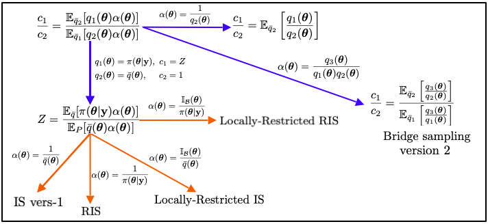
where is an arbitrary function defined on the intersection of the supports of and . Note that the expression above is an extension of the Eq. (49). Indeed, taking , we recover Eq. (49). The identity in Eq. (59) and the umbrella identity in Eq. (50) are both useful when and have little overlap, i.e., is small. Moreover, If we set , , and , then the identity becomes
| (60) |
The corresponding estimator employs samples from both and , i.e.,
| (61) |
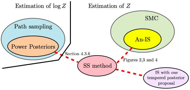
Figure 1 summarizes the connections among the Eqs. (49), (59), (60) and the corresponding different methods. The standard IS and RIS schemes have been described in the previous sections, whereas the corresponding locally-restricted versions will be introduced below.
4.2.2 Relationship with Chib’s method
The Chib estimator, described in Section 3.4, is
| (62) |
where is the proposal used inside an MCMC algorithm, represents acceptance probability of this MCMC scheme and the point is usually chosen in a high probability region. Note that the balance condition involving the function , and must be satisfied,
Using the balance condition above, if we replace inside the numerator of (62), we obtain
| (63) |
and if we also assume a symmetric proposal , we can finally write
| (64) |
We can observe a clear connection between the estimators (61) and (62). Clearly, plays the role of in (61), and the acceptance function plays the role of the function in (61). However, in this case, participates also inside the MCMC used for generating . The function takes also part to the generation MCMC chain, (being the acceptance probability of the new states), and generally its evaluation involves the evaluation of and . Note also that (62) is more generic than (64), being valid also for non-symmetric proposals . For further discussion see [36].
4.2.3 Locally-restricted IS and RIS
In the literature, there exist variants of the estimators in Eqs. (43) and (46). These corrected estimators are attempts to improve the efficiency (e.g., remove the infinite variance cases, specially in the harmonic estimator) by restricting the integration to a smaller subset of (usually chosen in high posterior/likelihood-valued regions) generally denoted by . As an example,
can be a rectangular or ellipsoidal region centered at the maximum a posteriori (MAP) estimate .
Locally-restricted IS estimator. Consider the posterior mass of subset ,
| (65) |
where is an indicator function, taking value for and otherwise. It leads to the following representation
| (66) |
We can estimate considering samples from by taking the proportion of samples inside . The resulting locally-restricted IS estimator of is
| (67) |
Note that the above estimator requires samples from two densities, namely the proposal and the posterior density (via MCMC).
Locally-restricted RIS estimator. To derive the locally-restricted RIS estimator, consider the mass of under ,
| (68) |
which leads to the following representation
| (69) |
can be estimated using a sample from by taking the proportion of sampled values inside . The locally-restricted RIS estimator is
| (70) |
Other variants, where corresponds to highest density regions, can be found in [46].
4.2.4 Optimal construction of bridge sampling
Identities as (59) are associated to the bridge sampling approach. However, considering in Eq. (59), bridge sampling can be also motivated from the expression
| (71) |
where the density is in some sense “in between” and . That is, instead of applying directly (49) to , we apply it to first estimate and , and then take the ratio to cancel . The bridge sampling estimator of is then
| (72) |
Remark 9.
We do not need to draw samples from , but only evaluate . For a comparison with umbrella sampling see Table 7.
| Method | Identity | |||
|---|---|---|---|---|
| Umbrella sampling | evaluate | draw from | evaluate | - (50) |
| Bridge sampling | draw from | evaluate | draw from | - (71) |
Optimal bridge density. It can be shown that the optimal bridge density can be expressed as a weighted harmonic mean of and (with weights being the sampling rates),
| (73) | |||||
This is an optimal bridge density if both are strictly positive, , hence we draw from both . Note that depends on the unknown ratio . Therefore, we cannot even evaluate . Hence, we need to resort to the following iterative procedure to approximate the optimal bridge sampling estimator. Noting that
| (74) |
The iterative procedure is formed by the following steps:
-
1.
Start with an initial estimate (using e.g. Laplace’s).
-
2.
For
-
(a)
Draw and and iterate
(75)
-
(a)
Remark 10.
Optimal bridge sampling for . Given the considerations above, an iterative bridge sampling estimator of is obtained by setting , , , so that
| (76) |
for . Looking at Eqs. (73) and (71), when , that is, when all samples are drawn from , the estimator above reduces to (non-iterative) standard IS scheme with proposal . When , that is, when all samples are drawn from , the estimator becomes the (non-iterative) RIS estimator. See [48] for a comparison of optimal umbrella sampling, bridge sampling and path sampling (described in the next section). An alternative derivation of the optimal bridge sampling estimator is given in [46], by generating samples from a mixture of type . However, the resulting estimator employs the same samples drawn from in the numerator and denominator, unlike in Eq. (76).
4.2.5 Other estimators drawing from a generic proposal and the posterior
Let consider again the scenario where we have a set of samples from the posterior and set from some proposal , as in the bridge sampling case described above. However, here we consider that these two sets are drawn from the mixture considering a deterministic mixture sampling approach [51], Thus, we can use the IS identities that use a single proposal, namely Eqs. (49) and (50).
Importance sampling with mixture (M-IS). Setting and in Eq. (49), we have
| (77) |
where [51]. This estimator cannot be directly used since it requires the evaluation of . From an initial guess , the following iterative procedure can be used
| (78) |
Self-IS with mixture proposal (M-Self-IS). Setting , and in Eq. (50), we have
| (79) |
where (drawn in a deterministic way). As above, this estimator is not of direct use, so we need to iterate
| (80) |
This iterative estimator is very similar to the iterative optimal bridge sampling estimator in Eq. (76), but it uses both set of samples in numerator and denominator. This estimator is also related to the reverse logistic regression method in [53] (for more details see [48, 54], and the next section). Furthermore, the iterative estimator (80) is also discussed for the case in [55], in an attempt to exploit the advantages of the Naive Monte Carlo and the harmonic mean estimators, while removing their drawbacks.
Remark 11.
4.2.6 Summary
Several techniques described in the last two subsections, including both umbrella and bridge sampling, are encompassed by the generic formula
| (81) |
as shown in Table 8. The techniques differ also for which densities are drawn from and which densities are just evaluated.
| For estimating a generic ratio | ||||||||
| Name | sampling from | |||||||
| Bridge Identity - Eq. (59) | , | |||||||
| Bridge Identity - Eq. (71) | , | |||||||
| Identity - Eq. (49) | ||||||||
| Umbrella - Eq. (50) | ||||||||
| For estimating , with one proposal | ||||||||
| Self-norm. IS - Eq. (55) | ||||||||
| IS vers-1 | ||||||||
| RIS | ||||||||
| For estimating , with two proposals, and | ||||||||
| Bridge Identity - Eq. (60) | , | |||||||
| Locally-Restricted IS | ||||||||
| Locally-Restricted RIS | ||||||||
4.3 IS based on multiple proposal densities
In this section we consider estimators of using samples drawn from more than two proposal densities. These schemes are usually based on the so-called tempering and/or annealing approach.
Reasons for tempering. The idea is again to consider densities that are in some sense “in the middle” between the posterior and an easier-to-work-with density (e.g. the prior or some other proposal density). These densities are usually scaled version of the posterior.
Generally, the scale parameter is called temperature.333The data tempering is also possible: the tempered posteriors contain less data than the complete posterior. For this reason, the resulting pdfs are usually named tempered posteriors and correspond to flatter, more diffuse distributions than the standard posterior. The use of the tempered pdfs usually improve the mixing of the MCMC algorithms and foster the exploration of the space . Generally, it helps the Monte Carlo methods (as MCMC and IS) to find the regions of posterior high probability. The number of such middle densities is specified by the user, and in some cases, it is equivalent to the selection of a temperature schedule for linking the prior and . This idea is shared by the several methods, such as path sampling, power posterior methods and stepping-stone sampling described below.
First of all, we start with a general IS scheme considering different proposals ’s. Some of them could be tempered posteriors and the generation would be performed by an MCMC method in this case.
4.3.1 Multiple Importance Sampling (MIS) estimators
Here, we consider to generate samples from different proposal densities, i.e.,
| (82) |
In this scenario, different proper importance weights can be used [51, 56, 57]. The most efficient MIS scheme considers the following weights
| (83) |
where . Indeed, considering the set of samples drawn in a deterministic order, , and given a sample uniformly chosen in , then we can write . The standard MIS estimator is
| (84) | |||||
| (85) | |||||
| (86) |
where . The estimator is unbiased [51]. As in the standard IS scheme, an alternative biased estimator is
| (87) |
where , so that and we have a convex combination of likelihood values ’s. It is a generalization of the estimator in Eq. (40) and recalled below in Eq. (88).
4.3.2 Tempered posteriors as proposal densities
Let recall the IS vers-2 estimator of in Eq. (40), which involves a weighted sum of likelihood evaluations at points drawn from importance density (but we can evaluate only ),
| (88) |
where . Let us consider
with . Namely, we use a tempered posterior as importance density. Note that we can evaluate only the unnormalized density . The IS estimator version 2 can be employed in this case, and we obtain . The resulting IS estimator version 2 is
| (89) | ||||
| (90) |
This method is denoted below as IS with a tempered posterior as proposal (IS-P). Table 9 shows that this technique includes different schemes for different values of . Different possible MIS schemes can be also considered, i.e., using Eq. (87) for instance [51, 57].
| Name | Coefficient | Weights | Estimator |
|---|---|---|---|
| Naive Monte Carlo | |||
| Harmonic Mean Estimator | |||
| Power posterior | |||
| as proposal pdf |
Remark 12.
One could consider also to draw samples from different tempered posteriors, , with , and then apply deterministic mixture idea in (87). However, in this case, we cannot evaluate properly the mixture
Here, the issue is a not just a global unknown normalizing constant (as usual): in this case, we do not know the weights of the mixture since all are unknown. This problem can be solved using the techniques described in the next sections.
Reverse logistic regression (RLR). In RLR, the idea is to apply IS with the mixture in the remark above. The normalizing constants are iteratively obtained by maximizing of a suitable log-likelihood, built with the samples from each tempered posterior [53, 58, 54].
In the next section, we describe an alternative to RLR for employing different tempered posteriors as proposals.
4.3.3 Stepping-stone (SS) sampling
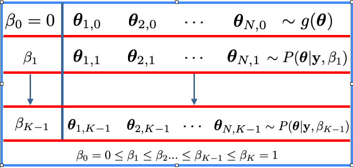
Consider again and . The goal is to estimate , which can be expressed as the following product, with and ,
| (91) |
where are often chosen as , , i.e., with a uniform grid in . Note that generally , since it is normalizing constant of the prior. The SS method is based on the following identity,
Then, the idea of SS sampling is to estimate each ratio by importance sampling as
| (92) | ||||
| (93) | ||||
| (94) |
Multiplying all ratio estimates yields the final estimator of
| (95) |
For , we come back to the Naive MC estimator. The sampling procedure of the SS method is graphically represented in Figure 2.
Remark 13.
The SS estimator is unbiased, since it a product of unbiased estimators.
The two following methods, path sampling and power posteriors, estimate instead of .
4.3.4 Path sampling (a.k.a., thermodynamic integration)
More specifically, the method of path sampling for estimating relies on the idea of building and drawing samples from a sequence of distributions linking and (a continuous path). For the purpose of estimating only one constant, the marginal likelihood , we set and and we link them by a univariate path with parameter . Let
| (96) |
denote a sequence of (probably unnormalized except for ) densities such and . More generally, we could consider where is a generic normalized proposal density, possibly closer to the posterior than . The path sampling method for estimating the marginal likelihood is based on expressing as
| (97) |
where the expectation is w.r.t. the joint , being the normalizing constant of and represents a density for . Indeed, we have
| (98) |
where we substituted and . Thus, using a sample , we can write the path sampling estimator for
| (99) |
The samples from may be obtained by first drawing () from
and then applying some MCMC steps to draw from given . Therefore, in path sampling, we have to choose (a) the path and (b) and the prior . A discussion regarding the optimal choices of the path and , see [59]. The optimal path for linking any two given densities is impractical as it depends on the normalizing constants being estimated. The geometric path described below, although suboptimal, is generic and simple to implement.
Geometric path. Often a geometric path is employed,
| (100) |
Note that is the posterior with a powered, “less informative” -“wider” likelihood (for this reason, is often called a “power posterior”). In this case, we have
so the path sampling identity becomes
| (101) |
which is also used in the power posterior method of [60], described in Section 4.3.6.
4.3.5 Connections among path sampling, bridge sampling and stepping-stones
The path sampling method can be motivated from bridge sampling by applying the bridge sampling identity in (71) in a chain fashion. Assume we have densities from which we can draw samples, with endpoints and . We can express as follows
| (102) |
Note that we have applied the bridge sampling identity in Eq. (71) to each ratio , using middle densities . We can approximate the -th term by using samples from and , and take the product to obtain the final estimator of . Taking the logarithm of the above expression, as , results in the basic identity of path sampling for estimating in Eq. (97) [59]. In this sense, path sampling can be interpreted as a continuous application of bridge sampling steps. The difference with SS method is that it employs another identity, in (92), for estimating the ratios . Figure 3 summarizes the relationships among the identities (49)-(71) and their multi-stages extensions: the SS method and path sampling scheme, respectively.
4.3.6 Method of Power Posteriors
The previous expression (101) can also be converted into an integral in as follows
| (103) |
where is a power posterior. The power posterior method aims at estimating the integral above by applying a quadrature rule. For instance, choosing a discretization , leads to approximations of order 0,
| (104) |
or order 1 (trapezoidal rule),
| (105) |
where the expected values w.r.t. the power posteriors can be independently approximated via MCMC,
| (106) |
Remark 14.
The identity (103) of method of power posteriors is derived by the path sampling identity with a geometric path, as shown in (100)-(101). In this sense, the method of power posteriors is a special case of path sampling. However, unlike in path sampling, the final approximation (105) is based on a deterministic quadrature.
Remark 15.
Remark 16.
Extensions. Several improvements of the method of power posterior have been proposed in the literature [61, 62]. In [61], the authors note that the derivative of the integrand in (103) corresponds to
| (107) |
so they propose to use this information to refine the trapezoidal rule in (105) by adding additional terms
| (108) | |||
| (109) |
This improvement comes at no extra cost since the same MCMC samples, used to estimate the expectations in (106), can be also used to estimate the variances in (109). They also propose constructing the temperature ladder recursively, starting from and , by leveraging the estimates of and (for further details see [61, Sect. 2.2]). In [62], they propose the use of control variates, a variance reduction technique, in order to improve the statistical efficiency of the estimator (105). However, this can only be applied in settings where is available.
4.3.7 On the selection of
The method of power posteriors and SS sampling require setting an increasing sequence of ’s. Some strategies for selecting the sequence of values ’s, with and , are discussed, e.g., in [60, 61, 63]. A uniform sequence for can be considered, although [60] recommends putting more values near , since it is where is changing more rapidly. More generally, we can consider . For choice of , the values are evenly-spaced quantiles of a Beta(,1), concentrating more and more near as decreases to 0 [63].
The path sampling method requires defining a prior density from which samples are drawn. It can be shown that, for any given path, the optimal choice of is a generalized local Jeffreys prior [59, Sect. 4.1].
4.3.8 Connection between stepping-stone and power posteriors methods
Taking the logarithm of the SS estimator (95), we obtain
Applying the Jensen inequality and property of the logarithm, we can write
The last expression is the estimator of the power posteriors method of order 0, i.e., replacing Eq. (106) into (104). If we denote here this estimator here as , then we have . Recall also the SS estimator is unbiased.
5 Advanced schemes combining MCMC and IS
In the previous sections, we have already introduced several methods which require the use of MCMC algorithms in order to draw from complex proposal densities. The RIS estimator, path sampling, power posteriors and the SS sampling schemes are some examples. All these previous schemes could be assigned to the family of “MCMC-within-IS” techniques. In this section, we describe more sophisticated schemes for estimating the evidence, which combine MCMC and IS techniques: Annealed Importance Sampling (An-IS) in Section 5.1, Sequential Monte Carlo (SMC) in Section 5.2, Multiple Try Metropolis (MTM) in Section 5.3, and Layered Adaptive importance Sampling (LAIS) in Section 5.4. An-IS and SMC can be also considered “MCMC-within-IS” techniques. They provide alternative ways to employ tempered posteriors and are related to SS method, described in the previous section. We also discuss the use of MCMC transitions and resampling steps for design efficient AIS schemes. The MTM algorithm described here is an MCMC method, which belongs to the family of “IS-within-MCMC” techniques. Indeed, internal IS steps are used for proposing good candidates as new state of the chain. LAIS is an AIS scheme driven by MCMC transitions. Since the the adaptation and sampling parts can be completely separated, LAIS can be considered as a “IS-after-MCMC” technique.
5.1 MCMC-within-IS: weighted samples after MCMC iterations
In this section, we will see how to properly weight samples obtained by different MCMC iterations. We denote as the transition kernel which summarizes all the steps of the employed MCMC algorithm. Note that generally cannot be evaluated. However, we can use MCMC kernels in the same fashion as proposal densities, considering the concept of the so-called proper weighting [1, 64].
5.1.1 Weighting a sample after one MCMC iteration
Let us consider the following procedure:
-
1.
Draw (where is normalized, for simplicity).
-
2.
Draw , where the kernel leaves invariant density , i.e.,
(110) -
3.
Assign to the weight
(111)
This weight is proper in the sense that can be used for building unbiased estimator (or other moments ), as described in the Liu’s definition [2, Section 14.2], [1, Section 2.5.4]. Indeed, we can write
| (112) | |||||
Note that if then , i.e., the IS weights remain unchanged after an MCMC iteration with invariant density . Hence, if we repeat the procedure above times generating , we can build the following unbiased estimator of the ,
| (113) |
In the next section, we extend this idea where different MCMC updates are applied, each one addressing a different invariant density.
5.1.2 Annealed Importance Sampling (An-IS)
In the previous section, we have considered the application of one MCMC kernel (that could be formed by different MCMC steps). Below, we consider the application of several MCMC kernels addressing different target pdfs, and show their consequence in the weighting strategy. We consider again a sequence of tempered versions of the posterior, , , , where the -th version, , coincides with the target function . One possibility is to considered or tempered posteriors,
| (114) |
as in path sampling and power posteriors. In any case, smaller values correspond to flatter distributions.444Another alternative is to use the so-called data tempering [65], for instance, setting
,
where and (recall that ).
The use of the tempered sequence of target pdfs usually improve the mixing of the algorithm and foster the exploration of the space .
Since only the last function is the true target, , different schemes have been proposed for suitable weighting the final samples.
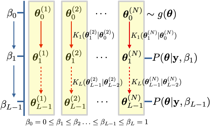
Let us consider conditional kernels (with ), representing the probability of different MCMC updates of jumping from the state to the state (note that each can summarize the application of several MCMC steps), each one leaving invariant a different tempered target, .
The Annealed Importance Sampling (An-IS) is given in Table 10.
| 1. Draw samples (usually ) for . 2. For (a) Draw leaving invariant for , i.e., we generate samples using an MCMC with invariant distribution (with different starting points ). (b) Compute the weight associated to the sample , for , (115) 3. Return the weighted sample . The estimator of the marginal likelihood is ^Z=1N∑_n=1^N ρ_L-1^(n). Combinations of An-IS with path sampling and power posterior methods can be also considered, employing the information of the rest of intermediate densities. |
Note that, when , we have . If, , then the weight is .
The method above can be modified by incorporating an additional MCMC transition , which leaves invariant . However, since is the true target pdf, as we have seen above the weight remains unchanged (see the case in the previous section). Hence, in this scenario, the output would be , i.e., . This method has been proposed in [66] but similarly schemes can be found in [65, 67].
Remark 17.
Interpretation as Standard IS.
For the sake of simplicity, here we consider reversible kernels, i.e., each kernel satisfies the detailed balance condition
| (116) |
We show that the weighting strategy suggested by An-IS can be interpreted as a standard IS weighting considering the following extended target density, defined in the extended space ,
| (117) |
Note that has the true target as a marginal pdf. Let also consider an extended proposal pdf defined as
| (118) |
The standard IS weight of an extended sample in the extended space is
| (119) |
Replacing the expression in (119), we obtain the Ann-IS weights
| (120) | |||||
| (121) |
where we have used and just rearranged the numerator. The sampling procedure in An-IS is graphically represented in Figure 4.
5.2 Weighted samples after MCMC and resampling steps
In this section, we consider also the use of resampling steps jointly with MCMC transitions. The resulting algorithm is quite sophisticated (formed by several components that should by chosen by the user) but it is a very general technique, which includes the classical particle filters, several adaptive IS (AIS) schemes and the An-IS method as special case [68].
5.2.1 Generic Sequential Monte Carlo
In this section, we describe a sequential IS scheme which encompasses the previous Ann-IS algorithm as a special case. The method described here uses jointly MCMC transitions and, additionally, resampling steps as well. It is called Sequential Monte Carlo (SMC), since we have a sequence of target pdfs , [68]. This sequence of target densities can be defined by a state-space model as in a classical particle filtering framework (truly sequential scenario, where the goal is to track dynamic parameters). Alternatively, we can also consider a static scenario as in the previous sections, i.e., the resulting algorithm is an iterative importance sampler where we consider a sequence of tempered densities , where , as in Eq.(114), so that [68]. Let us again define an extended proposal density in the domain ,
| (122) |
where is a marginal proposal and are generic forward transition pdfs, that will be used as partial proposal pdfs. Extending the space from to (increasing its dimension), note that we can write the recursive equation
The marginal proposal pdfs are
| (124) |
Therefore, we would be interested in computing the marginal IS weights, , for each . However note that, in general, the marginal proposal pdfs cannot be computed and then cannot be evaluated. A suitable alternative approach is described next. Let us consider the extended target pdf defined as
| (125) |
are arbitrary backward transition pdfs. Note that the space of increases as grows, and is always a marginal pdf of . Moreover, writing the previous equation for
and writing the ratio of both, we get
| (126) |
Therefore, the IS weights in the extended space are
| (127) | |||||
| (128) | |||||
| (129) |
where we have replaced . The recursive formula in Eq. (129) is the key expression for several sequential IS techniques. The SMC scheme summarized in Table 11 is a general framework which contains different algorithms as a special cases [68]. In Table 11, we have used the notation .
|
1.
Draw , .
2.
For
(a)
Draw samples .
(b)
Compute the weights
(130)
(131)
where we set .
(c)
Normalize the weights , for .
(d)
If :
(with and is a effective sample size measure [69], see section 5.2.2) i. Resample times according to , obtaining . ii. Set , and for all [70, 64, 71, 20]. 3. Return the cloud of weighted particles and ^Z=^Z_L=1N∑_n=1^N w_L^(n), if a proper weighting of the resampled particles is used (as suggested in the step 2(d)-ii above). Otherwise, you can use another estimator , as shown in Section 5.2.2 and the Supplementary Material. |
Choice of the forward functions.
One possible choice is to use independent proposal pdfs, i.e., or random walk proposal , where represents standard distributions (e.g., Gaussian or t-Student). An alternative is to choose , i.e., an MCMC kernel with invariant pdf .
Choice of backward functions.
It is possible to show that the optimal backward transitions are [68]
| (132) |
This choice reduces the variance of the weights [68]. However, generally, the marginal proposal in Eq. (5.2.1) cannot be computed (are not available), other possible should be considered. For instance, with the choice
| (133) |
we obtain
| (134) | |||||
| (135) |
which is exactly the update rule for the weights in An-IS.
Remark 18.
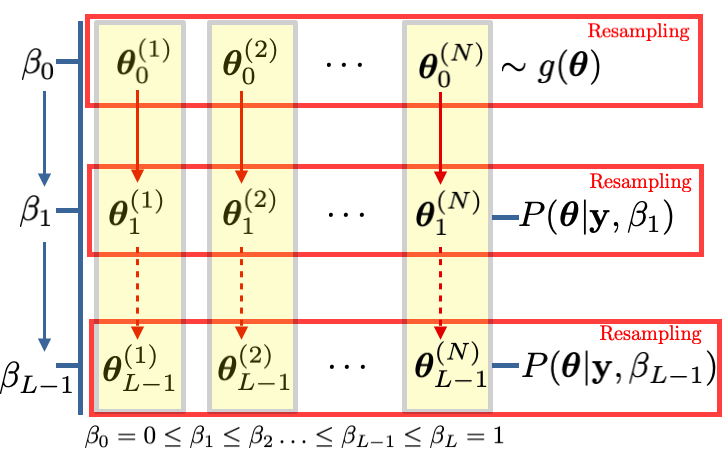
Several other methods are contained as special cases of algorithm in Table 11, with specific choice of , and , e.g., the Population Monte Carlo (PMC) method [72], that is a well-known AIS scheme. The sampling procedure in SMC is graphically represented in Figure 5.
5.2.2 Evidence computation in a sequential framework with resampling steps
The generic algorithm in Table 11 employs also resampling steps. Resampling consists in drawing particles from the current cloud according to the normalized importance weights , for . The resampling steps are applied only in certain iterations taking into account an ESS approximation, such as , or [73, 69]. Generally,if is smaller than a pre-established threshold , all the particles are resampled. Thus, the condition for the adaptive resampling can be expressed as . When , the resampling is applied at each iteration [74, 75]. If , no resampling steps are applied, and we have a simple sequential importance sampling (SIS) method. There are two possible estimators of in a sequential scenario:
| (136) |
and
| (137) |
These two estimators are equivalent in SIS (, i.e., SMC without resampling), i.e., they are the same estimator, . In SMC with and a proper weighting of the resampled particles, as used in Table 11, the two estimators are equivalent as well [70, 64, 20]. If the proper weighting of the resampled particles is not employed, is the only valid option. See Table 12 for a summary and the Supp. Material for more details.
| Scenario | Resampling | Proper Weighting [70] | Equivalence | ||
|---|---|---|---|---|---|
| SMC - (SIS) | x | — | |||
| SMC - | x | x | x | ||
| SMC - |
5.3 IS-within-MCMC: Estimation based on Multiple Try MCMC schemes
The Multiple Try Metropolis (MTM) methods are advanced MCMC algorithms which consider different candidates as possible new state of the chain [35, 76, 77]. More specifically, at each iteration different samples are generated and compared by using some proper weights. Then one of them is selected and tested as possible future state. The main advantage of these algorithms is that they foster the exploration of a larger portion of the sample space, decreasing the correlation among the states of the generated chain. Here, we consider the use of importance weights for comparing the different candidates, in order to provide also an estimation of the marginal likelihood [76].
More specifically, we consider the Independent Multiple Try Metropolis type 2 (IMTM-2) scheme [35] with an adaptive proposal pdf.
The algorithm is given in Table 13.
The mean vector and covariance matrix are adapted using the empirical estimators yielded by all the weighted candidates drawn so far, i.e., for all and . Two possible estimators of the marginal likelihood can be constructed, one based on a standard adaptive importance sampling argument [78, 79] and other based on a group importance sampling idea provided in [64].
For the sake of simplicity, we have described an independent MTM scheme, with the additional adaptation of the proposal. Random walk proposal pdfs can be also employed in an MTM algorithm [35]. In that case, the adaptation of the proposal could be not needed. However, in this scenario, the MTM algorithm requires the sampling (and weighting) of additional auxiliary points. Hence, the total number of weighted samples at each iterations are . These additional samples are just required for ensuring the ergodicity of the chain (including them in the acceptance probability ), but are not included as states of the Markov chain. But, for our purpose, they can be employed in the estimators of , as we suggest for the candidates, , in Table 13. Note that the use of a random walk proposal in an MTM scheme of type in Table 13, could be considered as “MCMC-driven IS” method, similar to the method introduced in the next section.
| 1. Choose the initial parameters , of the proposal , an initial state and a first estimation of the marginal likelihood . 2. For : (a) Draw . (b) Compute the importance weights , for . (c) Normalize them where (138) (d) Resample according to , with . (e) Set and with probability (139) otherwise set and . (f) Update computing the corresponding empirical estimators using for all and . 3. Return the chain , and . Two possible estimators of can be constructed: (140) |
5.4 IS-after-MCMC: Layered Adaptive Importance Sampling (LAIS)
The LAIS algorithm consider the use of parallel (independent or interacting) MCMC chains with invariant pdf or a tempered version [80, 78]. Each MCMC chain can address a different tempered version (or simply the posterior ) without jeopardizing the consistency of final estimators. After iterations of the MCMC schemes (upper layer), the resulting samples, , for and are used as location parameters of proposal densities . Then, these proposal pdfs are employed within a MIS scheme (lower layer), weighting the generated samples ’s with the generic weight [51, 57]. In the numerator of these weights in the lower layer, we have always the unnormalized posterior . The denominator is a mixture of (all or a subset of) proposal densities which specifies the type of MIS scheme applied [51, 57]. The algorithm, with different possible choices of , is shown in Table 14. The first choice in (142) is the most costly since we have to evaluate all the proposal pdfs in all the generated samples ’s, but provides the best performance in terms of efficiency of the final estimator. The second and third choices are temporal and spatial mixtures, respectively. The last choice corresponds to standard importance weights given in Section 4.
| 1. Generate samples, , using parallel MCMC chains of length , each MCMC method using a proposal pdf , with invariant distributions a power posterior (with ) or a posterior pdf with a smaller number of data. 2. Draw samples where plays the role of the mean, and is a covariance matrix. 3. Assign to the weights (141) There are different possible choices for , for instance: (142) (143) (144) (145) 4. Return all the pairs , and . |
Let assume for all in the upper layer. Considering also standard parallel Metropolis-Hastings chains in the upper layer, the number of posterior evaluations in LAIS is . Thus, if only one chain is employed in the upper layer, the number of posterior evaluations is .
Special case with recycling samples. The method in [81] can be considered as a special case of LAIS when , and i.e., all the samples are generated by the unique MCMC chain with random walk proposal with invariant density . In this scenario, the two layers of LAIS are collapsed in a unique layer, so that . Namely, no additional generation of samples are needed in the lower layer, and the samples generated in the upper layer (via MCMC) are recycled. Hence, the number of posterior evaluations is only . The denominator for weights used in [81] is in Eq. (143), i.e., a temporal mixture as in [82]. The resulting estimator is
Relationship with KDE method. LAIS can be interpreted as an extension of the KDE method in Section 3, where the KDE function is also employed as a proposal density in the MIS scheme. Namely, the points used in Eq. (26), in LAIS they are drawn from the KDE function using the deterministic mixture procedure [51, 56, 57].
Compressed LAIS (CLAIS). Let us consider the or is large (i.e., either large chains or several parallel chains; or both). Since is large, the computation of the denominators Eqs. (142)- (143)- (144) can be expensive. A possible solution is to use a partitioning or clustering procedure [83] with clusters considering the samples, and then employ as denominator the function
| (146) |
where represents the centroid of the -th cluster, the normalized weight is proportional to the number of elements in the -th cluster (), and with the empirical covariance matrix of -th cluster and .
Relationship with other methods using tempered posteriors. In the upper layer of LAIS, we can use non-tempered versions of the posterior, i.e., for all , or tempered versions of the posterior . However, unlike in SS and/or power posterior methods, these samples are employed only as location parameters of the proposal pdfs , and they are not included in the final estimators. Combining the tempered posteriors idea and the approach in [81], we could recycle and use where we denote as the proposal pdfs employed in the MCMC chains. Another difference is that, in LAIS, the use of an “anti-tempered” posteriors with is allowed and can be shown that is beneficial for the performance of the estimators (after the chains reach a good mixing) [84]. More generally, one can consider a time-varying (where is the iteration of the -th chain). In the first iterations, one could use for fostering the exploration of the state space and helping the mixing of the chain. Then, in the last iterations, one could use which increases the efficiency of the resulting IS estimators [84].
6 Vertical likelihood representations
In this section, we introduce a different approach based on Lebesgue representations of the integral expressing the marginal likelihood . First of all, we derive two one-dimensional integral representations of , and then we describe how it is possible to use these alternative representations by applying one-dimensional quadratures. However, the application of these quadrature rules is not straightforward. A possible final solution is the so-called nested sampling method.
6.1 Lebesgue representations of the marginal likelihood
6.1.1 First one-dimensional representation
The -dimensional integral can be turned into a one-dimensional integral using an extended space representation. Namely, we can write
| (147) | ||||
| (148) | ||||
| (149) |
where is an indicator function which is if and otherwise. Switching the integration order, we obtain
| (150) | ||||
| (151) | ||||
| (152) |
where we have set
| (153) |
In Eq. (152), we have also assumed that is bounded so the limit of integration is .
Below, we define several variables and sampling procedures required for the proper understanding of the nested sampling algorithm.
6.1.2 The survival function and related sampling procedures
The function above is the mass of the prior restricted to the set . Note also that
| (154) |
Moreover, we have that with and for all , and it is also an non-increasing function. Therefore, is a survival function, i.e.,
| (155) |
is the cumulative distribution of the random variable with [85, 2].
Sampling according to . Since with , the following procedure generates samples from :
-
1.
Draw , for .
-
2.
Set , , for all .
Recalling the inversion method [85, Chapter 2], note also that the corresponding values
| (156) |
i.e., they are uniformly distributed in . Since , and since is also uniformly distributed if , then
| (157) |
In summary, finally we have that
| (158) |
6.1.3 The truncated prior pdf and other sampling procedures
Note that is also the normalizing constant of the following truncated prior pdf
| (159) |
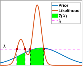
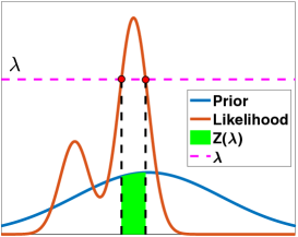
where and for . Two graphical examples of and are given in Figure 7.
Sampling from and . Given a fixed value , in order to generate samples from one alternative is to use an MCMC procedure. However, in this case, the following acceptance-rejection procedure can be also employed [85]:
-
1.
For :
-
(a)
Draw .
-
(b)
if then set and .
-
(c)
if , then reject and repeat from step 1(a).
-
(a)
-
2.
Return and .
Observe that , for all , and the probability of accepting a generated sample is exactly . The values where , have the following truncated cumulative distribution
| (160) |
i.e., we can write .
6.1.4 Distribution of and if
6.1.5 Distributions
Let us consider and the minimum and maximum values
| (162) |
Let us recall . Then, note that is maximum of uniform random variables
Then it is well-known that the cumulative distribution of the maximum value
is distributed according to a Beta distribution , i.e., and density [85, Section 2.3.6]. In summary, we have
| (163) |
This result is important for deriving the standard version of the nested sampling method, described in the next section. A summary of the relationships presented above is provided in Table 15.
6.1.6 Second one-dimensional representation
Now let consider a specific area value . The inverse function
| (164) |
is also non-increasing. Note that if and only if . Then, we can write
| (165) |
6.1.7 Summary of the one-dimensional representations
Thus, finally we have obtained two one-dimensional integrals for expressing the Bayesian evidence ,
| (166) |
Now that we have expressed the quantity as an integral of a function over , we could think of applying simple quadrature: choose a grid of points in () or in (), evaluate or and use the quadrature formulas
| (167) | ||||
| (168) |
However, this simple approach is not desirable since (i) the functions and are intractable in most cases and (ii) they change much more rapidly over their domains than does , hence the quadrature approximation can have very bad performance, unless the grid of points is chosen with extreme care. Table 16 summarizes the one-dimensional expression for and contained in this work. Clearly, in all of them, the integrand function depends, explicitly or implicitly, on the variable .
6.2 Nested Sampling
Nested sampling is a technique for estimating the marginal likelihood that exploits the second identity in (166) [28, 86, 26]. Nested Sampling estimates by a quadrature using nodes (in decreasing order),
and the quadrature formula
| (169) |
with . We have to specify the grid points ’s (possibly well-located, with a suitable strategy) and the corresponding values . Recall that the function , and its inverse , are generally intractable, so that it is not even possible to evaluate at a grid of chosen ’s.
Remark 19.
The nested sampling algorithm works in the other way around: it suitably selects the ordinates ’s and find some approximations ’s of the corresponding values . This is possible since the distribution of is known (see Section 6.1.5).
6.2.1 Choice of and in nested sampling
Nested sampling employs an iterative procedure in order to generate an increasing sequence of likelihood ordinates , , such that
| (170) |
The details of the algorithm is given in Table 17 and it is based on the sampling of the truncated prior pdf (see Sections from 6.1.2 to 6.1.5), where denotes the iteration index. The nested sampling procedure is explained below:
-
•
At the first iteration (), we set and . Then, samples are drawn from the prior obtaining a cloud and then set , i.e., as shown in Section 6.1.2. Thus, the first ordinate is chosen as
Since , using the result in Eq. (163), we have that
Since , then . The corresponding is also removed from , i.e., (now ).
-
•
At a generic -th iteration (), a unique additional sample is drawn from the truncated prior and added to the current cloud of samples, i.e., (now again ). First of all, note that the value is distributed as (see Section 6.1.3). More precisely, note that all the ordinate values
are distributed as , i.e., . This is due to how the population has been built in the previous iterations. Then, we choose the new minimum value as
Moreover, since is the minimum value of , in Section 6.1.5 we have seen that
(171) where we have used Eq. (163). We remove again the corresponding sample , i.e., we set and the procedure is repeated. Note that we have also found the recursion among the following random variables,
(172) for and .
-
•
The random value could be estimated and replaced with the expected value of the Beta distribution , i.e.,
(173) where , and becomes a very good approximation as grows. In that case, the recursion above becomes
(174) Then, denoting , we can use as an approximation of .
Remark 20.
The intuition behind the iterative approach above is to accumulate more ordinates close to the . They are also more dense around . Moreover, using this scheme, we can employ as an approximation of .
Remark 21.
An implicit optimization of the likelihood function is performed in the nested sampling algorithm. All population of approaches the value .
| 1. Choose and set . 2. Draw and define the set . Let us also define the notation (175) 3. Set and . 4. Set , i.e., eliminate from . 5. Find an approximation of . One usual choice is . 6. For (a) Draw and add to the current cloud of samples, i.e., . (b) Set and . (c) Set . (d) Find an approximation of . One usual choice is (176) The rationale behind this choice is explained in the section above. 7. Return (177) |
6.2.2 Further considerations
Perhaps, the most critical task of the nested sampling implementation consists in drawing from the truncated priors. For this purpose, one can use a rejection sampling or an MCMC scheme. In the first case, we sample from the prior and then accept only the samples such that . However, as grows, its performance deteriorates since the acceptance probability gets smaller and smaller. The MCMC algorithms could also have poor performance due to the sample correlation, specially when the support of the constrained prior is formed by disjoint regions or distant modes [86]. Moreover, in the derivation of the standard nested sampling method we have considered different approximations. First of all, for each likelihood value , its corresponding is approximated by replacing the expected value of a Beta random variable within a recursion involving (Eq. (172)). Then this expected value is again approximated with an exponential function in Eq. (173). This step could be avoided, keeping directly . The simplicity of the final formula is perhaps the reason of using the approximation . A further approximation is also implicitly applied in (174). Additionally, if an MCMC method is run for sampling from the constrained prior, also the likelihood values are in some sense approximated due to the possible burn-in period of the chain.
6.2.3 Generalized Importance Sampling based on vertical representations
Let us recall the estimator IS vers-2 with proposal density ,
| (178) |
where and . In [26], the authors consider the use of the following proposal pdf
| (179) |
where the function is defined by the user. Using leads to the weights of the form
| (180) |
Note that choosing we have , and , recovering the harmonic mean estimator. With , we have and , recovering the method in Section 4.3.2 that uses a power posterior as a proposal pdf. Nested sampling seems that can be also included in this framework [26].
7 On the marginal likelihood approach and other strategies
In this section, we examine the marginal likelihood approach to Bayesian model selection and compare it to other strategies such as the well-known posterior predictive check approach.
7.1 Dependence on the prior and related discussion
The marginal likelihood approach for model selection and hypothesis testing naturally appears as a consequence of the application of Bayes’ theorem to derive posterior model probabilities . Under the assumption that one of is the true generating model, the Bayes factor will choose the correct model as the number of data grows, [87]. We can also apply the posterior model probabilities to combine inferences across models, a setting called Bayesian model averaging [19, 20].
7.1.1 Dependence on the prior
In Section 2.2, we have seen the marginal likelihood contains intrinsically a penalization for the model complexity. This penalization is related to the choice of the prior and its “overlap” with likelihood function. Indeed, is by definition a continuous mixture of the likelihood values weighted according to the prior. In this sense, depending on the choice of the prior, the evidence can take any possible value in the interval (see Section 2.2, for more details). Hence, the marginal likelihood even with strong data (unlike the posterior density) is highly sensitivity to the choice of prior density. See also the examples in the Supplementary Material.
Improper priors. The use of improper priors, , is allowed when , since the corresponding posteriors are proper.
However, this is an issue for the model selection with . Indeed,
the prior is not completely specified, since is arbitrary. Some possible solutions are given in Section 7.2.
Generally, the use of more diffuse (proper) priors provides smaller values of . Therefore, different choices of the priors can yield different selected models. For this fact, some authors criticize the use of evidence for model comparison.
7.1.2 Safe scenarios for fair comparisons
In a Bayesian framework, the best scenario is clearly when the practitioners and/or researchers have strong beliefs that can be translated into informative priors. Hence, in this setting, the priors truly encode some relevant information about the inference problem.
When this additional information is not available, different strategies could be considered. We consider as a safe scenario for comparing different models, a scenario where the choice of the priors is virtually not favoring any of the models.
Below and in Sections 7.2 and 7.4, we describe some interesting scenarios and some possible solutions for reducing, in some way, the dependence of the model comparison on the choice of the priors.
Same priors. Generally, we are interested in comparing two or more models. The use of the same (even improper) priors is possible when the models have the same parameters (and hence also share the same support space). With this choice, the resulting comparison seems fair and reasonable. However, this scenario is very restricted in practice.
An example is when we have nested models. As noted in [87, Sect. 5.3], in the context of testing hypothesis, some authors have considered improper priors on nuisance parameters that appear on both null and alternative hypothesis. Since the nuisance parameters appear on both models, the multiplicative constants cancel out in the Bayes factor.
Likelihood-based priors. When , we can build a prior based on the data and the observation model. For instance, we can choose , then the marginal likelihood is
| (181) |
This idea is connected to posterior predictive approach, described in Section 7.4. Indeed, the marginal likelihood above can be written as when . Less informative likelihood-based priors can be constructed using a tempering effect with a parameter or considering only a subset of data . For instance, when or , then we can choose or , the marginal likelihood is
| (182) |
This is also the key idea underlying the partial and intrinsic Bayes factors described in the next section.
7.2 Bayes factors with improper priors
So far we have considered proper priors, i.e., . The use of improper priors is common in Bayesian inference to represent weak prior information. Consider where is a non-negative function whose integral over the state space does not converge, . In that case, is not completely specified. Indeed, we can have different definitions where is (the inverse of) the “normalizing” constant, not uniquely determinate since formally does not exist. Regarding the parameter inference and posterior definition, the use of improper priors poses no problems as long as , indeed
| (183) |
where , and . Note that the unspecified constant is canceled out, so that the posterior is well-defined even with an improper prior if . However, the issue is not solved when we compare different models, since depends on . For instance, the Bayes factors depend on the undetermined constants [88],
| (184) |
so that different choices of provide different preferable models.
There exists various approaches for dealing with this issue. Below we describe some relevant ones.
Partial Bayes Factors. The idea behind the partial Bayes factors consists of using a subset of data to build proper priors and, jointly with the remaining data, they are used to calculate the Bayes factors. This is related to the likelihood-based prior approach, described above.
The method starts by dividing the data in two subsets, . The first subset is used to obtain partial posterior distributions,
| (185) |
using the improper priors. The partial posterior is then employed as prior. Note that
Recall that the complete posterior of -th model is
| (186) |
where
Note that and both depend on the unspecified constant . Considering the conditional likelihood of the remaining data ,555In case of conditional independence of the data given , we have . we can study another posterior of ,
| (187) |
where in (185) plays the role of a prior pdf, and
Thus, does not depend on . Therefore, considering the partial posteriors as proper priors, we can define the following partial Bayes factor
| (188) |
Therefore, one can approximate firstly , secondly and then compare the model using the partial Bayes factor .
Remark 22.
The trick here consists in computing two normalizing constants for each model, instead of only one. The first normalizing constant is used for building an auxiliary proper prior, depending on . The difference with the likelihood-based prior approach in previous section is that is used only once (in the auxiliary proper prior).
A training dataset is proper if for all models, and it is called minimal if is proper and no subset of is proper. If we use actually proper prior densities, the minimal training dataset is the empty set and the fractional Bayes factor reduces to the classical Bayes factor. However, the main drawback of the partial Bayes factor approach is the dependence on the choice of (which could affect the selection of the model). The authors suggest finding the minimal suitable training set , but this task is not straightforward. Two alternatives in the literature have been proposed, the fractional Bayes factors and the intrinsic Bayes factors.
Fractional Bayes Factors [89]. Instead of using a training data, it is possible to use power posteriors, i.e.,
| (189) |
where the denominator is
| (190) |
with , and . Note that the value is not admissible since for .
Again, since both and depend on the ratio , the fractional Bayes factor is independent on and by definition.
Intrinsic Bayes factors [90]. The partial Bayes factor (7.2) will depend on the choice of (minimal) training set . These authors solve the problem of choosing the training sample by averaging the partial Bayes factor over all possible minimal training sets. They suggest using the arithmetic mean, leading to the arithmetic intrinsic Bayes factor, or the geometric mean, leading to the geometric intrinsic Bayes factor.
7.3 Marginal likelihood as a prior predictive approach
Due to the definition of the marginal likelihood is also called or related to the so-called prior predictive approach. As in the Approximate Bayesian Computation (ABC) [91], the idea is that we can generate artificial data , from each -th model with the following procedure: (a) draw from the -th prior, and from the -th likelihood . Given each set of fake data , we can use different classical hypothesis testing techniques for finding the set closest to the true data (for instance, based on -values). Another possibility, we could approximate the value applying kernel density estimation to each set .
In the next section, we describe the posterior predictive approach, which consider the expected value of likelihood evaluated in a generic with respect to (w.r.t.) the posterior , instead of w.r.t. the prior . The posterior predictive idea can be considered an alternative model selection approach w.r.t. the marginal likelihood approach, which includes several well-known model selection schemes.
7.4 Other ways of model selection: the posterior predictive approach
The marginal likelihood approach is not the unique approach for model selection in Bayesian statistics. Here, we discuss some alternatives which are based on the concept of prediction.
After fitting a Bayesian model, a popular approach for model checking (i.e. assessing the adequacy of the model fit to the data) consists in measuring its predictive accuracy [92, Chapter 6][93].
Hence, a key quantity in these approaches is the posterior predictive distribution of generic different data given ,
| (191) |
Considering , note that exists a clear connection with likelihood-based priors described in Section 7.1.
Remark 23.
The posterior predictive distribution in (191) is an expectation w.r.t. the posterior, which is robust to the prior selection with informative data, unlike the marginal likelihood. Therefore, this approach is less affected by the prior choice.
Note that we can consider posterior predictive distributions for vectors smaller than (i.e., with less components).
The posterior predictive checking is based on the main idea of considering some simulated data , with , and comparing with the observed data . After obtaining a set of fake data , we have to measure the discrepancy between the true observed data and the set . This comparison can be made with test quantities and graphical checks (e.g., posterior predictive p-values).
Alternatively, different measures of predictive accuracy can be employed. An example, is the expected log pointwise predictive density (ELPD) [94]. Let recall that , and define as any alternative scalar data. Considering alternative scalar data with density , the ELPD is defined as
| ELPD | ||||
| (192) |
Note that is the density representing the true data generating process for , which is clearly unknown. Therefore, some approximations are required. First all, we define an over-estimation of the ELPD, considering the observed data in instead new alternative data , so that and , i.e.,
| (193) |
In practice, we need an additional approximation for computing . We can use MCMC samples from , i.e.,
| (194) |
LOO-CV. However, we know that the approximation above overestimates ELPD. One possibility is to use cross-validation (CV), such as the leave-one-out cross-validation (LOO-CV). In LOO-CV, we consider instead of in Eq. (193), where is vector leaving out the -th data, . Hence,
| (195) |
For approximating , we draw again from the full posterior by means of an MCMC technique, , and apply importance sampling [94],
| (196) |
where and, in the case the data are conditionally independent,
Thus, replacing in (196), we obtain
| (197) |
which resembles the harmonic mean estimator but with just one data point. However, since the full posterior has smaller variance of , the direct use of (197) is quite unstable, since the IS weights can have high or infinite variance. See [94] for stable computations of LOO-CV and using posterior simulations. Moreover, see also [93] for a quantitative comparison of methods for estimating the predictive ability of a model. The marginal likelihood can also be interpreted as a measure of predictive performance [87, Sect. 3.2]. In [95], the authors show that the marginal likelihood is equivalent, in some sense, to a leave-p-out cross-validation procedure. For further discussions about model selection strategies, see [96, 97].
8 Numerical comparisons
In this section, we compare the performance of different marginal likelihood estimators in different experiments. First of all, we consider 3 different illustrative scenarios in Section 8.1, 8.2 and 8.3 each one considering different challenges: different overlap between prior and likelihood (changing the number of data, or the variance and mean of the prior), multi-modality and different dimensions of the inference problem. The first experiment also considers two different sub-scenarios. Additional theoretical results related to the experiments in Sect. 8.1 are provided in the Supplementary Material.
The last two experiments involves a real data analysis. In Section 8.4, we test several estimators in a nonlinear regression problem with real data (studied also in [30]), where the likelihood function has non-elliptical contours. Finally, in Section 8.5 we consider another regression problem employing non-linear localized bases with real data of the COVID-19 outbreak.
8.1 First experiment
8.1.1 First setting: Gaussians with same mean and different variances
In this example, our goal is to compare by numerical simulations different schemes for estimating the normalizing constant of a Gaussian target . We know the ground-truth , so .
Since this is a data-independent example, and have no dependence on . We compare several estimators enumerated below, considering one or two proposals.
One proposal estimators (IS and RIS). First of all, we recall that the IS vers-1 estimator with importance density and the RIS estimator with auxiliary density are
For a fair comparison, we consider
where is the standard deviation. We desire to study the performance of the two estimators as varies. Moreover, a theoretical comparison of IS and RIS estimators is given in the Supplementary Material.
Estimators using with two proposals. The IS and RIS estimators use a single set of samples from or , respectively. Now, we consider the comparison, in terms of MSE, against several estimators that use sets of samples from both densities, and , at the same time. Let and denote sets of iid samples from and , respectively. When , the set can be considered as a unique set of samples drawn from the mixture [51]. For a fair comparison, these estimators use samples from and samples from .
Ideal and realistic scenarios. Furthermore, we consider two scenarios, corresponding to whether we can evaluate (ideal and impossible scenario) or we evaluate (realistic scenario). Note that the first scenario is simply for illustration purposes.
Jointly with IS and RIS estimator, we test several other estimators of , introduced in Section 4.2, that use two sets of samples simultaneously.
-
•
Opt-BS: The optimal bridge sampling estimator with .
-
•
Mix-IS: IS vers-1 with the mixture , instead of , as proposal.
-
•
Mix-self IS: The self-IS estimator, with , and the mixture as the proposal.
Moreover, we consider another one proposal estimator, described in Section 4.1.3:
-
•
Opt-self IS: The optimal self-IS estimator, with . Note that this estimator use samples from a density to . We include it as a reference, for its optimality, and since involves both, and .
Remark 24.
Clearly, in the realistic scenario, all of the schemes above must replaced for their iterative versions, since we cannot evaluate but only .
Results in ideal scenario. Figures 8(a)-(b) show the MSE of the estimators versus (which is the standard deviation of ) in the ideal scenario.
IS vers-1 can have very high MSE when , i.e., has smaller variance then the .
Whereas, IS vers-1 is quite robust when .
The MSE of RIS has the opposite behavior of IS vers-1. This is because RIS needs that has lighter tails than .
In this example, optimal bridge sampling seems to provide performance in-between the IS and RIS estimators. The MSE of Opt-BS is closer to RIS for , whereas Opt-BS becomes closer to IS for . Conversely, the MSE of Opt BS is not smaller than that of IS or RIS for any in this example. Finally, Mix-IS and Mix-self-IS provide the best performance, even better than the optimal self-IS estimator. But this is due to we are in an ideal, unrealistic scenario.
Results in the realistic scenario. Since is unknown we cannot evaluate but only . Only IS and RIS can be truly applied. The rest of above estimators must employ an iterative procedure (see Section 4.1.3 and Section 4.2).
The iterative versions of these estimators evaluate , where is the current approximation.
In Figure 9, we show these three estimators after and iterations.
Interestingly, note that they all converge to the results of Opt-BS estimator. This means that the iterative versions of Mix-IS and Mix-self-IS are two alternative of Opt-BS in practice, and the performance obtained in ideal scenario are unachievable. However, the iterative version of Opt-BS seems to have the fastest convergence (to the results of the ideal Opt-BS), w.r.t. the iterative versions of Mix-IS and Mix-self-IS.
We also include a two-stage version of the Opt-selfIS estimator (see Section 4.1.2). This estimator employs to obtain an approximation via standard IS, and then draws samples from a density proportional to . This two-stage Opt-selfIS depends on the quality of the initial approximation of . Since this initial approximation is provided by IS, and since IS is problematic when , the two-stage self-IS does not perform better than Opt-BS for .
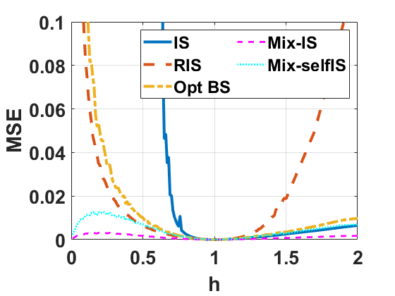
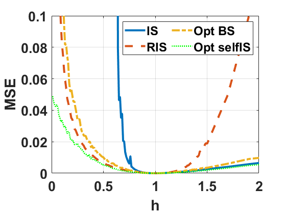
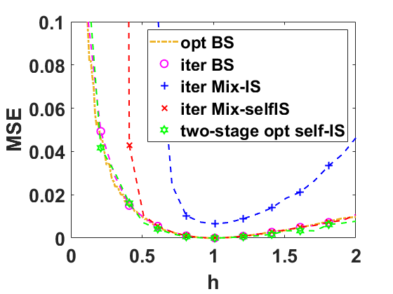
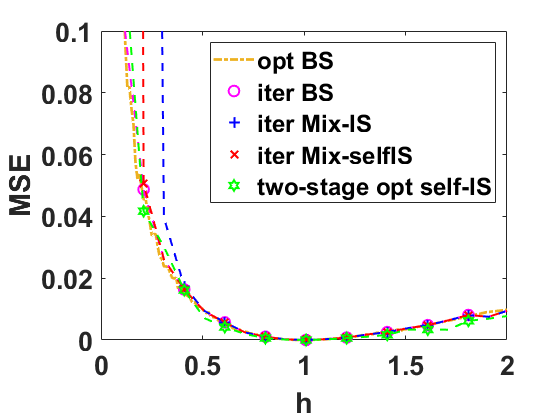
8.1.2 Second setting: Gaussians with same variance and different means
In this setting, we consider again ,i.e., , but the proposal is for . Namely, as grows, and are more distant. A theoretical comparison of IS and RIS estimators is given in the Supplementary Material, also for this setting.
Similarly, we compare the MSE as function of of different estimators of : (a) IS vers-1, (b) RIS, (c) optimal BS (Opt-BS), (d) a suboptimal self-IS estimator with and using as proposal,
and (e) the Opt-self IS estimator with and proposal . Each estimator is computed using samples in total and the results are averaged over 2000 independent simulations.
Results of the second setting. Unlike in the first setting, here we consider only the ideal scenario (i.e., without iterative procedures). However, note that the suboptimal self-IS scheme would not require an iterative version.
The results are shown in Figure 10. The MSE of both IS and RIS diverge as .
Opt-BS shows better performance than IS vers-1 and RIS.
The suboptimal self-IS estimator performs similarly to the Opt-BS, but both are worse than the Opt-self IS estimator. In this example, the estimators that use a middle density (as Opt-BS and the self-IS estimators) are less affected by the problem of and becoming further apart.
As in the previous setting, we expect that the iterative versions of Opt-BS converges to the results of the ideal Opt-BS, provided in Figure 10.
Recall that, for approximating the Opt-self IS, we require a two-stage procedure. However, a procedure with just two stages could be not enough, as we showed in the previous setting. Hence, an iterative application of the two-stage procedure could be employed (becoming actually an adaptive importance sampler).
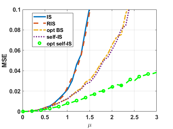
8.2 Second experiment: Gaussian likelihood and uniform prior
Let us consider the following one-dimensional example. More specifically, we consider independent data generated according to a Gaussian observation model,
where , and denote the sample mean and sample variance of , respectively. We consider a uniform prior with being the prior width. In this setting, the marginal likelihood can be obtained in closed-form as a function of and (considering the evaluation of the error function ). The posterior is a truncated Gaussian . Let denote an inverse temperature, the power posterior is
| (198) |
For any , we can sample
with rejection sampling by drawing from and discarding the samples that fall outside .
Scenario 1: and . We start by setting and generating data points from with .
The value of the marginal likelihood is .
We aim to compare the performances of several methods in estimating :
(a) Naive Monte Carlo (NMC), (b) Harmonic mean (HM), (c) IS with a tempered posterior as proposal (IS-P),
(d) stepping stone sampling (SS), (e) power posterior method (PP), and (f) path sampling (PS).
Remark 25.
Estimating , instead of directly , helps the methods of PP and PS, with respect to NMC, HM, IS-P and SS (making their results worse).
We establish a total budget of likelihood evaluations.
For SS and PP, we set values of , from to , chosen (i) uniformly, i.e., for , or (ii) concentrated around , i.e., with .
Hence the uniform case is obtained when .
Note that SS draws samples from distributions, while PP draw samples from distributions.
For fair comparison, we sample times from each , for , in SS, and times from of each , for , in PP. For IS-P we test and and draw samples from each of the and . For PS, we sample pairs as follows: we first sample from a and then sample from the corresponding power posterior . Naive Monte Carlo uses independent samples from prior and HM uses independent samples from the posterior.
Results scenario 1. In Figure 11(a), we show 500 independent estimations from each method. We observe that NMC works very well in this scenario since the prior acts as a good proposal. SS with provides also good performance, since half the samples come from the prior with this choice of . The value of seems to be not important for SS in this case.
PS performs as well as NMC and SS, but shows a slightly bigger dispersion. HM tends to overestimate the marginal likelihood, which is a well-known issue.
The estimation provided by IS-P depends on the choice of . For , the power posterior is closer to the posterior so its behavior is similar to HM. For the power posterior is close to the prior, and IS-P tends to underestimate . Recall that IS-P has a bias since it is a special case of IS vers-2. PP performs poorly with , due to the discretization error in (103), which improves when considering the value . The choice , w.r.t. , improves the performance in PP.
In Figure 11(b), we show the mean absolute error (MAE) in estimating of SS and PP as a function of . We depict two curves for each method, corresponding to the choices and . We can observe that the errors obtained in SS and PP when are smaller than when for any . This is in line with the recommendations provided in their original works. We note that the error of SS slightly deteriorates as grows: for , less and less samples are drawn from the prior, which is a good proposal in this scenario (with and ). The performance of PP improves drastically as grows, since larger means that the trapezoidal rule is more accurate in approximating (103). SS and PP, for and , approach the same limit when grows, achieving an error which is always greater than the one obtained by NMC, in this scenario.
Scenario 2: and . Now, we replicate the previous experiment increasing the number of data, , and the width of the prior, . The joint effect of increasing and makes the likelihood become extremely concentrated w.r.t. the prior, hence decreasing the value of the marginal likelihood, being .
Moreover, this high discrepancy between prior and posterior is reflected in the power posteriors , which will be very similar to the posterior except for very small values of .
We compare all the methods described before with a total budget of likelihood evaluations. Additionally, we also test a PS where , i.e., from a beta distribution which provides more values closer to .
Results scenario 2. In Figure 12(a), we can see that, unlike in the previous scenario, the NMC tends to underestimate the marginal likelihood, since the likelihood is much more concentrated than the prior.
The HM and the two implementations of IS-P provide similar results, overestimating : in this case, the posterior is so different from the prior that and are very similar to the posterior.
PS with tends to overestimate : since the ’s are drawn uniformly in , many samples are drawn in high-valued likelihood zones. Indeed, at least the bias is reduced when we test PS with . We also show the results of one implementation of SS (with and ) and PP (with and ). Both greatly outperform the rest of estimators in this scenario, providing accurate estimations. In Figure 12(b), we show again the MAE of SS and PP as a function of for two values and . The error of PP, with either or , decreases as grows, although it decreases more rapidly when considering . The error of SS with decreases as grows, but increases with when . Again, PP requires the use bigger values of with respect to SS. In both methods, the choice of , i.e., concentrating ’s near where is usually changing rapidly, shows to improve the overall performance.
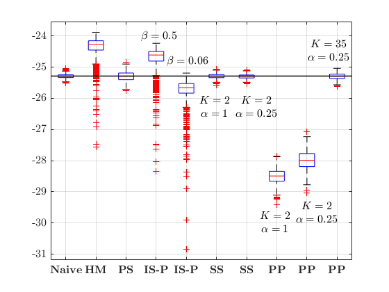
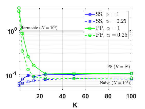
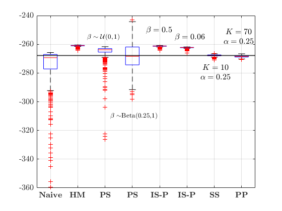
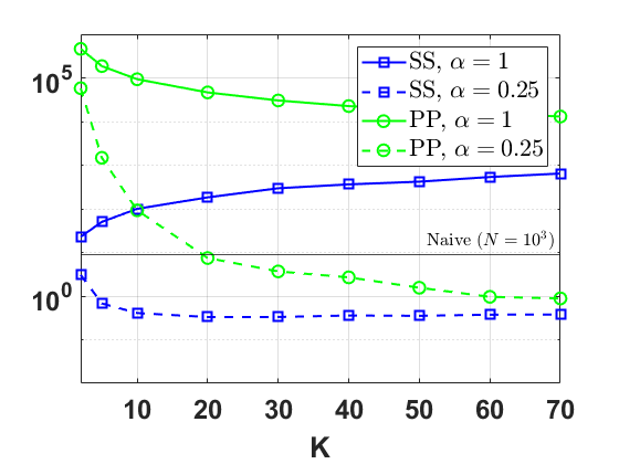
8.3 Third experiment: posterior as mixture of two components
We consider a posterior which is a mixture of two -dimensional Gaussian densities. It is a conjugate model where the likelihood is Gaussian and the prior is a mixture of two Gaussian. Given the observation vector , we consider a -dimensional Gaussian likelihood function
| (199) |
with covariance , and a -dimensional Gaussian mixture prior
| (200) |
with , and being the prior means and covariances of each component of the mixture, respectively. Then, the posterior is also a mixture of two Gaussian densities
| (201) |
where the parameters , and can be obtained in closed-form from , , , and . Thus, having the analytical expression of the posterior in closed-form allows to compute exactly the marginal likelihood (recall for any ). In this case, we can also draw samples directly from the posterior. We can interpret this scenario as the use of an ideal MCMC scenario, where the performance is extremely good. We compare different estimators of changing the Euclidean distance between the means of posterior mixture components,
| (202) |
in and . This distance can be controlled by changing the distance between the prior modes. More specifically, we choose , , where denotes the -dimensional identity matrix. The data is a single observation , where a -dimensional vector of ’s. For the prior means we chose , so . We can change the distance between the modes of the prior, and hence between the modes of the posterior, by varying . Specifically, we select and compare: (i) the Naive-MC estimator, (ii) the HM estimator, (iii) Laplace-Metropolis estimator, (iv) RIS, and (v) CLAIS. The budget is posterior evaluations. In RIS, we set to be the mixture in Eq. (146), that results after applying a clustering algorithm (e.g., k-means algorithm) to the posterior samples. In CLAIS, we use an analogous mixture obtained from posterior samples, and then use it to draw other samples in the lower layer (hence the total number of posterior evaluations is ). For RIS and CLAIS, we set the number of clusters to . RIS and CLAIS also need setting the bandwidth parameter (see Eq. (146)). We find that the choices for RIS and for CLAIS show the average performance of both. We test the techniques in dimension and . We compute the relative Mean Absolute Error (MAE) in the estimation of , averaged over independent simulations.
The results are depicted in Figure 13. They show that RIS and the CLAIS achieve the best overall performances. Their relative error remain small and rather constant for all distances considered, for and . The RIS estimator performs as well as CLAIS in both and , and even better for small distances in . For the smallest distance, the lowest relative error corresponds to the Naive MC estimator, since prior and posterior are very similar in that case, although it rapidly gets outperformed by RIS and CLAIS. The Laplace estimator provides poor results as dist grows, since the posterior becomes bimodal. As one could expect, the estimators that make use of the posterior sample to adapt its importance density, i.e., RIS and CLAIS, achieve best performances, being almost independent to increasing the distance between the modes. The HM estimator confirms its reputation of relative bad estimator.
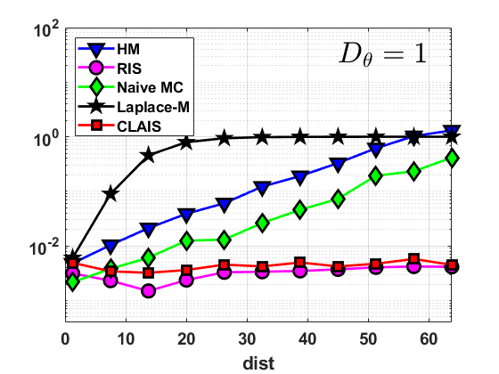
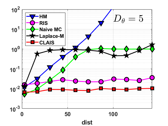
8.4 Experiment with biochemical oxygen demand data
We consider a numerical experiment studied also in [30], that is a nonlinear regression problem modeling data on the biochemical oxygen demand (BOD) in terms of time instants. The outcome variable (mg/L) is modeled in terms of (days) as
| (203) |
where the ’s are independent errors, hence . The data , measured at locations , are shown in Table 18 below.
| (days) | (mg/L) |
|---|---|
| 1 | 8.3 |
| 2 | 10.3 |
| 3 | 19.0 |
| 4 | 16.0 |
| 5 | 15.6 |
| 7 | 19.8 |
The goal is to compute the normalizing constant of the posterior of given the data . Following [30], we consider uniform priors for , and , i.e., for , and , with . Moreover, we consider an improper prior for , . However, we will integrate out the variable . Indeed, the two-dimensional target results after integrating out by marginalizing
w.r.t. , namely we obtain
| (204) | ||||
| (205) |
for which we want to compute its normalizing constant . The derivation is given in the Supplementary Material.
The true value (ground-truth) is , considering the data in Table 18.
Scenario 1.
As in [30], we compare the relative MAE,
obtained by different methods: (̱a) the naive Monte Carlo estimator; (b) a modified version of the Laplace method (more sophisticated) given in [30]; (c) the Laplace-Metropolis estimator in Sect. 3.1 (using sample mean and sample covariance considering MCMC samples from ); (d) the HM estimator of Eq. 46; (f) the RIS estimator where , where and are the mean and covariance of the MCMC samples from (it is denoted as RIS in Table 19); (g) another RIS scheme where is obtained by a clusterized KDE with clusters and (in a similar fashion of Eq. (146)); and, finally, a CLAIS scheme with , i.e., as in Eq. (146).
| Methods | Naive | Laplace (soph) | Laplace | HM | RIS | RIS-kde | CLAIS | CLAIS |
| RE | 0.057 | 0.181 | 0.553 | 0.823 | 0.265 | 0.140 | 0.084 | 0.082 |
| std err | 0.001 | 0.013 | 0.003 | 0.018 | 0.006 | 0.004 | 0.015 | 0.014 |
| comments | — | see [30] | — | — | — |
All estimators consider 10000 posterior evaluations. To obtain the samples from the posterior, we run iterations of a Metropolis-Hastings algorithm, using the prior as an independent proposal pdf. The IS estimator employs posterior samples to build the normal approximation to the posterior, from which it draws 5000 additional samples. Similarly, since CLAIS draws additional samples from in the lower layer, in order to provide a fair comparison, we consider (i.e. one chain), with iterations and sample additional samples in the lower layer. We averaged the relative MAE over 1000 independent runs. Our results are shown in Table 19.
In this example, and with these priors, the results show that the best performing estimator in this case is the Naive Monte Carlo, since prior and likelihood has an ample overlapping region of probability mass. However, the naive Monte Carlo scheme is generally inefficient when there is a small overlap between likelihood and prior. Note also that IS and CLAIS provide good performance.
RIS-kde performs better than RIS since the choice of in the former is probably narrower than in RIS.
The worst performance is provided by the HM estimator.
Scenario 2. Now, we consider the following estimators: (a) the Chib’s estimator in Eq. (30), (b) RIS with equal to the clusterized KDE in (146) (called RIS-kde in the previous scenario), and ((c) CLAIS with clusterized KDE in (146). We study the effect of the choice of and in their performance. We test different numbers of clusters and different values of .
As above, we consider a fair application of CLAIS (using the same budget of posterior evaluations as in the other schemes).
Moreover, in Chib’s we need to choose the point . We considered two scenarios: (i) using that is intentionally located very close to the posterior mode; (ii) using random drawn from the priors. The first scenario clearly yields more accurate results than the second one, which we refer as a “fair” scenario (since, generally, we do not have information about the posterior modes). In summary, we compute the relative MAE of , (where the “f” stands for “fair”), and . We compute the relative median absolute error of independent runs. Figure 14 shows the results of the experiment.
CLAIS and RIS provide results, for all and , similar to both Chib and Chib-f. As expected, the error of is lower than .
In CLAIS, we note that, for , we should not take too small to avoid the proposal becoming problematic (i.e., narrower than the posterior). Generally, as increases, should not be too small since the proposal may not have fatter tails than .
The performance of RIS is best when , and gets worse as increases, as expected, since may become wider than the posterior. We expect that the results of RIS with would improve further as increases since the C-KDE pdf, in Eq. (146), will have lighter tails than the posterior. The Chib’s estimator provides also robust and good results.
Overall, for the choices of and considered, CLAIS and RIS (with being the clusterized KDE) provide robust results comparable to Chib’s estimator. These results are also in line with the theoretical considerations given in the Suppl. Material regarding RIS and IS.
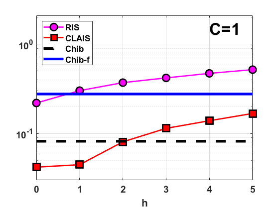
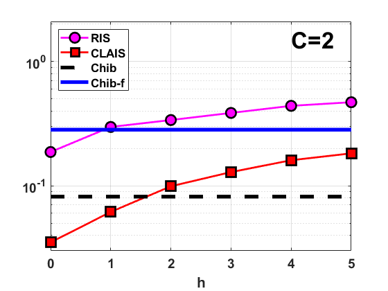
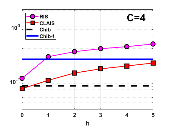
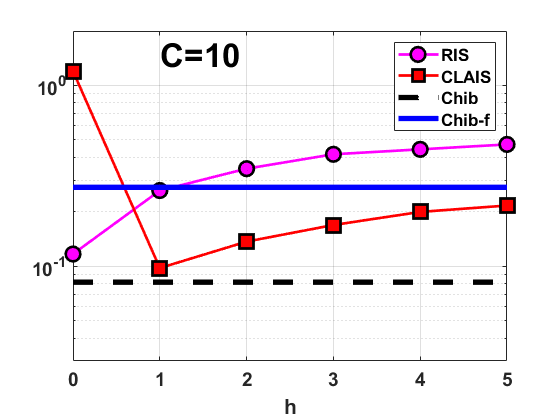
8.5 Experiment with COVID-19 data
Let us consider data representing the number of daily deaths caused by SAR-CoV-2 in Italy from 18 February 2020 to 6 July 2020. Let denote the -th day, we model the each observation as
where is the function that we aim to approximate and ’s are Gaussian perturbations. We consider the approximation of at some as a weighted sum of localized basis functions,
where is -th basis centered at with bandwidth . Let also be an index denoting the type of basis. We consider , then . When , the model becomes a Relevance Vector Machine (RVM), and the interpolation of all data points (maximum overfitting, with zero fitting error) is possible [98].
We consider different types of basis (i.e., ): Gaussian (), Laplacian (), Rectangular () and Triangular-Pyramidal (). Given and , we select the locations as a uniform grid in the interval (recall that ). Hence, knowing and , the locations are given.
Likelihood and prior of . Let be a matrix with elements for and , and let be the vector of coefficients, where is the total number of bases. Then, the observation equation in vector form becomes
where is a vector of noise. We assume normality , where is the identity matrix. Therefore, the likelihood function is . We also consider a Gaussian prior density over the vector of coefficients , i.e., .
where and . Given , , and .
Thus, the complete set of parameters is .
Posteriors and marginalization. With our choice of , the posterior of is also Gaussian,
and a likelihood marginalized w.r.t. is available in closed-form,
| (206) |
For further details see [98]. Now, we consider priors over , and study the following posterior
where , , are folded-Gaussian pdfs defined on with location and scale parameters , and , respectively. Finally, we want to compute the marginal likelihood of this posterior, i.e.,
| (207) |
Furthermore, assuming a uniform probability mass as prior over , we can also marginalize out ,
| (208) |
Considering also a uniform prior over , we can obtain .
For approximating , for , we first apply a Naive Monte Carlo (NMC) method with samples. Secondly, we run an MTM algorithm for obtaining the estimator (see Table 13)
and a Markov chain of vectors for .
This generated chain can be also used for obtaining other estimators (e.g., the HM estimator).
We consider the pairs , , in the MTM scheme. Therefore, employs samples.
Goal. Our purpose is: (a) to make inference regarding the parameters of the model , (b) approximate , (c) study the posterior , and (d) obtain the MAP value, , for . We also study the marginal posterior of each of the four candidate bases.
Results. We run once NMC and MTM for all different models and approximate the posterior for each value of . For illustrative reasons, in Figure 15, we show the posterior probabilities of belonging to the intervals , where is an auxiliary index . Thus, the first value, of the curves in Figure 15, represents the probability of , the second value represents the probability of , and so on until the last value, , which represents the probability of . We can observe that, with both techniques, we obtain that is the most probable interval, with a probability generally closer to , hence . Recall that we have possible intervals (values of ), so when we compare with a uniform distribution , the value is quite high. For , the corresponding probabilities are greater than , reaching with NMC in . In Figure 16, we can observe that, with bases, we are already able to obtain a very good fitting to the data.
Thus, a first conclusion is that the results obtained with models such as RVMs and Gaussian Processes (GPs) (both having [98]) can be approximated in a very good way with a much more scalable model, as our model here with [98]. Regarding the marginal posterior , we can observe the results in Table 20. The basis is discarded since is clearly not appropriate, as also shown graphically by Figure 16. With the results provided by NMC, we prefer slightly the Laplacian basis whereas, with the results of MTM, we have almost . These considerations are reasonable after having a look to Figure 16. As future work, it would be interesting to consider the locations of the bases , for , as additional parameters to be learnt.
| Method | Number of used samples | ||||
|---|---|---|---|---|---|
| NMC | 0.3091 | 0.3307 | 0.0813 | 0.2790 | |
| MTM | 0.3155 | 0.3100 | 0.0884 | 0.2861 |
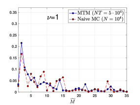
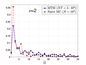
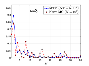
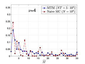
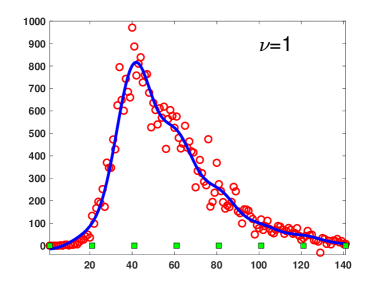
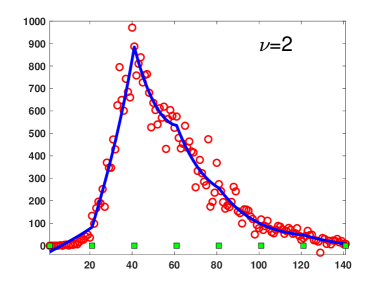
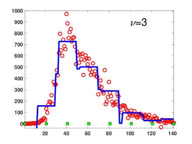
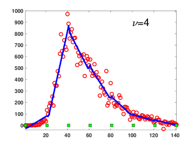
9 Final discussion
In this work, we have provided an exhaustive review of the techniques for marginal likelihood computation with the purpose of model selection and hypothesis testing. Methods for approximating ratios of normalizing constants have been also described. The relationships among all of them have been widely described in the text, for instance in Sections 4.2.2 and 4.3.5, by means of several summary tables (see, as examples, Tables 5, 8, and 16) and Figures from 1 to 6.
The careful choice of the prior and the careful use of the improper priors in the Bayesian setting have been discussed. A brief description of alternative model selection strategies based on the posterior predictive approach, has been also provided.
Most of the presented computational techniques are based on the importance sampling (IS) approach, but also require the use of MCMC algorithms.
Table 21 summarizes some methods for estimating , which involve the generation of the posterior (without using other tempered versions). This table is devoted to the interested readers which desire to obtain samples by an MCMC method with invariant pdf (without either any tempering or sequence of densities) and, at the same time, also desire to approximate . Clearly, this table provides only a subset of all the possible techniques. They can be considered the simplest schemes, in the sense that they do not use any tempering strategy or sequence of densities. We also recall that AIC and DIC are commonly used for model comparison, although they do not directly target the actual marginal likelihood. Table 22 enumerates all the schemes that require the sampling and evaluation of tempered posteriors. For LAIS, the use of tempered posteriors is not strictly required. In PS, one could select a path that does not involve tempered posteriors. The schemes which provides unbiased estimators of or are given in Table 23.
We also provide some final advice for practical use. First of all, if informative priors are not available, a very careful choice of the priors must be considered, as remarked in Sections 7.1 and 7.2, or alternatively a predictive posterior approach should be applied (see Section 7.4). From a computational point of view, our suggestions are listed below:
-
•
The use of Naive Monte Carlo (NMC) should be always considered, at least as a first attempt. Moreover, the HM estimator is surely the worst estimator of , but it could be applied for obtaining an upper bound for , although it can be very imprecise/loose.
-
•
The application of an MTM method is a good choice within the MCMC schemes. In fact, as shown in Figure 17, it also provides two estimators of , as well as a set of samples. These samples can be employed in other estimators, including Chib, RIS and LAIS, for instance.
-
•
Regarding the more general task of estimating ratio of constants, In [48], the authors show that (given two unnormalized pdfs) the optimal umbrella estimator provides the best performance theoretically in estimating the ratio of their normalizing constants. However, the optimal umbrella sampling estimator is difficult and costly to implement (due to the fact sampling from the optimal umbrella proposal is not straightforward), so its best performance may not be achieved in practice.
-
•
The Chib’s method is a good alternative, that provide very good performance as we can observe in Section 8.4 and also in [99, 100]. Moreover, the Chib’s method is also related to bridge sampling as discussed in Section 4.2.2. However, since it requires internal information regarding the MCMC employed (proposal, acceptance function etc.), it cannot be considered for a possible post-processing scheme after obtaining a Markov chain from a black-box MCMC algorithm. This could be easily done with the HM estimator or LAIS, for instance.
-
•
LAIS can be considered a scheme in between the NMC and HM. NMC draw samples from the prior, which makes it rather inefficient in some setting. The HM estimator uses posterior samples but it is very unstable. LAIS uses the posterior samples to build a suitable normalized proposal, so it benefits from localizing samples in regions of high posterior probability (like the HM), while preserving the properties of standard IS (like the Naive MC). In this sense, bridge sampling, the SS method, path sampling, and the rest of techniques based on tempered posteriors, are also schemes in between the NMC and HM.
-
•
The methods based on tempered posteriors provide very good performance but the choice of the temperature parameters is important. In our opinion, among SS, PS, PP, An-IS, and SMC, the more robust to the choice of the ’s is the SS method (that is, perhaps, also the simplest one). Moreover, The SS method does not require the use of several tempered posteriors, unlike PS and PP. The LAIS technique can also be employed in the upper layer. Since the samples in the upper layer are only used as means of other proposal pdfs and, in the lower layer, the true posterior is always evaluated, LAIS is also quite robust to the choice of . More comparisons among SS, An-IS, and SMC are required, since these methods are also very related as depicted in Figures 2, 4, 5 and 6.
-
•
The nested sampling technique has gained attention and is largely applied in the literature. The derivation is complex and several approximations are considered, as discussed in Section 6.2.2. The sampling from the truncated priors is the key point and it is not straightforward [86]. In this sense, its success in the literature is surprising. However, the nested sampling includes an implicit optimization of the likelihood. We believe that is an important feature, since the knowledge of high probabilities of the likelihood is a crucial point also to the rest of computational schemes.
| Method | Section | Need of | Comments |
|---|---|---|---|
| drawing additional samples | |||
| Below: methods for post-processing after generating MCMC samples from . | |||
| Laplace | 3.1 | —– | use MCMC for estimating |
| BIC | 3.2 | —– | use MCMC for estimating |
| KDE | 3.3 | —– | use MCMC for generating samples |
| Bridge | 4.2.1 | additional samples are required; | |
| see Eq. (61) | |||
| RIS | 4 | —– | the HM estimator is a special case |
| MTM | 5.3 | —– | provides two estimators of |
| LAIS | 5.4 | with in the upper-layer | |
| Below: methods that require internal information of the MCMC scheme. | |||
| Chib’s method | 3.4 | additional samples are required | |
| if the proposal is not independent | |||
| MTM | 5.3 | —– | provides two estimators of |
| Below: for model selection but do not approximate the marginal likelihood | |||
| AIC | 3.2 | —– | use MCMC for estimating |
| DIC | 3.2 | —– | use MCMC for estimating and |
| Method | Section | Use of tempering strictly required |
|---|---|---|
| IS-P | 4.3.2 | without tempering, it is HM |
| Stepping Stones (SS) | 4.3.3 | |
| Path Sampling (PS) | 4.3.4 | other paths (without tempering) can be used |
| Method of Power Posteriors (PP) | 4.3.6 | |
| Annealed Importance Sampling (An-IS) | 5.1.2 | |
| Sequential Monte Carlo (SMC) | 5.2 | |
| Layered Adaptive Importance Sampling (LAIS) | 5.4 | — |
| Method | Section |
|---|---|
| Unbiased estimators of : | |
| IS vers-1 | 4 |
| Stepping Stones (SS) | 4.3.3 |
| Annealed Importance Sampling (An-IS) | 5.1.2 |
| Sequential Monte Carlo (SMC) | 5.2 |
| Layered Adaptive Importance Sampling (LAIS) | 5.4 |
| Unbiased estimators of : | |
| Path Sampling (PS) | 4.3.4 |
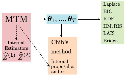
References
- Liu [2004] J. S. Liu, Monte Carlo Strategies in Scientific Computing. Springer, 2004.
- Robert and Casella [2004] C. P. Robert and G. Casella, Monte Carlo Statistical Methods. Springer, 2004.
- Stoltz and Rousset [2010] G. Stoltz and M. Rousset, “Free energy computations: A mathematical perspective,” World Scientific, 2010.
- Liang et al. [2010] F. Liang, C. Liu, and R. Caroll, Advanced Markov Chain Monte Carlo Methods: Learning from Past Samples. England: Wiley Series in Computational Statistics, 2010.
- Balasubramanian [1997] V. Balasubramanian, “Statistical inference, Occam’s razor, and statistical mechanics on the space of probability distributions,” Neural computation, vol. 9, no. 2, pp. 349–368, 1997.
- LaMont and Wiggins [2019] C. H. LaMont and P. A. Wiggins, “Correspondence between thermodynamics and inference,” Physical Review E, vol. 99, no. 5, p. 052140, 2019.
- Sakamoto et al. [1986] Y. Sakamoto, M. Ishiguro, and G. Kitagawa, “Akaike information criterion statistics,” Dordrecht, The Netherlands: D. Reidel, vol. 81, 1986.
- Claeskens and Hjort [2003] G. Claeskens and N. L. Hjort, “The focused information criterion,” Journal of the American Statistical Association, vol. 98, no. 464, pp. 900–916, 2003.
- Spiegelhalter et al. [2002] D. Spiegelhalter, N. G. Best, B. P. Carlin, and A. V. der Linde, “Bayesian measures of model complexity and fit,” J. R. Stat. Soc. B, vol. 64, pp. 583–616, 2002.
- Spiegelhalter et al. [2014] ——, “The deviance information criterion: 12 years on,” J. R. Stat. Soc. B, vol. 76, pp. 485–493, 2014.
- Pooley and Marion [2018] C. M. Pooley and G. Marion, “Bayesian model evidence as a practical alternative to deviance information criterion,” Royal Society Open Science, vol. 5, no. 3, pp. 1–16, 2018.
- Grunwald and Roos [2019] P. Grunwald and T. Roos, “Minimum Description Length Revisited,” arXiv:1908.08484, pp. 1–38, 2019.
- Carlin and Chib [1995] B. P. Carlin and S. Chib, “Bayesian model choice via Markov chain Monte Carlo methods,” Journal of the Royal Statistical Society: Series B (Methodological), vol. 57, no. 3, pp. 473–484, 1995.
- Green [1995] P. J. Green, “Reversible jump Markov chain Monte Carlo computation and Bayesian model determination,” Biometrika, vol. 82, no. 4, pp. 711–732, 1995.
- Hastie and Green [2012] D. I. Hastie and P. J. Green, “Model choice using reversible jump Markov chain Monte Carlo,” Statistica Neerlandica, vol. 66, no. 3, pp. 309–338, 2012.
- Dellaportas et al. [2002] P. Dellaportas, J. J. Forster, and I. Ntzoufras, “On Bayesian model and variable selection using MCMC,” Statistics and Computing, vol. 12, no. 1, pp. 27–36, 2002.
- Godsill [2001] S. J. Godsill, “On the relationship between Markov chain Monte Carlo methods for model uncertainty,” Journal of computational and graphical statistics, vol. 10, no. 2, pp. 230–248, 2001.
- Congdon [2006] P. Congdon, “Bayesian model choice based on Monte Carlo estimates of posterior model probabilities,” Computational statistics & data analysis, vol. 50, no. 2, pp. 346–357, 2006.
- Hoeting et al. [1999] J. A. Hoeting, D. Madigan, A. E. Raftery, and C. T. Volinsky, “Bayesian model averaging: a tutorial,” Statistical Science, vol. 14, no. 4, pp. 382–417, 1999.
- Martino et al. [2017a] L. Martino, J. Read, V. Elvira, and F. Louzada, “Cooperative parallel particle filters for on-line model selection and applications to urban mobility,” Digital Signal Processing, vol. 60, pp. 172–185, 2017.
- Urteaga et al. [2016] I. Urteaga, M. F. Bugallo, and P. M. Djurić, “Sequential Monte Carlo methods under model uncertainty,” in 2016 IEEE Statistical Signal Processing Workshop (SSP), 2016, pp. 1–5.
- Knuth et al. [2015] K. H. Knuth, M. Habeck, N. K. Malakar, A. M. Mubeen, and B. Placek, “Bayesian evidence and model selection,” Digital Signal Processing, vol. 47, pp. 50–67, 2015.
- Schwarz et al. [1978] G. Schwarz et al., “Estimating the dimension of a model,” The annals of statistics, vol. 6, no. 2, pp. 461–464, 1978.
- Hannan and Quinn [1979] E. J. Hannan and B. G. Quinn, “The determination of the order of an autoregression,” Journal of the Royal Statistical Society. Series B (Methodological), vol. 41, no. 2, pp. 190–195, 1979.
- Chib [1995] S. Chib, “Marginal likelihood from the Gibbs output,” Journal of the american statistical association, vol. 90, no. 432, pp. 1313–1321, 1995.
- Polson and Scott [2014] N. G. Polson and J. G. Scott, “Vertical-likelihood Monte Carlo,” arXiv preprint arXiv:1409.3601, 2014.
- Weinberg et al. [2012] M. D. Weinberg et al., “Computing the Bayes factor from a Markov chain Monte Carlo simulation of the posterior distribution,” Bayesian Analysis, vol. 7, no. 3, pp. 737–770, 2012.
- Skilling [2006] J. Skilling, “Nested sampling for general Bayesian computation,” Bayesian analysis, vol. 1, no. 4, pp. 833–859, 2006.
- Lewis and Raftery [1997] S. M. Lewis and A. E. Raftery, “Estimating Bayes factors via posterior simulation with the Laplace—Metropolis estimator,” Journal of the American Statistical Association, vol. 92, no. 438, pp. 648–655, 1997.
- DiCiccio et al. [1997] T. J. DiCiccio, R. E. Kass, A. Raftery, and L. Wasserman, “Computing Bayes factors by combining simulation and asymptotic approximations,” Journal of the American Statistical Association, vol. 92, no. 439, pp. 903–915, 1997.
- Rue et al. [2017] H. Rue, A. Riebler, S. H. Sørbye, J. B. Illian, D. P. Simpson, and F. K. Lindgren, “Bayesian computing with INLA: a review,” Annual Review of Statistics and Its Application, vol. 4, pp. 395–421, 2017.
- Konishi and Kitagawa [2008] S. Konishi and G. Kitagawa, Information criteria and statistical modeling. Springer Science & Business Media, 2008.
- Chib and Jeliazkov [2001] S. Chib and I. Jeliazkov, “Marginal likelihood from the Metropolis–Hastings output,” Journal of the American Statistical Association, vol. 96, no. 453, pp. 270–281, 2001.
- Martino and Elvira [2017] L. Martino and V. Elvira, “Metropolis sampling,” Wiley StatsRef: Statistics Reference Online, pp. 1–18, 2017.
- Martino [2018] L. Martino, “A review of multiple try MCMC algorithms for signal processing,” Digital Signal Processing, vol. 75, pp. 134 – 152, 2018.
- Mira and Nicholls [2003] A. Mira and G. Nicholls, “Bridge estimation of the probability density at a point,” Department of Mathematics, The University of Auckland, New Zealand, Tech. Rep., 2003.
- Rasmussen and Ghahramani [2003] C. E. Rasmussen and Z. Ghahramani, “Bayesian Monte Carlo,” Advances in neural information processing systems, pp. 505–512, 2003.
- Gilks and Wild [1992] W. R. Gilks and P. Wild, “Adaptive Rejection Sampling for Gibbs Sampling,” Applied Statistics, vol. 41, no. 2, pp. 337–348, 1992.
- Gilks et al. [1995a] W. R. Gilks, N. G. Best, and K. K. C. Tan, “Adaptive Rejection Metropolis Sampling within Gibbs Sampling,” Applied Statistics, vol. 44, no. 4, pp. 455–472, 1995.
- Martino et al. [2017b] L. Martino, R. Casarin, F. Leisen, and D. Luengo, “Adaptive independent sticky MCMC algorithms,” EURASIP Journal on Advances in Signal Processing (to paper), 2017.
- Martino et al. [2015] L. Martino, J. Read, and D. Luengo, “Independent doubly adaptive rejection Metropolis sampling within Gibbs sampling,” IEEE Transactions on Signal Processing, vol. 63, no. 12, pp. 3123–3138, June 2015.
- Briol et al. [2019] F.-X. Briol, C. J. Oates, M. Girolami, M. A. Osborne, and D. Sejdinovic, “Probabilistic integration: A role in statistical computation?” Statistical Science, vol. 34, no. 1, pp. 1–22, 2019.
- Chen et al. [2012] M. H. Chen, Q. M. Shao, and J. G. Ibrahim, Monte Carlo methods in Bayesian computation. Springer, 2012.
- Bugallo et al. [2017a] M. F. Bugallo, V. Elvira, L. Martino, D. Luengo, J. Miguez, and P. M. Djuric, “Adaptive importance sampling: the past, the present, and the future,” IEEE Signal Processing Magazine, vol. 34, no. 4, pp. 60–79, 2017.
- Gelfand and Dey [1994] A. E. Gelfand and D. K. Dey, “Bayesian model choice: asymptotics and exact calculations,” Journal of the Royal Statistical Society: Series B (Methodological), vol. 56, no. 3, pp. 501–514, 1994.
- Robert and Wraith [2009] C. P. Robert and D. Wraith, “Computational methods for Bayesian model choice,” AIP conference proceedings, vol. 1193, no. 1, pp. 251–262, 2009.
- Wang et al. [2018] Y.-B. Wang, M.-H. Chen, L. Kuo, and P. O. Lewis, “A new Monte Carlo method for estimating marginal likelihoods,” Bayesian analysis, vol. 13, no. 2, p. 311, 2018.
- Chen et al. [1997] M.-H. Chen, Q.-M. Shao et al., “On Monte Carlo methods for estimating ratios of normalizing constants,” The Annals of Statistics, vol. 25, no. 4, pp. 1563–1594, 1997.
- Torrie and Valleau [1977] G. M. Torrie and J. P. Valleau, “Nonphysical sampling distributions in Monte Carlo free-energy estimation: Umbrella sampling,” Journal of Computational Physics, vol. 23, no. 2, pp. 187–199, 1977.
- Chen [1994] M.-H. Chen, “Importance-weighted marginal Bayesian posterior density estimation,” Journal of the American Statistical Association, vol. 89, no. 427, pp. 818–824, 1994.
- Elvira et al. [2019] V. Elvira, L. Martino, D. Luengo, and M. F. Bugallo, “Generalized Multiple Importance Sampling,” Statistical Science, vol. 34, no. 1, pp. 129–155, 2019.
- Meng and Wong [1996] X.-L. Meng and W. H. Wong, “Simulating ratios of normalizing constants via a simple identity: a theoretical exploration,” Statistica Sinica, pp. 831–860, 1996.
- Geyer [1994] C. J. Geyer, “Estimating normalizing constants and reweighting mixtures,” Technical Report, number 568 - School of Statistics, University of Minnesota, 1994.
- Cameron and Pettitt [2014] E. Cameron and A. Pettitt, “Recursive pathways to marginal likelihood estimation with prior-sensitivity analysis,” Statistical Science, vol. 29, no. 3, pp. 397–419, 2014.
- Newton and Raftery [1994] M. A. Newton and A. E. Raftery, “Approximate Bayesian inference with the weighted likelihood bootstrap,” Journal of the Royal Statistical Society: Series B (Methodological), vol. 56, no. 1, pp. 3–26, 1994.
- Elvira et al. [2016] V. Elvira, L. Martino, D. Luengo, and M. F. Bugallo, “Heretical multiple importance sampling,” IEEE Signal Processing Letters, vol. 23, no. 10, pp. 1474–1478, 2016.
- Elvira et al. [2015] ——, “Efficient multiple importance sampling estimators,” IEEE Signal Processing Letters, vol. 22, no. 10, pp. 1757–1761, 2015.
- Liu et al. [2015] Q. Liu, J. Peng, A. Ihler, and J. Fisher III, “Estimating the partition function by discriminance sampling,” in Proceedings of the Thirty-First Conference on Uncertainty in Artificial Intelligence, 2015, pp. 514–522.
- Gelman and Meng [1998] A. Gelman and X. L. Meng, “Simulating normalizing constants: From importance sampling to bridge sampling to path sampling,” Statistical science, pp. 163–185, 1998.
- Friel and Pettitt [2008] N. Friel and A. N. Pettitt, “Marginal likelihood estimation via power posteriors,” Journal of the Royal Statistical Society: Series B (Statistical Methodology), vol. 70, no. 3, pp. 589–607, 2008.
- Friel et al. [2014] N. Friel, M. Hurn, and J. Wyse, “Improving power posterior estimation of statistical evidence,” Statistics and Computing, vol. 24, no. 5, pp. 709–723, 2014.
- Oates et al. [2016] C. J. Oates, T. Papamarkou, and M. Girolami, “The controlled thermodynamic integral for Bayesian model evidence evaluation,” Journal of the American Statistical Association, vol. 111, no. 514, pp. 634–645, 2016.
- Xie et al. [2010] W. Xie, P. O. Lewis, Y. Fan, L. Kuo, and M. H. Chen, “Improving marginal likelihood estimation for Bayesian phylogenetic model selection,” Systematic biology, vol. 60, no. 2, pp. 150–160, 2010.
- Martino et al. [2018a] L. Martino, V. Elvira, and G. Camps-Valls, “Group importance sampling for particle filtering and MCMC,” Digital Signal Processing, vol. 82, pp. 133 – 151, 2018.
- Chopin [2002] N. Chopin, “A sequential particle filter for static models,” Biometrika, vol. 89, pp. 539–552, 2002.
- Neal [2001] R. M. Neal, “Annealed importance sampling,” Statistics and Computing, vol. 11, no. 2, pp. 125–139, 2001.
- Gilks and Berzuini [2001] W. R. Gilks and C. Berzuini, “Following a moving target-Monte Carlo inference for dynamic Bayesian models,” Journal of the Royal Statistical Society. Series B (Statistical Methodology), vol. 63, no. 1, pp. 127–146, 2001.
- Moral et al. [2006] P. D. Moral, A. Doucet, and A. Jasra, “Sequential Monte Carlo samplers,” Journal of the Royal Statistical Society: Series B (Statistical Methodology), vol. 68, no. 3, pp. 411–436, 2006.
- Martino et al. [2017c] L. Martino, V. Elvira, and M. F. Louzada, “Effective Sample Size for importance sampling based on the discrepancy measures,” Signal Processing, vol. 131, pp. 386–401, 2017.
- Martino et al. [2016] L. Martino, V. Elvira, and F. Louzada, “Weighting a resampled particle in Sequential Monte Carlo,” IEEE Statistical Signal Processing Workshop, (SSP), vol. 122, pp. 1–5, 2016.
- Naesseth et al. [2015] C. A. Naesseth, F. Lindsten, and T. B. Schon, “Nested Sequential Monte Carlo methods,” Proceedings of theInternational Conference on Machine Learning, vol. 37, pp. 1–10, 2015.
- Cappé et al. [2004] O. Cappé, A. Guillin, J. M. Marin, and C. P. Robert, “Population Monte Carlo,” Journal of Computational and Graphical Statistics, vol. 13, no. 4, pp. 907–929, 2004.
- Kong [1992] A. Kong, “A note on importance sampling using standardized weights,” Technical Report 348, Department of Statistics, University of Chicago, 1992.
- Djurić et al. [2003] P. M. Djurić, J. H. Kotecha, J. Zhang, Y. Huang, T. Ghirmai, M. F. Bugallo, and J. Míguez, “Particle filtering,” IEEE Signal Processing Magazine, vol. 20, no. 5, pp. 19–38, September 2003.
- Doucet and Johansen [2008] A. Doucet and A. M. Johansen, “A tutorial on particle filtering and smoothing: fifteen years later,” technical report, 2008.
- Martino and Read [2013] L. Martino and J. Read, “On the flexibility of the design of multiple try Metropolis schemes,” Computational Statistics, vol. 28, no. 6, pp. 2797–2823, 2013.
- Martino et al. [2012] L. Martino, V. P. D. Olmo, and J. Read, “A multi-point Metropolis scheme with generic weight functions,” Statistics & Probability Letters, vol. 82, no. 7, pp. 1445–1453, 2012.
- Bugallo et al. [2017b] M. F. Bugallo, V. Elvira, L. Martino, D. Luengo, J. Miguez, and P. M. Djuric, “Adaptive importance sampling: The past, the present, and the future,” IEEE Signal Processing Magazine, vol. 34, no. 4, pp. 60–79, 2017.
- Bugallo et al. [2015] M. F. Bugallo, L. Martino, and J. Corander, “Adaptive importance sampling in signal processing,” Digital Signal Processing, vol. 47, pp. 36–49, 2015.
- Martino et al. [2017d] L. Martino, V. Elvira, D. Luengo, and J. Corander, “Layered adaptive importance sampling,” Statistics and Computing, vol. 27, no. 3, pp. 599–623, 2017.
- Schuster and Klebanov [2018] I. Schuster and I. Klebanov, “Markov Chain Importance Sampling-a highly efficient estimator for MCMC,” arXiv preprint arXiv:1805.07179, 2018.
- Cornuet et al. [2012] J. M. Cornuet, J. M. Marin, A. Mira, and C. P. Robert, “Adaptive multiple importance sampling,” Scandinavian Journal of Statistics, vol. 39, no. 4, pp. 798–812, December 2012.
- Martino and Elvira [2018] L. Martino and V. Elvira, “Compressed Monte Carlo for distributed Bayesian inference,” viXra:1811.0505, 2018.
- Martino et al. [2017e] L. Martino, V. Elvira, and D. Luengo, “Anti-tempered layered adaptive importance sampling,” International Conference on Digital Signal Processing (DSP), 2017.
- Martino et al. [2018b] L. Martino, D. Luengo, and J. Míguez, “Independent random sampling methods,” Springer, 2018.
- Chopin and Robert [2010] N. Chopin and C. P. Robert, “Properties of nested sampling,” Biometrika, vol. 97, no. 3, pp. 741–755, 2010.
- Kass and Raftery [1995] R. E. Kass and A. E. Raftery, “Bayes factors,” Journal of the american statistical association, vol. 90, no. 430, pp. 773–795, 1995.
- Spiegelhalter and Smith [1982] D. J. Spiegelhalter and A. F. Smith, “Bayes factors for linear and log-linear models with vague prior information,” Journal of the Royal Statistical Society: Series B (Methodological), vol. 44, no. 3, pp. 377–387, 1982.
- O’Hagan [1995] A. O’Hagan, “Fractional Bayes factors for model comparison,” Journal of the Royal Statistical Society: Series B (Methodological), vol. 57, no. 1, pp. 99–118, 1995.
- Berger and Pericchi [1996] J. O. Berger and L. R. Pericchi, “The intrinsic Bayes factor for model selection and prediction,” Journal of the American Statistical Association, vol. 91, no. 433, pp. 109–122, 1996.
- Luengo et al. [2020] D. Luengo, L. Martino, M. Bugallo, V. Elvira, and S. S., “A survey of monte carlo methods for parameter estimation,” EURASIP J. Adv. Signal Process., vol. 25, pp. 1–62, 2020.
- Gelman et al. [2013] A. Gelman, J. B. Carlin, H. S. Stern, D. B. Dunson, A. Vehtari, and D. B. Rubin, Bayesian data analysis. CRC press, 2013.
- Piironen and Vehtari [2017] J. Piironen and A. Vehtari, “Comparison of Bayesian predictive methods for model selection,” Statistics and Computing, vol. 27, no. 3, pp. 711–735, 2017.
- Vehtari et al. [2017] A. Vehtari, A. Gelman, and J. Gabry, “Practical Bayesian model evaluation using leave-one-out cross-validation and WAIC,” Statistics and computing, vol. 27, no. 5, pp. 1413–1432, 2017.
- Fong and Holmes [2020] E. Fong and C. Holmes, “On the marginal likelihood and cross-validation,” Biometrika, vol. 107, no. 2, pp. 489–496, 2020.
- Alston et al. [2005] C. Alston, P. Kuhnert, L. S. Choy, R. McVinish, and K. Mengersen, “Bayesian model comparison: Review and discussion,” International Statistical Insitute, 55th session, 2005.
- O’Hara and Sillanpää [2009] R. B. O’Hara and M. J. Sillanpää, “A review of Bayesian variable selection methods: what, how and which,” Bayesian analysis, vol. 4, no. 1, pp. 85–117, 2009.
- Martino and Read [2020] L. Martino and J. Read, “Joint introduction to Gaussian Processes and Relevance Vector Machines with connections to Kalman filtering and other kernel smoothers,” arXiv:2009.09217, pp. 1–50, 2020.
- Marin and Robert [2009] J. M. Marin and C. P. Robert, “Importance sampling methods for Bayesian discrimination between embedded models,” arXiv preprint arXiv:0910.2325, 2009.
- Friel and Wyse [2012] N. Friel and J. Wyse, “Estimating the evidence-a review,” Statistica Neerlandica, vol. 66, no. 3, pp. 288–308, 2012.
- Gilks et al. [1995b] W. R. Gilks, S. Richardson, and D. Spiegelhalter, Markov chain Monte Carlo in practice. Chapman and Hall/CRC, 1995.
- Bos [2002] C. S. Bos, “A comparison of marginal likelihood computation methods,” in Compstat. Springer, 2002, pp. 111–116.
- Vyshemirsky and Girolami [2007] V. Vyshemirsky and M. A. Girolami, “Bayesian ranking of biochemical system models,” Bioinformatics, vol. 24, no. 6, pp. 833–839, 2007.
- Ardia et al. [2012] D. Ardia, N. Baştürk, L. Hoogerheide, and H. K. Van Dijk, “A comparative study of Monte Carlo methods for efficient evaluation of marginal likelihood,” Computational Statistics & Data Analysis, vol. 56, no. 11, pp. 3398–3414, 2012.
- Schöniger et al. [2014] A. Schöniger, T. Wöhling, L. Samaniego, and W. Nowak, “Model selection on solid ground: Rigorous comparison of nine ways to evaluate Bayesian model evidence,” Water resources research, vol. 50, no. 12, pp. 9484–9513, 2014.
- Liu et al. [2016] P. Liu, A. S. Elshall, M. Ye, P. Beerli, X. Zeng, D. Lu, and Y. Tao, “Evaluating marginal likelihood with thermodynamic integration method and comparison with several other numerical methods,” Water Resources Research, vol. 52, no. 2, pp. 734–758, 2016.
- Zhao and Severini [2017] Z. Zhao and T. A. Severini, “Integrated likelihood computation methods,” Computational Statistics, vol. 32, no. 1, pp. 281–313, 2017.
- R Oaks et al. [2019] J. R Oaks, K. A. Cobb, V. N Minin, and A. D. Leaché, “Marginal likelihoods in phylogenetics: a review of methods and applications,” Systematic biology, vol. 68, no. 5, pp. 681–697, 2019.
Appendix A Table of other reviews
The related literature is rather vast. In this section, we provide a brief summary that intends to be illustrative rather than exhaustive, by means of Table 24. The most relevant (in our opinion) and related surveys are compared according to the topics, material and schemes described in lthe work. The proportion of covering and overlapping with this work is roughly classified as “partial” , “complete” , “remarkable” or “more exhaustive” work with . From Table 24, we can also notice the completeness of this work. We take into account also the completeness and the depth of details provided in the different derivations. The Christian Robert’s blog deserves a special mention (https://xianblog.wordpress.com), since Professor C. Robert has devoted several entries of his blog with very interesting comments regarding the marginal likelihood estimation and related topics.
| Surveys | Families 1–2 | IS | Advanced schemes | Vertical likelihood | Improper | |||||||||
| 1 prop. | 2 prop. | Multiple | MCMC within IS | MTM | AIS | 5.1 | 5.2 | 5.3 | ||||||
| Gelfand and Dey (1994)[45] | ||||||||||||||
| Kass and Raftery (1995)[87] | ||||||||||||||
| Raftery (1995)[101, Ch. 10] | ||||||||||||||
| Meng and Wong (1996)[52] | ||||||||||||||
| DiCiccio et al (1997)[30] | ||||||||||||||
| Chen and Shao (1997)[48] | ||||||||||||||
| Chen et al (2012)[43, Ch. 5] | ||||||||||||||
| Gelman and Meng (1997)[59] | ||||||||||||||
| Bos (2002)[102] | ||||||||||||||
| Vyshemirsky and Girolami (2007)[103] | ||||||||||||||
| Marin and Robert (2009)[99] | ||||||||||||||
| Robert and Wraith (2009)[46] | ||||||||||||||
| Friel and Wyse (2012)[100] | ||||||||||||||
| Ardia et al (2012)[104] | ||||||||||||||
| Polson and Scott (2014)[26] | ||||||||||||||
| Sch niger et al (2014)[105] | ||||||||||||||
| Knuth et al (2015)[22] | ||||||||||||||
| Liu et al (2016)[106] | ||||||||||||||
| Zhao and Severini (2017)[107] | ||||||||||||||
| Martino (2018)[35] | ||||||||||||||
| Bugallo et al (2017)[78] | ||||||||||||||
| Bugallo et al (2015)[79] | ||||||||||||||
| Oaks et al (2019)[108] | ||||||||||||||
| O’Hagan (1995)[89] | ||||||||||||||
| Berger and Pericchi (1996)[90] | ||||||||||||||