Inflation from f(R)𝑓𝑅f(R) theories in gravity’s rainbow

Areef Waeming1,†, Phongpichit Channuie1,2,3,4,‡

1School of Science, Walailak University, Nakhon Si Thammarat, 80160, Thailand
2College of Graduate Studies, Walailak University, Nakhon Si Thammarat, 80160, Thailand
3Research Group in Applied, Computational and Theoretical Science (ACTS),
Walailak University, Nakhon Si Thammarat, 80160, Thailand
4Thailand Center of Excellence in Physics, Ministry of Higher Education, Science,
Research and Innovation, Bangkok 10400, Thailand
Email:reef.waeming@gmail.com, channuie@gmail.com


Abstract: In this work, we study the f(R)𝑓𝑅f(R) models of inflation in the context of gravity’s rainbow theory. We choose three types of f(R)𝑓𝑅f(R) models: f(R)=R+α(R/M)n,f(R)=R+αR2+βR2log(R/M2)formulae-sequence𝑓𝑅𝑅𝛼superscript𝑅𝑀𝑛𝑓𝑅𝑅𝛼superscript𝑅2𝛽superscript𝑅2𝑅superscript𝑀2f(R)=R+\alpha(R/M)^{n},\,f(R)=R+\alpha R^{2}+\beta R^{2}\log(R/M^{2}) and the Einstein-Hu-Sawicki model with n,α,β𝑛𝛼𝛽n,\,\alpha,\,\beta being arbitrary real constants. Here R𝑅R and M𝑀M are the Ricci scalar and mass scale, respectively. For all models, the rainbow function is written in the power-law form of the Hubble parameter. We present a detailed derivation of the spectral index of curvature perturbation and the tensor-to-scalar ratio and compare the predictions of our results with latest Planck 2018 data. With the sizeable number of e-foldings and proper choices of parameters, we discover that the predictions of all f(R)𝑓𝑅f(R) models present in this work are in excellent agreement with the Planck analysis.


1 Introduction

As an effective theory of gravity, Einstein’s general theory of gravity is valid in the low energy regime (IR), while at very high energy regime (UV) the Einstein theory could in principle be improved. It is expected that the usual dispersion relation will get modified at the energy scale of the order of Planck length in various theories of quantum gravity. Deformations of dispersion relations are timely since the Cherenkov array [1] will focus on this type of deformations as well. In Ref.[2], Magueijo and Smolin introduced a modification of the dispersion relation by replacing the standard one, i.e. ϵ2p2=m2superscriptitalic-ϵ2superscript𝑝2superscript𝑚2\epsilon^{2}-p^{2}=m^{2}, replaced with a new form ϵ2f~2(ϵ)p2g~2(ϵ)=m2superscriptitalic-ϵ2superscript~𝑓2italic-ϵsuperscript𝑝2superscript~𝑔2italic-ϵsuperscript𝑚2\epsilon^{2}{\tilde{f}}^{2}(\epsilon)-p^{2}{\tilde{g}}^{2}(\epsilon)=m^{2} where f~(ϵ)~𝑓italic-ϵ{\tilde{f}}(\epsilon) and g~(ϵ)~𝑔italic-ϵ{\tilde{g}}(\epsilon) are so-called rainbow functions. They are required to satisfy standard properties at a low-energy IR limit when ϵ/M0italic-ϵ𝑀0\epsilon/M\rightarrow 0 that f~(ϵ/M)1~𝑓italic-ϵ𝑀1{\tilde{f}}(\epsilon/M)\rightarrow 1 and g~(ϵ/M)1~𝑔italic-ϵ𝑀1{\tilde{g}}(\epsilon/M)\rightarrow 1 where M𝑀M is the energy scale that quantum effects of gravity become relevant.

It is expected that the usual dispersion relation in the UV limit has to be in principle reformed and captures a modification of the geometry at that limit. One way to think about this is to assume that the geometry of the space-time in gravity’s rainbow depends on energy of the test particles. Therefore, each test particle carrying different energy will feel a different geometry of space-time. This behavior promotes a family of metrics, namely a rainbow metric, characterized by ϵitalic-ϵ\epsilon to describe the background of the space-time instead of a single metric. In gravity’s rainbow, the modified metric can be expressed as

g(ϵ)=ημνe~μ(ϵ)e~ν(ϵ),𝑔italic-ϵtensor-productsuperscript𝜂𝜇𝜈subscript~𝑒𝜇italic-ϵsubscript~𝑒𝜈italic-ϵ\displaystyle g(\epsilon)=\eta^{\mu\nu}{\tilde{e}}_{\mu}(\epsilon)\otimes{\tilde{e}}_{\nu}(\epsilon)\,, (1.1)

where the energy dependence of the frame field e~μ(ϵ)subscript~𝑒𝜇italic-ϵ{\tilde{e}}_{\mu}(\epsilon) can be written in terms of the energy independence frame field eμsubscript𝑒𝜇e_{\mu} as e~0(ϵ)=e0/f~(ϵ)subscript~𝑒0italic-ϵsubscript𝑒0~𝑓italic-ϵ{\tilde{e}}_{0}(\epsilon)=e_{0}/{\tilde{f}}(\epsilon) and e~i(ϵ)=ei/g~(ϵ)subscript~𝑒𝑖italic-ϵsubscript𝑒𝑖~𝑔italic-ϵ{\tilde{e}}_{i}(\epsilon)=e_{i}/{\tilde{g}}(\epsilon) where i=1,2,3𝑖123i=1,2,3. In the cosmological viewpoint, the conventional FLRW spacetime metric for homogeneous and isotropic universe is replaced by a rainbow metric of the form

ds2(ϵ)=dt2f~2(ϵ)+a2(t)g~2(ϵ)δijdxidxj,𝑑superscript𝑠2italic-ϵ𝑑superscript𝑡2superscript~𝑓2italic-ϵsuperscript𝑎2𝑡superscript~𝑔2italic-ϵsubscript𝛿𝑖𝑗𝑑superscript𝑥𝑖𝑑superscript𝑥𝑗\displaystyle{ds}^{2}(\epsilon)=-\frac{dt^{2}}{\tilde{f}^{2}(\epsilon)}+\frac{a^{2}(t)}{\tilde{g}^{2}(\epsilon)}\delta_{ij}{dx}^{i}{dx}^{j}\,, (1.2)

where a(t)𝑎𝑡a(t) is a scale factor. In Ref.[3], the author studied the semi-classical effect of radiation particles on the background metric in the framework of rainbow gravity, and obtained the modified FLRW equations where the energy of particles varies with the cosmological time. In the present work, for very early universe, we consider the rainbow functions f~(ϵ)~𝑓italic-ϵ{\tilde{f}}(\epsilon) dependent on time implicitly through the energy of particles.

In recent years, a framework of gravity’s rainbow has attracted a lot of attentions and became the subject of much interest in the literature. Among many relevant publications, various physical properties of the black holes have been investigated, see e.g. [20, 21, 4, 5, 6, 7, 8, 9, 10, 11, 12, 13, 14, 15, 16, 17, 18, 19]. Moreover, the effects of the rainbow functions have also been discussed in other cosmological scenarios, see for instance [22, 23, 24, 25, 26, 27, 28, 29]. It was found that the gravity’s rainbow was investigated in Gauss-Bonnet gravity [30], massive gravity [31, 32] and f(R)𝑓𝑅f(R) gravity [33]. More specifically, the gravity’s rainbow has also been used for analyzing the effects of rainbow functions on the Starobinsky model of f(R)𝑓𝑅f(R) gravity [34]. More recently, the deformed Starobinsky model [35] has been also studied in the context of gravity’s rainbow [36].

This paper is organized as follows: In section 2, we formulate f(R)𝑓𝑅f(R) theory [39, 40] in the framework of gravity’s rainbow. We study the f(R)𝑓𝑅f(R) models of inflation in the context of gravity’s rainbow theory by considering three types of f(R)𝑓𝑅f(R) models: f(R)=R+α(R/M)n,f(R)=R+αR2+βR2log(R/M2)formulae-sequence𝑓𝑅𝑅𝛼superscript𝑅𝑀𝑛𝑓𝑅𝑅𝛼superscript𝑅2𝛽superscript𝑅2𝑅superscript𝑀2f(R)=R+\alpha(R/M)^{n},\,f(R)=R+\alpha R^{2}+\beta R^{2}\log(R/M^{2}) and the Einstein-Hu-Sawicki model. We take a short review of a cosmological linear perturbation in the context of the gravity’s rainbow generated during inflation. Here we compute the spectral index of scalar perturbation and the tensor-to-scalar ratio of the model in section 3. In section 4, we compare the predicted results with Planck 2018 data. We conclude our findings in the last section. In this work, we use the metric signature (,+,+,+)(-,+,+,+). The Greek indices μ,ν,ρ,𝜇𝜈𝜌\mu,\nu,\rho,... run from 00 to 333, whereas the Latin indices i,j,k,𝑖𝑗𝑘i,j,k,... run from 111 to 333 (spatial components).

2 General Setup: f(R)𝑓𝑅f(R) gravity’s rainbow

As is well known, Einstein’s theory of gravitation remains a pillar of modern description of gravity as a fundamental property of space-time. However, the theory itself is plagued by major unsolved problems nowadays, e.g. dark matter, dark energy and even cosmic inflation. Hence, the modification to general relativity are expected to be plausible in the very early universe where possible corrections to Einstein’s theory may in principle appear at high curvature. One of the simplest classes of such modifications is to replace the Einstein-Hilbert term in the action with a generic function of the Ricci scalar. This class of theories is known as the f(R)𝑓𝑅f(R) theories. Note that there were much earlier and pioneer works on f(R)𝑓𝑅f(R) and other gravity theories, see [37, 38]. Here we initiate our setup with the traditionally 4-dimensional action in f(R)𝑓𝑅f(R) gravity including the matter fields as [39, 40].

S=12κ2d4xgf(R)+d4xgM(gμν,ΨM),𝑆12superscript𝜅2superscript𝑑4𝑥𝑔𝑓𝑅superscript𝑑4𝑥𝑔subscript𝑀subscript𝑔𝜇𝜈subscriptΨ𝑀\displaystyle S=\frac{1}{2\kappa^{2}}\int d^{4}x\sqrt{-g}f(R)+\int d^{4}x\sqrt{-g}{\cal L}_{M}(g_{\mu\nu},\Psi_{M})\,, (2.1)

where we have defined κ2=8πG=8π/mP2superscript𝜅28𝜋𝐺8𝜋subscriptsuperscript𝑚2P\kappa^{2}=8\pi G=8\pi/m^{2}_{\rm P}, g𝑔g is the determinant of the metric gμνsubscript𝑔𝜇𝜈g_{\mu\nu}, and the matter field Lagrangian Msubscript𝑀{\cal L}_{M} depends on gμνsubscript𝑔𝜇𝜈g_{\mu\nu} and matter fields ΨMsubscriptΨ𝑀\Psi_{M}. The field equation can be directly derived by performing variation of the action (2.1) with respect to gμνsubscript𝑔𝜇𝜈g_{\mu\nu} to obtain [39, 40]

F(R)Rμν(g)12f(R)gμνμνF(R)+gμνF(R)=κ2Tμν(M),𝐹𝑅subscript𝑅𝜇𝜈𝑔12𝑓𝑅subscript𝑔𝜇𝜈subscript𝜇subscript𝜈𝐹𝑅subscript𝑔𝜇𝜈𝐹𝑅superscript𝜅2subscriptsuperscript𝑇𝑀𝜇𝜈\displaystyle F(R)R_{\mu\nu}(g)-\frac{1}{2}f(R)g_{\mu\nu}-\nabla_{\mu}\nabla_{\nu}F(R)+g_{\mu\nu}\Box F(R)=\kappa^{2}T^{(M)}_{\mu\nu}\,, (2.2)

where F(R)=f(R)/R𝐹𝑅𝑓𝑅𝑅F(R)=\partial f(R)/\partial R and the operator \Box is defined by (1/g)μ(ggμνν)1𝑔subscript𝜇𝑔superscript𝑔𝜇𝜈subscript𝜈\Box\equiv(1/\sqrt{-g})\partial_{\mu}(\sqrt{-g}g^{\mu\nu}\partial_{\nu}). Basically, the energy-momentum tensor of the matter fields is given by a definition Tμν(M)=(2/g)δ(gM)/δgμνsubscriptsuperscript𝑇𝑀𝜇𝜈2𝑔𝛿𝑔subscript𝑀𝛿superscript𝑔𝜇𝜈T^{(M)}_{\mu\nu}=(-2/\sqrt{-g})\delta(\sqrt{-g}{\cal L}_{M})/\delta g^{\mu\nu}. Here it satisfies the continuity equation such that μTμν(M)=0superscript𝜇subscriptsuperscript𝑇𝑀𝜇𝜈0\nabla^{\mu}T^{(M)}_{\mu\nu}=0. As a part the standard approach, it is worth noting that the energy-momentum tensor of matter is given in the perfect fluid form as Tμν(M)=diag(ρ,P,P,P)subscriptsuperscript𝑇𝑀𝜇𝜈diag𝜌𝑃𝑃𝑃T^{(M)}_{\mu\nu}={\rm diag}(-\rho,\,P,\,P,\,P) with ρ𝜌\rho and P𝑃P being the energy density and the pressure, respectively. Now we are going to derive cosmological solutions to field equations (2.2). Inserting the modified FLRW metric (1.2) in the field equations (2.2) and assuming that the stress-energy tensor is written in terms of the perfect fluid form yield

3(FH2+HF˙)6FHg~˙g~+3Fg~˙2g~2+F˙f~˙f~3F˙g~˙g~=FRf(R)2f~2+κ2ρf~2,3𝐹superscript𝐻2𝐻˙𝐹6𝐹𝐻˙~𝑔~𝑔3𝐹superscript˙~𝑔2superscript~𝑔2˙𝐹˙~𝑓~𝑓3˙𝐹˙~𝑔~𝑔𝐹𝑅𝑓𝑅2superscript~𝑓2superscript𝜅2𝜌superscript~𝑓2\displaystyle 3\left(FH^{2}+H\dot{F}\right)-6FH\frac{\dot{\tilde{g}}}{\tilde{g}}+3F\frac{\dot{\tilde{g}}^{2}}{\tilde{g}^{2}}+\dot{F}\frac{\dot{\tilde{f}}}{\tilde{f}}-3\dot{F}\frac{\dot{\tilde{g}}}{\tilde{g}}=\frac{FR-f(R)}{2\tilde{f}^{2}}+\frac{\kappa^{2}\rho}{\tilde{f}^{2}}\,, (2.3)

and

3FH23F˙H+3FH˙+3FHf~˙f~F˙f~˙f~4Fg~˙2g~4+6FHg~˙g~33F˙g~˙g~3+Fg~¨g~3+Ff~˙f~g~˙g~33FH21g~23𝐹superscript𝐻23˙𝐹𝐻3𝐹˙𝐻3𝐹𝐻˙~𝑓~𝑓˙𝐹˙~𝑓~𝑓4𝐹superscript˙~𝑔2superscript~𝑔46𝐹𝐻˙~𝑔superscript~𝑔33˙𝐹˙~𝑔superscript~𝑔3𝐹¨~𝑔superscript~𝑔3𝐹˙~𝑓~𝑓˙~𝑔superscript~𝑔33𝐹superscript𝐻21superscript~𝑔2\displaystyle 3FH^{2}-3\dot{F}H+3F\dot{H}+3FH\frac{\dot{\tilde{f}}}{\tilde{f}}-\dot{F}\frac{\dot{\tilde{f}}}{\tilde{f}}-4F\frac{\dot{\tilde{g}}^{2}}{\tilde{g}^{4}}+6FH\frac{\dot{\tilde{g}}}{\tilde{g}^{3}}-3\dot{F}\frac{\dot{\tilde{g}}}{\tilde{g}^{3}}+F\frac{\ddot{\tilde{g}}}{\tilde{g}^{3}}+F\frac{\dot{\tilde{f}}}{\tilde{f}}\frac{\dot{\tilde{g}}}{\tilde{g}^{3}}-3FH^{2}\frac{1}{\tilde{g}^{2}}
+2F˙H1g~2+F¨g~2FH˙1g~2+6Fg~˙2g~2FHf~˙f~1g~2+F˙f~˙f~1g~26FHg~˙g~+3F˙g~˙g~3Fg~¨g~3Ff~˙f~g~˙g~2˙𝐹𝐻1superscript~𝑔2¨𝐹superscript~𝑔2𝐹˙𝐻1superscript~𝑔26𝐹superscript˙~𝑔2superscript~𝑔2𝐹𝐻˙~𝑓~𝑓1superscript~𝑔2˙𝐹˙~𝑓~𝑓1superscript~𝑔26𝐹𝐻˙~𝑔~𝑔3˙𝐹˙~𝑔~𝑔3𝐹¨~𝑔~𝑔3𝐹˙~𝑓~𝑓˙~𝑔~𝑔\displaystyle+2\dot{F}H\frac{1}{\tilde{g}^{2}}+\frac{\ddot{F}}{\tilde{g}^{2}}-F\dot{H}\frac{1}{\tilde{g}^{2}}+6F\frac{\dot{\tilde{g}}^{2}}{\tilde{g}^{2}}-FH\frac{\dot{\tilde{f}}}{\tilde{f}}\frac{1}{\tilde{g}^{2}}+\dot{F}\frac{\dot{\tilde{f}}}{\tilde{f}}\frac{1}{\tilde{g}^{2}}-6FH\frac{\dot{\tilde{g}}}{\tilde{g}}+3\dot{F}\frac{\dot{\tilde{g}}}{\tilde{g}}-3F\frac{\ddot{\tilde{g}}}{\tilde{g}}-3F\frac{\dot{\tilde{f}}}{\tilde{f}}\frac{\dot{\tilde{g}}}{\tilde{g}}
f(R)(g~1)(g~+1)2f~2g~2=κ2(ρg~2+P)f~2g~2,𝑓𝑅~𝑔1~𝑔12superscript~𝑓2superscript~𝑔2superscript𝜅2𝜌superscript~𝑔2𝑃superscript~𝑓2superscript~𝑔2\displaystyle-\frac{f(R)\left(\tilde{g}-1\right)\left(\tilde{g}+1\right)}{2\tilde{f}^{2}\tilde{g}^{2}}=-\frac{\kappa^{2}\left(\rho\tilde{g}^{2}+P\right)}{\tilde{f}^{2}\tilde{g}^{2}}\,, (2.4)

where we have defined a first and second derivative with respect to time with a˙˙𝑎{\dot{a}} and a¨¨𝑎{\ddot{a}}, respectively. For simplicity, in our analysis below we chose g~=1~𝑔1\tilde{g}=1 and only considered the spatially flat universe. Detailed calculations of the Ricci scalar are given in Appendix A.

2.1 Model I: f(R)=R+α(R/M)n𝑓𝑅𝑅𝛼superscript𝑅𝑀𝑛f(R)=R+\alpha(R/M)^{n}

Modification of the Einstein–Hilbert (EH) action through the Ricci scalar can describe early universe, e.g. cosic inflation. In this first model, we start by considering a simple case of the f(R)𝑓𝑅f(R) gravity model where the Ricci scalar replaced by a new function as

f(R)=R+α(RM)n,𝑓𝑅𝑅𝛼superscript𝑅𝑀𝑛\displaystyle f(R)=R+\alpha\Big{(}\frac{R}{M}\Big{)}^{n}, (2.5)

where α>0𝛼0\alpha>0 and n𝑛n are arbitrary constants assuming that n2𝑛2n\geq 2. Notice that when setting α=1/6𝛼16\alpha=1/6 and n=2𝑛2n=2 we obtain f(R)𝑓𝑅f(R) gravity of Starobinsky model [54]. From Eq.(2.3), we find for this model

3H2+α6n1f~3((2H2+H˙)f~+Hf~˙)2(f~((2H2+H˙)f~+Hf~˙)M)n(H(n1)nf~˙3\displaystyle 3H^{2}+\frac{\alpha 6^{n-1}}{\tilde{f}^{3}\big{(}\big{(}2H^{2}+\dot{H}\big{)}\tilde{f}+H\dot{\tilde{f}}\big{)}^{2}}\Big{(}\frac{\tilde{f}\big{(}\big{(}2H^{2}+\dot{H}\big{)}\tilde{f}+H\dot{\tilde{f}}\big{)}}{M}\Big{)}^{n}\Big{(}H(n-1)n\dot{\tilde{f}}^{3}
+(n1)f~˙f~(f~˙(H2(7n3)+3H˙n)+Hnf~¨)+((n1)nf~˙H¨+H((3H2(n(4n7)+4)\displaystyle+(n-1)\dot{\tilde{f}}\tilde{f}\big{(}\dot{\tilde{f}}\big{(}H^{2}(7n-3)+3\dot{H}n\big{)}+Hn\ddot{\tilde{f}}\big{)}+\big{(}(n-1)n\dot{\tilde{f}}\ddot{H}+H\big{(}\big{(}3H^{2}(n(4n-7)+4)
+H˙(n1)(13n6))f~˙+3H(n1)nf~¨))f~2+3(2H4(n2)+H2H˙(n(4n7)+4)\displaystyle+\dot{H}(n-1)(13n-6)\big{)}\dot{\tilde{f}}+3H(n-1)n\ddot{\tilde{f}}\big{)}\big{)}\tilde{f}^{2}+3\big{(}-2H^{4}(n-2)+H^{2}\dot{H}(n(4n-7)+4)
+H(n1)nH¨+H˙2((n1)))f~3)=0,\displaystyle+H(n-1)n\ddot{H}+\dot{H}^{2}(-(n-1))\big{)}\tilde{f}^{3}\Big{)}=0, (2.6)

and

13R3f~2(α(n1)nRf~(RM)n(R˙(9Hf~+4f~˙)+3f~R¨)+3α(n2)(n1)nR˙2f~2(RM)n\displaystyle\frac{1}{3R^{3}\tilde{f}^{2}}\Bigg{(}\alpha(n-1)nR\tilde{f}\Big{(}\frac{R}{M}\Big{)}^{n}\big{(}\dot{R}\big{(}9H\tilde{f}+4\dot{\tilde{f}}\big{)}+3\tilde{f}\ddot{R}\big{)}+3\alpha(n-2)(n-1)n\dot{R}^{2}\tilde{f}^{2}\Big{(}\frac{R}{M}\Big{)}^{n}
α(n2)R3(RM)n+R4)=0.\displaystyle-\alpha(n-2)R^{3}\Big{(}\frac{R}{M}\Big{)}^{n}+R^{4}\Bigg{)}=0. (2.7)

Here we are only interested in an inflationary solution. Therefore we invoke the slow-roll approximations. Hence the terms containing H¨¨𝐻\ddot{H} and higher power in H˙˙𝐻\dot{H} can be neglected in this particular regime. It is rather straightforward to show that the Eq.(2.6) is reduced to

H˙˙𝐻\displaystyle\dot{H} H2212n3nα(λ+1)(4n27n+4)(H2(HM)2λM)nsimilar-to-or-equalsabsentsuperscript𝐻2superscript212𝑛superscript3𝑛𝛼𝜆14superscript𝑛27𝑛4superscriptsuperscript𝐻2superscript𝐻𝑀2𝜆𝑀𝑛\displaystyle\simeq\frac{H^{2}2^{1-2n}3^{-n}}{\alpha(\lambda+1)\left(4n^{2}-7n+4\right)}\left(\frac{H^{2}\left(\frac{H}{M}\right)^{2\lambda}}{M}\right)^{-n} (2.8)
(12H2(HM)2λ+α(22n+1)3n(H2(HM)2λM)n+α22n3nn(H2(HM)2λM)n).12superscript𝐻2superscript𝐻𝑀2𝜆𝛼superscript22𝑛1superscript3𝑛superscriptsuperscript𝐻2superscript𝐻𝑀2𝜆𝑀𝑛𝛼superscript22𝑛superscript3𝑛𝑛superscriptsuperscript𝐻2superscript𝐻𝑀2𝜆𝑀𝑛\displaystyle\Bigg{(}-12H^{2}\left(\frac{H}{M}\right)^{2\lambda}+\alpha\left(-2^{2n+1}\right)3^{n}\left(\frac{H^{2}\left(\frac{H}{M}\right)^{2\lambda}}{M}\right)^{n}+\alpha 2^{2n}3^{n}n\Big{(}\frac{H^{2}\left(\frac{H}{M}\right)^{2\lambda}}{M}\Big{)}^{n}\Bigg{)}.

Note that when setting n=2𝑛2n=2 and α=1/6𝛼16\alpha=1/6 the result converts to that of Ref.[34]. During inflation we can assume Hconstant.similar-to-or-equals𝐻constantH\simeq{\rm constant.}, and then in this situation we obtain from Eq.(2.8)

H𝐻\displaystyle H similar-to-or-equals\displaystyle\simeq Hi+Hi2212n3nα(λ+1)(4n27n+4)(Hi2(HiM)2λM)n(12Hi2(HiM)2λ\displaystyle H_{i}+\frac{H^{2}_{i}2^{1-2n}3^{-n}}{\alpha(\lambda+1)\left(4n^{2}-7n+4\right)}\left(\frac{H^{2}_{i}\left(\frac{H_{i}}{M}\right)^{2\lambda}}{M}\right)^{-n}\Bigg{(}-12H^{2}_{i}\left(\frac{H_{i}}{M}\right)^{2\lambda} (2.9)
+α(22n+1)3n(Hi2(HiM)2λM)n+α22n3nn(H2(HiM)2λM)n)(tti),\displaystyle\quad\quad+\alpha\left(-2^{2n+1}\right)3^{n}\left(\frac{H^{2}_{i}\left(\frac{H_{i}}{M}\right)^{2\lambda}}{M}\right)^{n}+\alpha 2^{2n}3^{n}n\Big{(}\frac{H^{2}\left(\frac{H_{i}}{M}\right)^{2\lambda}}{M}\Big{)}^{n}\Bigg{)}(t-t_{i})\,,

and

a𝑎\displaystyle a similar-to-or-equals\displaystyle\simeq aiexp{Hi(tti)+Hi2212n3nα(λ+1)(4n27n+4)(Hi2(HiM)2λM)n(12Hi2(HiM)2λ\displaystyle a_{i}\exp\Bigg{\{}H_{i}(t-t_{i})+\frac{H^{2}_{i}2^{1-2n}3^{-n}}{\alpha(\lambda+1)\left(4n^{2}-7n+4\right)}\left(\frac{H^{2}_{i}\left(\frac{H_{i}}{M}\right)^{2\lambda}}{M}\right)^{-n}\Bigg{(}-12H^{2}_{i}\left(\frac{H_{i}}{M}\right)^{2\lambda} (2.10)
+α(22n+1)3n(Hi2(HiM)2λM)n+α22n3nn(H2(HiM)2λM)n)(tti)22},\displaystyle\quad\quad\quad+\alpha\left(-2^{2n+1}\right)3^{n}\left(\frac{H^{2}_{i}\left(\frac{H_{i}}{M}\right)^{2\lambda}}{M}\right)^{n}+\alpha 2^{2n}3^{n}n\Big{(}\frac{H^{2}\left(\frac{H_{i}}{M}\right)^{2\lambda}}{M}\Big{)}^{n}\Bigg{)}\frac{(t-t_{i})^{2}}{2}\Bigg{\}},

where Hisubscript𝐻𝑖H_{i} and aisubscript𝑎𝑖a_{i} are respectively the Hubble parameter and the scale factor at the onset of inflation (t=ti𝑡subscript𝑡𝑖t=t_{i}). The slow-roll parameter ϵ1subscriptitalic-ϵ1\epsilon_{1} is defined by ϵ1H˙/H2subscriptitalic-ϵ1˙𝐻superscript𝐻2\epsilon_{1}\equiv-\dot{H}/H^{2} which in this case can be estimated as

ϵ1H˙H2subscriptitalic-ϵ1˙𝐻superscript𝐻2\displaystyle\epsilon_{1}\equiv-\frac{\dot{H}}{H^{2}} similar-to-or-equals\displaystyle\simeq 212n3nα(λ+1)(4n27n+4)(H2(HM)2λM)n(12H2(HM)2λ\displaystyle-\frac{2^{1-2n}3^{-n}}{\alpha(\lambda+1)\left(4n^{2}-7n+4\right)}\left(\frac{H^{2}\left(\frac{H}{M}\right)^{2\lambda}}{M}\right)^{-n}\Bigg{(}-12H^{2}\left(\frac{H}{M}\right)^{2\lambda} (2.11)
+α(22n+1)3n(H2(HM)2λM)n+α22n3nn(H2(HM)2λM)n).\displaystyle\quad\quad+\alpha\left(-2^{2n+1}\right)3^{n}\left(\frac{H^{2}\left(\frac{H}{M}\right)^{2\lambda}}{M}\right)^{n}+\alpha 2^{2n}3^{n}n\Big{(}\frac{H^{2}\left(\frac{H}{M}\right)^{2\lambda}}{M}\Big{)}^{n}\Bigg{)}.

We can check that ϵ1subscriptitalic-ϵ1\epsilon_{1} is less than unity during inflation (H2M2much-greater-thansuperscript𝐻2superscript𝑀2H^{2}\gg M^{2}) and we find when setting n=2,α=1/6formulae-sequence𝑛2𝛼16n=2,\,\alpha=1/6 that the bove expression reduces to ϵ1H2(λ+1)M2λ+26(λ+1)similar-to-or-equalssubscriptitalic-ϵ1superscript𝐻2𝜆1superscript𝑀2𝜆26𝜆1\epsilon_{1}\simeq\frac{H^{-2(\lambda+1)}M^{2\lambda+2}}{6(\lambda+1)}. One can simply determine the time when inflation ends (t=tf𝑡subscript𝑡𝑓t=t_{f}) by solving ϵ(tf)1similar-to-or-equalsitalic-ϵsubscript𝑡𝑓1\epsilon(t_{f})\simeq 1 to obtain

tfsubscript𝑡𝑓\displaystyle t_{f} similar-to-or-equals\displaystyle\simeq ti[Hi212n3nα(λ+1)(4n27n+4)]1(Hi2(HiM)2λM)n(12Hi2(HiM)2λ\displaystyle t_{i}-\Bigg{[}\frac{H_{i}2^{1-2n}3^{-n}}{\alpha(\lambda+1)\left(4n^{2}-7n+4\right)}\Bigg{]}^{-1}\left(\frac{H^{2}_{i}\left(\frac{H_{i}}{M}\right)^{2\lambda}}{M}\right)^{n}\Bigg{(}-12H^{2}_{i}\left(\frac{H_{i}}{M}\right)^{2\lambda} (2.12)
+α(22n+1)3n(Hi2(HiM)2λM)n+α22n3nn(H2(HiM)2λM)n)1.\displaystyle\quad\quad\quad+\alpha\left(-2^{2n+1}\right)3^{n}\left(\frac{H^{2}_{i}\left(\frac{H_{i}}{M}\right)^{2\lambda}}{M}\right)^{n}+\alpha 2^{2n}3^{n}n\Big{(}\frac{H^{2}\left(\frac{H_{i}}{M}\right)^{2\lambda}}{M}\Big{)}^{n}\Bigg{)}^{-1}\,.

The number of e-foldings from tisubscript𝑡𝑖t_{i} to tfsubscript𝑡𝑓t_{f} is then given by

N𝑁\displaystyle N \displaystyle\equiv titfH𝑑tHi(tti)similar-to-or-equalssubscriptsuperscriptsubscript𝑡𝑓subscript𝑡𝑖𝐻differential-d𝑡subscript𝐻𝑖𝑡subscript𝑡𝑖\displaystyle\int^{t_{f}}_{t_{i}}Hdt\simeq H_{i}(t-t_{i}) (2.13)
+Hi2212n3nα(λ+1)(4n27n+4)(Hi2(HiM)2λM)n(12Hi2(HiM)2λ\displaystyle+\frac{H^{2}_{i}2^{1-2n}3^{-n}}{\alpha(\lambda+1)\left(4n^{2}-7n+4\right)}\left(\frac{H^{2}_{i}\left(\frac{H_{i}}{M}\right)^{2\lambda}}{M}\right)^{-n}\Bigg{(}-12H^{2}_{i}\left(\frac{H_{i}}{M}\right)^{2\lambda}
+α(22n+1)3n(Hi2(HiM)2λM)n+α22n3nn(H2(HiM)2λM)n)(tti)22\displaystyle+\alpha\left(-2^{2n+1}\right)3^{n}\left(\frac{H^{2}_{i}\left(\frac{H_{i}}{M}\right)^{2\lambda}}{M}\right)^{n}+\alpha 2^{2n}3^{n}n\Big{(}\frac{H^{2}\left(\frac{H_{i}}{M}\right)^{2\lambda}}{M}\Big{)}^{n}\Bigg{)}\frac{(t-t_{i})^{2}}{2}
similar-to-or-equals\displaystyle\simeq 12ϵ1(ti).12subscriptitalic-ϵ1subscript𝑡𝑖\displaystyle\frac{1}{2\epsilon_{1}(t_{i})}\,.

Note that when c1=1/6,c2=0formulae-sequencesubscript𝑐116subscript𝑐20c_{1}=-1/6,\,c_{2}=0 and λ=0𝜆0\lambda=0 the result is the same as that of the Starobinsky model.

2.2 Model II: f(R)=R+αR2+βR2log(R/M2)𝑓𝑅𝑅𝛼superscript𝑅2𝛽superscript𝑅2𝑅superscript𝑀2f(R)=R+\alpha R^{2}+\beta R^{2}\log(R/M^{2})

In this second model, we consider the particular case of the f(R)𝑓𝑅f(R) gravity model where the Ricci scalar replaced by a new function as

f(R)=R+αR2+βR2log(RM2),𝑓𝑅𝑅𝛼superscript𝑅2𝛽superscript𝑅2𝑅superscript𝑀2\displaystyle f(R)=R+\alpha R^{2}+\beta R^{2}\log\Big{(}\frac{R}{M^{2}}\Big{)}, (2.14)

where M𝑀M is a mass scale and also α,β>0𝛼𝛽0\alpha,\,\beta>0. Note here that when setting β=0𝛽0\beta=0 and α=1/(2M2)𝛼12superscript𝑀2\alpha=1/(2M^{2}), this model is reduced to the Starobinsky model. In a very similar f(R)𝑓𝑅f(R) form, a logarithmic-corrected R2superscript𝑅2R^{2} model was considered in Refs.[41, 37, 42]. It was also found in Ref.[43] that the same corrected form has been used in studying compact stars. From the equation (2.14), we obtain

f(R)f(R)Rsuperscript𝑓𝑅𝑓𝑅𝑅\displaystyle f^{\prime}(R)\equiv\frac{\partial f(R)}{\partial R} =\displaystyle= 1+γ~R+2βRlog(RM2),1~𝛾𝑅2𝛽𝑅𝑅superscript𝑀2\displaystyle 1+{\tilde{\gamma}}R+2\beta R\log\Big{(}\frac{R}{M^{2}}\Big{)}\,, (2.15)
f′′(R)2f(R)R2superscript𝑓′′𝑅superscript2𝑓𝑅superscript𝑅2\displaystyle f^{\prime\prime}(R)\equiv\frac{\partial^{2}f(R)}{\partial R^{2}} =\displaystyle= λ~+2βRlog(RM2),~𝜆2𝛽𝑅𝑅superscript𝑀2\displaystyle{\tilde{\lambda}}+2\beta R\log\Big{(}\frac{R}{M^{2}}\Big{)}\,, (2.16)

where γ~=2α+β~𝛾2𝛼𝛽{\tilde{\gamma}}=2\alpha+\beta and λ~=2α+3β~𝜆2𝛼3𝛽{\tilde{\lambda}}=2\alpha+3\beta. As mentioned in Ref.[44], a natural logarithmic correction is necessary to have cosmological parameters in agreement with the recent Plank 2015 results. The function f(R)𝑓𝑅f(R) obeys the quantum stability condition f′′(R)>0superscript𝑓′′𝑅0f^{\prime\prime}(R)>0 for α>0𝛼0\alpha>0 and β>0𝛽0\beta>0. This ensures the stability of the solution at high curvature. Additionally, the condition of classical stability leads to

f(R)=1+γ~R+2βRlog(RM2)>0.superscript𝑓𝑅1~𝛾𝑅2𝛽𝑅𝑅superscript𝑀20\displaystyle f^{\prime}(R)=1+{\tilde{\gamma}}R+2\beta R\log\Big{(}\frac{R}{M^{2}}\Big{)}>0\,. (2.17)

From Eq.(2.3), we find for this model

3(6H˙f~˙2(2βlog(6f~((2H2+H˙)f~+Hf~˙)M2)+2α+3β)\displaystyle 3\Bigg{(}6\dot{H}\dot{\tilde{f}}^{2}\big{(}2\beta\log\Big{(}\frac{6\tilde{f}\big{(}\big{(}2H^{2}+\dot{H}\big{)}\tilde{f}+H\dot{\tilde{f}}\big{)}}{M^{2}}\Big{)}+2\alpha+3\beta\big{)}
+18H3f~˙f~(2βlog(6f~((2H2+H˙)f~+Hf~˙)M2)+2α+3β)18superscript𝐻3˙~𝑓~𝑓2𝛽6~𝑓2superscript𝐻2˙𝐻~𝑓𝐻˙~𝑓superscript𝑀22𝛼3𝛽\displaystyle+18H^{3}\dot{\tilde{f}}\tilde{f}\big{(}2\beta\log\Big{(}\frac{6\tilde{f}\big{(}\big{(}2H^{2}+\dot{H}\big{)}\tilde{f}+H\dot{\tilde{f}}\big{)}}{M^{2}}\Big{)}+2\alpha+3\beta\big{)}
+2f~˙f~H¨(2βlog(6f~((2H2+H˙)f~+Hf~˙)M2)+2α+3β)2˙~𝑓~𝑓¨𝐻2𝛽6~𝑓2superscript𝐻2˙𝐻~𝑓𝐻˙~𝑓superscript𝑀22𝛼3𝛽\displaystyle+2\dot{\tilde{f}}\tilde{f}\ddot{H}\big{(}2\beta\log\Big{(}\frac{6\tilde{f}\big{(}\big{(}2H^{2}+\dot{H}\big{)}\tilde{f}+H\dot{\tilde{f}}\big{)}}{M^{2}}\Big{)}+2\alpha+3\beta\big{)}
12βH4f~26H˙2f~2(βlog(6f~((2H2+H˙)f~+Hf~˙)M2)+α+β)12𝛽superscript𝐻4superscript~𝑓26superscript˙𝐻2superscript~𝑓2𝛽6~𝑓2superscript𝐻2˙𝐻~𝑓𝐻˙~𝑓superscript𝑀2𝛼𝛽\displaystyle-12\beta H^{4}\tilde{f}^{2}-6\dot{H}^{2}\tilde{f}^{2}\big{(}\beta\log\Big{(}\frac{6\tilde{f}\big{(}\big{(}2H^{2}+\dot{H}\big{)}\tilde{f}+H\dot{\tilde{f}}\big{)}}{M^{2}}\Big{)}+\alpha+\beta\big{)}
+H2(f~˙2(22βlog(6f~((2H2+H˙)f~+Hf~˙)M2)+22α+36β)+1)superscript𝐻2superscript˙~𝑓222𝛽6~𝑓2superscript𝐻2˙𝐻~𝑓𝐻˙~𝑓superscript𝑀222𝛼36𝛽1\displaystyle+H^{2}\Big{(}\dot{\tilde{f}}^{2}\big{(}22\beta\log\Big{(}\frac{6\tilde{f}\big{(}\big{(}2H^{2}+\dot{H}\big{)}\tilde{f}+H\dot{\tilde{f}}\big{)}}{M^{2}}\Big{)}+22\alpha+36\beta\big{)}+1\big{)}
+6f~(3H˙f~+f~¨)(2βlog(6f~((2H2+H˙)f~+Hf~˙)M2)+2α+3β))\displaystyle+6\tilde{f}\big{(}3\dot{H}\tilde{f}+\ddot{\tilde{f}}\big{)}\big{(}2\beta\log\Big{(}\frac{6\tilde{f}\big{(}\big{(}2H^{2}+\dot{H}\big{)}\tilde{f}+H\dot{\tilde{f}}\big{)}}{M^{2}}\Big{)}+2\alpha+3\beta\big{)}\Big{)}
+1f~2H(f~˙3(2βlog(6f~((2H2+H˙)f~+Hf~˙)M2)+2α+3β)\displaystyle+\frac{1}{\tilde{f}}2H\Big{(}\dot{\tilde{f}}^{3}\big{(}2\beta\log\Big{(}\frac{6\tilde{f}\big{(}\big{(}2H^{2}+\dot{H}\big{)}\tilde{f}+H\dot{\tilde{f}}\big{)}}{M^{2}}\Big{)}+2\alpha+3\beta\big{)}
+3f~3H¨(2βlog(6f~((2H2+H˙)f~+Hf~˙)M2)+2α+3β)3superscript~𝑓3¨𝐻2𝛽6~𝑓2superscript𝐻2˙𝐻~𝑓𝐻˙~𝑓superscript𝑀22𝛼3𝛽\displaystyle+3\tilde{f}^{3}\ddot{H}\big{(}2\beta\log\Big{(}\frac{6\tilde{f}\big{(}\big{(}2H^{2}+\dot{H}\big{)}\tilde{f}+H\dot{\tilde{f}}\big{)}}{M^{2}}\Big{)}+2\alpha+3\beta\big{)}
+f~˙f~(f~¨(2βlog(6f~((2H2+H˙)f~+Hf~˙)M2)+2α+3β)\displaystyle+\dot{\tilde{f}}\tilde{f}\big{(}\ddot{\tilde{f}}\big{(}2\beta\log\Big{(}\frac{6\tilde{f}\big{(}\big{(}2H^{2}+\dot{H}\big{)}\tilde{f}+H\dot{\tilde{f}}\big{)}}{M^{2}}\Big{)}+2\alpha+3\beta\big{)}
+H˙f~+(20βlog(6f~((2H2+H˙)f~+Hf~˙)M2)+20α+33β))))=0,\displaystyle+\dot{H}\tilde{f}+\big{(}20\beta\log\Big{(}\frac{6\tilde{f}\big{(}\big{(}2H^{2}+\dot{H}\big{)}\tilde{f}+H\dot{\tilde{f}}\big{)}}{M^{2}}\Big{)}+20\alpha+33\beta\big{)}\big{)}\Big{)}\Bigg{)}=0\,, (2.18)

and

13Rf~2(Rf~(R˙(9Hf~+4f~˙)+3f~R¨)(2α+3β+2βlog(RM2))\displaystyle\frac{1}{3R\tilde{f}^{2}}\Big{(}R\tilde{f}\big{(}\dot{R}\big{(}9H\tilde{f}+4\dot{\tilde{f}}\big{)}+3\tilde{f}\ddot{R}\big{)}\big{(}2\alpha+3\beta+2\beta\log\Big{(}\frac{R}{M^{2}}\Big{)}\big{)}
+6βR˙2f~2βR3+R2)=0.\displaystyle+6\beta\dot{R}^{2}\tilde{f}^{2}-\beta R^{3}+R^{2}\Big{)}=0\,. (2.19)

Here we are only interested in an inflationary solution. Therefore we invoke the slow-roll approximations. Hence the terms containing H¨¨𝐻\ddot{H} and higher power in H˙˙𝐻\dot{H} can be neglected in this particular regime. It is rather straightforward to show that the Eq.(2.18) is reduced to

H˙˙𝐻\displaystyle\dot{H} (HM)2λ(12βH2(HM)2λ1)18(λ+1)(2α+3β+2βlog(12H2(HM)2λM2)).similar-to-or-equalsabsentsuperscript𝐻𝑀2𝜆12𝛽superscript𝐻2superscript𝐻𝑀2𝜆118𝜆12𝛼3𝛽2𝛽12superscript𝐻2superscript𝐻𝑀2𝜆superscript𝑀2\displaystyle\simeq\frac{\left(\frac{H}{M}\right)^{-2\lambda}\left(12\beta H^{2}\left(\frac{H}{M}\right)^{2\lambda}-1\right)}{18(\lambda+1)\left(2\alpha+3\beta+2\beta\log\left(\frac{12H^{2}\left(\frac{H}{M}\right)^{2\lambda}}{M^{2}}\right)\right)}. (2.20)

Note that when setting β=0𝛽0\beta=0 and α=1/(6M2)𝛼16superscript𝑀2\alpha=1/(6M^{2}) the result converts to that of Ref.[34]. During inflation we can assume Hconstant.similar-to-or-equals𝐻constantH\simeq{\rm constant.}, and then in this situation we obtain from Eq.(2.18)

H𝐻\displaystyle H similar-to-or-equals\displaystyle\simeq Hi+(HiM)2λ(12βHi2(HiM)2λ1)18(λ+1)(2α+3β+2βlog(12Hi2(HiM)2λM2))(tti),subscript𝐻𝑖superscriptsubscript𝐻𝑖𝑀2𝜆12𝛽subscriptsuperscript𝐻2𝑖superscriptsubscript𝐻𝑖𝑀2𝜆118𝜆12𝛼3𝛽2𝛽12subscriptsuperscript𝐻2𝑖superscriptsubscript𝐻𝑖𝑀2𝜆superscript𝑀2𝑡subscript𝑡𝑖\displaystyle H_{i}+\frac{\left(\frac{H_{i}}{M}\right)^{-2\lambda}\left(12\beta H^{2}_{i}\left(\frac{H_{i}}{M}\right)^{2\lambda}-1\right)}{18(\lambda+1)\left(2\alpha+3\beta+2\beta\log\left(\frac{12H^{2}_{i}\left(\frac{H_{i}}{M}\right)^{2\lambda}}{M^{2}}\right)\right)}(t-t_{i})\,, (2.21)

and

aaiexp{Hi(tti)+(HiM)2λ(12βHi2(HiM)2λ1)18(λ+1)(2α+3β+2βlog(12Hi2(HiM)2λM2))(tti)22},similar-to-or-equals𝑎subscript𝑎𝑖subscript𝐻𝑖𝑡subscript𝑡𝑖superscriptsubscript𝐻𝑖𝑀2𝜆12𝛽subscriptsuperscript𝐻2𝑖superscriptsubscript𝐻𝑖𝑀2𝜆118𝜆12𝛼3𝛽2𝛽12subscriptsuperscript𝐻2𝑖superscriptsubscript𝐻𝑖𝑀2𝜆superscript𝑀2superscript𝑡subscript𝑡𝑖22\displaystyle a\simeq a_{i}\exp\Bigg{\{}H_{i}(t-t_{i})+\frac{\left(\frac{H_{i}}{M}\right)^{-2\lambda}\left(12\beta H^{2}_{i}\left(\frac{H_{i}}{M}\right)^{2\lambda}-1\right)}{18(\lambda+1)\left(2\alpha+3\beta+2\beta\log\left(\frac{12H^{2}_{i}\left(\frac{H_{i}}{M}\right)^{2\lambda}}{M^{2}}\right)\right)}\frac{(t-t_{i})^{2}}{2}\Bigg{\}}, (2.22)

where Hisubscript𝐻𝑖H_{i} and aisubscript𝑎𝑖a_{i} are respectively the Hubble parameter and the scale factor at the onset of inflation (t=ti𝑡subscript𝑡𝑖t=t_{i}). The slow-roll parameter ϵ1subscriptitalic-ϵ1\epsilon_{1} is defined by ϵ1H˙/H2subscriptitalic-ϵ1˙𝐻superscript𝐻2\epsilon_{1}\equiv-\dot{H}/H^{2} which in this case can be estimated as

ϵ1H˙H2(HM)2λ(12βH2(HM)2λ1)18(λ+1)H2(2α+3β+2βlog(12H2(HM)2λM2)).subscriptitalic-ϵ1˙𝐻superscript𝐻2similar-to-or-equalssuperscript𝐻𝑀2𝜆12𝛽superscript𝐻2superscript𝐻𝑀2𝜆118𝜆1superscript𝐻22𝛼3𝛽2𝛽12superscript𝐻2superscript𝐻𝑀2𝜆superscript𝑀2\displaystyle\epsilon_{1}\equiv-\frac{\dot{H}}{H^{2}}\simeq-\frac{\left(\frac{H}{M}\right)^{-2\lambda}\left(12\beta H^{2}\left(\frac{H}{M}\right)^{2\lambda}-1\right)}{18(\lambda+1)H^{2}\left(2\alpha+3\beta+2\beta\log\left(\frac{12H^{2}\left(\frac{H}{M}\right)^{2\lambda}}{M^{2}}\right)\right)}. (2.23)

We can check that ϵ1subscriptitalic-ϵ1\epsilon_{1} is less than unity during inflation (H2M2much-greater-thansuperscript𝐻2superscript𝑀2H^{2}\gg M^{2}) and we find when setting n=2,α=1/(6M2)formulae-sequence𝑛2𝛼16superscript𝑀2n=2,\,\alpha=1/(6M^{2}) that the bove expression reduces to ϵ1H2(λ+1)M2λ+26(λ+1)similar-to-or-equalssubscriptitalic-ϵ1superscript𝐻2𝜆1superscript𝑀2𝜆26𝜆1\epsilon_{1}\simeq\frac{H^{-2(\lambda+1)}M^{2\lambda+2}}{6(\lambda+1)}. One can simply determine the time when inflation ends (t=tf𝑡subscript𝑡𝑓t=t_{f}) by solving ϵ(tf)1similar-to-or-equalsitalic-ϵsubscript𝑡𝑓1\epsilon(t_{f})\simeq 1 to obtain

tfsubscript𝑡𝑓\displaystyle t_{f} similar-to-or-equals\displaystyle\simeq ti[(HiM)2λ(12βHi2(HiM)2λ1)18(λ+1)Hi(2α+3β+2βlog(12Hi2(HiM)2λM2))]1.subscript𝑡𝑖superscriptdelimited-[]superscriptsubscript𝐻𝑖𝑀2𝜆12𝛽subscriptsuperscript𝐻2𝑖superscriptsubscript𝐻𝑖𝑀2𝜆118𝜆1subscript𝐻𝑖2𝛼3𝛽2𝛽12subscriptsuperscript𝐻2𝑖superscriptsubscript𝐻𝑖𝑀2𝜆superscript𝑀21\displaystyle t_{i}-\Bigg{[}\frac{\left(\frac{H_{i}}{M}\right)^{-2\lambda}\left(12\beta H^{2}_{i}\left(\frac{H_{i}}{M}\right)^{2\lambda}-1\right)}{18(\lambda+1)H_{i}\left(2\alpha+3\beta+2\beta\log\left(\frac{12H^{2}_{i}\left(\frac{H_{i}}{M}\right)^{2\lambda}}{M^{2}}\right)\right)}\Bigg{]}^{-1}\,. (2.24)

The number of e-foldings from tisubscript𝑡𝑖t_{i} to tfsubscript𝑡𝑓t_{f} is then given by

N𝑁\displaystyle N \displaystyle\equiv titfH𝑑tHi(tti)+(HiM)2λ(12βHi2(HiM)2λ1)18(λ+1)Hi2(2α+3β+2βlog(12Hi2(HiM)2λM2))(tti)22similar-to-or-equalssubscriptsuperscriptsubscript𝑡𝑓subscript𝑡𝑖𝐻differential-d𝑡subscript𝐻𝑖𝑡subscript𝑡𝑖superscriptsubscript𝐻𝑖𝑀2𝜆12𝛽subscriptsuperscript𝐻2𝑖superscriptsubscript𝐻𝑖𝑀2𝜆118𝜆1subscriptsuperscript𝐻2𝑖2𝛼3𝛽2𝛽12subscriptsuperscript𝐻2𝑖superscriptsubscript𝐻𝑖𝑀2𝜆superscript𝑀2superscript𝑡subscript𝑡𝑖22\displaystyle\int^{t_{f}}_{t_{i}}Hdt\simeq H_{i}(t-t_{i})+\frac{\left(\frac{H_{i}}{M}\right)^{-2\lambda}\left(12\beta H^{2}_{i}\left(\frac{H_{i}}{M}\right)^{2\lambda}-1\right)}{18(\lambda+1)H^{2}_{i}\left(2\alpha+3\beta+2\beta\log\left(\frac{12H^{2}_{i}\left(\frac{H_{i}}{M}\right)^{2\lambda}}{M^{2}}\right)\right)}\frac{(t-t_{i})^{2}}{2} (2.25)
similar-to-or-equals\displaystyle\simeq 12ϵ1(ti).12subscriptitalic-ϵ1subscript𝑡𝑖\displaystyle\frac{1}{2\epsilon_{1}(t_{i})}\,.

Note that when α=1/(6M2),β=0formulae-sequence𝛼16superscript𝑀2𝛽0\alpha=1/(6M^{2}),\,\beta=0 and λ=0𝜆0\lambda=0 the result is the same as that of the Starobinsky model.

2.3 Model III: Einstein-Hu-Sawicki

The Hu-Sawicki model of f(R)𝑓𝑅f(R) gravity was initially proposed in Ref.[45]. It is a class of metric-variation f(R)𝑓𝑅f(R) models that can describe the expansion of the universe without invoking a cosmological constant and satisfies both cosmological and solar-system tests in the small-field limit of the parameter space. The Einstein-Hu-Sawicki model of f(R)𝑓𝑅f(R) is of the form:

f(R)=RM2c1(R/M2)nc2(R/M2)n+1,𝑓𝑅𝑅superscript𝑀2subscript𝑐1superscript𝑅superscript𝑀2𝑛subscript𝑐2superscript𝑅superscript𝑀2𝑛1\displaystyle f(R)=R-M^{2}\frac{c_{1}\Big{(}R/M^{2}\Big{)}^{n}}{c_{2}\Big{(}R/M^{2}\Big{)}^{n}+1}, (2.26)

where M𝑀M is a mass scale, c1,c2subscript𝑐1subscript𝑐2c_{1},\,c_{2} and n𝑛n are arbitrary constants. The solar-system tests place constraints on these values. The authors of Ref.[46] tested Hu-Sawicki f(R)𝑓𝑅f(R) gravity using the effective field theory approach and suggested that c1/c26ΩΛ/Ωmsubscript𝑐1subscript𝑐26subscriptΩΛsubscriptΩ𝑚c_{1}/c_{2}\approx 6\,\Omega_{\Lambda}/\Omega_{m} for n=1, 4𝑛14n=1,\,4. However in the present work we consider inflationary model and instead keep n𝑛n fixed with n=2𝑛2n=2. Constants c1,c2,Msubscript𝑐1subscript𝑐2𝑀c_{1},\,c_{2},\,M will be determined using latest inflationary constraints reported by PLANCK 2018 [53]. From Eq.(2.3), we find for this model

(H2M12f~2M10(2Hf~˙3+(11H2+6H˙)f~˙2f~+(11H3+13HH˙+H¨)f~)\displaystyle\Big{(}H^{2}M^{12}\tilde{f}-2M^{10}\big{(}2H\dot{\tilde{f}}^{3}+\big{(}11H^{2}+6\dot{H}\big{)}\dot{\tilde{f}}^{2}\tilde{f}+\big{(}11H^{3}+13H\dot{H}+\ddot{H}\big{)}\tilde{f}\big{)}
+2f~˙f~(Hf~¨+(9H3+10HH˙+H¨)f~)+3f~2(2H2f~¨+(6H2H˙H˙2+2HH¨)f~))c1\displaystyle+2\dot{\tilde{f}}\tilde{f}\big{(}H\ddot{\tilde{f}}+\big{(}9H^{3}+10H\dot{H}+\ddot{H}\big{)}\tilde{f}\big{)}+3\tilde{f}^{2}\big{(}2H^{2}\ddot{\tilde{f}}+\big{(}6H^{2}\dot{H}-\dot{H}^{2}+2H\ddot{H}\big{)}\tilde{f}\big{)}\big{)}c_{1}
+108M6f~2(Hf~˙+(2H2+H˙)f~)2(H2M2f~+4(Hf~˙3+(7H2+3H˙)f~˙2f~\displaystyle+108M^{6}\tilde{f}^{2}\big{(}H\dot{\tilde{f}}+\big{(}2H^{2}+\dot{H}\big{)}\tilde{f}\big{)}^{2}\big{(}H^{2}M^{2}\tilde{f}+4\big{(}H\dot{\tilde{f}}^{3}+\big{(}7H^{2}+3\dot{H}\big{)}\dot{\tilde{f}}^{2}\tilde{f}
+f~˙f~(Hf~¨+Hf~2(3Hf~¨+(2H3+11HH˙+3H¨)f~))c1)c2\displaystyle+\dot{\tilde{f}}\tilde{f}\big{(}H\ddot{\tilde{f}}+H\tilde{f}^{2}\big{(}3H\ddot{\tilde{f}}+\big{(}-2H^{3}+11H\dot{H}+3\ddot{H}\big{)}\tilde{f}\big{)}\big{)}c_{1}\big{)}c_{2}
3888M2f~5(Hf~˙+(2H2+H˙)f~)4(H2M2+2(Hf~˙+(2H2+H˙)f~)2c1)c223888superscript𝑀2superscript~𝑓5superscript𝐻˙~𝑓2superscript𝐻2˙𝐻~𝑓4superscript𝐻2superscript𝑀22superscript𝐻˙~𝑓2superscript𝐻2˙𝐻~𝑓2subscript𝑐1superscriptsubscript𝑐22\displaystyle-3888M^{2}\tilde{f}^{5}\big{(}H\dot{\tilde{f}}+\big{(}2H^{2}+\dot{H}\big{)}\tilde{f}\big{)}^{4}\big{(}-H^{2}M^{2}+2\big{(}H\dot{\tilde{f}}+\big{(}2H^{2}+\dot{H}\big{)}\tilde{f}\big{)}^{2}c_{1}\big{)}c_{2}^{2}
+46656H2f~7(Hf~˙+(2H2+H˙)f~)6c23)=0,\displaystyle+46656H^{2}\tilde{f}^{7}\big{(}H\dot{\tilde{f}}+\big{(}2H^{2}+\dot{H}\big{)}\tilde{f}\big{)}^{6}c_{2}^{3}\Big{)}=0\,, (2.27)

and

2c1M6R˙f~(4f~˙+9Hf~)(M43R2c2)(M4+R2c2)+72M6RR˙2f~2c1c2(M4R2c2)2subscript𝑐1superscript𝑀6˙𝑅~𝑓4˙~𝑓9𝐻~𝑓superscript𝑀43superscript𝑅2subscript𝑐2superscript𝑀4superscript𝑅2subscript𝑐272superscript𝑀6𝑅superscript˙𝑅2superscript~𝑓2subscript𝑐1subscript𝑐2superscript𝑀4superscript𝑅2subscript𝑐2\displaystyle-2c_{1}M^{6}\dot{R}\tilde{f}\big{(}4\dot{\tilde{f}}+9H\tilde{f}\big{)}\left(M^{4}-3R^{2}c_{2}\right)\left(M^{4}+R^{2}c_{2}\right)+72M^{6}R\dot{R}^{2}\tilde{f}^{2}c_{1}c_{2}\left(M^{4}-R^{2}c_{2}\right)
+R(M4+R2c2)(M8+R2c2(2M42M2Rc1+R2c2))𝑅superscript𝑀4superscript𝑅2subscript𝑐2superscript𝑀8superscript𝑅2subscript𝑐22superscript𝑀42superscript𝑀2𝑅subscript𝑐1superscript𝑅2subscript𝑐2\displaystyle+R\left(M^{4}+R^{2}c_{2}\right)\big{(}M^{8}+R^{2}c_{2}\left(2M^{4}-2M^{2}Rc_{1}+R^{2}c_{2}\right)\big{)}
+(M4+R2c2)(6M6R¨f~2c1(M43R2c2))=0.superscript𝑀4superscript𝑅2subscript𝑐26superscript𝑀6¨𝑅superscript~𝑓2subscript𝑐1superscript𝑀43superscript𝑅2subscript𝑐20\displaystyle+\left(M^{4}+R^{2}c_{2}\right)\big{(}-6M^{6}\ddot{R}\tilde{f}^{2}c_{1}\left(M^{4}-3R^{2}c_{2}\right)\big{)}=0\,. (2.28)

Here we are only interested in an inflationary solution. Therefore we invoke the slow-roll approximations. Hence the terms containing H¨¨𝐻\ddot{H} and higher power in H˙˙𝐻\dot{H} can be neglected in this particular regime. It is trivial to show that the Eq.(2.27) is reduced to

H˙˙𝐻\displaystyle\dot{H} similar-to-or-equals\displaystyle\simeq H23(1+λ+2(λ+1)M4(6c1M2H2(HM)2λ+144c2H4(HM)4λ+M4)288c2H4(HM)4λ(12c1M2H2(HM)2λ+72c2H4(HM)4λ+M4)+M8\displaystyle-\frac{H^{2}}{3}\Bigg{(}1+\lambda+\frac{2(\lambda+1)M^{4}\left(-6c_{1}M^{2}H^{2}\left(\frac{H}{M}\right)^{2\lambda}+144c_{2}H^{4}\left(\frac{H}{M}\right)^{4\lambda}+M^{4}\right)}{288c_{2}H^{4}\left(\frac{H}{M}\right)^{4\lambda}\left(-12c_{1}M^{2}H^{2}\left(\frac{H}{M}\right)^{2\lambda}+72c_{2}H^{4}\left(\frac{H}{M}\right)^{4\lambda}+M^{4}\right)+M^{8}} (2.29)
3(λ+1)M4144c2H4(HM)4λ+M4)1.\displaystyle\quad\quad\quad-\frac{3(\lambda+1)M^{4}}{144c_{2}H^{4}\left(\frac{H}{M}\right)^{4\lambda}+M^{4}}\Bigg{)}^{-1}.

Setting c1=1/6,c2=0formulae-sequencesubscript𝑐116subscript𝑐20c_{1}=-1/6,\,c_{2}=0, we obtain the same result given in Ref.[34]. Moreover, setting both c1,c2subscript𝑐1subscript𝑐2c_{1},\,c_{2} and λ=0𝜆0\lambda=0 to vanish, the result converts to the standard Starobinsky model [54]. During inflation we can assume Hconstant.similar-to-or-equals𝐻constantH\simeq{\rm constant.}, and then in this situation we obtain from Eq.(2.29)

H𝐻\displaystyle H similar-to-or-equals\displaystyle\simeq HiHi23(2(λ+1)M4(6c1M2Hi2(HiM)2λ+144c2Hi4(HiM)4λ+M4)288c2Hi4(HiM)4λ(12c1M2Hi2(HiM)2λ+72c2Hi4(HiM)4λ+M4)+M8\displaystyle H_{i}-\frac{H_{i}^{2}}{3}\Bigg{(}\frac{2(\lambda+1)M^{4}\left(-6c_{1}M^{2}H_{i}^{2}\left(\frac{H_{i}}{M}\right)^{2\lambda}+144c_{2}H_{i}^{4}\left(\frac{H_{i}}{M}\right)^{4\lambda}+M^{4}\right)}{288c_{2}H_{i}^{4}\left(\frac{H_{i}}{M}\right)^{4\lambda}\left(-12c_{1}M^{2}H_{i}^{2}\left(\frac{H_{i}}{M}\right)^{2\lambda}+72c_{2}H_{i}^{4}\left(\frac{H_{i}}{M}\right)^{4\lambda}+M^{4}\right)+M^{8}} (2.30)
+1+λ3(λ+1)M4144c2Hi4(HiM)4λ+M4)1(tti),\displaystyle\quad\quad\quad\quad\quad+1+\lambda-\frac{3(\lambda+1)M^{4}}{144c_{2}H_{i}^{4}\left(\frac{H_{i}}{M}\right)^{4\lambda}+M^{4}}\Bigg{)}^{-1}(t-t_{i})\,,

and

a𝑎\displaystyle a similar-to-or-equals\displaystyle\simeq aiexp{Hi(tti)Hi26(2(λ+1)M4(6c1M2Hi2(HiM)2λ+144c2Hi4(HiM)4λ+M4)288c2Hi4(HiM)4λ(12c1M2Hi2(HiM)2λ+72c2Hi4(HiM)4λ+M4)+M8\displaystyle a_{i}\exp\Bigg{\{}H_{i}(t-t_{i})-\frac{H_{i}^{2}}{6}\Bigg{(}\frac{2(\lambda+1)M^{4}\left(-6c_{1}M^{2}H_{i}^{2}\left(\frac{H_{i}}{M}\right)^{2\lambda}+144c_{2}H_{i}^{4}\left(\frac{H_{i}}{M}\right)^{4\lambda}+M^{4}\right)}{288c_{2}H_{i}^{4}\left(\frac{H_{i}}{M}\right)^{4\lambda}\left(-12c_{1}M^{2}H_{i}^{2}\left(\frac{H_{i}}{M}\right)^{2\lambda}+72c_{2}H_{i}^{4}\left(\frac{H_{i}}{M}\right)^{4\lambda}+M^{4}\right)+M^{8}} (2.31)
+1+λ3(λ+1)M4144c2Hi4(HiM)4λ+M4)1(tti)22},\displaystyle\quad\quad\quad\quad\quad+1+\lambda-\frac{3(\lambda+1)M^{4}}{144c_{2}H_{i}^{4}\left(\frac{H_{i}}{M}\right)^{4\lambda}+M^{4}}\Bigg{)}^{-1}\frac{(t-t_{i})^{2}}{2}\Bigg{\}},

where Hisubscript𝐻𝑖H_{i} and aisubscript𝑎𝑖a_{i} are respectively the Hubble parameter and the scale factor at the onset of inflation (t=ti𝑡subscript𝑡𝑖t=t_{i}). The slow-roll parameter ϵ1subscriptitalic-ϵ1\epsilon_{1} is defined by ϵ1H˙/H2subscriptitalic-ϵ1˙𝐻superscript𝐻2\epsilon_{1}\equiv-\dot{H}/H^{2} which in this case can be estimated as

ϵ1H˙H2subscriptitalic-ϵ1˙𝐻superscript𝐻2\displaystyle\epsilon_{1}\equiv-\frac{\dot{H}}{H^{2}} similar-to-or-equals\displaystyle\simeq 13(1+λ+2(λ+1)M4(6c1M2H2(HM)2λ+144c2H4(HM)4λ+M4)288c2H4(HM)4λ(12c1M2H2(HM)2λ+72c2H4(HM)4λ+M4)+M8\displaystyle\frac{1}{3}\Bigg{(}1+\lambda+\frac{2(\lambda+1)M^{4}\left(-6c_{1}M^{2}H^{2}\left(\frac{H}{M}\right)^{2\lambda}+144c_{2}H^{4}\left(\frac{H}{M}\right)^{4\lambda}+M^{4}\right)}{288c_{2}H^{4}\left(\frac{H}{M}\right)^{4\lambda}\left(-12c_{1}M^{2}H^{2}\left(\frac{H}{M}\right)^{2\lambda}+72c_{2}H^{4}\left(\frac{H}{M}\right)^{4\lambda}+M^{4}\right)+M^{8}} (2.32)
3(λ+1)M4144c2H4(HM)4λ+M4)1.\displaystyle-\frac{3(\lambda+1)M^{4}}{144c_{2}H^{4}\left(\frac{H}{M}\right)^{4\lambda}+M^{4}}\Bigg{)}^{-1}.

We can check that ϵ1subscriptitalic-ϵ1\epsilon_{1} is less than unity during inflation (H2M2much-greater-thansuperscript𝐻2superscript𝑀2H^{2}\gg M^{2}) and we find when setting c1=1/6,c2=0formulae-sequencesubscript𝑐116subscript𝑐20c_{1}=-1/6,\,c_{2}=0 that the above expression reduces to ϵ1H2(λ+1)M2λ+26(λ+1)similar-to-or-equalssubscriptitalic-ϵ1superscript𝐻2𝜆1superscript𝑀2𝜆26𝜆1\epsilon_{1}\simeq\frac{H^{-2(\lambda+1)}M^{2\lambda+2}}{6(\lambda+1)}. One can simply determine the time when inflation ends (t=tf𝑡subscript𝑡𝑓t=t_{f}) by solving ϵ(tf)1similar-to-or-equalsitalic-ϵsubscript𝑡𝑓1\epsilon(t_{f})\simeq 1 to obtain

tfsubscript𝑡𝑓\displaystyle t_{f} similar-to-or-equals\displaystyle\simeq ti+3Hi(2(λ+1)M4(6c1M2Hi2(HiM)2λ+144c2Hi4(HiM)4λ+M4)288c2Hi4(HiM)4λ(12c1M2Hi2(HiM)2λ+72c2Hi4(HiM)4λ+M4)+M8\displaystyle t_{i}+\frac{3}{H_{i}}\Bigg{(}\frac{2(\lambda+1)M^{4}\left(-6c_{1}M^{2}H_{i}^{2}\left(\frac{H_{i}}{M}\right)^{2\lambda}+144c_{2}H_{i}^{4}\left(\frac{H_{i}}{M}\right)^{4\lambda}+M^{4}\right)}{288c_{2}H_{i}^{4}\left(\frac{H_{i}}{M}\right)^{4\lambda}\left(-12c_{1}M^{2}H_{i}^{2}\left(\frac{H_{i}}{M}\right)^{2\lambda}+72c_{2}H_{i}^{4}\left(\frac{H_{i}}{M}\right)^{4\lambda}+M^{4}\right)+M^{8}} (2.33)
+1+λ3(λ+1)M4144c2Hi4(HiM)4λ+M4).\displaystyle\quad\quad\quad+1+\lambda-\frac{3(\lambda+1)M^{4}}{144c_{2}H_{i}^{4}\left(\frac{H_{i}}{M}\right)^{4\lambda}+M^{4}}\Bigg{)}\,.

The number of e-foldings from tisubscript𝑡𝑖t_{i} to tfsubscript𝑡𝑓t_{f} is then given by

N𝑁\displaystyle N \displaystyle\equiv titfH𝑑tHi(tfti)similar-to-or-equalssubscriptsuperscriptsubscript𝑡𝑓subscript𝑡𝑖𝐻differential-d𝑡subscript𝐻𝑖subscript𝑡𝑓subscript𝑡𝑖\displaystyle\int^{t_{f}}_{t_{i}}Hdt\simeq H_{i}(t_{f}-t_{i}) (2.34)
Hi26(2(λ+1)M4(6c1M2Hi2(HiM)2λ+144c2Hi4(HiM)4λ+M4)288c2Hi4(HiM)4λ(12c1M2Hi2(HiM)2λ+72c2Hi4(HiM)4λ+M4)+M8\displaystyle-\frac{H_{i}^{2}}{6}\Bigg{(}\frac{2(\lambda+1)M^{4}\left(-6c_{1}M^{2}H_{i}^{2}\left(\frac{H_{i}}{M}\right)^{2\lambda}+144c_{2}H_{i}^{4}\left(\frac{H_{i}}{M}\right)^{4\lambda}+M^{4}\right)}{288c_{2}H_{i}^{4}\left(\frac{H_{i}}{M}\right)^{4\lambda}\left(-12c_{1}M^{2}H_{i}^{2}\left(\frac{H_{i}}{M}\right)^{2\lambda}+72c_{2}H_{i}^{4}\left(\frac{H_{i}}{M}\right)^{4\lambda}+M^{4}\right)+M^{8}}
+1+λ3(λ+1)M4144c2Hi4(HiM)4λ+M4)1(tti)22\displaystyle+1+\lambda-\frac{3(\lambda+1)M^{4}}{144c_{2}H_{i}^{4}\left(\frac{H_{i}}{M}\right)^{4\lambda}+M^{4}}\Bigg{)}^{-1}\frac{(t-t_{i})^{2}}{2}
similar-to-or-equals\displaystyle\simeq 12ϵ1(ti).12subscriptitalic-ϵ1subscript𝑡𝑖\displaystyle\frac{1}{2\epsilon_{1}(t_{i})}\,.

Note that when c1=1/6,c2=0formulae-sequencesubscript𝑐116subscript𝑐20c_{1}=-1/6,\,c_{2}=0 and λ=0𝜆0\lambda=0 the result is the same as that of the Starobinsky model.

3 A short review of cosmological perturbation in f(R)𝑓𝑅f(R) gravity’s rainbow

In this section, we take a short review of the cosmological perturbation in f(R)𝑓𝑅f(R) gravity in the present of the gravity’s rainbow effect. We will divide this part into three subsections, i.e. perturbation equations, the curvature perturbation and the tensor perturbation.

3.1 Perturbation Equations

For g~(ϵ)=1~𝑔italic-ϵ1\tilde{g}(\epsilon)=1, the general perturbed metric of a flat FLRW metric with gravity’s rainbow effect is given by [34]

ds2𝑑superscript𝑠2\displaystyle ds^{2} =\displaystyle= (1+2α)f~2(ϵ)dt22a(t)(iβSi)f~(ϵ)dtdxi12𝛼superscript~𝑓2italic-ϵ𝑑superscript𝑡22𝑎𝑡subscript𝑖𝛽subscript𝑆𝑖~𝑓italic-ϵ𝑑𝑡𝑑superscript𝑥𝑖\displaystyle-\frac{(1+2\alpha)}{\tilde{f}^{2}(\epsilon)}dt^{2}-\frac{2a(t)\left(\partial_{i}\beta-S_{i}\right)}{\tilde{f}(\epsilon)}dtdx^{i} (3.1)
+a2(t)(δij+2ψδij+2ijγ+2jFi+hij)dxidxj,superscript𝑎2𝑡subscript𝛿𝑖𝑗2𝜓subscript𝛿𝑖𝑗2subscript𝑖subscript𝑗𝛾2subscript𝑗subscript𝐹𝑖subscript𝑖𝑗𝑑superscript𝑥𝑖𝑑superscript𝑥𝑗\displaystyle+a^{2}(t)\left(\delta_{ij}+2\psi\delta_{ij}+2\partial_{i}\partial_{j}\gamma+2\partial_{j}F_{i}+h_{ij}\right)dx^{i}dx^{j}\,,

where α,β,ψ,γ𝛼𝛽𝜓𝛾\alpha,\beta,\psi,\gamma are scalar perturbations, Si,Fisubscript𝑆𝑖subscript𝐹𝑖S_{i},F_{i} are vector perturbations and hijsubscript𝑖𝑗h_{i}j are tensor perturbations. For our purpose, we consider the scalar perturbations and tensor perturbations separately and ignore the vector perturbations, i.e. Si=Fi=0subscript𝑆𝑖subscript𝐹𝑖0S_{i}=F_{i}=0. Then, let us consider the gauge transformation containing the gravity’s rainbow effect as follows [34]:

αα^𝛼^𝛼\displaystyle\alpha\to\hat{\alpha} =\displaystyle= α+f~˙f~δtδ˙t𝛼˙~𝑓~𝑓𝛿𝑡˙𝛿𝑡\displaystyle\alpha+\frac{\dot{\tilde{f}}}{\tilde{f}}\delta t-\dot{\delta}t (3.2)
ββ^𝛽^𝛽\displaystyle\beta\to\hat{\beta} =\displaystyle= βδtaf~+af~δ˙x𝛽𝛿𝑡𝑎~𝑓𝑎~𝑓˙𝛿𝑥\displaystyle\beta-\frac{\delta t}{a\tilde{f}}+a\tilde{f}\dot{\delta}x (3.3)
ψψ^𝜓^𝜓\displaystyle\psi\to\hat{\psi} =\displaystyle= ψHδt𝜓𝐻𝛿𝑡\displaystyle\psi-H\delta t (3.4)
γγ^𝛾^𝛾\displaystyle\gamma\to\hat{\gamma} =\displaystyle= γδx.𝛾𝛿𝑥\displaystyle\gamma-\delta x. (3.5)

Note that the tensor perturbation hijsubscript𝑖𝑗h_{ij} are invariant under this gauge transformation. Thus, gauge invariant quantities according to gauge transformation given above read

ΦΦ\displaystyle\Phi =\displaystyle= αf~ddt[a2f~(γ˙+βaf~)],𝛼~𝑓𝑑𝑑𝑡delimited-[]superscript𝑎2~𝑓˙𝛾𝛽𝑎~𝑓\displaystyle\alpha-\tilde{f}\frac{d}{dt}\left[a^{2}\tilde{f}\left(\dot{\gamma}+\frac{\beta}{a\tilde{f}}\right)\right]\,, (3.6)
ΨΨ\displaystyle\Psi =\displaystyle= ψ+a2f~2H(γ˙+βaf~),𝜓superscript𝑎2superscript~𝑓2𝐻˙𝛾𝛽𝑎~𝑓\displaystyle-\psi+a^{2}\tilde{f}^{2}H\left(\dot{\gamma}+\frac{\beta}{a\tilde{f}}\right)\,, (3.7)
\displaystyle\mathcal{R} =\displaystyle= ψHδFF˙.𝜓𝐻𝛿𝐹˙𝐹\displaystyle\psi-\frac{H\delta F}{\dot{F}}. (3.8)

We can choose β=0𝛽0\beta=0 and γ=0𝛾0\gamma=0, then, Φ=αΦ𝛼\Phi=\alpha and Ψ=ψΨ𝜓\Psi=-\psi. Therefore, the metric (3.1) becomes

ds2=1+2Φf~2(t)dt2+a2(t)(12Ψ)δijdxidxj.𝑑superscript𝑠212Φsuperscript~𝑓2𝑡𝑑superscript𝑡2superscript𝑎2𝑡12Ψsubscript𝛿𝑖𝑗𝑑superscript𝑥𝑖𝑑superscript𝑥𝑗\displaystyle ds^{2}=-\frac{1+2\Phi}{\tilde{f}^{2}(t)}dt^{2}+a^{2}(t)(1-2\Psi)\delta_{ij}dx^{i}dx^{j}\,. (3.9)

For simplicity, we define a new variable A3(HΦ+Ψ˙)𝐴3𝐻Φ˙ΨA\equiv 3(H\Phi+\dot{\Psi}). With the metric (3.9) and Eq.(2.2), we obtain the following system of equations

2Ψa2+f~2HAsuperscript2Ψsuperscript𝑎2superscript~𝑓2𝐻𝐴\displaystyle-\frac{\nabla^{2}\Psi}{a^{2}}+\tilde{f}^{2}HA =\displaystyle= 12F[3f~2(H2+H˙+f~˙f~)δF+2δFa23f~2HδF˙\displaystyle-\frac{1}{2F}\left[3\tilde{f}^{2}\left(H^{2}+\dot{H}+\frac{\dot{\tilde{f}}}{\tilde{f}}\right)\delta F+\frac{\nabla^{2}\delta F}{a^{2}}-3\tilde{f}^{2}H\delta\dot{F}\right. (3.10)
+3f~2HF˙Φ+f~2F˙A+κ2δρ],\displaystyle+\left.3\tilde{f}^{2}H\dot{F}\Phi+\tilde{f}^{2}\dot{F}A+\kappa^{2}\delta\rho\right]\,,
HΦ+Ψ˙𝐻Φ˙Ψ\displaystyle H\Phi+\dot{\Psi} =\displaystyle= 12F(HδF+F˙ΦδF˙),12𝐹𝐻𝛿𝐹˙𝐹Φ𝛿˙𝐹\displaystyle-\frac{1}{2F}(H\delta F+\dot{F}\Phi-\delta\dot{F})\,, (3.11)

and

A˙˙𝐴\displaystyle\dot{A} +\displaystyle+ (2H+f~˙f~)A+3H˙Φ+2Φa2f~2+3HΦf~˙f~=12F[3δF¨+3(H+f~˙f~)δF˙\displaystyle\left(2H+\frac{\dot{\tilde{f}}}{\tilde{f}}\right)A+3\dot{H}\Phi+\frac{\nabla^{2}\Phi}{a^{2}\tilde{f}^{2}}+\frac{3H\Phi\dot{\tilde{f}}}{\tilde{f}}=\frac{1}{2F}\left[3\delta\ddot{F}+3\left(H+\frac{\dot{\tilde{f}}}{\tilde{f}}\right)\delta\dot{F}\right. (3.12)
\displaystyle- 6H2δF2δFa2f~23F˙Φ˙F˙A3(H+f~˙f~)F˙Φ6F¨Φ+κ2f~2(3δP+δρ)].\displaystyle\left.6H^{2}\delta F-\frac{\nabla^{2}\delta F}{a^{2}\tilde{f}^{2}}-3\dot{F}\dot{\Phi}-\dot{F}A-3\left(H+\frac{\dot{\tilde{f}}}{\tilde{f}}\right)\dot{F}\Phi-6\ddot{F}\Phi+\frac{\kappa^{2}}{\tilde{f}^{2}}(3\delta P_{+}\delta\rho)\right]\,.

We will use these equations to study the scalar perturbations during inflation. Thus, we will not include a perfect fluid into our consideration, i.e. δρ=0𝛿𝜌0\delta\rho=0 and δP=0𝛿𝑃0\delta P=0.

3.2 Curvature Perturbation

This subsection deals with the scalar perturbation generated during inflation. For the case of δF=0𝛿𝐹0\delta F=0, hence, the curvature perturbation on a constant-time hypersurface implies =ϕ=Ψitalic-ϕΨ\mathcal{R}=\phi=-\Psi. Thus, Eq.(3.11) becomes

Φ=˙H+F˙/2F.Φ˙𝐻˙𝐹2𝐹\displaystyle\Phi=\frac{\dot{\mathcal{R}}}{H+\dot{F}/2F}\,. (3.13)

Then, inserting Eq.(3.13) into equation (3.10) leads to

A=1H+F˙/2F[2a2f~2+3HF˙˙2F(H+F˙/2F)].𝐴1𝐻˙𝐹2𝐹delimited-[]superscript2superscript𝑎2superscript~𝑓23𝐻˙𝐹˙2𝐹𝐻˙𝐹2𝐹\displaystyle A=-\frac{1}{H+\dot{F}/2F}\left[\frac{\nabla^{2}\mathcal{R}}{a^{2}\tilde{f}^{2}}+\frac{3H\dot{F}\dot{\mathcal{R}}}{2F(H+\dot{F}/2F)}\right]\ . (3.14)

By using the background equation (2.4) and (3.12), we find

A˙+(2H+F˙2F)A+f~˙Af~+3F˙Φ˙2F+[3F¨+6HF˙2F+2a2f~2]Φ+3F˙2FΦf~˙f~=0.˙𝐴2𝐻˙𝐹2𝐹𝐴˙~𝑓𝐴~𝑓3˙𝐹˙Φ2𝐹delimited-[]3¨𝐹6𝐻˙𝐹2𝐹superscript2superscript𝑎2superscript~𝑓2Φ3˙𝐹2𝐹Φ˙~𝑓~𝑓0\displaystyle\dot{A}+\left(2H+\frac{\dot{F}}{2F}\right)A+\frac{\dot{\tilde{f}}A}{\tilde{f}}+\frac{3\dot{F}\dot{\Phi}}{2F}+\left[\frac{3\ddot{F}+6H\dot{F}}{2F}+\frac{\nabla^{2}}{a^{2}\tilde{f}^{2}}\right]\Phi+\frac{3\dot{F}}{2F}\frac{\Phi\dot{\tilde{f}}}{\tilde{f}}=0. (3.15)

Substituting Eqs.(3.13) and (3.14) into (3.15) allows us to write the equation of \mathcal{R} in a Fourier space as

¨+1a3Qsddt(a3Qs)˙+f~˙f~˙+k2a2f~2=0,¨1superscript𝑎3subscript𝑄𝑠𝑑𝑑𝑡superscript𝑎3subscript𝑄𝑠˙˙~𝑓~𝑓˙superscript𝑘2superscript𝑎2superscript~𝑓20\displaystyle\ddot{\mathcal{R}}+\frac{1}{a^{3}Q_{s}}\frac{d}{dt}(a^{3}Q_{s})\dot{\mathcal{R}}+\frac{\dot{\tilde{f}}}{\tilde{f}}\dot{\mathcal{R}}+\frac{k^{2}}{a^{2}\tilde{f}^{2}}\mathcal{R}=0\ , (3.16)

where k𝑘k is a comoving wave number and a new variable Qssubscript𝑄𝑠Q_{s} is defined by

Qs3F˙22κ2F(H+F˙/2F)2.subscript𝑄𝑠3superscript˙𝐹22superscript𝜅2𝐹superscript𝐻˙𝐹2𝐹2\displaystyle Q_{s}\equiv\frac{3\dot{F}^{2}}{2\kappa^{2}F(H+\dot{F}/2F)^{2}}\ . (3.17)

Eq.(3.16) can be reduced to

u′′+(k2zs′′zs)u=0,superscript𝑢′′superscript𝑘2superscriptsubscript𝑧𝑠′′subscript𝑧𝑠𝑢0\displaystyle u^{\prime\prime}+\left(k^{2}-\frac{z_{s}^{\prime\prime}}{z_{s}}\right)u=0\ , (3.18)

where new parameters zs=aQssubscript𝑧𝑠𝑎subscript𝑄𝑠z_{s}=a\sqrt{Q_{s}}, u=zs𝑢subscript𝑧𝑠u=z_{s}\mathcal{R} and a prime denotes a derivative with respect to the new time coordinates η=(af~)1𝑑t𝜂superscript𝑎~𝑓1differential-d𝑡\eta=\int(a\tilde{f})^{-1}dt. In order to determine the spectrum of curvature perturbations we define various slow-roll parameters as

ϵ1H˙H2,ϵ2F˙2HF,ϵ3E˙2HE,formulae-sequencesubscriptitalic-ϵ1˙𝐻superscript𝐻2formulae-sequencesubscriptitalic-ϵ2˙𝐹2𝐻𝐹subscriptitalic-ϵ3˙𝐸2𝐻𝐸\displaystyle\epsilon_{1}\equiv-\frac{\dot{H}}{H^{2}},\ \ \epsilon_{2}\equiv\frac{\dot{F}}{2HF},\ \ \epsilon_{3}\equiv\frac{\dot{E}}{2HE}\ , (3.19)

where E3F˙2/2κ2𝐸3superscript˙𝐹22superscript𝜅2E\equiv 3\dot{F}^{2}/2\kappa^{2}. Subsequently, Qssubscript𝑄𝑠Q_{s} can be rewritten to obtain

Qs=EFH2(1+ϵ2)2.subscript𝑄𝑠𝐸𝐹superscript𝐻2superscript1subscriptitalic-ϵ22\displaystyle Q_{s}=\frac{E}{FH^{2}(1+\epsilon_{2})^{2}}\ . (3.20)

During inflationary era, parameters ϵisubscriptitalic-ϵ𝑖\epsilon_{i} are assumed to be constant (ϵ˙i0)similar-to-or-equalssubscript˙italic-ϵ𝑖0(\dot{\epsilon}_{i}\simeq 0) and in this work we assume that f~=1+(H/M)λ~𝑓1superscript𝐻𝑀𝜆\tilde{f}=1+(H/M)^{\lambda}. Hence, we are able to determine η𝜂\eta:

η=1(1(1+λ)ϵ1)f~aH.𝜂111𝜆subscriptitalic-ϵ1~𝑓𝑎𝐻\displaystyle\eta=-\frac{1}{(1-(1+\lambda)\epsilon_{1})\tilde{f}aH}\,. (3.21)

The term zs′′/zssuperscriptsubscript𝑧𝑠′′subscript𝑧𝑠z_{s}^{\prime\prime}/z_{s} in equation (3.18) can be approximated to yield

zs′′zs=ν21/4η2,superscriptsubscript𝑧𝑠′′subscript𝑧𝑠subscriptsuperscript𝜈214superscript𝜂2\displaystyle\frac{z_{s}^{\prime\prime}}{z_{s}}=\frac{\nu^{2}_{\mathcal{R}}-1/4}{\eta^{2}}\ , (3.22)

with

ν2=14+(1+ϵ1ϵ2+ϵ3)(2λϵ1ϵ2+ϵ3)(1(λ+1)ϵ1)2.superscriptsubscript𝜈2141subscriptitalic-ϵ1subscriptitalic-ϵ2subscriptitalic-ϵ32𝜆subscriptitalic-ϵ1subscriptitalic-ϵ2subscriptitalic-ϵ3superscript1𝜆1subscriptitalic-ϵ12\displaystyle\nu_{\mathcal{R}}^{2}=\frac{1}{4}+\frac{(1+\epsilon_{1}-\epsilon_{2}+\epsilon_{3})(2-\lambda\epsilon_{1}-\epsilon_{2}+\epsilon_{3})}{(1-(\lambda+1)\epsilon_{1})^{2}}\ . (3.23)

Therefore, the estimated solution of Eq.(3.18) can be written in terms of a linear combination of Hankel functions

u=π|η|2ei(1+2ν)π/4[b1Hν(1)(k|η|)+b2Hν(2)(k|η|)],𝑢𝜋𝜂2superscripte𝑖12subscript𝜈𝜋4delimited-[]subscript𝑏1superscriptsubscriptHsubscript𝜈1𝑘𝜂subscript𝑏2superscriptsubscriptHsubscript𝜈2𝑘𝜂\displaystyle u=\frac{\sqrt{\pi|\eta|}}{2}\textmd{e}^{i(1+2\nu_{\mathcal{R}})\pi/4}\left[b_{1}\textmd{H}_{\nu_{\mathcal{R}}}^{(1)}(k|\eta|)+b_{2}\textmd{H}_{\nu_{\mathcal{R}}}^{(2)}(k|\eta|)\right]\ , (3.24)

where b1subscript𝑏1b_{1}, b2subscript𝑏2b_{2} are integration constants and Hν(1)(k|η|)superscriptsubscriptHsubscript𝜈1𝑘𝜂\textmd{H}_{\nu_{\mathcal{R}}}^{(1)}(k|\eta|), Hν(2)(k|η|)superscriptsubscriptHsubscript𝜈2𝑘𝜂\textmd{H}_{\nu_{\mathcal{R}}}^{(2)}(k|\eta|) are the Hankel functions of the first kind and the second kind, respectively. In the asymptotic past kη𝑘𝜂k\eta\rightarrow-\infty, the estimated solution (3.24) will become ueikη/2k𝑢superscripte𝑖𝑘𝜂2𝑘u\rightarrow\textmd{e}^{-ik\eta}/\sqrt{2k}. This tells us that b1=1subscript𝑏11b_{1}=1 and b2=0subscript𝑏20b_{2}=0. Thus the estimated solution can be expressed as

u=π|η|2ei(1+2ν)π/4Hν(1)(k|η|).𝑢𝜋𝜂2superscripte𝑖12subscript𝜈𝜋4superscriptsubscriptHsubscript𝜈1𝑘𝜂\displaystyle u=\frac{\sqrt{\pi|\eta|}}{2}\textmd{e}^{i(1+2\nu_{\mathcal{R}})\pi/4}\textmd{H}_{\nu_{\mathcal{R}}}^{(1)}(k|\eta|)\ . (3.25)

Using the definition of the power spectrum of curvature perturbations as

𝒫4πk3(2π)3||2,subscript𝒫4𝜋superscript𝑘3superscript2𝜋3superscript2\displaystyle\mathcal{P}_{\mathcal{R}}\equiv\frac{4\pi k^{3}}{(2\pi)^{3}}|\mathcal{R}|^{2}\ , (3.26)

together with the estimated solution (3.25) and u=zs𝑢subscript𝑧𝑠u=z_{s}\mathcal{R}, we obtain

𝒫=1Qs[(1(1+λ)ϵ1)Γ(ν)H2πΓ(3/2)(HM)λ]2(k|η|2)32ν,subscript𝒫1subscript𝑄𝑠superscriptdelimited-[]11𝜆subscriptitalic-ϵ1Γsubscript𝜈𝐻2𝜋Γ32superscript𝐻𝑀𝜆2superscript𝑘𝜂232subscript𝜈\displaystyle\mathcal{P}_{\mathcal{R}}=\frac{1}{Q_{s}}\left[(1-(1+\lambda)\epsilon_{1})\frac{\Gamma(\nu_{\mathcal{R}})H}{2\pi\Gamma(3/2)}\left(\frac{H}{M}\right)^{\lambda}\right]^{2}\left(\frac{k|\eta|}{2}\right)^{3-2\nu_{\mathcal{R}}}\ , (3.27)

where we have used Hν(1)(k|η|)(i/π)Γ(ν)(k|η|/2)νsuperscriptsubscriptHsubscript𝜈1𝑘𝜂𝑖𝜋Γsubscript𝜈superscript𝑘𝜂2subscript𝜈\textmd{H}_{\nu_{\mathcal{R}}}^{(1)}(k|\eta|)\rightarrow-(i/\pi)\Gamma(\nu_{\mathcal{R}})(k|\eta|/2)^{-\nu_{\mathcal{R}}} for k|η|0𝑘𝜂0k|\eta|\rightarrow 0. Since \mathcal{R} is fixed after the Hubble radius crossing, Psubscript𝑃P_{\mathcal{R}} should be evaluated at k=aH𝑘𝑎𝐻k=aH. Instantly, we define the spectral index nsubscript𝑛n_{\mathcal{R}} as

n1=dln𝒫dlnk|k=aH=32ν.subscript𝑛1evaluated-at𝑑lnsubscript𝒫𝑑ln𝑘𝑘𝑎𝐻32subscript𝜈\displaystyle n_{\mathcal{R}}-1=\left.\frac{d\textmd{ln}\mathcal{P}_{\mathcal{R}}}{d\textmd{ln}k}\right|_{k=aH}=3-2\nu_{\mathcal{R}}\ . (3.28)

Consequently, the spectral index can be written in terms of the slow-roll parameters as

n12(λ+2)ϵ1+2ϵ22ϵ3,similar-to-or-equalssubscript𝑛12𝜆2subscriptitalic-ϵ12subscriptitalic-ϵ22subscriptitalic-ϵ3\displaystyle n_{\mathcal{R}}-1\simeq-2(\lambda+2)\epsilon_{1}+2\epsilon_{2}-2\epsilon_{3}\ , (3.29)

where during the inflationary epoch, we have assumed that |ϵi|1much-less-thansubscriptitalic-ϵ𝑖1|\epsilon_{i}|\ll 1. Notice that the spectrum is nearly scale-invariant when |ϵi|subscriptitalic-ϵ𝑖|\epsilon_{i}| are much smaller than unity, i.e. n1similar-to-or-equalssubscript𝑛1n_{\mathcal{R}}\simeq 1. Subsequently, the power spectrum of curvature perturbation takes the form

𝒫1Qs(H2π)2(HM)2λ.subscript𝒫1subscript𝑄𝑠superscript𝐻2𝜋2superscript𝐻𝑀2𝜆\displaystyle\mathcal{P}_{\mathcal{R}}\approx\frac{1}{Q_{s}}\left(\frac{H}{2\pi}\right)^{2}\left(\frac{H}{M}\right)^{2\lambda}\ . (3.30)

In Sec.4, we can constrain parameters for the f(R)𝑓𝑅f(R) models using Eq.(3.30) since 𝒫subscript𝒫\mathcal{P}_{\mathcal{R}} contains Qssubscript𝑄𝑠Q_{s} which is a function of F(R)𝐹𝑅F(R).

3.3 Tensor Perturbation

In this subsection, we explore how to derive the power spectrum and spectral index of the tensor perturbation. Generally, the tensor perturbation hijsubscript𝑖𝑗h_{ij} are written as

hij=h+eij++h×eij×,subscript𝑖𝑗subscriptsubscriptsuperscript𝑒𝑖𝑗subscriptsubscriptsuperscript𝑒𝑖𝑗\displaystyle h_{ij}=h_{+}e^{+}_{ij}+h_{\times}e^{\times}_{ij}\ , (3.31)

where eij+subscriptsuperscript𝑒𝑖𝑗e^{+}_{ij} and eij×subscriptsuperscript𝑒𝑖𝑗e^{\times}_{ij} are the polarization tensors corresponding to the two polarization states of hijsubscript𝑖𝑗h_{ij}. Suppose that k𝑘\vec{k} is in the direction along the z𝑧z-axis, then the non-vanishing components of polarization tensors are exx+=eyy+=1subscriptsuperscript𝑒𝑥𝑥subscriptsuperscript𝑒𝑦𝑦1e^{+}_{xx}=-e^{+}_{yy}=1 and exy×=eyx×=1subscriptsuperscript𝑒𝑥𝑦subscriptsuperscript𝑒𝑦𝑥1e^{\times}_{xy}=e^{\times}_{yx}=1. With only tenser perturbation, the perturbed FLRW metric (3.1) can be written as

ds2=dt2f~(ε)2+a2(t)h×dxdy+a2(t)[(1+h+)dx2+(1h+)dy2+dz2].𝑑superscript𝑠2𝑑superscript𝑡2~𝑓superscript𝜀2superscript𝑎2𝑡subscript𝑑𝑥𝑑𝑦superscript𝑎2𝑡delimited-[]1subscript𝑑superscript𝑥21subscript𝑑superscript𝑦2𝑑superscript𝑧2\displaystyle ds^{2}=-\frac{dt^{2}}{\tilde{f}(\varepsilon)^{2}}+a^{2}(t)h_{\times}dxdy+a^{2}(t)\left[(1+h_{+})dx^{2}+(1-h_{+})dy^{2}+dz^{2}\right]. (3.32)

Using this above metric in equation (2.2), we can show that the Fourier components hχsubscript𝜒h_{\chi} yields the following equation

h¨χ+(a3F)a3Fh˙χ+f~˙f~h˙χ+k2a2f~2hχ=0,subscript¨𝜒superscriptsuperscript𝑎3𝐹superscript𝑎3𝐹subscript˙𝜒˙~𝑓~𝑓subscript˙𝜒superscript𝑘2superscript𝑎2superscript~𝑓2subscript𝜒0\displaystyle\ddot{h}_{\chi}+\frac{(a^{3}F)^{\cdot}}{a^{3}F}\dot{h}_{\chi}+\frac{\dot{\tilde{f}}}{\tilde{f}}\dot{h}_{\chi}+\frac{k^{2}}{a^{2}\tilde{f}^{2}}h_{\chi}=0\ , (3.33)

where χ𝜒\chi denotes polarizations ++ and ×\times. At this point, we have proceeded using the procedure similar to the case of curvature perturbation and introduced the new variables zt=aFsubscript𝑧𝑡𝑎𝐹z_{t}=a\sqrt{F} and uχ=zthχ/2κ2subscript𝑢𝜒subscript𝑧𝑡subscript𝜒2superscript𝜅2u_{\chi}=z_{t}h_{\chi}/\sqrt{2\kappa^{2}}. Therefore Eq.(3.33) can be rewritten as

uχ′′+(k2zt′′zt)uχ=0.subscriptsuperscript𝑢′′𝜒superscript𝑘2superscriptsubscript𝑧𝑡′′subscript𝑧𝑡subscript𝑢𝜒0\displaystyle u^{\prime\prime}_{\chi}+\left(k^{2}-\frac{z_{t}^{\prime\prime}}{z_{t}}\right)u_{\chi}=0\ . (3.34)

Notice that for a massless scalar field uχsubscript𝑢𝜒u_{\chi} has dimension of mass. Assuming ϵ˙i=0subscript˙italic-ϵ𝑖0\dot{\epsilon}_{i}=0, we obtain

zt′′zt=νt21/4η2,superscriptsubscript𝑧𝑡′′subscript𝑧𝑡subscriptsuperscript𝜈2𝑡14superscript𝜂2\displaystyle\frac{z_{t}^{\prime\prime}}{z_{t}}=\frac{\nu^{2}_{t}-1/4}{\eta^{2}}\ , (3.35)

where

νt2=14+(1+ϵ2)(2(1+λ)ϵ1+ϵ2)(1(1+λ)ϵ1)2.subscriptsuperscript𝜈2𝑡141subscriptitalic-ϵ221𝜆subscriptitalic-ϵ1subscriptitalic-ϵ2superscript11𝜆subscriptitalic-ϵ12\displaystyle\nu^{2}_{t}=\frac{1}{4}+\frac{(1+\epsilon_{2})(2-(1+\lambda)\epsilon_{1}+\epsilon_{2})}{(1-(1+\lambda)\epsilon_{1})^{2}}\ . (3.36)

Alike curvature perturbation, the estimated solution to Eq.(3.34) can be also expressed in terms of a linear combination of Hankel functions. Thus, the power spectrum of tensor perturbations PTsubscript𝑃𝑇P_{T} after the Hubble radius crossing can be estimated as

𝒫Tsubscript𝒫𝑇\displaystyle\mathcal{P}_{T} =\displaystyle= 4×2κ2a2F4πk3(2π)3|uχ|242superscript𝜅2superscript𝑎2𝐹4𝜋superscript𝑘3superscript2𝜋3superscriptsubscript𝑢𝜒2\displaystyle 4\times\frac{2\kappa^{2}}{a^{2}F}\frac{4\pi k^{3}}{(2\pi)^{3}}|u_{\chi}|^{2} (3.37)
=\displaystyle= 16π(HMP)21F[(1(1+λ)ϵ1)Γ(νt)Γ(3/2)(HM)λ]2(k|η|2)32νt,16𝜋superscript𝐻subscript𝑀𝑃21𝐹superscriptdelimited-[]11𝜆subscriptitalic-ϵ1Γsubscript𝜈𝑡Γ32superscript𝐻𝑀𝜆2superscript𝑘𝜂232subscript𝜈𝑡\displaystyle\frac{16}{\pi}\left(\frac{H}{M_{P}}\right)^{2}\frac{1}{F}\left[(1-(1+\lambda)\epsilon_{1})\frac{\Gamma(\nu_{t})}{\Gamma(3/2)}\left(\frac{H}{M}\right)^{\lambda}\right]^{2}\left(\frac{k|\eta|}{2}\right)^{3-2\nu_{t}},

where we have used f~(H/M)λsimilar-to-or-equals~𝑓superscript𝐻𝑀𝜆\tilde{f}\simeq(H/M)^{\lambda} and νtsubscript𝜈𝑡\nu_{t} can be obtained by assuming that the slow-roll parameters are very small during inflation to obtain

νt32+(1+λ)ϵ1+ϵ2.similar-to-or-equalssubscript𝜈𝑡321𝜆subscriptitalic-ϵ1subscriptitalic-ϵ2\displaystyle\nu_{t}\simeq\frac{3}{2}+(1+\lambda)\epsilon_{1}+\epsilon_{2}\ . (3.38)

Additionally, the spectral index of tensor perturbations is obtained via

nT=dln𝒫Tdlnk|k=aH=32νt2(1+λ)ϵ12ϵ2.subscript𝑛𝑇evaluated-at𝑑lnsubscript𝒫𝑇𝑑ln𝑘𝑘𝑎𝐻32subscript𝜈𝑡similar-to-or-equals21𝜆subscriptitalic-ϵ12subscriptitalic-ϵ2\displaystyle n_{T}=\left.\frac{d\textmd{ln}\mathcal{P}_{T}}{d\textmd{ln}k}\right|_{k=aH}=3-2\nu_{t}\simeq-2(1+\lambda)\epsilon_{1}-2\epsilon_{2}\ . (3.39)

The power spectrum 𝒫Tsubscript𝒫𝑇\mathcal{P}_{T} can also be given by

𝒫T16π(HMP)21F(HM)2λ.similar-to-or-equalssubscript𝒫𝑇16𝜋superscript𝐻subscript𝑀𝑃21𝐹superscript𝐻𝑀2𝜆\displaystyle\mathcal{P}_{T}\simeq\frac{16}{\pi}\left(\frac{H}{M_{P}}\right)^{2}\frac{1}{F}\left(\frac{H}{M}\right)^{2\lambda}\ . (3.40)

Also, the tensor-to-scalar ratio r𝑟r can be determined by invoking the following definition:

r𝒫T𝒫R64πMP2QsF.𝑟subscript𝒫𝑇subscript𝒫𝑅similar-to-or-equals64𝜋superscriptsubscript𝑀𝑃2subscript𝑄𝑠𝐹\displaystyle r\equiv\frac{\mathcal{P}_{T}}{\mathcal{P}_{R}}\simeq\frac{64\pi}{M_{P}^{2}}\frac{Q_{s}}{F}\ . (3.41)

Substituting Qssubscript𝑄𝑠Q_{s} from Eq.(3.17), we finally obtain

r=48ϵ22.𝑟48superscriptsubscriptitalic-ϵ22\displaystyle r=48\epsilon_{2}^{2}\ . (3.42)

In the next section, we consider the spectra of perturbations based on various f(R)𝑓𝑅f(R) models in gravity’s rainbow theory and confront the results predicted by our models with Planck 2018 data. It is worth noting that the current observational limit on the tensor-to-scalar ratio is r<0.1𝑟0.1r<0.1 [52, 53]. Some proposed experiments, such as CMBPol [62], PRISM [61] and CORE [63], can reach the 103superscript10310^{-3} level. However it is expected that measuring r<104𝑟superscript104r<10^{-4} via CMB polarisation is extremely challenging (see e.g., Ref.[64]).

4 Confrontation with the Planck 2018 data

In this section, we consider the scalar and tensor perturbation based on the Hu-Sawicki model with gravity’s rainbow effect. Recall the definitions of slow-roll parameters in Sec.3:

ϵ1H˙H2,ϵ2F˙2HF,ϵ3E˙2HE=F¨HF˙formulae-sequencesubscriptitalic-ϵ1˙𝐻superscript𝐻2formulae-sequencesubscriptitalic-ϵ2˙𝐹2𝐻𝐹subscriptitalic-ϵ3˙𝐸2𝐻𝐸¨𝐹𝐻˙𝐹\displaystyle\epsilon_{1}\equiv-\frac{\dot{H}}{H^{2}},\ \ \epsilon_{2}\equiv\frac{\dot{F}}{2HF},\ \ \epsilon_{3}\equiv\frac{\dot{E}}{2HE}=\frac{\ddot{F}}{H\dot{F}}\, (4.1)

where E3F˙2/2κ2𝐸3superscript˙𝐹22superscript𝜅2E\equiv 3\dot{F}^{2}/2\kappa^{2}. From Eq.(3.20), Qssubscript𝑄𝑠Q_{s} can be given by

Qs=EFH2(1+ϵ2)2.subscript𝑄𝑠𝐸𝐹superscript𝐻2superscript1subscriptitalic-ϵ22\displaystyle Q_{s}=\frac{E}{FH^{2}(1+\epsilon_{2})^{2}}\ . (4.2)

In order to derive the power spectra and the spectral indices, the relations between slow-roll parameters must be first verified. To this end, we recall the background equation (2.4) for ρ=0=P𝜌0𝑃\rho=0=P and g~(ϵ)=1~𝑔italic-ϵ1\tilde{g}(\epsilon)=1:

F¨HF˙+2FH˙+2FHf~˙f~=0.¨𝐹𝐻˙𝐹2𝐹˙𝐻2𝐹𝐻˙~𝑓~𝑓0\displaystyle\ddot{F}-H\dot{F}+2F\dot{H}+2FH\frac{\dot{\tilde{f}}}{\tilde{f}}=0. (4.3)

By using f~(H/M)λ~𝑓superscript𝐻𝑀𝜆\tilde{f}\approx(H/M)^{\lambda}, we have

f~˙f~=λH˙H.˙~𝑓~𝑓𝜆˙𝐻𝐻\displaystyle\frac{\dot{\tilde{f}}}{\tilde{f}}=\frac{\lambda\dot{H}}{H}. (4.4)

Thus, Eq.(4.3) can be rewritten as

F¨HF˙+2(1+λ)FH˙=0.¨𝐹𝐻˙𝐹21𝜆𝐹˙𝐻0\displaystyle\ddot{F}-H\dot{F}+2(1+\lambda)F\dot{H}=0. (4.5)

Dividing Eq.(4.5) by 2H2F2superscript𝐻2𝐹2H^{2}F, then it reduces to

F¨2H2Fϵ2(1+λ)ϵ1=0.¨𝐹2superscript𝐻2𝐹subscriptitalic-ϵ21𝜆subscriptitalic-ϵ10\displaystyle\frac{\ddot{F}}{2H^{2}F}-\epsilon_{2}-(1+\lambda)\epsilon_{1}=0. (4.6)

Notice that we can use the relation (4) to rewrite the above equation to yield

ϵ2(ϵ31)(1+λ)ϵ1=0.subscriptitalic-ϵ2subscriptitalic-ϵ311𝜆subscriptitalic-ϵ10\displaystyle\epsilon_{2}(\epsilon_{3}-1)-(1+\lambda)\epsilon_{1}=0. (4.7)

The higher order powers of ϵisubscriptitalic-ϵ𝑖\epsilon_{i} can be neglected since ϵisubscriptitalic-ϵ𝑖\epsilon_{i}, for all i𝑖i, are very small during inflation era. Hence, we find

ϵ2(1+λ)ϵ1.similar-to-or-equalssubscriptitalic-ϵ21𝜆subscriptitalic-ϵ1\displaystyle\epsilon_{2}\simeq-(1+\lambda)\epsilon_{1}. (4.8)

We can verify another relation among slow-roll parameters by considering the definition of ϵ3subscriptitalic-ϵ3\epsilon_{3}

ϵ3E˙2HE=F¨HF˙.subscriptitalic-ϵ3˙𝐸2𝐻𝐸¨𝐹𝐻˙𝐹\displaystyle\epsilon_{3}\equiv\frac{\dot{E}}{2HE}=\frac{\ddot{F}}{H\dot{F}}. (4.9)

In order to verify the relations among slow-roll parameters, we will focus on some different forms of f(R)𝑓𝑅f(R) given below.

4.1 Model I: f(R)=R+α(R/M)n𝑓𝑅𝑅𝛼superscript𝑅𝑀𝑛f(R)=R+\alpha(R/M)^{n}

It is convenient to redefine a parameter α𝛼\alpha given in Eq.(2.5) so that it becomes a dimensionless parameter. Here we take ααM2𝛼𝛼superscript𝑀2\alpha\rightarrow\alpha M^{2} and then a function f(R)𝑓𝑅f(R) becomes

f(R)=R+αM2(RM2)n.𝑓𝑅𝑅𝛼superscript𝑀2superscript𝑅superscript𝑀2𝑛\displaystyle f(R)=R+\alpha M^{2}\Big{(}\frac{R}{M^{2}}\Big{)}^{n}. (4.10)

Note that a re-definition in the present analysis does not affect our discussions in Sec.2.1. Using Eq.(4.10), we can approximate F(R)𝐹𝑅F(R) to obtain

F(R)121+nnα((HM)2+2λ)1+n,𝐹𝑅superscript121𝑛𝑛𝛼superscriptsuperscript𝐻𝑀22𝜆1𝑛\displaystyle F(R)\approx 12^{-1+n}n\alpha\left(\left(\frac{H}{M}\right)^{2+2\lambda}\right)^{-1+n},\, (4.11)

where the approximation is valid only when HMmuch-greater-than𝐻𝑀H\gg M is assumed during inflation. We consider Eq.(3.30) and then the power spectrum of curvature perturbation reads

𝒫1Qs(H2π)2(HM)2λ=13πF(HmP)2(HM)2λ1(1+λ)2ϵ12.subscript𝒫1subscript𝑄𝑠superscript𝐻2𝜋2superscript𝐻𝑀2𝜆13𝜋𝐹superscript𝐻subscript𝑚P2superscript𝐻𝑀2𝜆1superscript1𝜆2subscriptsuperscriptitalic-ϵ21\displaystyle\mathcal{P}_{\mathcal{R}}\approx\frac{1}{Q_{s}}\left(\frac{H}{2\pi}\right)^{2}\left(\frac{H}{M}\right)^{2\lambda}=\frac{1}{3\pi F}\left(\frac{H}{m_{\rm P}}\right)^{2}\left(\frac{H}{M}\right)^{2\lambda}\frac{1}{(1+\lambda)^{2}\epsilon^{2}_{1}}\,. (4.12)
Refer to caption
Refer to caption
Refer to caption
Refer to caption
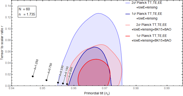
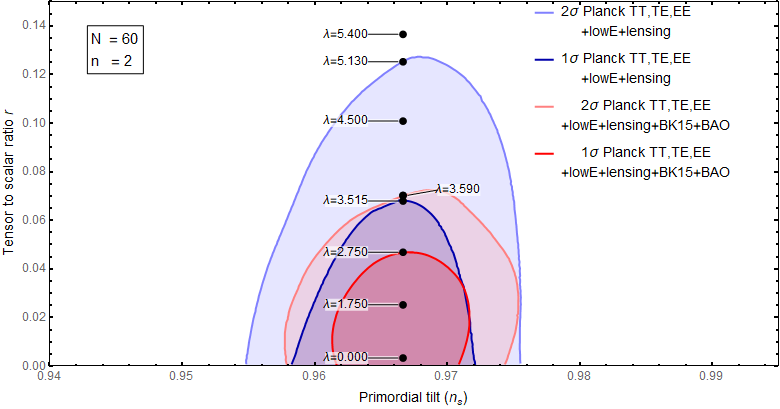
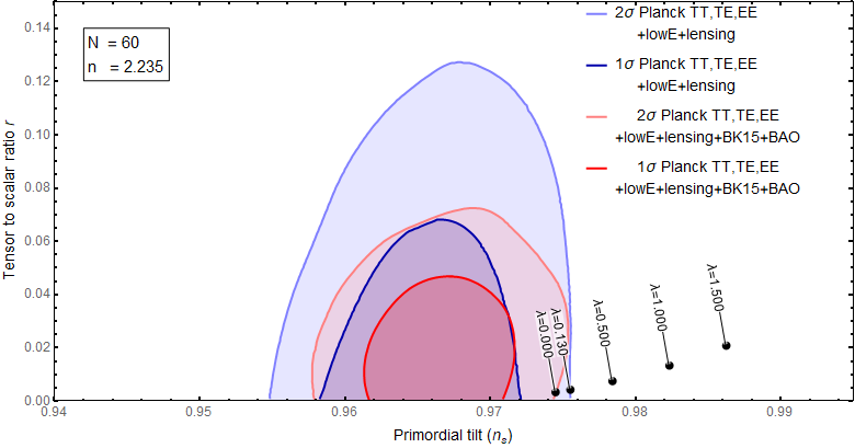
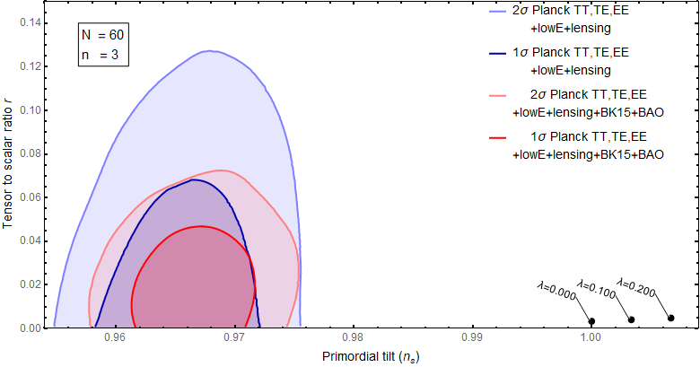
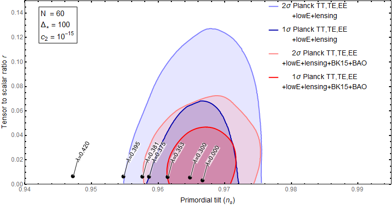
Figure 1: We compare the theoretical predictions in the (rns)𝑟subscript𝑛𝑠(r-n_{s}) plane for different values of λ𝜆\lambda using N=60𝑁60N=60 and varying n𝑛n. We plots for N=60,n=1.735formulae-sequence𝑁60𝑛1.735N=60,\,n=1.735 (upper-left panel); N=60,n=2formulae-sequence𝑁60𝑛2N=60,\,n=2 (upper-right panel); and for N=60,n=2.235formulae-sequence𝑁60𝑛2.235N=60,\,n=2.235 (lower-left panel); N=60,n=3formulae-sequence𝑁60𝑛3N=60,\,n=3 (lower-right panel) with Planck’15 results for TT, TE, EE, +lowE+lensing and +BK15+BAO.

We can further simplify the above result to yield

𝒫3n42n((HM)2+2λ)2nM24nπα(1+λ)2mP21(1+λ)2ϵ12,subscript𝒫superscript3𝑛superscript42𝑛superscriptsuperscript𝐻𝑀22𝜆2𝑛superscript𝑀24𝑛𝜋𝛼superscript1𝜆2superscriptsubscript𝑚P21superscript1𝜆2subscriptsuperscriptitalic-ϵ21\displaystyle\mathcal{P}_{\mathcal{R}}\approx\frac{3^{-n}4^{2-n}\left(\left(\frac{H}{M}\right)^{2+2\lambda}\right)^{2-n}M^{2}}{4n\pi\alpha(1+\lambda)^{2}m_{\rm P}^{2}}\frac{1}{(1+\lambda)^{2}\epsilon^{2}_{1}}\,, (4.13)

when we have inserted F(R)𝐹𝑅F(R) given in Eq.(4.11) into Eq.(4.12). It is worth noting that when n=2𝑛2n=2, we obtain a special case for which the Starobinky model is recovered. In this model, therefore, ϵ3subscriptitalic-ϵ3\epsilon_{3} reads

ϵ3=H˙(2λ+2(λ+1)n3)H2+H¨HH˙.subscriptitalic-ϵ3˙𝐻2𝜆2𝜆1𝑛3superscript𝐻2¨𝐻𝐻˙𝐻\displaystyle\epsilon_{3}=\frac{\dot{H}(-2\lambda+2(\lambda+1)n-3)}{H^{2}}+\frac{\ddot{H}}{H\dot{H}}\,. (4.14)

Assuming slow-roll approximations, the terms containing H¨¨𝐻\ddot{H} can be ignored and then the relation between ϵ3subscriptitalic-ϵ3\epsilon_{3} and ϵ1subscriptitalic-ϵ1\epsilon_{1} reads

ϵ3=ϵ1(2λ2(λ+1)n+3),subscriptitalic-ϵ3subscriptitalic-ϵ12𝜆2𝜆1𝑛3\displaystyle\epsilon_{3}=\epsilon_{1}(2\lambda-2(\lambda+1)n+3)\,, (4.15)

where we have used Eq.(4.8) and Eq.(4.27) together with Eq.(3.29). Hence, we have

n1subscript𝑛1\displaystyle n_{\mathcal{R}}-1 similar-to-or-equals\displaystyle\simeq 2(λ+2)ϵ1+2ϵ22ϵ3,2𝜆2subscriptitalic-ϵ12subscriptitalic-ϵ22subscriptitalic-ϵ3\displaystyle-2(\lambda+2)\epsilon_{1}+2\epsilon_{2}-2\epsilon_{3}\ , (4.16)
nsubscript𝑛\displaystyle n_{\mathcal{R}} =\displaystyle= 1+4ϵ1(λ(n2)+n3),14subscriptitalic-ϵ1𝜆𝑛2𝑛3\displaystyle 1+4\epsilon_{1}(\lambda(n-2)+n-3)\ , (4.17)

where we have defined a new parameter ΔH/MΔ𝐻𝑀\Delta\equiv H/M. For simplicity, let us suppose that during inflation the expansion is de Sitter (exponential) with a constant Hubble parameter. In terms of the number of efoldings, 𝒫,nsubscript𝒫subscript𝑛\mathcal{P}_{\mathcal{R}},\,n_{\mathcal{R}} and r𝑟r read

𝒫subscript𝒫\displaystyle\mathcal{P}_{\mathcal{R}} \displaystyle\approx 3n42n(Δ2+2λ)2nM2nπα(1+λ)2mP2N2(1+λ)2,superscript3𝑛superscript42𝑛superscriptsuperscriptΔ22𝜆2𝑛superscript𝑀2𝑛𝜋𝛼superscript1𝜆2superscriptsubscript𝑚P2superscript𝑁2superscript1𝜆2\displaystyle\frac{3^{-n}4^{2-n}\left(\Delta^{2+2\lambda}\right)^{2-n}M^{2}}{n\pi\alpha(1+\lambda)^{2}m_{\rm P}^{2}}\frac{N^{2}}{(1+\lambda)^{2}}, (4.18)
nsubscript𝑛\displaystyle n_{\mathcal{R}} \displaystyle\approx 16N+2nN4λN+2λnN,16𝑁2𝑛𝑁4𝜆𝑁2𝜆𝑛𝑁\displaystyle 1-\frac{6}{N}+\frac{2n}{N}-\frac{4\lambda}{N}+\frac{2\lambda n}{N}, (4.19)
r𝑟\displaystyle r \displaystyle\approx 12(λ+1)2N2.12superscript𝜆12superscript𝑁2\displaystyle\frac{12(\lambda+1)^{2}}{N^{2}}. (4.20)

We find that the above parameters reduce to those of the Starobinsky model when n=2,λ=0,α=1/6formulae-sequence𝑛2formulae-sequence𝜆0𝛼16n=2,\,\lambda=0,\,\alpha=1/6. We now compare our predicted results with Planck 2018 data. We find from Fig.(1) for N=60,n=1.735formulae-sequence𝑁60𝑛1.735N=60,\,n=1.735 that the predictions are consistent with the Planck’15 results for TT, TE, EE, +lowE+lensing at two sigma confidence level for 0.000λ0.3300.000𝜆0.3300.000\leq\lambda\leq 0.330 and lie outside the Planck’15 results for TT, TE, EE, +lowE+lensing+BK15+BAO for all values of λ𝜆\lambda. For N=60,n=2formulae-sequence𝑁60𝑛2N=60,\,n=2, our results are in excellent agreement with Planck’15 results for TT, TE, EE, +lowE+lensing and for TT, TE, EE, +lowE+lensing+BK15+BAO at one sigma confident level when 0.00λ3.5150.00𝜆3.5150.00\leq\lambda\leq 3.515 and 0.00λ2.7500.00𝜆2.7500.00\leq\lambda\leq 2.750, respectively.

Additionally, for N=60𝑁60N=60 and n=2.235𝑛2.235n=2.235, we discover that the predictions are consistent with the Planck’15 results for TT, TE, EE, +lowE+lensing at two sigma confidence level when 0.000λ0.1300.000𝜆0.1300.000\leq\lambda\leq 0.130 and lie at the boundary of the two sigma confident level when λ=0.00𝜆0.00\lambda=0.00. However, for N=60𝑁60N=60 and n=3𝑛3n=3, our results are inconsistent with Planck’15 results for TT, TE, EE, +lowE+lensing and TT, TE, EE, +lowE+lensing+BK15+BAO. Using Planck 2018 data for 𝒫subscript𝒫\mathcal{P}_{\mathcal{R}}, we can solve for n𝑛n to obtain

n𝑛\displaystyle n =\displaystyle= 4.76×10²(2.6738×10¹¹+5.34761×10¹¹λ+2.6738×10¹¹λ2)(1+λ)2(3.16388×10¹⁰+1.27324×10¹⁰Σ)×\displaystyle\frac{4.76\times 10^{-2}\left(2.6738\times 10^{11}+5.34761\times 10^{11}\lambda+2.6738\times 10^{11}\lambda^{2}\right)}{(1+\lambda)^{2}\left(3.16388\times 10^{10}+1.27324\times 10^{10}\,\Sigma\right)}\times (4.21)
×\displaystyle\times ProductLog[3.048×10²⁰N2Δ4λ(3.16×10¹⁰+1.27×10¹⁰Σ)αδ2(1+λ)2],ProductLogdelimited-[]3.048superscript1020superscript𝑁2superscriptΔ4𝜆3.16superscript10101.27superscript1010Σ𝛼superscript𝛿2superscript1𝜆2\displaystyle\text{ProductLog}\left[\frac{3.048\times 10^{-20}N^{2}\Delta^{4\lambda}\left(3.16\times 10^{10}+1.27\times 10^{10}\,\Sigma\right)}{\alpha\delta^{2}(1+\lambda)^{2}}\right],

where we have defined new parameters as

ΔH/M,δ=M/mP,Σlog[2.00×105Δ1+2λδ].formulae-sequenceΔ𝐻𝑀formulae-sequence𝛿𝑀subscript𝑚PΣ2.00superscript105superscriptΔ12𝜆𝛿\displaystyle\Delta\equiv H/M,\,\delta=M/m_{\rm P},\,\Sigma\equiv\log\left[\frac{2.00\times 10^{-5}\Delta^{1+2\lambda}}{\delta}\right]. (4.22)
Refer to caption
Refer to caption
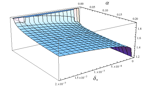
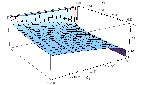
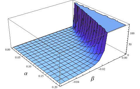
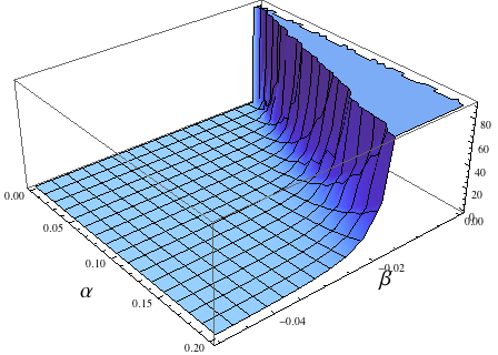
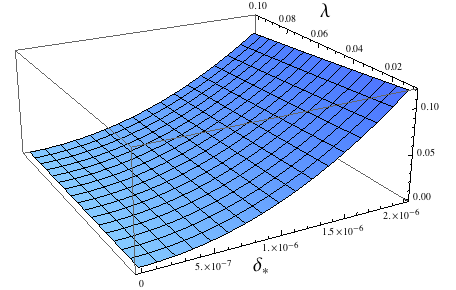
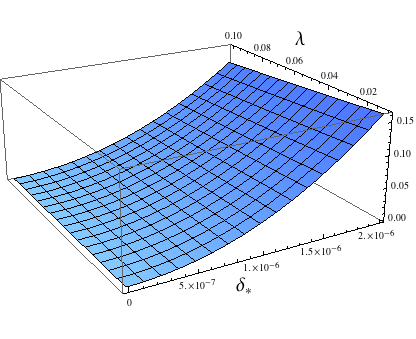
Figure 2: Figures show the behavior of n𝑛n against δsubscript𝛿\delta_{\star} and α𝛼\alpha given by Eq.(4.21). A vertical axis represents values of n𝑛n. For the plots we have used N=60𝑁60N=60 (left panel) and N=70𝑁70N=70 (right panel).

Having used an upper bound on the Hubble parameter during inflation observed by Planck, we can quantify how values of n𝑛n do depend on α𝛼\alpha and δsubscript𝛿\delta_{\star} during inflation. From Fig.2. we find the behavior of n𝑛n against δsubscript𝛿\delta_{\star} and α𝛼\alpha where we have used Δ=H/M,λ=0.1formulae-sequencesubscriptΔsubscript𝐻𝑀𝜆0.1\Delta_{\star}=H_{\star}/M,\,\lambda=0.1. Notice that

4.2 Model II: f(R)=R+αR2+βR2log(R/M2)𝑓𝑅𝑅𝛼superscript𝑅2𝛽superscript𝑅2𝑅superscript𝑀2f(R)=R+\alpha R^{2}+\beta R^{2}\log(R/M^{2})

In this second model, we consider a function f(R)𝑓𝑅f(R) of the form

f(R)=R+αR2+βR2log(R/M2).𝑓𝑅𝑅𝛼superscript𝑅2𝛽superscript𝑅2𝑅superscript𝑀2\displaystyle f(R)=R+\alpha R^{2}+\beta R^{2}\log(R/M^{2}). (4.23)

We can estimate F(R)=f(R)/dR𝐹𝑅𝑓𝑅𝑑𝑅F(R)=\partial f(R)/dR by assuming HMmuch-greater-than𝐻𝑀H\gg M during inflation to obtain

F(R)12H2(HM)2λ(2α+β+2βlog[12(HM)2+2λ]).𝐹𝑅12superscript𝐻2superscript𝐻𝑀2𝜆2𝛼𝛽2𝛽12superscript𝐻𝑀22𝜆\displaystyle F(R)\approx 12H^{2}\left(\frac{H}{M}\right)^{2\lambda}\left(2\alpha+\beta+2\beta\log\left[12\left(\frac{H}{M}\right)^{2+2\lambda}\right]\right). (4.24)

Considering Eq.(3.30), then the power spectrum of curvature perturbation reads

𝒫136πmP2(2α+β+2βlog[12(HM)2(1+λ)])1(1+λ)2ϵ12.subscript𝒫136𝜋superscriptsubscript𝑚P22𝛼𝛽2𝛽12superscript𝐻𝑀21𝜆1superscript1𝜆2subscriptsuperscriptitalic-ϵ21\displaystyle\mathcal{P}_{\mathcal{R}}\approx\frac{1}{36\pi m_{\rm P}^{2}\left(2\alpha+\beta+2\beta\log\left[12\left(\frac{H}{M}\right)^{2(1+\lambda)}\right]\right)}\frac{1}{(1+\lambda)^{2}\epsilon^{2}_{1}}\,. (4.25)

In this model, therefore, ϵ3subscriptitalic-ϵ3\epsilon_{3} reads

ϵ3=H˙(4αλ+2α+10βλ+7β+2(2βλ+β)log(12H2λ+2M2(λ+1)))H2(2α+3β+2βlog(12H2λ+2M2(λ+1)))+H¨HH˙.subscriptitalic-ϵ3˙𝐻4𝛼𝜆2𝛼10𝛽𝜆7𝛽22𝛽𝜆𝛽12superscript𝐻2𝜆2superscript𝑀2𝜆1superscript𝐻22𝛼3𝛽2𝛽12superscript𝐻2𝜆2superscript𝑀2𝜆1¨𝐻𝐻˙𝐻\displaystyle\epsilon_{3}=\frac{\dot{H}\left(4\alpha\lambda+2\alpha+10\beta\lambda+7\beta+2(2\beta\lambda+\beta)\log\left(12H^{2\lambda+2}M^{-2(\lambda+1)}\right)\right)}{H^{2}\left(2\alpha+3\beta+2\beta\log\left(12H^{2\lambda+2}M^{-2(\lambda+1)}\right)\right)}+\frac{\ddot{H}}{H\dot{H}}\,. (4.26)

Assuming slow-roll approximations, the terms containing H¨¨𝐻\ddot{H} can be ignored and then the relation between ϵ3subscriptitalic-ϵ3\epsilon_{3} and ϵ1subscriptitalic-ϵ1\epsilon_{1} reads

ϵ3=ϵ1(12λ4β(λ+1)2α+3β+2βlog(12M2λ2H(t)2λ+2)),subscriptitalic-ϵ3subscriptitalic-ϵ112𝜆4𝛽𝜆12𝛼3𝛽2𝛽12superscript𝑀2𝜆2𝐻superscript𝑡2𝜆2\displaystyle\epsilon_{3}=\epsilon_{1}\left(-1-2\lambda-\frac{4\beta(\lambda+1)}{2\alpha+3\beta+2\beta\log\left(12M^{-2\lambda-2}H(t)^{2\lambda+2}\right)}\right)\,, (4.27)

where we have used Eq.(4.8) and Eq.(4.27) together with Eq.(3.29). Hence, we have

n1subscript𝑛1\displaystyle n_{\mathcal{R}}-1 similar-to-or-equals\displaystyle\simeq 2(λ+2)ϵ1+2ϵ22ϵ3,2𝜆2subscriptitalic-ϵ12subscriptitalic-ϵ22subscriptitalic-ϵ3\displaystyle-2(\lambda+2)\epsilon_{1}+2\epsilon_{2}-2\epsilon_{3}\ , (4.28)
nsubscript𝑛\displaystyle n_{\mathcal{R}} =\displaystyle= 14ϵ1(2α2βλ+β+2βlog(12H2λ+2M2(λ+1)))2α+3β+2βlog(12H2λ+2M2(λ+1)),14subscriptitalic-ϵ12𝛼2𝛽𝜆𝛽2𝛽12superscript𝐻2𝜆2superscript𝑀2𝜆12𝛼3𝛽2𝛽12superscript𝐻2𝜆2superscript𝑀2𝜆1\displaystyle 1-\frac{4\epsilon_{1}\left(2\alpha-2\beta\lambda+\beta+2\beta\log\left(12H^{2\lambda+2}M^{-2(\lambda+1)}\right)\right)}{2\alpha+3\beta+2\beta\log\left(12H^{2\lambda+2}M^{-2(\lambda+1)}\right)}\ , (4.29)

where we have defined a new parameter ΔH/MΔ𝐻𝑀\Delta\equiv H/M. For simplicity, let us suppose that during inflation the expansion is de Sitter (exponential) with a constant Hubble parameter. In terms of the number of efoldings, 𝒫,nsubscript𝒫subscript𝑛\mathcal{P}_{\mathcal{R}},\,n_{\mathcal{R}} and r𝑟r read

𝒫subscript𝒫\displaystyle\mathcal{P}_{\mathcal{R}} \displaystyle\approx N29mP2π(1+λ)2(2α+β+2βLog[12(Δ)2(1+λ)])1,superscript𝑁29superscriptsubscript𝑚P2𝜋superscript1𝜆2superscript2𝛼𝛽2𝛽Logdelimited-[]12superscriptΔ21𝜆1\displaystyle\frac{N^{2}}{9m_{\rm P}^{2}\pi(1+\lambda)^{2}}\Big{(}2\alpha+\beta+2\beta\text{Log}\Big{[}12\left(\Delta\right)^{2(1+\lambda)}\Big{]}\Big{)}^{-1}, (4.30)
nsubscript𝑛\displaystyle n_{\mathcal{R}} \displaystyle\approx 12N+4β(λ+1)N(2α+2βlog(12Δ2λ+2)+3β),12𝑁4𝛽𝜆1𝑁2𝛼2𝛽12superscriptΔ2𝜆23𝛽\displaystyle 1-\frac{2}{N}+\frac{4\beta(\lambda+1)}{N\left(2\alpha+2\beta\log\left(12\Delta^{2\lambda+2}\right)+3\beta\right)}, (4.31)
r𝑟\displaystyle r \displaystyle\approx 12(λ+1)2N2.12superscript𝜆12superscript𝑁2\displaystyle\frac{12(\lambda+1)^{2}}{N^{2}}. (4.32)
Refer to caption
Refer to caption
Refer to caption
Refer to caption
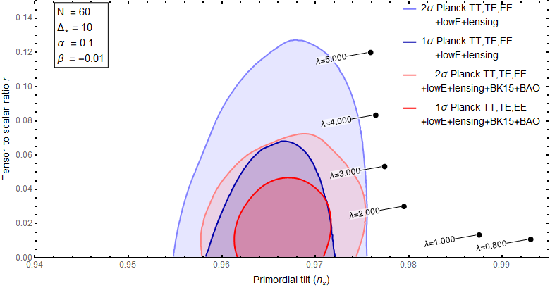
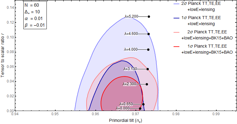
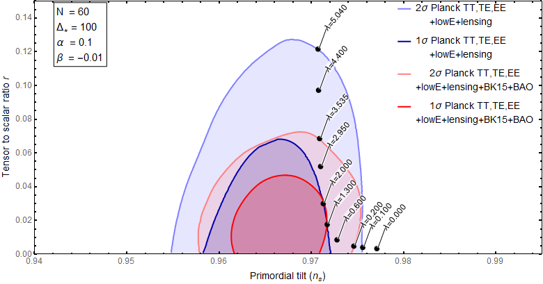
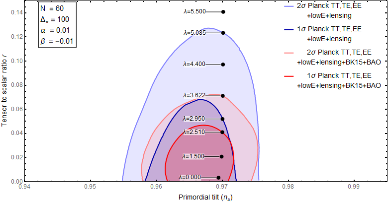
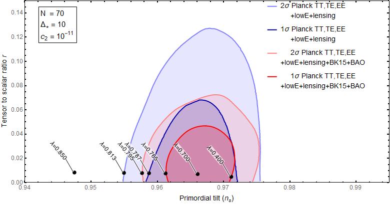
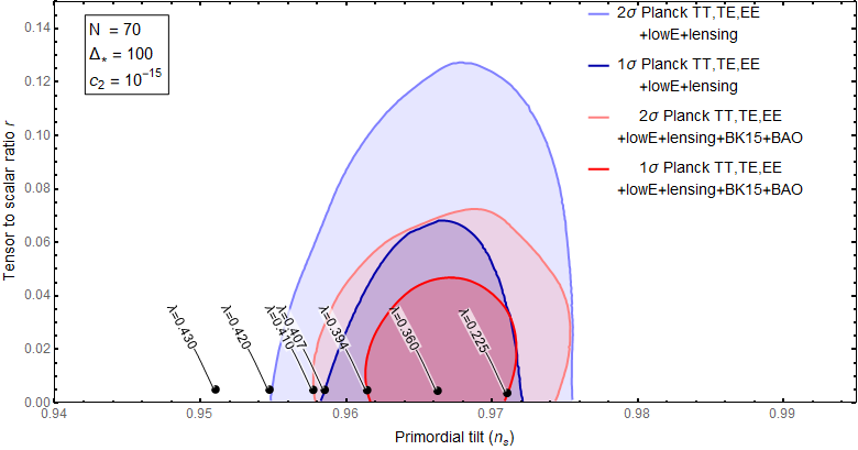
Figure 3: We compare the theoretical predictions in the (rns)𝑟subscript𝑛𝑠(r-n_{s}) plane for different values of λ𝜆\lambda using Δ=10, 100,α=0.1, 0.01,β=0.01,N=60formulae-sequencesubscriptΔ10100formulae-sequence𝛼0.10.01formulae-sequence𝛽0.01𝑁60\Delta_{\star}=10,\,100,\,\alpha=0.1,\,0.01,\,\beta=-0.01,\,N=60. (upper-left panel); Δ=100,α=0.01,β=0.01,N=60formulae-sequencesubscriptΔ100formulae-sequence𝛼0.01formulae-sequence𝛽0.01𝑁60\Delta_{\star}=100,\,\alpha=0.01,\,\beta=-0.01,\,N=60 (upper-right panel); Δ=10,α=0.1,β=0.01,N=60formulae-sequencesubscriptΔ10formulae-sequence𝛼0.1formulae-sequence𝛽0.01𝑁60\Delta_{\star}=10,\,\alpha=0.1,\,\beta=-0.01,\,N=60 (lower-left panel) and Δ=100,α=0.01,β=0.01,N=60formulae-sequencesubscriptΔ100formulae-sequence𝛼0.01formulae-sequence𝛽0.01𝑁60\Delta_{\star}=100,\,\alpha=0.01,\,\beta=-0.01,\,N=60 (lower-right panel) with Planck’15 results for TT, TE, EE, +lowE+lensing and +BK15+BAO.

We find that the above parameters reduce to those of the Starobinsky model when β=0=λ𝛽0𝜆\beta=0=\lambda. We now compare our predicted results with Planck 2018 data. We find from Fig.(3) for N=60𝑁60N=60 that the predictions are inconsistent with the Planck’15 results for TT, TE, EE, +lowE+lensing and +BK15+BAO at two sigma confidence level for Δ=10,α=0.1,β=0.01formulae-sequencesubscriptΔ10formulae-sequence𝛼0.1𝛽0.01\Delta_{\star}=10,\,\alpha=0.1,\,\beta=-0.01. However, the predictions lie well inside the two-sigma regions for Δ=10,α=0.01,β=0.01formulae-sequencesubscriptΔ10formulae-sequence𝛼0.01𝛽0.01\Delta_{\star}=10,\,\alpha=0.01,\,\beta=-0.01. Using Δ=100subscriptΔ100\Delta_{\star}=100, we discover that the results lie inside the two-sigma regions for α=0.1,β=0.01formulae-sequence𝛼0.1𝛽0.01\alpha=0.1,\,\beta=-0.01 and are in good agreement with TT, TE, EE, +lowE+lensing+BK15+BAO for α=0.01,β=0.01formulae-sequence𝛼0.01𝛽0.01\alpha=0.01,\,\beta=-0.01. We conclude that in order to have the predictions fit well inside the one-sigma regions of the Planck 2018 data we need either Δ𝒪(10)much-greater-thansubscriptΔ𝒪10\Delta_{\star}\gg{\cal O}(10) or α=|β|0.1𝛼𝛽much-less-than0.1\,\alpha=|\beta|\ll 0.1.

Additionally, for N=60𝑁60N=60, we discover that the predictions are in excellent agreement with consistent with the Planck’15 results for TT, TE, EE, +lowE+lensing and TT, TE, EE, +lowE+lensing and +BK15+BAO at one sigma confidence level for Δ=100, 0λ2.950formulae-sequencesubscriptΔ100 0𝜆2.950\Delta_{\star}=100,\,0\leq\lambda\leq 2.950 and Δ=100, 0λ2.510formulae-sequencesubscriptΔ100 0𝜆2.510\Delta_{\star}=100,\,0\leq\lambda\leq 2.510, respectively. Notice that when setting β=0𝛽0\beta=0, we clearly obtain the results of the Starobinsky model. Using Planck 2018 data for 𝒫subscript𝒫\mathcal{P}_{\mathcal{R}}, we can solve for ΔΔ\Delta to obtain

Δ=Exp[(β(1.141.14λ)3+α(0.790.79λ)3)β(1+λ)4+4.21×10⁶N2(1+λ)mP2β(1+λ)4],ΔExpdelimited-[]𝛽superscript1.141.14𝜆3𝛼superscript0.790.79𝜆3𝛽superscript1𝜆44.21superscript106superscript𝑁21𝜆superscriptsubscript𝑚P2𝛽superscript1𝜆4\displaystyle\Delta={\rm Exp}\Bigg{[}\frac{\Big{(}\beta(-1.14-1.14\lambda)^{3}+\alpha(-0.79-0.79\lambda)^{3}\Big{)}}{\beta(1+\lambda)^{4}}+\frac{4.21\times 10^{6}N^{2}(1+\lambda)}{m_{\rm P}^{2}\beta(1+\lambda)^{4}}\Bigg{]}, (4.33)
Refer to caption
Refer to caption
Figure 4: Figures show the behavior of ΔΔ\Delta against α𝛼\alpha and β𝛽\beta given by Eq.(4.33). A vertical axis represents values of ΔΔ\Delta. For the plots we have used N=60,λ=0.01formulae-sequence𝑁60𝜆0.01N=60,\,\lambda=0.01 (left panel) and N=60,λ=0.1formulae-sequence𝑁60𝜆0.1N=60,\,\lambda=0.1 (right panel).

It is worth noting that when β=0𝛽0\beta=0 a term ΔΔ\Delta disappears. We verify the behavior of ΔΔ\Delta during inflation as illustrated in Fig.4. From figures, we find that in order to obtain sizeable values of ΔsubscriptΔ\Delta_{\star}, e.g. Δ𝒪(10)𝒪(100)similar-tosubscriptΔ𝒪10𝒪100\Delta_{\star}\sim{\cal O}(10)-{\cal O}(100), we find that β𝛽\beta must be negative in a range 1.0β<0.1much-less-than1.0𝛽0.1-1.0\ll\beta<-0.1 together with α0.5much-less-than𝛼0.5\alpha\ll 0.5.

4.3 Model III: Einstein-Hu-Sawicki

In the last model, we consider the Hu-Sawicki model in which the f(R)𝑓𝑅f(R) function is of the form

f(R)=RM2c1(R/M2)nc2(R/M2)n+1,𝑓𝑅𝑅superscript𝑀2subscript𝑐1superscript𝑅superscript𝑀2𝑛subscript𝑐2superscript𝑅superscript𝑀2𝑛1\displaystyle f(R)=R-M^{2}\frac{c_{1}\Big{(}R/M^{2}\Big{)}^{n}}{c_{2}\Big{(}R/M^{2}\Big{)}^{n}+1}, (4.34)

where we have fixed n=2𝑛2n=2 in this present examination. Then F𝐹F defined by F(R)=f(R)/R𝐹𝑅𝑓𝑅𝑅F(R)=\partial f(R)/\partial R can be written by

F(R)=1+2c1c2R3M6(c2R2M4+1)22c1RM2(c2R2M4+1).𝐹𝑅12subscript𝑐1subscript𝑐2superscript𝑅3superscript𝑀6superscriptsubscript𝑐2superscript𝑅2superscript𝑀4122subscript𝑐1𝑅superscript𝑀2subscript𝑐2superscript𝑅2superscript𝑀41\displaystyle F(R)=1+\frac{2c_{1}c_{2}R^{3}}{M^{6}\left(\frac{c_{2}R^{2}}{M^{4}}+1\right)^{2}}-\frac{2c_{1}R}{M^{2}\left(\frac{c_{2}R^{2}}{M^{4}}+1\right)}. (4.35)

Therefore, ϵ3subscriptitalic-ϵ3\epsilon_{3} reads

ϵ3=H˙H2(12(λ+1)M4144c2H4(HM)4λ+M44(λ+1)M4M4432c2H4(HM)4λ6λ7)+H¨HH˙.subscriptitalic-ϵ3˙𝐻superscript𝐻212𝜆1superscript𝑀4144subscript𝑐2superscript𝐻4superscript𝐻𝑀4𝜆superscript𝑀44𝜆1superscript𝑀4superscript𝑀4432subscript𝑐2superscript𝐻4superscript𝐻𝑀4𝜆6𝜆7¨𝐻𝐻˙𝐻\displaystyle\epsilon_{3}=\frac{\dot{H}}{H^{2}}\left(\frac{12(\lambda+1)M^{4}}{144c_{2}H^{4}\left(\frac{H}{M}\right)^{4\lambda}+M^{4}}-\frac{4(\lambda+1)M^{4}}{M^{4}-432c_{2}H^{4}\left(\frac{H}{M}\right)^{4\lambda}}-6\lambda-7\right)+\frac{\ddot{H}}{H\dot{H}}\,. (4.36)

Assuming slow-roll approximations, the terms containing H¨¨𝐻\ddot{H} can be ignored and then the relation between ϵ3subscriptitalic-ϵ3\epsilon_{3} and ϵ1subscriptitalic-ϵ1\epsilon_{1} reads

ϵ3=ϵ1(12(λ+1)144c2(HM)4λ+4+1+4(λ+1)1432c2(HM)4λ+4+6λ+7),subscriptitalic-ϵ3subscriptitalic-ϵ112𝜆1144subscript𝑐2superscript𝐻𝑀4𝜆414𝜆11432subscript𝑐2superscript𝐻𝑀4𝜆46𝜆7\displaystyle\epsilon_{3}=\epsilon_{1}\left(-\frac{12(\lambda+1)}{144c_{2}\left(\frac{H}{M}\right)^{4\lambda+4}+1}+\frac{4(\lambda+1)}{1-432c_{2}\left(\frac{H}{M}\right)^{4\lambda+4}}+6\lambda+7\right)\,, (4.37)

where we have used Eq.(4.8) and Eq.(4.36) together with Eq.(3.29). Hence, we have

n1subscript𝑛1\displaystyle n_{\mathcal{R}}-1 similar-to-or-equals\displaystyle\simeq 2(λ+2)ϵ1+2ϵ22ϵ3,2𝜆2subscriptitalic-ϵ12subscriptitalic-ϵ22subscriptitalic-ϵ3\displaystyle-2(\lambda+2)\epsilon_{1}+2\epsilon_{2}-2\epsilon_{3}\ , (4.38)
nsubscript𝑛\displaystyle n_{\mathcal{R}} =\displaystyle= 12(λ+2)ϵ1+2(λ1)ϵ112𝜆2subscriptitalic-ϵ12𝜆1subscriptitalic-ϵ1\displaystyle 1-2(\lambda+2)\epsilon_{1}+2(-\lambda-1)\epsilon_{1} (4.39)
+2ϵ1(12(λ+1)144c2Δ4λ+4+14(λ+1)1432c2Δ4λ+46λ7),2subscriptitalic-ϵ112𝜆1144subscript𝑐2superscriptΔ4𝜆414𝜆11432subscript𝑐2superscriptΔ4𝜆46𝜆7\displaystyle+2\epsilon_{1}\left(\frac{12(\lambda+1)}{144c_{2}\Delta^{4\lambda+4}+1}-\frac{4(\lambda+1)}{1-432c_{2}\Delta^{4\lambda+4}}-6\lambda-7\right)\ ,

where we have defined a new parameter ΔH/MΔ𝐻𝑀\Delta\equiv H/M. For simplicity, let us suppose that during inflation the expansion is de Sitter (exponential) with a constant Hubble parameter. Here we assume that HH=constant𝐻subscript𝐻constantH\approx H_{\star}={\rm constant} and then define a new parameter Δ(H/M)subscriptΔsubscript𝐻𝑀\Delta_{\star}\equiv(H_{\star}/M) which is plausible during inflation. We consider Eq.(3.30) and then the power spectrum of curvature perturbation reads

𝒫1Qs(H2π)2(HM)2λ=13πF(HmP)2(HM)2λ1(1+λ)2ϵ12,subscript𝒫1subscript𝑄𝑠superscript𝐻2𝜋2superscript𝐻𝑀2𝜆13𝜋𝐹superscript𝐻subscript𝑚P2superscript𝐻𝑀2𝜆1superscript1𝜆2subscriptsuperscriptitalic-ϵ21\displaystyle\mathcal{P}_{\mathcal{R}}\approx\frac{1}{Q_{s}}\left(\frac{H}{2\pi}\right)^{2}\left(\frac{H}{M}\right)^{2\lambda}=\frac{1}{3\pi F}\left(\frac{H}{m_{\rm P}}\right)^{2}\left(\frac{H}{M}\right)^{2\lambda}\frac{1}{(1+\lambda)^{2}\epsilon^{2}_{1}}\,, (4.40)

when we have inserted Qssubscript𝑄𝑠Q_{s} defined in Eq.(4.2). We will see that c21very-much-less-thansubscript𝑐21c_{2}\lll 1 allowing to estimate F(R)2c1R/M2𝐹𝑅2subscript𝑐1𝑅superscript𝑀2F(R)\approx-2c_{1}R/M^{2} since RM2much-greater-than𝑅superscript𝑀2R\gg M^{2} during inflation. With this approximation, we find

𝒫172πc~1(MmP)21(1+λ)2ϵ12,subscript𝒫172𝜋subscript~𝑐1superscript𝑀subscript𝑚P21superscript1𝜆2subscriptsuperscriptitalic-ϵ21\displaystyle\mathcal{P}_{\mathcal{R}}\approx\frac{1}{72\pi{\tilde{c}_{1}}}\left(\frac{M}{m_{\rm P}}\right)^{2}\frac{1}{(1+\lambda)^{2}\epsilon^{2}_{1}}\,, (4.41)

where c~1=c1subscript~𝑐1subscript𝑐1{\tilde{c}_{1}}=-c_{1}. Furthermore, we can recall equation (3.42) and use equation (4.8) to find the tensor-to-scalar ratio r𝑟r:

r=48ϵ22=48(λ+1)2ϵ12.𝑟48superscriptsubscriptitalic-ϵ2248superscript𝜆12superscriptsubscriptitalic-ϵ12\displaystyle r=48\epsilon_{2}^{2}=48(\lambda+1)^{2}\epsilon_{1}^{2}. (4.42)

Now, we obtain the expressions of nsubscript𝑛n_{\mathcal{R}}, 𝒫subscript𝒫\mathcal{P}_{\mathcal{R}} and r𝑟r. Consequently. we can rewrite nsubscript𝑛n_{\mathcal{R}} and r𝑟r in terms of e-folds (N𝑁N) because it is convenient to constrain the predictions of our model. To do so, we can use the relation between ϵ1subscriptitalic-ϵ1\epsilon_{1} and N𝑁N given in Eq.(2.34) at the time for which a Hubble radius crossing. Therefore, 𝒫,nsubscript𝒫subscript𝑛\mathcal{P}_{\mathcal{R}},\,n_{\mathcal{R}} and r𝑟r read

𝒫subscript𝒫\displaystyle\mathcal{P}_{\mathcal{R}} \displaystyle\approx 118πc~1(MmP)2N2(1+λ)2,118𝜋subscript~𝑐1superscript𝑀subscript𝑚P2superscript𝑁2superscript1𝜆2\displaystyle\frac{1}{18\pi{\tilde{c}_{1}}}\left(\frac{M}{m_{\rm P}}\right)^{2}\frac{N^{2}}{(1+\lambda)^{2}}, (4.43)
nsubscript𝑛\displaystyle n_{\mathcal{R}} \displaystyle\approx 12λ+3N+1N(12(λ+1)144c2Δ4λ+4+14(λ+1)1432c2Δ4λ+46λ7),12𝜆3𝑁1𝑁12𝜆1144subscript𝑐2superscriptΔ4𝜆414𝜆11432subscript𝑐2superscriptΔ4𝜆46𝜆7\displaystyle 1-\frac{2\lambda+3}{N}+\frac{1}{N}\Bigg{(}\frac{12(\lambda+1)}{144c_{2}\Delta^{4\lambda+4}+1}-\frac{4(\lambda+1)}{1-432c_{2}\Delta^{4\lambda+4}}-6\lambda-7\Bigg{)}, (4.44)
r𝑟\displaystyle r \displaystyle\approx 12(λ+1)2N2.12superscript𝜆12superscript𝑁2\displaystyle\frac{12(\lambda+1)^{2}}{N^{2}}. (4.45)
Refer to caption
Refer to caption
Refer to caption
Refer to caption
Figure 5: We compare the theoretical predictions in the (rns)𝑟𝑛𝑠(r-ns) plane for different values of λ𝜆\lambda using Δ=10,c2=1011,N=60formulae-sequencesubscriptΔ10formulae-sequencesubscript𝑐2superscript1011𝑁60\Delta_{\star}=10,c_{2}=10^{-11},N=60 (upper-left panel); Δ=100,c2=1015,N=60formulae-sequencesubscriptΔ100formulae-sequencesubscript𝑐2superscript1015𝑁60\Delta_{\star}=100,c_{2}=10^{-15},N=60 (upper-right panel); Δ=10,c2=1011,N=70formulae-sequencesubscriptΔ10formulae-sequencesubscript𝑐2superscript1011𝑁70\Delta_{\star}=10,c_{2}=10^{-11},N=70 (lower-left panel) and Δ=100,c2=1015,N=70formulae-sequencesubscriptΔ100formulae-sequencesubscript𝑐2superscript1015𝑁70\Delta_{\star}=100,c_{2}=10^{-15},N=70 (lower-right panel) with Planck’15 results for TT, TE, EE, +lowE+lensing and +BK15+BAO.

We find that the above parameters reduce to those of the Starobinsky model when c2=0=λsubscript𝑐20𝜆c_{2}=0=\lambda. We now compare our predicted results with Planck 2018 data. We find from Fig.(5) for N=60𝑁60N=60 that the predictions are consistent with the Planck’15 results for TT, TE, EE, +lowE+lensing at two sigma confidence level for Δ=10(100),c2=1011(1015)formulae-sequencesubscriptΔ10100subscript𝑐2superscript1011superscript1015\Delta_{\star}=10(100),\,c_{2}=10^{-11}(10^{-15}) only when λ0.763(0.395)𝜆0.7630.395\lambda\leq 0.763(0.395) with Planck’15 results for TT, TE, EE, +lowE+lensing and with the Planck’15 results for TT, TE, EE, +lowE+lensing+BK15+BAO at two sigma confidence level for Δ=10(100),c2=1011(1015)formulae-sequencesubscriptΔ10100subscript𝑐2superscript1011superscript1015\Delta_{\star}=10(100),\,c_{2}=10^{-11}(10^{-15}) only when λ0.737(0.381)𝜆0.7370.381\lambda\leq 0.737(0.381). Additionally, for N=70𝑁70N=70, we discover that the predictions are consistent with the Planck’15 results for TT, TE, EE, +lowE+lensing at two sigma confidence level for Δ=10(100),c2=1011(1015)formulae-sequencesubscriptΔ10100subscript𝑐2superscript1011superscript1015\Delta_{\star}=10(100),\,c_{2}=10^{-11}(10^{-15}) only when λ0.813(0.420)𝜆0.8130.420\lambda\leq 0.813(0.420) with Planck’15 results for TT, TE, EE, +lowE+lensing and with the Planck’15 results for TT, TE, EE, +lowE+lensing+BK15+BAO at two sigma confidence level for Δ=10(100),c2=1011(1015)formulae-sequencesubscriptΔ10100subscript𝑐2superscript1011superscript1015\Delta_{\star}=10(100),\,c_{2}=10^{-11}(10^{-15}) only when λ0.795(0.410)𝜆0.7950.410\lambda\leq 0.795(0.410).

Interestingly, using an upper bound on the Hubble parameter during inflation reported by Planck 2018 [53] allows us to determine δ=M/mPsubscript𝛿𝑀subscript𝑚P\delta_{\star}=M/m_{\rm P}:

HmP=Δδ<2.5×10⁵(95%C.L.)δ<2.5Δ×105.\displaystyle\frac{H_{\star}}{m_{\rm P}}=\Delta_{\star}\delta_{\star}<2.5\times 10^{-5}\,(95\%\,C.L.)\,\,\rightarrow\,\,\delta_{\star}<\frac{2.5}{\Delta_{\star}}\times 10^{-5}. (4.46)

Using Planck 2018 data for 𝒫subscript𝒫\mathcal{P}_{\mathcal{R}}, we discover

c~13.53×10²²N2δ24.20×10¹⁵+8.40×10¹⁵λ+4.20×10¹⁵λ2.subscript~𝑐13.53superscript1022superscript𝑁2subscriptsuperscript𝛿24.20superscript10158.40superscript1015𝜆4.20superscript1015superscript𝜆2\displaystyle{\tilde{c}_{1}}\approx\frac{3.53\times 10^{22}\,N^{2}\delta^{2}_{\star}}{4.20\times 10^{15}+8.40\times 10^{15}\lambda+4.20\times 10^{15}\lambda^{2}}. (4.47)
Refer to caption
Refer to caption
Figure 6: Figures show the behavior of c~1subscript~𝑐1{\tilde{c}_{1}} against δsubscript𝛿\delta_{\star} and λ𝜆\lambda given by Eq.(4.47). A vertical axis represents values of c~1subscript~𝑐1{\tilde{c}_{1}}. For the plots we have used N=60𝑁60N=60 (left panel) and N=70𝑁70N=70 (right panel).

In order to figure out the behavior of c~1subscript~𝑐1{\tilde{c}_{1}}, we choose particular values of N𝑁N and λ𝜆\lambda and make plots displayed in Fig.6. We discover that in order to have parameter satisfying the Planck 2018 data, values of c~1subscript~𝑐1{\tilde{c}_{1}} is (much) less than unity for Δ=10(Δ=100)subscriptΔ10subscriptΔ100\Delta_{\star}=10\,(\Delta_{\star}=100). Interestingly, we can recover the predictions of the Starobinsky model, i.e. c~1=1/60.167subscript~𝑐1160.167{\tilde{c}_{1}}=1/6\approx 0.167, when λ1very-much-less-than𝜆1\lambda\lll 1.

5 Concluding remarks

In conclusion, we studied the f(R)𝑓𝑅f(R) models of inflation in the context of gravity’s rainbow theory. We have chosen three types of f(R)𝑓𝑅f(R) models: f(R)=R+α(R/M)n,f(R)=R+αR2+βR2log(R/M2)formulae-sequence𝑓𝑅𝑅𝛼superscript𝑅𝑀𝑛𝑓𝑅𝑅𝛼superscript𝑅2𝛽superscript𝑅2𝑅superscript𝑀2f(R)=R+\alpha(R/M)^{n},\,f(R)=R+\alpha R^{2}+\beta R^{2}\log(R/M^{2}) and the Einstein-Hu-Sawicki model with n,α,β𝑛𝛼𝛽n,\,\alpha,\,\beta being arbitrary real constants. Here R𝑅R and M𝑀M being the Ricci scalar and mass scale, respectively. For all models, the rainbow function is written in the power-law form of the Hubble parameter. We presented a detailed derivation of the spectral index of curvature perturbation and the tensor-to-scalar ratio and compared the predictions of our results with latest Planck 2018 data. With the sizeable number of e-foldings and proper choices of parameters, we discovered that the predictions of all f(R)𝑓𝑅f(R) models present in this work are in excellent agreement with the Planck analysis.

For f(R)=R+α(R/M)n𝑓𝑅𝑅𝛼superscript𝑅𝑀𝑛f(R)=R+\alpha(R/M)^{n} model, we discovered that values of n𝑛n cannot be any arbitrary. Using N=60𝑁60N=60, we observed that n=2.235𝑛2.235n=2.235 in order to have the results in agreement with the Planck 2018 data at the two sigma confident level. With f(R)=R+αR2+βR2log(R/M2)𝑓𝑅𝑅𝛼superscript𝑅2𝛽superscript𝑅2𝑅superscript𝑀2f(R)=R+\alpha R^{2}+\beta R^{2}\log(R/M^{2}), we conclude for N=60𝑁60N=60 that in order to have the predictions fit well inside the one-sigma regions of the Planck 2018 data we need either Δ𝒪(10)much-greater-thansubscriptΔ𝒪10\Delta_{\star}\gg{\cal O}(10) or α=|β|0.1𝛼𝛽much-less-than0.1\,\alpha=|\beta|\ll 0.1 and found that β𝛽\beta has to be negative. Having considered the last model, the Einstein-Hu-Sawicky gravity, we observed that with the sizeable number of e-foldings and proper choices of parameters our predictions are in good agreement with the Planck’15 results for TT, TE, EE, +lowE+lensing and +BK15+BAO. Last but not the least, regarding our present work, the effects of rainbow functions on the structure of compact objects are also worth investigating, see e.g. [65, 66].

Acknowledgments

The work of AW is financially supported by the Development and Promotion of Science and Technology Talents Project (DPST), the Institute for the Promotion of Teaching Science and Technology (IPST).

Appendix A Scalar (Ricci) curvature in gravity’ rainbow

It is rather straight forward to derive the Ricci scalar of the theory. Let us first consider the Ricci curvature Rμνsubscript𝑅𝜇𝜈R_{\mu\nu} and compute its R00subscript𝑅00R_{00}-component to obtain

R00=3(a¨ag~¨g~+a˙f~˙af~g~˙f~˙g~f~2a˙g~˙ag~+2(g~˙g~)2),subscript𝑅003¨𝑎𝑎¨~𝑔~𝑔˙𝑎˙~𝑓𝑎~𝑓˙˙~𝑔~𝑓~𝑔~𝑓2˙𝑎˙~𝑔𝑎~𝑔2superscript˙~𝑔~𝑔2\displaystyle R_{00}=-3\left(\frac{\ddot{a}}{a}-\frac{\ddot{\tilde{g}}}{\tilde{g}}+\frac{\dot{a}\dot{\tilde{f}}}{a\tilde{f}}-\frac{\dot{\dot{\tilde{g}}\tilde{f}}}{\tilde{g}\tilde{f}}-2\frac{\dot{a}\dot{\tilde{g}}}{a\tilde{g}}+2\left(\frac{\dot{\tilde{g}}}{\tilde{g}}\right)^{2}\right)\,, (A.1)

while the Riisubscript𝑅𝑖𝑖R_{ii}-component reads

Rii=aa˙f~f~˙+2a˙2f~2+aa¨f~2g~2a2f~f~˙g~˙+6aa˙f~2g~˙+a2f~2g~¨g~3+4a2f~2g~˙2g~4.subscript𝑅𝑖𝑖𝑎˙𝑎~𝑓˙~𝑓2superscript˙𝑎2superscript~𝑓2𝑎¨𝑎superscript~𝑓2superscript~𝑔2superscript𝑎2~𝑓˙~𝑓˙~𝑔6𝑎˙𝑎superscript~𝑓2˙~𝑔superscript𝑎2superscript~𝑓2¨~𝑔superscript~𝑔34superscript𝑎2superscript~𝑓2superscript˙~𝑔2superscript~𝑔4\displaystyle R_{ii}=\frac{a\dot{a}\tilde{f}\dot{\tilde{f}}+2\dot{a}^{2}\tilde{f}^{2}+a\ddot{a}\tilde{f}^{2}}{\tilde{g}^{2}}-\frac{a^{2}\tilde{f}\dot{\tilde{f}}\dot{\tilde{g}}+6a\dot{a}\tilde{f}^{2}\dot{\tilde{g}}+a^{2}\tilde{f}^{2}\ddot{\tilde{g}}}{\tilde{g}^{3}}+\frac{4a^{2}\tilde{f}^{2}\dot{\tilde{g}}^{2}}{\tilde{g}^{4}}\,. (A.2)

Clearly, when setting f~=1~𝑓1\tilde{f}=1 and g~=1~𝑔1\tilde{g}=1, the above results convert to those of the standard flat FLRW spacetime in the f(R)𝑓𝑅f(R) theory. The Ricci scalar R𝑅R con be simply extracted by contracting Rμνsubscript𝑅𝜇𝜈R_{\mu\nu} with gμνsubscript𝑔𝜇𝜈g_{\mu\nu} to obtain Ricci scalar

R=gμνRμν=6f~2(a¨a+a˙f~˙af~+a˙2a2)6f~2(g~¨g~+f~˙g~˙f~g~+4a˙g~˙ag~3g~˙2g~2).𝑅superscript𝑔𝜇𝜈subscript𝑅𝜇𝜈6superscript~𝑓2¨𝑎𝑎˙𝑎˙~𝑓𝑎~𝑓superscript˙𝑎2superscript𝑎26superscript~𝑓2¨~𝑔~𝑔˙~𝑓˙~𝑔~𝑓~𝑔4˙𝑎˙~𝑔𝑎~𝑔3superscript˙~𝑔2superscript~𝑔2\displaystyle R=g^{\mu\nu}R_{\mu\nu}=6\tilde{f}^{2}\left(\frac{\ddot{a}}{a}+\frac{\dot{a}\dot{\tilde{f}}}{a\tilde{f}}+\frac{\dot{a}^{2}}{a^{2}}\right)-6\tilde{f}^{2}\left(\frac{\ddot{\tilde{g}}}{\tilde{g}}+\frac{\dot{\tilde{f}}\dot{\tilde{g}}}{\tilde{f}\tilde{g}}+4\frac{\dot{a}\dot{\tilde{g}}}{a\tilde{g}}-3\frac{\dot{\tilde{g}}^{2}}{\tilde{g}^{2}}\right). (A.3)

References

  • [1] Cherenkov Telescope Array. (2020). Retrieved 13 April 2020, from https://www.cta-observatory.org/
  • [2] J. Magueijo and L. Smolin, Class. Quant. Grav.  21, 1725 (2004)
  • [3] Y. Ling, JCAP 0708, 017 (2007)
  • [4] Z. W. Feng and S. Z. Yang, Phys. Lett. B 772, 737 (2017)
  • [5] S. H. Hendi and M. Momennia, Phys. Lett. B 777, 222 (2018)
  • [6] S. Panahiyan, S. H. Hendi and N. Riazi, Nucl. Phys. B 938, 388 (2019)
  • [7] M. Dehghani, Phys. Lett. B 777 (2018) 351
  • [8] S. Upadhyay, S. H. Hendi, S. Panahiyan and B. Eslam Panah, PTEP 2018, no. 9, 093E01 (2018)
  • [9] M. Dehghani, Phys. Lett. B 785, 274 (2018)
  • [10] S. H. Hendi, A. Dehghani and M. Faizal, Nucl. Phys. B 914, 117 (2017)
  • [11] S. H. Hendi, S. Panahiyan, B. Eslam Panah, M. Faizal and M. Momennia, Phys. Rev. D 94, no. 2, 024028 (2016)
  • [12] S. H. Hendi, M. Faizal, B. E. Panah and S. Panahiyan, Eur. Phys. J. C 76, no. 5, 296 (2016)
  • [13] S. H. Hendi and M. Faizal, Phys. Rev. D 92, no. 4, 044027 (2015)
  • [14] A. F. Ali, M. Faizal, B. Majumder and R. Mistry, Int. J. Geom. Meth. Mod. Phys.  12, no. 09, 1550085 (2015)
  • [15] A. F. Ali, M. Faizal and M. M. Khalil, Nucl. Phys. B 894, 341 (2015)
  • [16] A. F. Ali, M. Faizal and M. M. Khalil, Phys. Lett. B 743, 295 (2015)
  • [17] A. F. Ali, M. Faizal and M. M. Khalil, JHEP 1412, 159 (2014)
  • [18] A. F. Ali, M. Faizal and B. Majumder, EPL 109, no. 2, 20001 (2015)
  • [19] B. Eslam Panah, Phys. Lett. B 787, 45 (2018)
  • [20] Z. W. Feng, S. Z. Yang, H. L. Li and X. T. Zu, arXiv:1608.06824 [physics.gen-ph].
  • [21] S. H. Hendi, S. Panahiyan, S. Upadhyay and B. Eslam Panah, Phys. Rev. D 95, no. 8, 084036 (2017)
  • [22] D. Momeni, S. Upadhyay, Y. Myrzakulov and R. Myrzakulov, Astrophys. Space Sci.  362, no. 9, 148 (2017)
  • [23] X. M. Deng and Y. Xie, Phys. Lett. B 772, 152 (2017)
  • [24] M. Khodadi, K. Nozari and B. Vakili, Gen. Rel. Grav.  48, no. 5, 64 (2016)
  • [25] M. Khodadi, K. Nozari and H. R. Sepangi, Gen. Rel. Grav.  48, no. 12, 166 (2016)
  • [26] P. Rudra, M. Faizal and A. F. Ali, Nucl. Phys. B 909, 725 (2016)
  • [27] A. Ashour, M. Faizal, A. F. Ali and F. Hammad, Eur. Phys. J. C 76, no. 5, 264 (2016)
  • [28] R. Garattini, JCAP 1306, 017 (2013)
  • [29] R. Garattini and E. N. Saridakis, Eur. Phys. J. C 75, no. 7, 343 (2015)
  • [30] S. H. Hendi, M. Momennia, B. Eslam Panah and M. Faizal, Astrophys. J.  827, no. 2, 153 (2016)
  • [31] S. H. Hendi, M. Momennia, B. Eslam Panah and S. Panahiyan, Phys. Dark Universe 16 (2017) 26
  • [32] Y. Heydarzade, P. Rudra, F. Darabi, A. F. Ali and M. Faizal, Phys. Lett. B 774, 46 (2017)
  • [33] S. H. Hendi, B. Eslam Panah, S. Panahiyan and M. Momennia, Adv. High Energy Phys.  2016, 9813582 (2016)
  • [34] A. Chatrabhuti, V. Yingcharoenrat and P. Channuie, Phys. Rev. D 93, no. 4, 043515 (2016)
  • [35] A. Codello, J. Joergensen, F. Sannino and O. Svendsen, JHEP 1502, 050 (2015)
  • [36] P. Channuie, Eur. Phys. J. C 79 (2019) no.6, 508
  • [37] S. Nojiri and S. D. Odintsov, Phys. Rept.  505, 59 (2011)
  • [38] S. Nojiri, S. D. Odintsov and V. K. Oikonomou, Phys. Rept.  692, 1 (2017)
  • [39] T. P. Sotiriou and V. Faraoni, Rev. Mod. Phys.  82, 451 (2010)
  • [40] A. De Felice and S. Tsujikawa, Living Rev. Rel.  13, 3 (2010)
  • [41] S. Nojiri and S. D. Odintsov, Gen. Rel. Grav. 36 (2004), 1765-1780
  • [42] E. Elizalde, S. Odintsov, V. Oikonomou and T. Paul, JCAP 02 (2019), 017
  • [43] M. F. Shamir and I. Fayyaz, Mod. Phys. Lett. A 35 (2019) no.02, 1950354
  • [44] J. Sadeghi and H. Farahani, Phys. Lett. B 751 (2015), 89-95
  • [45] W. Hu and I. Sawicki, Phys. Rev. D 76, 064004 (2007)
  • [46] B. Hu, M. Raveri, M. Rizzato and A. Silvestri, Mon. Not. Roy. Astron. Soc.  459, no. 4, 3880 (2016)
  • [47] Y. Akrami et al. [Planck Collaboration], arXiv:1807.06211 [astro-ph.CO].
  • [48] A. A. Starobinsky, Phys. Lett. B 91, 99 (1980)
  • [49] G. Amelino-Camelia, Phys. Lett. B 510, 255 (2001)
  • [50] G. Amelino-Camelia, Int. J. Mod. Phys. D 11 (2002) 35
  • [51] G. Amelino-Camelia, J. Kowalski-Glikman, G. Mandanici and A. Procaccini, Int. J. Mod. Phys. A 20 (2005) 6007
  • [52] P. A. R. Ade et al. [Planck Collaboration], Astron. Astrophys.  594, A20 (2016)
  • [53] Y. Akrami et al. [Planck Collaboration], arXiv:1807.06211 [astro-ph.CO].
  • [54] A. A. Starobinsky, Phys. Lett. B 91, 99 (1980) [Phys. Lett.  91B, 99 (1980)] [Adv. Ser. Astrophys. Cosmol.  3, 130 (1987)]
  • [55] L. Sebastiani, G. Cognola, R. Myrzakulov, S. D. Odintsov and S. Zerbini, Phys. Rev. D 89, no. 2, 023518 (2014)
  • [56] A. de la Cruz-Dombriz, E. Elizalde, S. D. Odintsov and D. Sáez-Gómez, JCAP 1605, no. 05, 060 (2016)
  • [57] E. Elizalde, S. D. Odintsov, T. Paul and D. Sáez-Chillón Gómez, Phys. Rev. D 99, no. 6, 063506 (2019)
  • [58] S. D. Odintsov and V. K. Oikonomou, Annals Phys.  388, 267 (2018)
  • [59] I. G. Avramidi, Lect. Notes Phys. Monogr.  64, 1 (2000)
  • [60] A. Nishizawa and H. Motohashi, Phys. Rev. D 89, no. 6, 063541 (2014)
  • [61] D. Baumann et al. [CMBPol Study Team], AIP Conf. Proc. 1141 (2009) no.1, 10-120
  • [62] P. André et al. [PRISM], JCAP 02 (2014), 006
  • [63] F. Finelli et al. [CORE], JCAP 04 (2018), 016
  • [64] L. Verde, H. Peiris and R. Jimenez, JCAP 01 (2006), 019
  • [65] B. Eslam Panah, G. H. Bordbar, S. H. Hendi, R. Ruffini, Z. Rezaei and R. Moradi, Astrophys. J.  848, no. 1, 24 (2017)
  • [66] S. H. Hendi, G. H. Bordbar, B. E. Panah and S. Panahiyan, JCAP 1609, no. 09, 013 (2016)