A Practical Algorithm for the Computation of the Genus

Abstract

We describe a practical algorithm to compute the (oriented) genus of a graph, give results of the program implementing this algorithm, and compare the performance to existing algorithms. The aim of this algorithm is to be fast enough for many applications instead of focusing on the theoretical asymptotic complexity.
Apart from the specific problem and the results, the article can also be seen as an example how some design principles used to carefully develop and implement standard backtracking algorithms can still result in very competitive programs.

Keywords: genus, NP-complete, backtracking

1 Introduction

Algorithms are studied in two different ways. The first one is as underlying methods of computer programs. These algorithms only come to their right when implemented as a program and used as a tool. The second way is as objects of research themselves. In this case the emphasis lies on determining the asymptotic complexity of a problem – that is: of optimal algorithms solving the problem – often without the intention or realistic possibility to transform the described algorithms to a computer program that can be used. Even if such algorithms could be implemented and used, many would be extremely inefficient for real problem sizes and outperform standard algorithms only for problem sizes far beyond the limit where either of them can be used. Of course there are also some nice cases – e.g. the linear time planarity algorithm described in [3] – where both aspects meet and algorithms with the best asymptotic behaviour also perform well in practice.

The general difference between these two approaches can very well be illustrated at the example of the problem of determining the genus of a graph, which is defined as the genus of the smallest orientable 2-manifold so that the graph can be embedded on its surface without crossing edges. The problem is NP-complete [13], but for any fixed $g$ there is a linear time algorithm that can compute the genus $g^{\prime}\leq g$ or decide that it has genus larger than $g$ [11]. On the other hand, there is no algorithm implemented and available that is at least guaranteed to compute the genus of a single sparse graph with, say, 80 vertices, or determine that it has genus larger than 20, in one year of CPU time.

Even lately papers have been published that theoretically determine the genus of specific relatively small graphs or describe algorithms fine tuned for these graphs [6][7][9], but in addition to that, researchers have also started to develop general purpose genus computation programs. In [1] such an algorithm based on an integer linear programming approach was published. Later, an improved approach described in [5] was – although also being a general purpose algorithm – able to achieve many of the results formerly obtained by individual research, automatically in a reasonable amount of time. Unfortunately these programs are neither publicly available nor easy to use.

In this article we will describe an algorithm that – in spite of also being exponential already for small genus – clearly outperforms these approaches and is widely usable. The program based on this algorithm has the options to compute the genus of a graph, one or all minimum genus embeddings, one or all embeddings on an orientable surface of given genus, or to filter large lists of graphs for those with genus at most or at least a given bound. When choosing for all embeddings, for graphs with a nontrivial symmetry group isomorphic embeddings can be generated, but no two embeddings that are (labelled) mirror images are generated. We use a carefully designed backtracking algorithm.

2 The algorithm

We assume all input graphs to be simple connected graphs. The embeddings are constructed by interpreting each undirected edge as a pair of oppositely directed edges. We build a rotation system, that is a cyclic ordering of all directed edges starting in a vertex and interpret this ordering as clockwise. Faces of an embedded graph are defined by the usual face tracing algorithm starting from a directed edge $(v,w)$ and constructing the face containing $(v,w)$ by going to the inverse edge $(w,v)$, and then to the next edge in the orientation around $w$. This process is repeated until being back at $(v,w)$. A face $f$ is thus a set of oriented edges. The set of all vertices contained in one of the directed edges of a face $f$ will be denoted by $f^{v}$, $f(e)$ will denote the number of directed edges in the face containing the directed edge $e$, $F$ will denote the set of all such faces, $V$ the set of vertices, and $E$ the set of edges. The genus $g$ of the embedded graph is $g=1+(|E|-|V|-|F|)/2$.

Preprocessing:

Vertices of degree $1$ are irrelevant when computing the genus – they can simply be removed without any impact on the genus. Similarly vertices of degree $2$ can be replaced by an edge connecting their two neighbours. If this operation produces a double edge, the new edge can be removed too without changing the genus of the graph. Except when all embeddings of a graph on a certain genus must be computed and there are at least three vertices, these operations are recursively applied before the real computation of the genus begins. This means that e.g. cycles, trees or complete bipartite graphs $K_{2,n}$ are all reduced to a single vertex. After having computed an embedding, reduced vertices are restored. For graphs with minimum degree at least $3$ – which is almost always the case when mathematical research about the genus is done – this preprocessing step has of course no impact.

When computing the genus, the algorithm works by first searching for plane embeddings, then embeddings with genus 1, etc. until an embedding is found. The upper bound for the genus of the embedding that is to be constructed is used in the recursive routine embedding edges. When trying to embed the graph in genus $g>0$, it has already been determined that there are no embeddings of genus at most $g-1$ and the first embedding of genus $g$ determines the genus of the graph. Sometimes – this also depends on chance – such an embedding can be found relatively fast and the real bottleneck is the complete search for embeddings of genus $g-1$. By computing a lower bound on the genus, sometimes expensive complete searches can be avoided, but the lower bound must be fast to compute in order to have an advantage over the complete search. We will now first describe a method to compute a (cheap) lower bound:

Computing a lower bound for the genus:

When embedding a graph $G=(V,E)$, the values of $|V|$ and $|E|$ are fixed, so a minimum genus embedding is in fact an embedding with a maximum number of faces and if $f^{\prime}$ is an upper bound on the number of faces in any embedding then $g^{\prime}=\lceil 1+\frac{|E|-|V|-f^{\prime}}{2}\rceil$ is a lower bound on the genus.

A trivial upper bound on the number of faces is $\frac{2|E|}{3}$ as all faces have at least three edges. This lower bound is practically free and is always computed and used. Instead of the constant value $3$, except for trees one could also use the girth of the graph, but tat would also have to be computed. The following methods give a better bound if there are few cycles of minimum length.

For a given embedding, let $s[]$ denote the vector of size $2|E|$ indexed from 1 to $2|E|$ containing all values $f(e)$ of directed edges $e$ in non-decreasing order. Then $|F|=F(s)=\sum_{i=1}^{2|E|}(1/s[i])$. A vector $s^{\prime}[]$ of size $2|E|$ with $s^{\prime}[i]\leq s[i]$ for $1\leq i\leq 2|E|$, is said to be dominated by $s[]$. For a vector $s^{\prime}[]$ dominated by $s[]$ we have $F(s^{\prime})=\sum_{i=1}^{2|E|}(1/s^{\prime}[i])\geq f$.

We call a cyclic sequence $e_{0},\dots,e_{k-1}$ of $k$ pairwise distinct directed edges a facial-like walk if and only if for $0\leq i<k$ the starting vertex of $e_{i+1\ (\mathrm{mod}\ k)}$ is the end vertex of $e_{i}$ and $e_{i+1\ (\mathrm{mod}\ k)}$ is the inverse $(e_{i})^{-1}$ of $e_{i}$ if and only if the degree of the end vertex of $e_{i}$ is one. A first approximation $s_{0}[]$ of $s[]$ is obtained by taking for each directed edge $e$ the length $f_{w}(e)$ of the shortest facial-like walk containing $e$. The value of $f_{w}(e)$ can be easily computed by a Breadth First Search.

As each facial walk in an embedded graph is also a facial like walk, we see immediately that the non-decreasing sequence $s_{0}[]$ is dominated by $s[]$, as $f_{w}(e)\leq f(e)$ for each directed edge $e$. Especially $s_{0}[2|E|]\leq s[2|E|]$ and as in $s[]$ at least $s[2|E|]$ edges – all directed edges in a longest facial walk – have value $s[2|E|]$, we can replace the last $s_{0}[2|E|]$ values of $s_{0}[]$ with $s_{0}[2|E|]$ and get another sequence $s_{1}[]$ dominated by $s[]$. We use $F(s_{1})$ as a first nontrivial upper bound on the number of faces.

In fact the length of the shortest facial-like walk is the same for a directed edge and its reverse, but unless the graph is a cycle, one facial-like walk that does not also contain the reverse edge, can only form a face for at most one of them. This observation might lead to a better approximation, but in order to keep the computation of the approximation easy and fast, the length of the shortest facial-like walk is used for a directed edge and its inverse.

An angle $\alpha$ of a face is a pair of directed edges, following each other in the facial walk. The central vertex of the angle is the endpoint of the first edge – so except when this vertex has degree $1$ it is the only common vertex of the two edges. In what follows we use that for an edge $e$ and its inverse $e^{-1}$ we have $f_{w}(e)=f_{w}(e^{-1})$.

Instead of summing over all edges, we can sum over all angles. With $f(\alpha)$ the size of the face that contains $\alpha$ and $A(v)$ the set of all angles with central vertex $v$, we have $|F|=\sum_{v\in V}(\sum_{\alpha\in A(v)}1/f(\alpha))$. If for a vertex $v$ the sequence $s^{\prime}_{v}[1],\dots,s^{\prime}_{v}[\deg(v)]$ is the non-decreasing sequence of all $f(\alpha)$ with $\alpha\in A(v)$, then $|F|=\sum_{v\in V}(\sum_{1\leq i\leq\deg(v)}1/s^{\prime}_{v}[i])$. Taking for each vertex $v$ a vector dominated by $s^{\prime}_{v}[]$ we again get an upper bound on $|F|$. If we take for a vertex $v$ and each angle $\alpha\in A(v)$ instead of $f(\alpha)$ the value $\max\{f_{w}(e),f_{w}(e^{\prime})\}$, with $e,e^{\prime}$ the edges in the angle, we get a non-decreasing sequence $s^{\prime}_{0,v}[]$ dominated by $s^{\prime}_{v}[]$. If $s^{\prime}_{1,v}[]$ is the non-decreasing sequence of values of $f_{w}(e)$ with $e$ starting at $v$, then we define $s^{\prime}_{2,v}[]=s^{\prime}_{1,v}[2],s^{\prime}_{1,v}[3],\dots,s^{\prime}_{1,v}[\deg(v)],s^{\prime}_{1,v}[\deg(v)]$. So we remove the smallest value of $s^{\prime}_{1,v}[]$ and add a copy of the largest value.

Remark 2.1

Let $G=(V,E)$ be an embedded graph. Then for each vertex $v\in V$ the sequence $s^{\prime}_{v}[]$ dominates $s^{\prime}_{2,v}[]$.

Proof:

We know that $s^{\prime}_{v}[]$ dominates $s^{\prime}_{0,v}[]$. We will show that $s^{\prime}_{0,v}[]$ dominates $s^{\prime}_{2,v}[]$. As the maximum values of $s^{\prime}_{0,v}[]$, $s^{\prime}_{1,v}[]$ and $s^{\prime}_{2,v}[]$ are the same, it is sufficient to prove $s^{\prime}_{0,v}[i]\geq s^{\prime}_{2,v}[i]=s^{\prime}_{1,v}[i+1]$ for $i<\deg(v)$. Let $\alpha_{1},\dots,\alpha_{i}$ be the angles (that is: pairs of edges) determining the values $s^{\prime}_{0,v}[1],\dots,s^{\prime}_{0,v}[i]$ and $S_{i,v}$ be the set of all directed edges starting at $v$, so that $e$ or $e^{-1}$ is in at least one of these angles. Then the value of $s^{\prime}_{0,v}[i]$ is $\max\{f_{w}(e)|e\in S_{i,v}\}$ (here we use that $f_{w}(e)=f_{w}(e^{-1})$) and as $|S_{i,v}|\geq i+1$, we have that $s^{\prime}_{0,v}[i]\geq s^{\prime}_{1,v}[i+1]$.

 

We use $\sum_{v\in V}(\sum_{1\leq i\leq\deg(v)}1/s^{\prime}_{2,v}[i])$ as a second nontrivial upper bound on the number of faces.

These upper bounds on the number of faces and the corresponding lower bounds on the genus are relatively fast to compute. Nevertheless they do not always speed up the program. Especially for small graphs or small genus they can even slow down the program, as the embedding algorithm can exclude low genus embeddings very fast. While for few small graphs this is no problem, for large lists of small graphs it can be a problem. Of course the bounds can never slow down the program much, but can speed it up a lot:

In this article, all running times for the C-program multi_genus implementing the algorithm described here are on an Intel Core i7-9700 CPU @ 3.00GHz (running on one core at 4.4-4.7 Ghz). Examples for the impact of the computation of a lower bound when computing the genera of graphs are:

All bipartite graphs on 14 vertices with degrees between 5 and 6 (73 graphs, genus 3 to 5): without lower bound 60.9 seconds, with lower bound 0.035 seconds.
All cubic graphs on 22 vertices (7,319,447 graphs, genus 0 to 3): without lower bound 300 seconds, with lower bound 364 seconds.
Checking 1,000,000 random cubic graphs on 50 vertices, generated by genrang (which is part of the nauty-package [10]) for being planar: without lower bound 18.5 seconds, with lower bound 56.2 seconds.
Checking the same 1,000,000 random cubic graphs on 50 vertices for having genus at most $1$: without lower bound 144.8 seconds, with lower bound 85.5 seconds.

The default is that the nontrivial bounds are used, but the use can be switched off by an option to multi_genus.

Constructing an embedding

We begin by relabeling the graph in a BFS way. The time necessary to compute the genus can differ a lot for isomorphic graphs depending on the labelling. In some cases a BFS labelling results in a better performance, in others it slows down the program. We have chosen for the BFS labeling as the results for different, but isomorphic, input graphs often differ less when always using such a labeling. An example showing the large differences that can still occur can be seen when computing a genus 7 embedding (that is a minimum genus embedding) of $C_{3}\square C_{3}\square C_{3}$. Taking the first graph of the file ucay27_05_k=06 provided by Gordon Royle in his list of Cayley graphs (and doing BFS), it takes $0.19$ seconds to find an embedding, taking the same graph from a program constructing cartesian products and not doing BFS, it takes $6.2$ seconds. Taking the graph from the second source and doing BFS, it takes $281$ seconds. So even when relabeling the graph in a BFS manner the time still depends on the labeling of the input graph.

The algorithm works by first greedily embedding a subgraph so that for each embedding or its mirror image, the induced embedding of this subgraph is the one constructed. It has genus $0$. Then we add one edge at a time to the embedding. If the maximum degree is smaller than $3$, the graph is a path or a cycle, both of which can be uniquely embedded and only in the plane. Otherwise we construct the initial subgraph by taking a vertex with minimum degree among all vertices with degree at least $3$, embedding this vertex and three of its edges in an arbitrary way (thereby fixing the orientation) and greedily extending the three edges – one after the other – to paths until they cannot be made longer. The result of this construction forms the root of the recursion tree.

In branch and bound algorithms, the performance is often improved if one manages to reduce the branching at every node of the recursion tree. This is not a mathematical theorem, but more a rule of thumb, as in some cases more branching might be beneficial if it allows earlier bounding. Nevertheless in our case we have chosen to take small branching as the base (but not only) criterion for the order in which the edges are inserted. As an expensive choice of the next edge to insert is sometimes more costly than more branching, we work in three parts:

(i)

Before the recursion starts, the edges that are still to be embedded are sorted as $\{x_{1},y_{1}\},\dots,\{x_{k},y_{k}\}$, so that with $S_{i}$ the initial subgraph with edges $\{x_{1},y_{1}\},\dots,\{x_{i},y_{i}\}$ added, for $1\leq i<k$, we have for $\{x_{i},y_{i}\}$ that at least one of $x_{i},y_{i}$ is in $S_{i}$ and $\deg_{S_{i-1}}(x_{i})\cdot\deg_{S_{i-1}}(y_{i})\leq\deg_{S_{i-1}}(x_{j})\cdot\deg_{S_{i-1}}(y_{j})$ for all $i<j\leq k$ for which at least one of $x_{j},y_{j}$ is in $S_{i}$. If one of $\deg_{S_{i-1}}(x_{i}),\deg_{S_{i-1}}(y_{i})$ is $0$, then also $\deg_{S_{i-1}}(x_{i})+\deg_{S_{i-1}}(y_{i})\leq\deg_{S_{i-1}}(x_{j})+\deg_{S_{i-1}}(y_{j})$ for all $j$ for which one of $deg_{S_{i-1}}(x_{j}),\deg_{S_{i-1}}(y_{j})$ is $0$ and the other is in $S_{i}$. Informally speaking: first all edges leading from the already embedded part to not yet included vertices are added and then the edges with both endpoints in the embedded subgraph are added. In each case we choose an edge that has the smallest number of possibilities how it can be added if there are no other restrictions.

During the recursion we always have an upper bound max_genus on the genus. As long as this bound is not reached, edges can be inserted in all possible angles – sometimes increasing the genus and sometimes not. In order to reach this bound as fast as possible and therefore be able to reduce the branching, we check at each node of the recursion tree whether there is an edge that cannot be embedded in any existing face of the partial embedding – we call such an edge a critical edge – and therefore always increases the genus. If there is such an edge and the partial embedding has already genus max_genus, we can backtrack, otherwise the first such edge in the list gets priority above other edges that do not have this property and is inserted first.

We distinguish two cases:

(ii)

If the recursion is still close to the root node and the genus of the partial embedding is still smaller than max_genus, we have relatively few nodes and the impact of a smaller branching is large. In this situation, also more expensive tests can pay and we do not only check for the existence of a critical edge, but do in fact look for an edge which has the smallest number of faces into which it can be embedded and take such an edge as the next one to be embedded. Among all edges with the same number of faces where they can be embedded, the first one in the sorted list is taken. Note that it is possible that an edge can be embedded into a face in more than one way, but this is not taken into account when counting the number of faces.

(iii)

Close to the leaves of the recursion tree we have many nodes and the impact of a smaller branching is small. In this situation, or when the genus of the partial embedding is already max_genus, we only check for the existence of a critical edge.

The decision when we consider a node of the recursion to be close to the root or close to the leaves has an impact on the performance, but a simple rule for the optimal moment to switch is hard to determine. Tests on different kinds of graph showed that considering nodes where at most half of the edges (edges of the initial tree not counted) are embedded as close to the root and considering the others as close to a leave is often a good compromise.

The method to find critical edges fast is crucial for the performance. An edge can be embedded into a face if both endpoints of the edge are in the same face. In the implementation we use bitvectors – that is: integers of type unsigned long int (64 bit) or unsigned __int128 to represent sets of vertices. Especially for graphs with up to $64$ vertices this allows to determine whether an edge can be embedded in a face in few CPU cycles – provided the fact that the set of end vertices of the edge and the set of vertices of the face are represented as bitvectors. Unless otherwise mentioned, up to 64 vertices the version using unsigned long int is used for the timings and the version using unsigned __int128 for larger graphs on up to 128 vertices.

Lemma 2.2

Assume that an algorithm to embed a graph $G=(V,E)$ starts with embedding a spanning tree and then inserts the remaining edges of a graph step by step, but in each step inserts non-critical edges only if there are no critical edges. Let $G^{\prime}=(V^{\prime},E^{\prime})$ be a subgraph with at least one cycle that was embedded by this algorithm and let $e$ be the last edge that was inserted in one face $f$ and split it into two faces with vertex sets $f^{v}_{1},f^{v}_{2}$.
If there is a critical edge $e_{c}$ for $G^{\prime}$, then $|e_{c}\cap(f^{v}_{1}\setminus f^{v}_{2})|=|e_{c}\cap(f^{v}_{2}\setminus f^{v}_{1})|=1|$.

Proof:

Note first that $G^{\prime}$ need not have faces with vertex sets $f^{v}_{1},f^{v}_{2}$. The faces $f_{1},f_{2}$ can not have been subdivided, as they are the result of the last subdivision, but after that subdivision they might have been united with other faces (or with each other) when an edge with endpoint in two different faces was inserted.

If there is no critical edge, the statement is trivially true, so assume that there is a critical edge $e_{c}$. Let $G_{0}$ be the embedded subgraph into which $e$ was embedded to form $G_{1}$. As $e$ was inserted into a face, there was no critical edge for $G_{0}$, so $e_{c}$ could be embedded into a face $f_{0}$ of $G_{0}$ (so $e_{c}\subset f^{v}_{0}$). After $e$ only critical edges were inserted, so the vertex sets of all faces of $G^{\prime}$ are unions of those of $G_{1}$. If $f\not=f_{0}$, $f^{v}_{0}\subseteq f^{\prime v}_{0}$ for some face $f^{\prime}_{0}$ of $G^{\prime}$, so $e_{c}$ could be embedded into $f^{\prime}_{0}$ and would not be critical. So we have $f=f_{0}$. As $(f^{v}_{1}\setminus f^{v}_{2})\cap(f^{v}_{2}\setminus f^{v}_{1})=\emptyset$ it is sufficient to show that $e_{c}\cap(f^{v}_{1}\setminus f^{v}_{2})$ and $e_{c}\cap(f^{v}_{2}\setminus f^{v}_{1})$ are both not empty. Assume that (w.l.o.g.) $e_{c}\cap(f^{v}_{1}\setminus f^{v}_{2})=\emptyset$. As $f^{v}_{1}\cup f^{v}_{2}=f^{v}$, we have $e_{c}\subset f^{v}_{2}$, but as $f^{v}_{2}$ is a subset of the vertex set of a face of $G^{\prime}$, $e_{c}$ would not be critical. So $e_{c}\cap(f^{v}_{1}\setminus f^{v}_{2})\not=\emptyset$.

 

Finding critical edges is a nontrivial task. The straightforward way is a loop over all edges that still need to be inserted and inside this loop a loop over all faces of the embedded graph. The previous lemma gives a very cheap criterion to decide for many edges that they are not critical – without using the inner loop. In fact one could even make a list of all candidates for critical edges whenever a face is subdivided, but in the implementation this is not done.

Performance

There are some programs available, where the exact algorithm is not published – e.g. simple_connected_genus_backtracker in the computer algebra package sage. As a backtracking program it seems to be related to the algorithm described here. The manual says that it is an extremely slow but relatively optimized algorithm. This is “only” exponential for graphs of bounded degree, and feels pretty snappy for 3-regular graphs. It also says that $K_{7}$ may take a few days, while multi_genus takes less than $0.001$ seconds for $K_{7}$. So we tested it only for cubic graphs, but already for relatively small vertex numbers, it is very slow, e.g. more than $24$ minutes for the unique cubic graph with girth 8 on 34 vertices (instead of less than $0.001$ seconds of multi_genus), so tests on a larger scale were not possible.

The program used in the graph database HoG [4] at the moment (it will be replaced by multi_genus) is much better. It is a Java program called MinGenusEmbedder written by Jasper Souffriau as a student project and it is also a backtracking algorithm using branch and bound. That program was also used for independent tests. For the generation of random graphs we use the program genrang [10] which allows to restrict the generation to regular graphs of a given degree or to graphs with a given number of edges. As genrang also generates graphs that are not connected, we filtered them for connected graphs. If we say that we tested $n$ random graphs generated by genrang, this means that we generated random graphs by genrang and took the first $n$ connected ones. In order to have the results completely reproducible, we always fixed the seed used by genrang to 0.

For 2000 random cubic graphs on 30 vertices, MinGenusEmbedder needed 16.3 seconds (compared to 0.6 seconds of multi_genus – a factor of 27) and for 2000 random cubic graphs on 40 vertices, MinGenusEmbedder needed 435 seconds (compared to 12.5 seconds, a factor of 34). For larger degrees the ratio grows. For 30 quartic graphs on 30 vertices MinGenusEmbedder already needs 792 seconds (compared to 6.6 seconds, a factor of 120) and for 30 5-regular graphs on 22 vertices 2,226 seconds (compared to 13.7 seconds, a factor of 163). For 6-regular graphs, testing 30 graphs on 19 vertices already took quite some time: 10.56 hours for MinGenusEmbedder and 2 minutes for multi_genus (a factor of 315). Of course such small samples are not sufficient for reliable results and we should see these numbers just as a hint what the relation of the running times might be. Unfortunately the running times do not allow tests on large sets of data.

The fastest published general purpose program is the integer linear programming approach described in [5] and implemented in the program ILP${}^{\mbox{\tiny D}}_{\mbox{\tiny Real}}$ . The program ILP${}^{\mbox{\tiny D}}_{\mbox{\tiny Real}}$ is not publicly available, so we compare the running times for a data set they used in [5]: the Rome graphs, which can be downloaded from http://graphdrawing.org/data.html. This set of graphs contains 11,534 graphs with (at least indicated by the file names) up to 100 vertices which are used e.g. for graph drawing and are said to come from practical applications. Among these graphs, 3 are disconnected and 3,279 planar. In [5] only nonplanar graphs were tested. Note that the set of Rome graphs not only contains isomorphic graphs, but even identical copies. Some files also seem obscure: e.g. in grafo6975.39.graphml due to the otherwise used convention, there should be a graph with 39 vertices. Nevertheless it has 105 vertices. We filtered out the diconnected graphs, the planar graphs, and the obscure ones and – like [5] – received a list of 8,249 nonplanar graphs for which the genus had to be computed. It should be mentioned that the sizes of the Rome graphs are a bit misleading when it comes to estimating the complexity of computing the genus: many of the graphs have vertices of degree 1 and 2, which do not increase the complexity of the computation of the genus. In [5] a Xeon Gold 6134 CPU was used to compute the genus of these graphs. For each graph a time limit of 10 minutes and a memory limit of 8 GB was given. With these restrictions ILP${}^{\mbox{\tiny D}}_{\mbox{\tiny Real}}$ was able to decide 82% of the instances. For multi_genus the memory consumption is negligible. On the Core i7 it could determine the genus of 98.57% of the graphs within the same time limit of 10 minutes and even with a time limit of only 0.25 seconds for each graph, it can decide 83.7% of the cases.

In Figure 1 the development of the running times for random cubic and quartic graphs are given. For all sizes the version for more than 64 vertices using unsigned __int128 was used in order not to have some misleading behaviour around 64 vertices. As expected, for given fixed degree of the vertices, the measured times depend exponentially on the number of vertices.

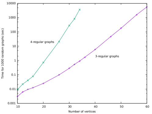
Figure 1: The running times for computing the genus of 1000 random cubic, resp. quartic graphs. Note that the time scale is logarithmic.

If we fix the number of vertices, but vary the number of edges, we get – as expected – again an exponential growth, as shown in Figure 2.

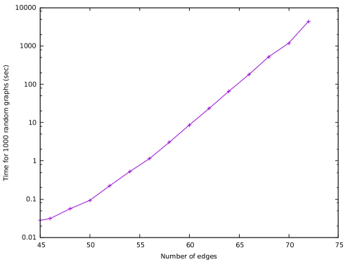
Figure 2: The running times for computing the genus of 1000 random graphs with 32 vertices and a given number of edges. Note that the time scale is logarithmic.

Together with the number of vertices and edges, also the average genus increases, so it is also interesting to know how the running times develop, when it is only tested whether the graphs can be embedded in a surface of given genus – similar to planarity testing. In Figure 3 the running times for testing whether 1000 random cubic resp. quartic graphs can be embedded in a surface of genus at most 3 are given. In fact for practically all of the larger graphs tested, the answer was no. Nevertheless it is astonishing that from a certain point on the time necessary to test a graph decreases again.

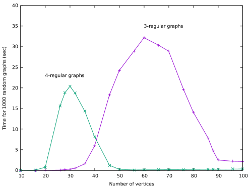
Figure 3: The running times for testing 1000 random cubic, resp. quartic graphs for having genus at most 3.

If one wanted to apply the algorithm to perform very well when testing only planarity, one could apply the reasoning of Demoucron, Malgrange and Pertuiset [8] as soon as a spanning tree and the first cycle is formed. Of course that would not be useful, as specialized and very efficient algorithms for planarity testing exist. Although no special adaptation for the planar case is implemented and this is not the task the algorithm was developed for, a comparison with specialized programs for planarity testing might be interesting. In [3] a practical linear time algorithm for planarity testing is presented. In the program planarg [10] an implementation of this algorithm by Paulette Lieby is available.

Testing 100,000 random cubic graphs on 50 vertices with planarg and multi_genus with 0 as an upper bound for the genus, the times are 2.29 (planarg) resp. 5.5 (multi_genus) seconds. Testing 100,000 random cubic graphs on 100 vertices, planarg is more than 4 times faster than multi_genus (5.0 seconds to 22.1 seconds). All these graphs were non-planar. Filtering the 11,529 rome graphs for non-planar ones took 0.36 seconds with planarg and 0.29 seconds with multi_genus. In this case about 28% of the graphs were planar. In order to test how fast embeddings are found if they exist, once sparse planar graphs – that is cubic graphs – were tested and once dense graphs – that is triangulations. For these tests, for multi_genus no lower bound for the genus was computed. We used the 285,914 fullerenes on 100 vertices and their duals (triangulations on 52 vertices) randomly relabeled in order to avoid an impact of the embedding produced by the generation program. For the fullerenes, planarg needed 19.5 seconds (compared to 19.1 seconds for multi_genus) and for the triangulations planarg needed 11.85 seconds (compared to 11.1 seconds for multi_genus).

Testing

In order to test the implementation, independent programs were used and the results were compared to the results of multi_genus. For all cases tested the results agreed.

In order to test the option to compute the genus, the genus of each (connected) graph in the following set was computed by multi_genus and MinGenusEmbedder and the result was compared. The sets of graphs are: all graphs on up to 11 vertices, all 3-regular graphs on up to 24 vertices, all 4-regular graphs on up to 16 vertices, all 5-regular graphs on up to 14 vertices, all 3-regular graphs on up to 26 vertices with girth at least 5, all 3-regular graphs on up to 28 vertices with girth at least 6, all 3-regular graphs on up to 34 vertices with girth at least 7, all 3-regular graphs on up to 44 vertices with girth 8, all (3,9)-cages – that is all 3-regular graphs on 58 vertices with girth 9, all 4-regular graphs on up to 24 vertices with girth 5, and finally all graphs with valence vector $(2,2,3,3,3)$.

In order to test the option that makes multi_genus generate all embeddings of a certain genus, a simple independent program was implemented that generated all combinations of all vertex orders around the vertices. Filtering the embeddings generated this way for those with a given genus we had a very slow but independent test. Then for each graph in one of the following sets, the range of possible genera was computed by the Euler formula and for each graph and each possible genus the embeddings of this genus were independently generated and the number of embeddings as well as the number of non-isomorphic embeddings (computed by an isomorphism checking program using lists) were compared. Due to the enormous number of embeddings already for small graphs, not too many graphs and no large graphs could be tested. The sets of graphs are: all 3-regular graphs on up to 18 vertices, all graphs on 7 vertices with 6 to 17 edges, all graphs on 8 vertices with 14 and with 15 edges, all graphs with valence vector $(1,1,1,5)$, and finally all graphs with valence vector $(0,2,3,2,3)$ and girth at least 4.

Results obtained or confirmed by multi_genus

Times given for multi_genus in this section are again on an Intel Core i7-9700 CPU @ 3.00GHz running on one core at 4.4-4.7 Ghz.

In [12] Plummer and Zha prove a theorem describing the cases when $K_{c+1}$ is the unique c-connected graph with smallest genus – except for the two cases $c=9$ and $c=13$ which are not decided and posed as an open question. This question is answered in [2] showing that in these cases the complete graphs are not unique, but that in these cases the graphs $M_{c+2}$ on $c+2$ vertices, obtained by deleting a maximum matching from $K_{c+2}$, have the same genus as $K_{c+1}$. The embeddings given in that article were computed by multi_genus. Computing the genus $g(M_{11})=4$ takes $0.005$ seconds and computing the genus $g(M_{15})=10$ takes $7$ hours and $6$ minutes.

In [6] Conder and Grande determine all circulant graphs of genus 1 and 2. A large part of the proof discusses 12 specific circulant graphs and in order to prove that 11 of these graphs have genus larger than 2, next to several pages of theoretical argumentation also more than 80 CPU hours were needed. The program described in [1] confirms these results in 180 hours of CPU time (without additional theoretical arguments), and ILP${}^{\mbox{\tiny D}}_{\mbox{\tiny Real}}$ computes the genera in a matter of seconds (the exact value isn’t given). Multi_genus confirms the results of the paper in less than $0.03$ seconds. Computing the exact genera (once genus 2, 7 times genus 3, 3 times genus 4, and once genus 5) and minimum genus embeddings takes $6.4$ seconds.

In [9] the genus of the Gray graph is theoretically determined by a nontrivial construction. ILP${}^{\mbox{\tiny D}}_{\mbox{\tiny Real}}$ confirms this result within $42$ hours. Multi_genus confirms this in $28.3$ seconds. In order to determine all $258,696$ (labeled) minimum genus embeddings ($219$ non-isomorphic), multi_genus needed a bit less than $10$ minutes. Isomorphism rejection is done by an independent program simply storing canonical embeddings in lists.

In [7] the genus (and also non-orientable genus) of several graphs was determined. They describe four specialized approaches they apply to some special graphs that have in general a large symmetry group. One of them – they call it the subgroup orbit method – is especially suited for as they write graphs on surfaces with a certain degree of symmetry and works well for graphs that allow an embedding with a face-transitive automorphism group. So the approach is far from general and the program is also not available for everybody. Our general approach cannot reproduce their results for the Hoffman-Singleton graph, the Ljubljana graph or the Iofinova-Ivanov graph – at least not without an excessive amount of time and/or special adaptations. Some of the other examples they give can also be solved and sometimes extended by our general approach without any manual interference – just by piping the graph into multi_genus. In [7] in general no precise running times are given. The instances for which the results could be confirmed and sometimes extended are:

The graph $C_{3}\square C_{3}\square C_{3}$: In [7] it says that with a natural vertex labeling the subgroup orbit method takes only a couple of minutes to find a genus 7 embedding. The method described here takes – depending on the labeling – from $0.19$ seconds to $281$ seconds to find an embedding. Of course there may also be labelings that take even less or even more time. In total there are 188,211,024 minimum genus embeddings, 145,468 of them pairwise non-isomorphic, but computing these took almost 3 weeks of CPU time (on another, much older, machine used for the large memory available for isomorphism rejection).

Not only constructing a genus 7 embedding, but also proving its minimality by excluding the existence of an embedding of smaller genus takes between $1.5$ and $4$ hours depending on the labeling (both with BFS numbering first).

The Tutte graph (or $(3,8)$-cage): In [7] no running times are given, but they construct a genus $4$ embedding with cyclic automorphism group of order $3$. The present approach takes $0.005$ seconds to determine the genus as $4$ and $0.13$ seconds to construct all $13,440$ embeddings. Among these embeddings there are $15$ non-isomorphic embeddings – $4$ with group size $1$, $10$ with group size $2$ ($2$ of them allowing a reflection) and one with group size $3$.

The Gray graph: The running times for the Gray graph were already given. In [7] it is reported that there are minimum genus embeddings with an automorphism group of order 6. Checking all possible embeddings, the result is that there are $186$ non-isomorphic embeddings with trivial symmetry, $23$ with group size $2$, $4$ with group size $3$, $4$ with group size $6$, and $2$ with group size $18$.

The Folkman graph: For the Folkman graph, in [7] minimum genus embeddings with group size $8$ are constructed. The method described here takes less than $0.001$ seconds to determine the genus as $3$ and $0,037$ seconds to construct all $7,680$ minimum genus embeddings. Among these embeddings there are $7$ pairwise non-isomorphic, $2$ with group size $2$, $3$ with group size $4$, and $2$ with group size $8$. All groups contain a reflection.

The Doyle-Holt graph: For the Doyle-Holt graph [7] describes a genus $5$ embedding with an automorohism group of size $2$. The present approach needs $0.23$ seconds to determine the genus of the graph and $7.3$ seconds to determine all $1,107$ minimum genus embeddings. There are $24$ pairwise non-isomorphic embeddings – $17$ with trivial group and $7$ with group size 2.

The dual Menger graph of the Gray configuration: For this 6-regular graph on 27 vertices, the present approach needs $20$ seconds to determine the genus as $6$. In a bit more than $26$ minutes it constructed all $216$ minimum genus embeddings – which turned out to be isomorphic. So the minimum genus embedding of the dual Menger graph of the Gray configuration is unique. It has automorphism group size $6$.

References

- [1] S. Beyer, M. Chimani, I. Hedtke, and M. Kotrbčík. A practical method for the minimum genus of a graph: Models and experiments. In SEA 2016, LNCS 9685, pages 75–88. 2016.
- [2] D. Bokal, G. Brinkmann, and C. T. Zamfirescu. The connectivity of the dual. submitted, arXiv:1812.08510.
- [3] J. Boyer and W. Myrvold. Stop minding your p’s and q’s: A simplified O(n) planar embedding algorithm. Tenth Annual ACM-SIAM Symposium on Discrete Algorithms (SODA), pages 140–146, 1999.
- [4] G. Brinkmann, J. Goedgebeur, H. Mélot, and K. Coolsaet. House of graphs: a database of interesting graphs. Discrete Applied Mathematics, 161:311–314, 2013. http://hog.grinvin.org.
- [5] M. Chimani and T. Wiedera. Stronger ilps for the graph genus problem. In 27th Annual European Symposium on Algorithms, pages 30:1–30:15, 2019. (ESA 2019).
- [6] M. Conder and R. Grande. On embeddings of circulant graphs. Electr. J. Comb., 22(2), 2015. P2.28.
- [7] M. Conder and K. Stokes. New methods for finding minimum genus embeddings of graphs on orientable and non-orientable surfaces. Ars Mathematica Contemporanea, 17:1–35, 2019.
- [8] G. Demoucron, Y. Malgrange, and R. Pertuiset. Graphes Planaires: Reconnaissance et Construction de Representations Planaires Topologiques. Rev. Franc. Rech. Oper., 8:33 – 34, 1964.
- [9] D. Marusic, T. Pisanski, and S. Wilson. The genus of the gray graph is 7. Eur. J. Comb., 26(3-4):377–385, 2005.
-
[10]
B.D. McKay.
http://cs.anu.edu.au/~bdm/nauty/. - [11] B. Mohar. A linear time algorithm for embedding graphs in an arbitrary surface. SIAM J. Discrete Math, 12:6–26, 1999.
- [12] M. D. Plummer and X. Zha. On the connectivity of graphs embedded in surfaces. J. Combin. Theory, Ser. B, 72:208–228, 1998.
- [13] C. Thomassen. The graph genus problem is np-complete. J. Algorithms, 10:568–576, 1989.