Science with the TianQin observatory: Preliminary result on extreme-mass-ratio inspirals

Abstract

Systems consisting of a massive black hole and a stellar-origin compact object (CO), known as extreme-mass-ratio inspirals (EMRIs), are of great significance for space-based gravitational-wave detectors, as they will allow for testing gravitational theories in the strong field regime, and for checking the validity of the black hole no-hair theorem. In this work, we present a calculation of the EMRI rate and parameter estimation capabilities of the TianQin observatory, for various astrophysical models for these sources. We find that TianQin can observe EMRIs involving COs with mass of 10$M_{\odot}$ up to redshift $\sim 2$. We also find that detections could reach tens or hundreds per year in the most optimistic astrophysical scenarios. Intrinsic parameters are expected to be recovered to within fractional errors of $\sim 10^{-6}$, while typical errors on the luminosity distance and sky localization are 10% and 10 deg², respectively. TianQin observation of EMRIs can also constrain possible deviations from the Kerr quadrupole moment to within fractional errors $\lesssim 10^{-4}$. We also find that a network of multiple detectors would allow for improvements in both detection rates (by a factor $\sim 1.5$ -$3$) and in parameter estimation precision (20-fold improvement for the sky localization and fivefold improvement for the other parameters).

I Introduction

Gravitational-wave (GW) observations provide information on the minute vibrations of the spacetime, and promise to revolutionize astronomy and astrophysics by opening a new window on the Universe. To date, the ground-based GW observatories, LIGO and Virgo, have detected several GW events Abbott et al. (2019, 2020a, 2020b, 2020c). Limited by seismic noise and their relatively short arm lengths, however, ground-based detectors are sensitive only to high-frequency GWs (above a few hertz) generated by low-mass sources [e.g., mergers of stellar-origin compact objects(COs)]. In order to detect heavier sources, such as ones involving massive black hole (MBH), or even the low-frequency (subhertz) inspiral phase of stellar-origin compact binaries Sesana (2016), a significant increase in the size of GW detectors is necessary, which can be achieved only in space. LISA, for example, will present arm lengths of about 2.5 million km and will be sensitive to GWs in the frequency band $10^{-5}$ -$0.1$ Hz Amaro-Seoane et al. (2017); Baker et al. (2019).

TianQin is a proposed space-based, geocentric GW observatory with arm lengths of about $1.7\times 10^{5}$ km, aiming to detect GW signals in the frequency band $10^{-4}$ -$1$ Hz Luo et al. (2016); Hu et al. (2019). In the past few years, a systematic effort has been undertaken to study the science prospects of TianQin Hu et al. (2017). On the astrophysics side, this included the study of the detection prospects for Galactic ultracompact binaries Huang et al. (2020), coalescing MBHs Wang et al. (2019); Hu et al. (2018), the low-frequency inspiral of stellar-mass black holes Liu et al. (2020), and stochastic GW backgrounds Liang et al. (2020). On the fundamental physics side, TianQin’s ability to test the black hole no-hair theorem with the ringdown of MBHs resulting from a merger has been analyzed, both in a theory-agnostic framework Shi et al. (2019) and within specific gravitational theories extending general relativity Bao et al. (2019), and more work is in preparation in this direction.

In this paper, we focus on extreme-mass-ratio insprials (EMRIs), i.e., binaries consisting of a stellar-origin CO (a stellar mass black hole or a neutron star) orbiting around a MBH in a long inspiral Amaro-Seoane et al. (2007); Berry et al. (2019). These sources are expected to be relatively numerous in the millihertz GW sky probed by LISA and TianQin. Indeed, strong observational evidence suggests the presence of MBHs at the center of most local galaxies Kormendy and Richstone (1995a); Magorrian et al. (1998); Gebhardt et al. (2003); Ferrarese and Ford (2005), typically surrounded by stellar clusters or cusp sAlexander (2005); Schödel et al. (2014) of a few parsec scale. Relaxation processes in such a high-density environment occasionally force stars and compact objects onto extremely eccentric, low angular momentum orbits, resulting in a close encounter with the central MBH. While main sequence stars are torn apart and tidally disrupted, potentially resulting in luminous flares and prompting gas accretion onto the central MBH Hills (1975); Murphy et al. (1991); Freitag and Benz (2002); Gezari et al. (2003), COs typically survive intact until merger Merritt (2015); Bar-Or and Alexander (2016); Amaro-Seoane (2019). Depending on their orbital angular momentum, COs can directly plunge into the MBH or be captured in eccentric bound orbits, whose secular evolution decouples from the cluster’s dynamics and is dominated by GW emission Amaro-Seoane et al. (2007). These latter systems are usually referred to as EMRIs.

Detecting GWs from EMRIs will be very significant for our understanding of the astrophysics of these sources Amaro-Seoane et al. (2007). For instance, it will allow for gaining information on the mass distribution of MBHs Gair et al. (2010) and their host stellar environments Amaro-Seoane et al. (2007). It may also provide information on the expansion of the Universe MacLeod and Hogan (2008), as well as allow for mapping the spacetime geometry of the MBH in great detail so that a stringent test of general relativity is possible Gair et al. (2013), through measuring the bumpy nature of black holes Piovano et al. (2020), investigating the non-Kerr nature of central objects Glampedakis and Babak (2006), constraining modified gravity theories Niu et al. (2019), and testing the no-hair theorem Ryan (1995, 1997a, 1997b); Barack and Cutler (2007); Chua et al. (2018). Futhermore, it can also reveal the possible presence of matter surrounding MBHs through their effects on waveforms Barausse et al. (2007); Barausse and Rezzolla (2008); Gair et al. (2011); Yunes et al. (2011); Barausse et al. (2014, 2015); Derdzinski et al. (2020).

To estimate the detection rate for EMRIs with a specific detector, one would need the corresponding astrophysical models as input, including the description of the population properties as well as the event rates Mapelli et al. (2012); Berry et al. (2016); Bortolas and Mapelli (2019). In this paper, we use previously published astrophysical models Babak et al. (2017) for the formation and evolution of EMRIs across cosmic time to assess TianQin’s capability to detect these sources and estimate their parameters. In more detail, by adopting, as was done in Ref. Babak et al. (2017) for LISA, analytic kludge waveforms and using a simple Fisher information matrix (FIM) method to analyze the parameter estimation prospects, we find that EMRIs can be observed up to redshift $\sim 2$, assuming a 10 $M_{\odot}$ CO, with rates vary from $10$ to 100 yr^-1. Intrinsic parameters are projected to be estimated to within fractional errors of $\sim 10^{-6}$, while typical errors on the luminosity distance and sky localization are 10% and 10 deg², respectively. We also estimate the potential scientific gain of operating TianQin within a network of detectors, e.g., together with LISA and/or a twin TianQin detector (TQ II). We find that a twin TianQin detector would increase detection rates by a factor of $\sim 1.5$ -$3$.

The paper is organized as following. In Sec. II, we describe our model for the EMRI astrophysical population, the gravitational waveforms, the response of TianQin to extreme mass ratio inspiral (EMRI) signals and the TianQin noise model used in this study. In Sec. III, we describe the method for calculating the signal-to-noise ratio (SNR) and the precision of the parameter estimation. The main results of our study are presented in Sec. IV. In Sec. V, we present our conclusions.

II The model

II.1 EMRI rate

Extensive evidence exists for the ubiquitous presence of MBHs at the center of virtually every galaxy at low redshifts Lynden-Bell and Rees (1971); Soltan (1982); Kormendy and Richstone (1995b); Gultekin et al. (2009), including our own Milky Way Schodel et al. (2002); Reid et al. (1999, 2003); Abuter et al. (2018) and, as recently confirmed by the Event Horizon Telescope, M87 Akiyama et al. (2019). Moreover, nuclear stellar clusters with sizes of a few parsecs(pc) and masses up to $10^{7}$ -${10^{8}}M_{\odot}$ are also known to coexist with MBHs in the local Universe (except at the high-mass end of the MBH mass function) Schödel et al. (2014). The high densities of these clusters make them the perfect cradles for the formation of EMRIs, as two-body relaxation will make the system tend toward energy equipartion and, thus, mass segregation, with the heavier objects (i.e., stellar-mass black holes) sinking deeper in the MBH gravitational potential well. This process can eventually lead to COs plunging or inspiraling into the MBH, depending on their angular momenta.

The rate of EMRIs and their properties depend on a variety of (astro)physical processes, which determine the evolution of the population of MBHs along cosmic history and the accumulation of COs in their vicinity. In this paper, we make use of the EMRI population models developed by Babak et al. Babak et al. (2017). For the convenience of the readers, we summarize the main features of the model here but refer to Ref. Babak et al. (2017) for more details. The intrinsic EMRI rate is given by the following function:

$${\cal R}(M,z,a)=\frac{d^{3}N}{dMdzda}\times p_{0}(M,z)\times\kappa\Gamma{R_{0}(M)}\,,$$ (1)

where $M,z,$ and $a$ are the mass, redshift, and spin of the MBH, respectively. Terms on the right-hand side of this equation are explained below.

• $d^{3}N/(dMdzda)$ is the redshift-dependent MBH mass function. Two scenarios have been adopted that bracket the uncertainties in the low-mass end of the MBH mass function at $z=0$. One scenario is based on the semianalytic model (SAM) developed by Barausse and collaborators in a series of papers Barausse (2012); Sesana et al. (2014); Antonini et al. (2015). The SAM follows the formation and evolution of MBH masses and spins along cosmic history, and produces a mass function $dN/d{\rm log}M\propto M^{-0.3}$ in the range $10^{5}{\rm M}_{\odot}<M<10^{7}{\rm M}_{\odot}$, consistent with the upper bound of current observations (see Fig. 1 in Ref. Babak et al. (2017)). A second scenario employs an empirical mass function where $dN/d{\rm log}M\propto M^{0.3}$ in the same mass range $10^{5}{\rm M}_{\odot}<M<10^{7}{\rm M}_{\odot}$ Gair et al. (2010), consistent with the lower bound of current observations.

• $p_{0}(M,z)$ describes the probability that a MBH with mass $M$ and redshift $z$ is surrounded by a cusp of stars and COs, thus potentially giving rise to an active EMRI source. When two galaxies merge, the cusps of stars and COs around the central MBHs of the parent galaxies are eroded by the action of the inspiraling MBH binary. The cusp in the merger remnant is, therefore, destroyed, and is rebuilt only after a fraction of the relaxation time Amaro-Seoane and Preto (2011). The SAM model allows one to follow the galaxy and MBH merger rate and to estimate the time needed to rebuild the cusp, from which the probability function for each MBH to be a potential EMRI source is constructed.

• ${R_{0}(M)}$ is the rate at which a galaxy hosting a MBH with mass $M$ surrounded by a stellar (and CO) cusp actually generates an EMRI. Note that this probability depends on the density profile of the CO population, which might depend on the redshift and other parameters unrelated to the MBH mass. For simplicity, however, any such possible dependence is dropped, and ${R_{0}(M)}$ is assumed to be a function of the MBH mass only, following Ref. Amaro-Seoane and Preto (2011).

• Finally, $\kappa$ and $\Gamma$ are two “ad hoc” correction factors to ${R_{0}(M)}$ that ensure that the overall EMRI rate is consistent with the observed MBH mass function, i.e., that the MBHs do not “overgrow‘” their present masses by capturing too many EMRIs and plunges.

Besides the choice of two different MBH mass functions, Eq. (1) – and the observed EMRI rate –also depends on a number of additional astrophysical factors, including:

• The relative occurrence rate of plunges versus EMRIs, which enters in the $\Gamma$ factor.–The plunge cross section of the MBH itself ($4GM/c^{2}$ for a nonrotating MBH) is not negligible compared to the EMRI capture cross section, which is generally $<10GM/c^{2}$. Recent simulations have actually found that plunges are typically more frequent than EMRIs Merritt (2015), and this has an impact on the intrinsic EMRI rate for a given MBH.

• The choice of parameters of the MBH-galaxy scaling relations, which is important to compute the $p_{0}(M,z)$ function.–In fact, the time needed to rebuild the cusp depends on the properties of the galactic nucleus, whose mass can be computed from the MBH mass via the MBH-galaxy scaling relations.

• The MBH spin distribution, which has an impact both on the EMRI capture rate and the EMRI waveforms, and, hence, on their detectability with GWs (as shown in the following section).

• The mass of the CO, which affects the rate normalization and which enters the EMRI waveforms.–Most models in Ref. Babak et al. (2017) assume COs with $10{\rm M}_{\odot}$, but some consider COs with $30{\rm M}_{\odot}$.

The above ingredients have been suitably combined in Ref. Babak et al. (2017) to build a suite of 12 models encompassing three orders of magnitude in the expected cosmic EMRI rate, from 10 to about $2\times 10^{4}$ yr^-1. These are also the models that we employ in this investigation. We label the models as M-$i$ with $i=1,\dots,12$, following the original nomenclature. Detailed prescriptions for each model can be found in Table I of Ref. Babak et al. (2017).

II.2 Waveform

The calculation of the waveforms for EMRIs is a challenging task. Although much progress has been attained with the goal of producing accurate and efficient EMRI waveforms including the effect of the self-force Drasco and Hughes (2006); Warburton et al. (2012); van de Meent (2016); Warburton (2015); Huerta and Gair (2009); Van De Meent and Warburton (2018); Pound et al. (2020), the problem has not been fully solved yet. Here, we adopt simple waveforms suitable for predicting the detection and parameter estimation capabilities of TianQin, but one should keep in mind that full waveforms including the effect of the self-force will be needed to analyze the real data.

In more detail, in this paper we follow Ref. Babak et al. (2017) and utilize a class of simplified and approximate but computationally inexpensive EMRI waveforms, the analytic kludge (AK) model from Ref. Barack and Cutler (2004). There are other kludge waveforms available for EMRI events, like the numerical kludge (NK) Glampedakis et al. (2002); Gair and Glampedakis (2006); Babak et al. (2007) or the augmented analytic kludge (AAK) Chua and Gair (2015); Chua (2016); Chua et al. (2017), with NK being significantly slower than AK and AAK being comparable to AK in terms of computing time. Both the NK and the AAK waveform are physically more self-consistent compared with the AK waveform, but neither is fully consistent, and for the sake of fair comparison, we stick with the AK waveform for the following computations.

The AK waveform is calculated simply from the quadrupole formula, while the orbital evolution of the CO includes post-Newtonian (PN) corrections accounting for pericenter precession, Lense-Thirring precession, and (leading-order) radiation reaction.

The waveform far away from the source is given in the transverse traceless gauge by

$$h_{ij}=\frac{2}{D}(P_{ik}P_{jl}-\frac{1}{2}P_{ij}P_{kl})\ddot{I}^{kl}\,,$$ (2)

where $D$ is the source distance, $P_{ij}\equiv\eta_{ij}-\hat{n}_{i}\hat{n}_{j}$ is the projection operator on the space orthogonal to the unit vector of the source position $\hat{n}$, and $\ddot{I}^{ij}$ is the second time derivative of the quadrupole. For an EMRI system with CO mass $m$, central MBH mass $M$, and mass ratio $m/M\ll 1$, we have $I^{ij}(t)=mr^{i}(t)r^{j}(t)$, where $\vec{r}$ is the displacement vector of the CO from the MBH.

The orbit evolution of the CO is described by the first-order derivative of the following five quantities:

• $\Phi$, the mean anomaly of the CO’s orbit;

• $\nu$, the orbital frequency;

• $e$, the orbital eccentricity;

• $\alpha$, the azimuthal angle of the CO orbital angular momentum $\vec{L}$ with respect to the MBH’s spin angular momentum $\vec{S}$; and

• $\tilde{\gamma}$, the direction of the pericenter relative to $\vec{L}\times\vec{S}$.

The evolution equations for $\Phi$, $\nu$, and $e$ include terms up to 3.5PN order. The evolution of $\alpha$ caused by Lense-Thirring precession and that of $\tilde{\gamma}$ caused by pericenter precession are instead followed up to 2PN order. The equations depend on the two masses $m$ and $M$, the dimensionless spin $a=S/M^{2}$, and the angle $\lambda$ between $\vec{L}$ and $\vec{S}$. For a distant source, the masses should be replaced by “redshifted” mass $m_{z}=m(1+z)$ and $M_{z}=M(1+z)$. To test the no-hair theorem, one can also introduce an arbitrary quadrupole moment $Q$ for the central MBH in the evolution equations. The explicit form of the evolution equations is given in Eqs. (27-31) of Ref. Barack and Cutler (2004) (without $Q$) and in Eqs. (4-8) of Ref. Barack and Cutler (2007) (with an arbitrary $Q$). Obviously, the orbital evolution depends on the initial conditions at some initial time $t_{0}$. To obtain the waveform, we also need five other extrinsic parameters, namely, the source’s sky position ($\theta_{S}$, $\phi_{S}$), the luminosity distance $D$, and direction of the MBH’s spin $\vec{S}$ relative to the line of sight ($\theta_{K}$ and $\phi_{K}$). In summary, there are 14 parameters, $(t_{0},m,M,a,e_{0},\tilde{\gamma}_{0},\Phi_{0},\theta_{S},\phi_{S},\lambda,\alpha_{0},\theta_{K},\phi_{K},D_{L})$, with the additional parameter $Q$ introduced when testing the no-hair theorem.

In Ref. Barack and Cutler (2004), the waveform was conventionally cut off at the last stable orbit (LSO) $r_{\rm LSO}$ of the Schwarzschild spacetime. We refer to this as the AK Schwarzschild (AKS) case. However, since the exact value of the cutoff frequency can have a significant impact on the parameter estimation, we also consider, as in Ref. Babak et al. (2017), an AK Kerr (AKK) waveform model where we cut the waveform off at the Kerr LSO. As argued in Ref. Babak et al. (2017), more realistic EMRI waveforms including dissipative self-force effects should yield results between the (more conservative) AKS results and the (more optimistic) AKK ones.

II.3 Detector response

TianQin will consist of three satellites orbiting the Earth, forming a regular triangular constellation, with each side measuring about $L=1.7\times 10^{8}$ m. The detector orientation, i.e., the direction normal to the plane of the constellation, will point to a reference source, the white dwarf binary system RX J0806.3+1527 (J0806 for short). The nominal operation time of TianQin will be 5 yr, which is assumed throughout this paper. There is expected to be only a very small drift of the detector orientation over a 5-yr period Ye et al. (2019), and, since that should have negligible effect on the present study, we will not consider it. The location of J0806 is close to the ecliptic plane, so the constellation plane of TianQin will be nearly perpendicular to the ecliptic plane. The TianQin satellites will have nearly identical orbits and nearly identical periods, which will be about $T=3.6$ days Luo et al. (2016); Hu et al. (2017, 2019).

In the Solar Ecliptic Coordinate System where the x axis points towards the direction of the vernal equinox and the z axis is normal to and northward from the ecliptic plane, the location of the satellites at a given time can be formulated as Hu et al. (2018)

$$x(t) = R\cos\alpha_{e}+\frac{1}{2}R\cdot e_{e}\cdot\cos(2\alpha_{e}-3)$$

$$+\frac{1}{\sqrt{3}}L\cdot(\cos\theta\cos\phi\cos\gamma_{e}-\sin{\phi}\sin{\gamma_{e}})\,,$$

$$y(t) = R\sin\alpha_{e}+\frac{1}{2}R\cdot e_{e}\cdot\sin(2\alpha_{e})$$

$$+\frac{1}{\sqrt{3}}L\cdot(\cos\theta\sin\phi\cos\gamma_{e}+\cos{\phi}\sin{\gamma_{e}})\,,$$

$$z(t) = -\frac{1}{\sqrt{3}}L\cdot\sin\theta\cos\gamma_{e}\,,$$ (3)

where $R=1$AU is the semimajor axis, $e_{e}=0.0167$ is the eccentricity, and $\alpha_{e}=2\pi{f_{e}}t+\Phi_{e}$ is the phase, with $f_{e}=1/$yr and $\Phi_{e}$ being, respectively, the frequency and initial phase of the orbit of Earth. The angular parameters ($\theta$, $\phi$) specify the space direction to J0806, and $\gamma_{e}=2\pi{t}/T+2\pi{n}/3+\delta$ $(n=1,2,3)$ are the phases of the satellites in their geocentric orbits, where $\delta$ is some reference phase that can be set to zero.

The effect of a propagating GW ${h}(\xi)$ on the optical path length $L_{ij}$ starting from the satellite $i$ at time $t-L_{ij}$ and arriving at the satellite $j$ at time $t$ can be expressed as Cornish and Larson (2001); Rubbo et al. (2004)

$$\delta{L}_{ij}(t)=\frac{1}{2}\frac{\hat{r}_{ij}(t)\otimes\hat{r}_{ij}(t)}{1-\hat{k}\cdot\hat{r}_{ij}(t)}:\int^{\xi_{j}}_{\xi_{i}}{h}(\xi)d\xi\,,$$ (4)

where $\xi_{i}$ is the phase and $\hat{r}_{ij}(t)$ is the unit vector from the satellite $i$ to the satellite $j$ at time $t$. Two independent Michelson interferometer signals can be constructed Cutler (1998):

$$h_{1}(t) = [\delta{L_{12}}(t)-\delta{L_{13}}(t)]/L\,,$$

$$h_{2}(t) = \frac{1}{\sqrt{3}}[\delta{L_{12}}(t)+\delta{L_{13}}(t)-\delta{L_{23}}(t)]/L\,.$$ (5)

Note that the orbital motion of the TianQin satellites also contributes a phase modulation (due to the Doppler shift) to the observed signal:

$$\Phi^{D}(t)=2\pi\nu(t)R\sin\theta_{S}\cos[\phi(t)-\phi_{S}]\,,$$ (6)

where $2\nu$ is the frequency of the GW signal, ($\theta_{S}$, $\phi_{S}$) are the angular coordinates of the source, and $\phi(t)=\alpha_{e}$ is the orbit phase.

II.4 Detector noise

The noise model of TianQin is encoded in the following sensitivity curve Huang et al. (2020); Wang et al. (2019); Shi et al. (2019); Finn (1992):

$$S_{n}(f) = \frac{1}{L^{2}}\left[\frac{4S_{a}}{(2\pi f)^{4}}\left(1+\frac{10^{-4}{\mathrm{H}z}}{f}\right)+S_{x}\right]$$ (7)

$$\times\left[1+0.6\left(\frac{f}{f_{*}}\right)^{2}\right]\,,$$

where $S_{a}^{1/2}=1\times 10^{-15}$m s${}^{-2}/$Hz^1/2 characterizes the residual acceleration on a test mass playing the role of an inertial reference, $S_{x}^{1/2}=1\times 10^{-12}$m/Hz^1/2 characterizes the one-way noise of the displacement measurement with intersatellite laser interferometry, and $f_{*}=1/(2\pi L)$ is the transfer frequency Luo et al. (2016). An illustration of the sensitivity curve of TianQin is given in Fig. 1. For comparison, we also plot the LISA sensitivity curve in Fig. 1 based on Ref. Babak et al. (2017).

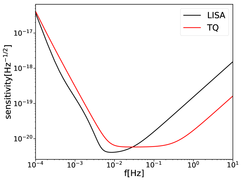
Figure 1: The sensitivity curve for TianQin and LISA.

At the low-frequency end of the TianQin observation range, there exist numerous compact binaries in the Galaxy, whose GW signals overlap to give rise to a stochastic unresolved signal, sometimes referred to as the foreground. Preliminary analyses suggest that such a foreground will be consistently below the sensitivity curve for resolved sources, given that the operation time of TianQin is limited to 5 yr Liang et al. (2020). We therefore do not consider the effect of Galactic compact binaries throughout this work.

III Method

III.1 Signal-to-noise ratio

In order to study the prospects of detecting EMRIs with TianQin, one can calculate the SNR. Previous studies have shown that EMRIs with SNRs as low as 15 can be detected by LISA under favorable circumstances Babak et al. (2010). In this paper, we adopt the more conservative SNR threshold of 20 for detection, following Ref. Babak et al. (2017).

Using the noise-weighted inner product between two signals $s_{1}(t)$ and $s_{2}(t)$,

$$(s_{1}|s_{2})=2\int_{0}^{\infty}\frac{\tilde{s}_{1}(f)\tilde{s}_{2}^{\ast}(f)+\tilde{s}_{1}^{\ast}(f)\tilde{s}_{2}(f)}{S_{n}(f)}df\,,$$ (8)

where $\tilde{s}_{i}(f)$, $i=1,2,$ are the Fourier transforms of $s_{i}(t)$, the SNR can be defined as

$$\rho=(h|h)^{1/2}=2\Big{[}\int_{0}^{\infty}\frac{\tilde{h}(f)\tilde{h}^{\ast}(f)}{S_{n}(f)}df\Big{]}^{1/2}\,,$$ (9)

where $h(t)$ is the GW-induced signal in the detector. The Fourier transform $\tilde{h}(f)$ is obtained from $h(t)$ by applying a discrete Fourier transform:

$$\tilde{h}\left(\frac{k}{N\Delta t}\right)=\Delta{t}\sum^{N}_{n=1}h(n\Delta t)e^{-i2\pi{k}n/N},$$ (10)

where $\Delta{t}$ is the sampling interval.

The basic TianQin data stream consists of data segments each lasting for 3 months for protection from heat instability, and the total accrued SNR is obtained as the root sum square of the individual SNR from each data segment. The same root-sum-square rule is also used when combining the contributions from different interferometer signals (when we consider TianQin operating within a detector network).

III.2 Fisher information matrix

The existence of noise leads to uncertainties in the inference on source parameters. To quantify these uncertainties, we use the FIM method to obtain the lowest-order expansion of the posteriors (valid in the high SNR limit), which can be more accurately estimated through a full Bayesian parameter estimation analysis. Indeed, we note that the FIM method can be used as a fast assessment of the expected parameter estimation capabilities of an experiment, but the obtained $\Sigma$ represents only the Cramer-Rao bound of the covariance matrix. More advanced techniques are required to obtain more realistic results Vallisneri (2008); Rodriguez et al. (2013).

The FIM is defined as

$$\Gamma_{ij}=\Big{(}\frac{\partial\tilde{h}(f)}{\partial{\theta^{i}}}\Big{|}\frac{\partial\tilde{h}(f)}{\partial{\theta^{j}}}\Big{)}\,,$$ (11)

where $\theta^{i}$, $i=1,2,...,$ are the parameters appearing in the template $\tilde{h}(f)$. When multiple interferometers are present, the network’s FIM can be obtained as the sum of the individual FIM from each interferometer.

The EMRI waveform, even assuming the relatively simple AK model, is rather complicated, and it is difficult to obtain general analytical expressions for the partial derivatives $\partial{h(f)}/\partial{\theta^{i}}$. We therefore approximate derivatives with respect to the parameters by numerical finite differences. In the lowest-order expansion (i.e. in the high SNR limit), the variance-covariance matrix can be obtained as the inverse of the FIM:

$$\Sigma_{ij}\equiv\langle\delta\theta_{i}\delta\theta_{j}\rangle=(\Gamma^{-1})_{ij}.$$ (12)

From the variance-covariance matrix, the uncertainty $\sigma_{i}$ of the $i{\rm th}$ parameter $\theta_{i}$ can be obtained as

$$\sigma_{i}=\Sigma_{ii}^{1/2}\,.$$ (13)

We also note that it is often meaningful to discuss the sky localization in terms of the solid angle $\Delta\Omega$ corresponding to the error ellipse for which there is a probability $\exp(-1)$ for the source to be outside of it Babak et al. (2017), which can be expressed as a combination of the uncertainties on the ecliptic longitude angle $\phi_{S}$ and the ecliptic latitude angle $\theta_{S}$,

$$\Delta\Omega=2\pi\big{|}\sin\theta_{S}\big{|}\sqrt{\Sigma_{\theta_{S}}\Sigma_{\phi_{S}}-\Sigma_{\theta_{S}\phi_{S}}^{2}}\,.$$ (14)

IV Results

IV.1 Horizon distance

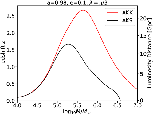
Figure 2: TianQin’s horizon distance for EMRI systems as a function of the MBH mass, assuming a MBH spin of 0.98, eccentricity of 0.1 and inclination angle of $\pi/3$. The black line adopts the AKS waveform, while the red curve adopts the AKK waveform.

As a first assessment of TianQin’s capability of detecting EMRIs, we compute the horizon distance, i.e., the farthest distance at which an EMRI source can be detected, or, equivalently, the farthest distance at which the SNR exceeds our detection threshold of 20, under the most favorable conditions possible Chen et al. (2017).

For the seven intrinsic parameters $m$, $M$, $S/M^{2}$, $e_{0}$, $\tilde{\gamma_{0}}$, $\phi_{0}$, and $\lambda$, we fix the mass of CO to $m=10M_{\odot}$ the orbital eccentricity to $e_{\rm lso}=0.1$, the MBH’s spin to $a=0.98$, and the inclination angle to $\lambda=\pi/3$, while the initial condition for $\tilde{\gamma_{0}}$ is set to 0, although that choice has a marginal effect on the SNR. One can see from Eq. (4) that TianQin has the strongest response to sources sitting on the line passing through the detector and J0806, so the source is placed in the direction of J0806. We also fix $\Phi_{0},\alpha_{0}$ to 0 and $\theta_{K},\phi_{K}$ to $\pi/4$,while the plunge time is taken to be 5 yr, which is the mission time of TianQin. These values of the parameters are all set at the moment when the CO reaches the Kerr LSO of the MBH.

The maximum redshift at which EMRIs can be detected by TianQin with a threshold SNR of 20 is illustrated in Fig. 2 as a function of the MBH mass. The red curve (corresponding to AKK waveforms) would allow for a larger detection range and features better sensitivity to systems with heavier MBHs than the black curve (which more conservatively uses AKS waveforms). This is mainly due to the fact that, by adopting a cutoff at later times (i.e., higher frequencies), the AKK waveforms include the larger GW amplitudes emitted when the CO is very close to the MBH. Thus, farther events are expected to be detectable under the fixed SNR threshold. The maximum horizon distance for AKK waveforms corresponds to $z\approx 2.6$, and to a MBH mass around $4\times 10^{5}M_{\odot}$. For the AKS waveform, on the other hand, the maximum horizon distance is smaller, with a corresponding redshift of about 1.6. The MBH mass for which the AKS horizon distance peaks is also smaller and around $2\times 10^{5}M_{\odot}$. This feature can also be explained in a simple manner: For the same EMRI system, AKK waveforms extend to higher frequencies, but that high-frequency component is most important for high-mass systems, whose low-frequency inspiral produces little SNR as it lies at lower frequencies than TianQin’s sensitivity sweet spot. Therefore, when using AKS waveforms (for which that high-frequency part is absent), the SNR of high-mass EMRIs is suppressed.

IV.2 Detection rate

Table 1: The expected detection rate of EMRIs with TianQin for different astrophysical models. The physical assumptions of the 12 models are described in Table I of Ref. Babak et al. (2017). The numbers are broken into different MBH mass ranges in the middle three columns, $M_{10}\equiv\log_{10}(M/M_{\odot})$, while the rightmost column summarizes the total detection rate. Numbers in brackets correspond to detection rates with AKS waveforms, while numbers outside brackets assume the AKK waveform.

Model	event rate (yr-1)	Detection rate of TianQin in mass range (yr-1)			Total (yr-1)
		$M_{10}<5$	$5<M_{10}<6$	$6<M_{10}$
M1	1600	1(1)	25(11)	8 (1)	34 (13)
M2	1400	0(0)	18(12)	2(0)	20 (12)
M3	2770	0(0)	83(28)	27 (2)	110(30)
M4	520	1 (0)	42(28)	7(3)	49(31)
M5	140	0(0)	4(2)	4(0)	8(2)
M6	2080	1(1)	40(22)	23(0)	64(23)
M7	15800	18(18)	187(121)	55(4)	260(143)
M8	180	0(0)	5(0)	1(0)	6(0)
M9	1530	2(1)	16(14)	2(1)	20(16)
M10	1520	0(0)	18(14)	0(0)	18(14)
M11	13	0(0)	0(0)	0(0)	0(0)
M12	20000	13(11)	273(113)	150(2)	436(126)

We compute the expected detection rates for EMRI systems with TianQin by using the 12 astrophysical models developed in Ref. Babak et al. (2017) and reviewed in Sec. II.1. For each of the 12 models, we construct catalogs of simulated events with both the number of events and their physical parameters randomly generated according to the underlying distribution. Five parameters, including $M,m,a,\lambda,andz$, are inherited from the catalog realizations used by Ref. Babak et al. (2017), while all other parameters are randomly extracted again. In more detail, the plunge time is distributed uniformly within the mission lifetime of TianQin (5 yr). The sky positions of the sources ($\theta_{S},\phi_{s}$) and their spin orientations ($\theta_{k},\phi_{k}$) are drawn from an isotropic distribution on the sphere. The phase parameters $\Phi,\tilde{\gamma},and\alpha$ at plunge are uniformly distributed in $[0,2\pi]$. The orbital eccentricity at plunge is drawn from a uniform distribution in $[0,0.2]$.

The SNR for all events is calculated, and events with SNR larger than 20 are considered as detected. Again, we perform calculations with AKS and AKK waveforms separately (cf. Sec. II.2). For both AKK and AKS waveforms, the physical parameters are assumed to be measured at the Schwarzschild LSO. In both cases, each system is then evolved backward to a sufficiently long time before merger.

We present the expected detection rates for different models in Table 1, where the results for AKS (AKK) waveforms are inside (outside) the brackets. The overall detection rates are summarized in the rightmost column, and a breakdown of the rates for three different MBH mass ranges, $M_{10}<5$, $5<M_{10}<6$, and $M_{10}>6$ with $M_{10}\equiv\log(M/M_{\odot})$, is also given.

For most of the 12 models, the expected detection rates vary from dozens to hundreds of events per year, regardless of whether AKS or AKK waveforms are used. Models M5, M8, and M11 predict, however, significantly smaller detection rates, mainly because of the significantly lower intrinsic EMRI rate in the models themselves. Note that using the AKK waveforms generally predicts a significantly higher detection rate than using AKS waveforms. This happens because sources with prograde orbits are about 40% more numerous than those with retrograde orbits. Sources on prograde orbits can have the Kerr LSO closer to the MBH, and, thus, AKK waveforms accrue much higher SNRs.

One can also see from Table 1 and Fig. 2 that the majority of EMRIs exceeding the SNR detection threshold are those with masses $10^{5}-10^{6}M_{\odot}$. A similar feature was also found to hold for the detectability of massive binary black hole mergers using TianQin Wang et al. (2019). This feature is mostly related to the frequency dependence of the sensitivity curve and to the relation between the MBH mass and the peak frequency of a GW signal.

We remark that the calculations performed in this section account for EMRIs and not for direct plunges into the MBH. In fact, as mentioned in Sec. II.1, for each EMRI there is expected to be a potentially sizable number $N_{p}$ of COs plunging directly into the MBH along low angular momentum orbits. We have, however, verified that these plunges typically have a SNR as high as a few Berry and Gair (2013); Han et al. (2020), and are, thus, not easily detectable by TianQin.

IV.3 Parameter estimation

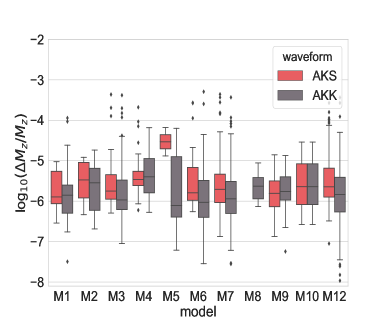
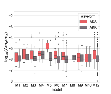
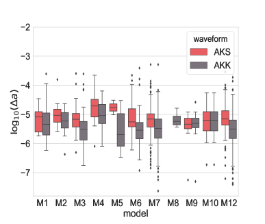
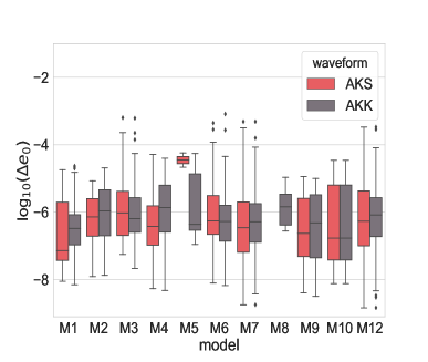
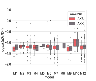
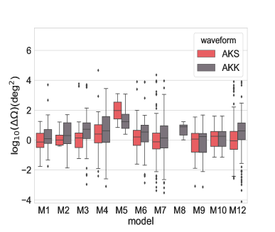
Figure 3: The parameter estimation precision for various astrophysical models, assuming AKS (red) and AKK (grey) waveforms respectively, shown in box plots. The interquartile range, or the central box, represents the middle half of all values, with the median value also shown. The points outside the box are either covered by the whiskers when the most extreme point is no further than 1.5 times the box size or extreme points are plotted individually.

As already mentioned, observation of the GW signal from EMRIs by space-based detectors may allow for testing the no-hair theorem Ryan (1995, 1997a, 1997b); Glampedakis and Babak (2006); Barack and Cutler (2007); Gair et al. (2013); Chua et al. (2018) and for revealing the possible presence of matter surrounding MBHs Barausse et al. (2007); Barausse and Rezzolla (2008); Gair et al. (2011); Yunes et al. (2011); Barausse et al. (2014, 2015). Moreover, EMRIs may permit gaining information on the mass distribution of MBHs Gair et al. (2010) and on their host stellar environments Amaro-Seoane et al. (2007), as well as on the expansion of the Universe MacLeod and Hogan (2008). All these goals, however, rely on high-precision measurements of the source parameters. In this section, we therefore investigate the parameter estimation of EMRIs with TianQin, using a FIM approach.

Among the 14 parameters introduced in Sec. II.2, one is generally mostly interested in the redshifted mass $m_{z}$ and the orbital eccentricity $e_{0}$ of the CO, the redshifted mass $M_{z}$ and the spin $a$ of the MBH, the luminosity distance to the source $D_{L}$, and the sky localization (the solid angle within which the source is located) $\Omega$. The FIM-predicted uncertainties in the estimation of these parameters are given in Fig. 3 for AKS and AKK waveforms shown in the form of box plots. The central box represents the middle half with the central line indicating the median value. The whiskers covers the most extreme points when it is shorter than 1.5 times the box size; otherwise, the more extreme points are plotted individually.

We first notice that, although the 12 models cover a wide range of different astrophysical setups, the distributions of the predicted errors are quite similar as expected from earlier studies conducted for the LISA mission Babak et al. (2017). Although notice that, for the models M8 and M11, the ratio between plunges to EMRIs is extremely high, so that the expected event rates are among the lowest, and, therefore, the detection rates can be as low as zero. Different choices of cutoff between the AKK and AKS waveforms can make a difference in the overall detectability in model M8, where we expect to detect six events assuming AKK waveform, no detection is expected when adopting AKS waveform. This leads to the difference in Figs. 3 and 4. There is also an intriguing similarity between the results of AKS and AKK, as one may have expected much better results for AKK waveforms. Indeed, for a prograde source that can be detected with both AKS and AKK waveforms, the precision of parameter estimation is certainly better with AKK waveforms, because the SNR is greater. However, there is a large portion of events that can be detected with AKK waveforms, but which do not have enough SNR when using AKS waveforms. The high precision achieved for the high SNR events is largely diluted by these relatively low SNR events. In this sense, the similarity between AKS and AKK is a demonstration of the strong link between the SNR and the precision of parameter estimation.

Figs. 3 also shows a stark difference between intrinsic and extrinsic parameters. The intrinsic parameters are those that contribute to the phase of the GWs, such as the redshifted mass $M_{z}$ and the spin $a$ of the MBH, and the redshifted mass $m_{z}$ and the orbit eccentricity $e_{0}$ of the CO. Parameters such as the luminosity distance $D_{L}$ and the sky localization $\Omega$ affect only the amplitude of the GWs, and are referred to as extrinsic. Assuming a typical observation time of $10^{8}$ s and a typical frequency of $10^{-2}$Hz, the number of wave cycles in an EMRI signal is of the order of $10^{6}$. Because of the huge number of cycles, a very slight change in the intrinsic parameters (and, hence in the phase) could change the cycle number by one, which is, in principle, detectable. Therefore, a (relative) precision of the order of $10^{-6}$ is expected for the intrinsic parameters. We indeed observe peaks roughly at this precision in Fig. 3, for all models. On the other hand, the estimation of the extrinsic parameters cannot benefit from the accumulation of a large number of wave cycles, and, therefore, the expected precision is much worse than for the intrinsic parameters.

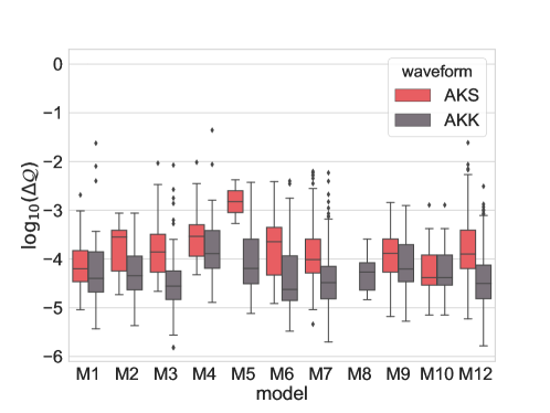
Figure 4: The parameter estimation precision for the “anomalous” quadrupole moment $\mathcal{Q}$ defined in the text, for AKS (red) and AKK (gray) waveforms, shown in box plots, with the same setting as in Fig. 3.

We have also considered the possibility of testing the no-hair theorem by measuring the multipole moments of the MBH Ryan (1997c); Barack and Cutler (2007); Cornish and Larson (2001). A Kerr black hole satisfies the no-hair theorem and has a quadruple moment $Q_{K}$ determined completely by its mass and spin: $Q_{K}=-a^{2}M^{3}$ Hansen (1974). Here, we relax the Kerr hypothesis and allow for the quadrupole moment $Q$ to deviate from the Kerr value. In Fig. 4, we present the predicted errors on the dimensionless quantity $\mathcal{Q}\equiv(Q-Q_{k})/M^{3}$, with the two distributions corresponding to the AKS and AKK waveform for the 12 models, respectively.

IV.4 TianQin in a network of detectors

The operation of TianQin inevitably leads to gaps between data or effectively lowering the duty cycle for the observation. The proposed twin constellation configuration of TQ I+II, where two identical constellations differ only by orientation, has been considered in the following consideration. The TQ II constellation would be perpendicular to both the ecliptic plane and the orbital plane of TQ. Under such a design, and adopting the nominal 3 months operation followed by 3 months break, the TQ II can be configured in a relay mode so that when the TQ starts operation exactly when the TQ II ends, there would be no gap between data and, therefore, significantly increase the duty cycle. We briefly discuss the intriguing possibility that TianQin could be observing within a network of detectors, such as TQ I+II, TQ + LISA, and TQ I+II + LISA (see Huang et al. (2020) for a detailed explanation of each of the detector networks).

In Fig. 5, we plot the expected detection rate using TQ and TQ I+II, adopting AKK waveforms. Note that, for burst signals, extending the observation time to full coverage would effectively double the detection rate. However, since EMRIs are long-lived sources, the increase in the detection rate will not scale with the duty cycle, and is shown in Fig. 5. As can be seen, detection rates could increase by a factor ranging from $\sim 2$ in model 8 up to even $\sim 3$.

A comparison of the precision of parameter estimation with TQ, TQ I+II, LISA, TQ +LISA, and TQ I+II+LISA is given in Table 2. In the calculation, we considered EMRIs with four different MBH masses log$(M/M_{\odot})=5,5.5,6,6.5$ using the same set of parameters assumed for the horizon distance calculation, with the exception of the plunge time, which is taken to be 1 yr, and the luminosity distance, which is taken to be 1 Gpc. Notice that, due to the better sensitivity in lower frequency, LISA outperforms TianQin consistently, by no more than one order of magnitude. We note that a detector network can usually improve on the precision of sky localization by more than 20 times, while for other parameters, the improvement can reach over 5 times. As a comparison among the networks of detectors, TQ+LISA is consistently better than TQ I+II, while TQ I+II + LISA is always the best.

Table 2: Parameter estimation precisions for different sources of TQ, TQ I+II, LISA, TQ+LISA and TQ I+II+LISA.

MBH mass	configuration	$\Delta{M_{z}}/M_{z}$	$\Delta{m_{z}}/m_{z}$	$\Delta{a}$	$\Delta{e_{0}}$	$\Delta{D_{L}}/D_{L}$	$\Delta\Omega$(deg2)
log$(\frac{M}{M_{\odot}})=5.0$	TQ	$2.25\times 10^{-7}$	$9.15\times 10^{-7}$	$1.46\times 10^{-7}$	$1.71\times 10^{-8}$	$2.23\times 10^{-2}$	0.31
	TQ I+II	$1.54\times 10^{-7}$	$7.3\times 10^{-7}$	$1.15\times 10^{-7}$	$1.25\times 10^{-8}$	$2.19\times 10^{-2}$	0.19
	LISA	$1.15\times 10^{-7}$	$6.76\times 10^{-7}$	$1.01\times 10^{-7}$	$0.98\times 10^{-8}$	$2.67\times 10^{-2}$	0.18
	TQ+LISA	$1.01\times 10^{-7}$	$4.86\times 10^{-7}$	$0.80\times 10^{-7}$	$0.84\times 10^{-8}$	$1.70\times 10^{-2}$	0.09
	TQ I+II+LISA	$0.91\times 10^{-7}$	$4.67\times 10^{-7}$	$0.75\times 10^{-7}$	$0.76\times 10^{-8}$	$1.69\times 10^{-2}$	0.08
log$(\frac{M}{M_{\odot}})=5.5$	TQ	$1.87\times 10^{-6}$	$1.41\times 10^{-6}$	$6.3\times 10^{-7}$	$4.09\times 10^{-7}$	$1.27\times 10^{-2}$	$1.51$
	TQ I+II	$1.23\times 10^{-6}$	$0.82\times 10^{-6}$	$5.47\times 10^{-7}$	$2.32\times 10^{-7}$	$1.24\times 10^{-2}$	0.46
	LISA	$0.97\times 10^{-6}$	$0.68\times 10^{-6}$	$5.06\times 10^{-7}$	$2.16\times 10^{-7}$	$1.15\times 10^{-2}$	0.22
	TQ+LISA	$0.72\times 10^{-6}$	$0.51\times 10^{-6}$	$3.59\times 10^{-7}$	$1.51\times 10^{-7}$	$0.85\times 10^{-2}$	$0.15$
	TQ I+II+LISA	$0.69\times 10^{-6}$	$0.49\times 10^{-6}$	$3.51\times 10^{-7}$	$1.48\times 10^{-7}$	$0.84\times 10^{-2}$	$0.14$
log$(\frac{M}{M_{\odot}})=6.0$	TQ	$6.63\times 10^{-6}$	$3.53\times 10^{-6}$	$9.66\times 10^{-7}$	$5.53\times 10^{-6}$	$9.7\times 10^{-3}$	$4.88$
	TQ I+II	$3.08\times 10^{-6}$	$1.87\times 10^{-6}$	$6.30\times 10^{-7}$	$2.55\times 10^{-6}$	$9.11\times 10^{-3}$	$1.61$
	LISA	$0.59\times 10^{-6}$	$0.44\times 10^{-6}$	$3.32\times 10^{-7}$	$0.50\times 10^{-6}$	$6.94\times 10^{-3}$	0.19
	TQ+LISA	$0.57\times 10^{-6}$	$0.40\times 10^{-6}$	$2.74\times 10^{-7}$	$0.48\times 10^{-6}$	$5.48\times 10^{-3}$	$0.16$
	TQ I+II+LISA	$0.57\times 10^{-6}$	$0.40\times 10^{-6}$	$2.72\times 10^{-7}$	$0.48\times 10^{-6}$	$5.45\times 10^{-3}$	$0.15$
log$(\frac{M}{M_{\odot}})=6.5$	TQ	$3.40\times 10^{-6}$	$5.01\times 10^{-6}$	$9.07\times 10^{-7}$	$3.38\times 10^{-6}$	$1.5\times 10^{-2}$	$11.8$
	TQ I+II	$3.04\times 10^{-6}$	$2.68\times 10^{-6}$	$8.19\times 10^{-7}$	$2.94\times 10^{-6}$	$1.46\times 10^{-2}$	$4.51$
	LISA	$0.54\times 10^{-6}$	$0.89\times 10^{-6}$	$2.74\times 10^{-7}$	$0.68\times 10^{-6}$	$0.62\times 10^{-2}$	0.49
	TQ+LISA	$0.51\times 10^{-6}$	$0.83\times 10^{-6}$	$2.59\times 10^{-7}$	$0.64\times 10^{-6}$	$0.57\times 10^{-2}$	$0.44$
	TQ I+II+LISA	$0.51\times 10^{-6}$	$0.82\times 10^{-6}$	$2.57\times 10^{-7}$	$0.64\times 10^{-6}$	$0.57\times 10^{-2}$	$0.42$

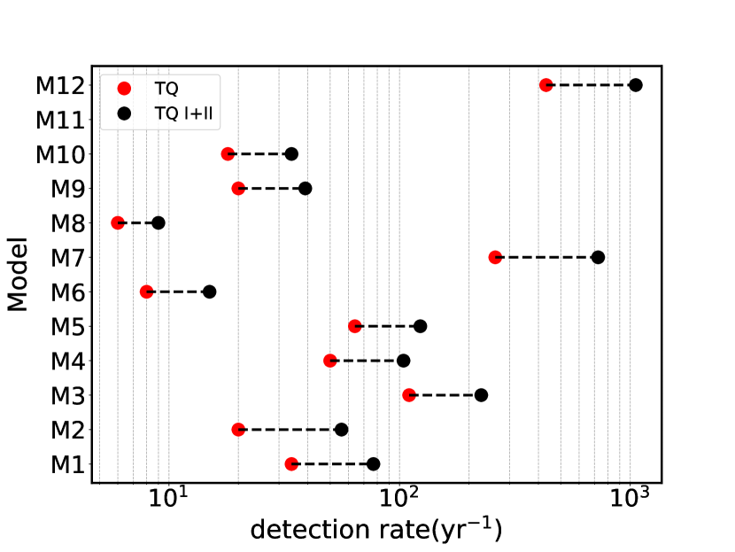
Figure 5: The expected detection rates of different models, using both the TQ (red dots) and the TQ I+II (black dots) configuration. With a logarithm scale in detection rate, the length of the dashed line segments represents the factor of improvement of detection rates.

V Summary and future work

In this work, we have performed a preliminary study of the horizon distance, detection rate and precision of parameter estimation for EMRIs with TianQin. We have employed 12 astrophysical models encapsulating a wide range of different scenarios for the underlying EMRI populations, which result in significantly different intrinsic EMRI rates (ranging from $\sim 10$ to $\sim 20000$ per year). Waveforms are described by simple analytic kludge templates.

Adopting a detection threshold of SNR=20, we find that most of the 12 astrophysical models predict that TianQin will detect dozens to thousands of EMRIs. The only model in which this is not the case (model 11) predicts that the vast majority of events should involve a CO plunging directly into the MBHs, which results in very low rates irrespective of the GW detector configuration.

As for the horizon distance, we find that EMRIs can be detected up to maximum redshifts varying from $1.6$ to $\sim 2.6$ according to what waveform model is adopted (AKS versus AKK). The MBH mass yielding the maximum horizon distance also changes from around $2\times 10^{5}~{}{\rm M}_{\odot}$ if AKS waveforms are used to around $4\times 10^{5}~{}{\rm M}_{\odot}$ for AKK waveforms. As a result, AKK waveforms also predict larger detection rates. Overall, this dependence on the waveform model highlights the need to develop fast and accurate EMRI waveforms beyond the kludge approximation.

The expected precision of the parameter estimation is calculated using the FIM method. We find that the majority of detected events can determine the intrinsic parameters to within fractional errors of $\sim 10^{-6}$, while the errors on the extrinsic parameters are much less stringent. However, the majority of detected events can still determine the relative uncertainty in the luminosity distance with $10\%$ and the uncertainty in the sky localization to the level of about $10$ deg². The precise determination of the three-dimensional location might make it possible for EMRIs to be used as standard sirens for cosmology Schutz (1986); Tamanini et al. (2016); MacLeod and Hogan (2008), although further detailed studies are needed in this direction.

We briefly consider using EMRIs to put constraints on possible deviations from the Kerr quadruple moment, and we find the uncertainty in the dimensionless parameter ${\cal Q}$ peaks at about $\Delta{\cal Q}\sim 10^{-4}$.

We also briefly consider the possible cases when TianQin is observing within a network of detectors. We find that such networks of detectors can improve the precision on sky localization by more than 20 times and the precision on other parameters as large as 5 times.