Towards Efficient Interactive Computation of
Dynamic Time Warping Distance

Abstract

The dynamic time warping (DTW) is a widely-used method that allows us to efficiently compare two time series that can vary in speed. Given two strings $A$ and $B$ of respective lengths $m$ and $n$, there is a fundamental dynamic programming algorithm that computes the DTW distance $\mathsf{dtw}(A,B)$ for $A$ and $B$ together with an optimal alignment in $\Theta(mn)$ time and space. In this paper, we tackle the problem of interactive computation of the DTW distance for dynamic strings, denoted $\mathbf{D^{2}TW}$, where character-wise edit operation (insertion, deletion, substitution) can be performed at an arbitrary position of the strings. Let $M$ and $N$ be the sizes of the run-length encoding (RLE) of $A$ and $B$, respectively. We present an algorithm for $\mathbf{D^{2}TW}$ that occupies $\Theta(mN+nM)$ space and uses $O(m+n+\#_{\mathrm{chg}})\subseteq O(mN+nM)$ time to update a compact differential representation $\mathit{DS}$ of the DP table per edit operation, where $\#_{\mathrm{chg}}$ denotes the number of cells in $\mathit{DS}$ whose values change after the edit operation. Our method is at least as efficient as the algorithm recently proposed by Froese et al. running in $\Theta(mN+nM)$ time, and is faster when $\#_{\mathrm{chg}}$ is smaller than $O(mN+nM)$ which, as our preliminary experiments suggest, is likely to be the case in the majority of instances.

1 Introduction

The dynamic time warping (DTW) is a classical and widely-used method that allows us to efficiently compare two temporal sequences or time series that can vary in speed. A fundamental dynamic programming algorithm computes the DTW distance $\mathsf{dtw}(A,B)$ for two strings $A$ and $B$ together with an optimal alignment in $\Theta(mn)$ time and space [12], where $|A|=m$ and $|B|=n$. This algorithm allows one to update the DP table $\mathit{D}$ for $\mathsf{dtw}(A,B)$ in $O(m)$ time (resp. $O(n)$ time) when a new character is appended to $B$ (resp. to $A$).

In this paper, we introduce the “dynamic” DTW problem, denoted $\mathbf{D^{2}TW}$, where character-wise edit operation (insertion, deletion, substitution) can be performed at an arbitrary position of the strings. More formally, we wish to maintain a (space-efficient) representation of $\mathit{D}$ that can dynamically be modified according to a given operation. This representation should be able to quickly answer the value of $\mathit{D}[m,n]=\mathsf{dtw}(A,B)$ upon query, together with an optimal alignment achieving $\mathsf{dtw}(A,B)$. This kind of interactive computation for (a representation of) $\mathit{D}$ can be of practical merits, e.g. when simulating stock charts, or editing musical sequences. Another example of applications of $\mathbf{D^{2}TW}$ is a sliding window version of DTW which computes $\mathsf{dtw}(A,B[j..j+d-1])$ between $A$ and every substring $B[j..j+d-1]$ of $B$ of arbitrarily fixed length $d$.

Incremental/decremental computation of a DP table is a restricted version of the aforementioned interactive computation, which allows for prepending a new character to $B$, and/or deleting the leftmost character from $B$. A number of incremental/decremental computation algorithms have been proposed for the unit-cost edit distance and weighted edit distance: Kim and Park [9] showed an incremental/decremental algorithm for the unit-cost edit distance that occupies $\Theta(mn)$ space and runs in $O(m+n)$ time per operation. Hyyrö et al. [7] proposed an algorithm for the edit distance with integer weights which uses $\Theta(mn)$ space and runs in $O(\min\{c(m+n),mn\})$ time per operation, where $c$ is the maximum weight in the cost function. This translates into $O(m+n)$ time under constant weights. Schmidt [13] gave an algorithm that uses $\Theta(mn)$ space and runs in $O(n\log m)$ time per operation for a general weighted edit distance. Hyyrö and Inenaga [5] presented a space efficient alternative to incremental/decremental unit-cost edit distance computation which runs in $O(m+n)$ time per operation but uses only $\Theta(mN+nM)$ space, where $M$ and $N$ are the sizes of run-length encoding (RLE) of $A$ and $B$, respectively. Since $M\leq m$ and $N\leq n$ always hold, the $mN+nM$ terms can be much smaller than the $mn$ term for strings that contain many long character runs. Later, Hyyrö and Inenaga [6] presented a space-efficient alternative for edit distance with integer weights, which runs in $O(\min\{c(m+n),mn\})$ time per operation and requires $\Theta(mN+nM)$ space.

Fully-dynamic interactive computation for the (weighted) edit distance was also considered: Let $j^{*}$ be the position in $B$ where the modification has been performed. For the unit cost edit distance, Hyyrö et al. [8] presented a representation of the DP table which uses $\Theta(mn)$ space and can be updated in $O(\min\{rc(m+n),mn\})$ time per operation, where $r=\min\{j^{*},n-j^{*}+1\}$ and $c$ is the maximum weight. They also showed that there exist instances that require $\Omega(\min\{rc(m+n),mn\})$ time to update their data structure per operation. Very recently, Charalampopoulos et al. [3] showed how to maintain an optimal (weighted) alignment of two fully-dynamic strings in $\tilde{O}(n\min\{\sqrt{n},c\})$ time per operation, where $m=n$.

While computing longest common subsequence (LCS) and weighted edit distance of strings of length $n$ can both be reduced to computing DTW of strings of length $O(n)$ [1, 10], a reduction to the other direction is not known. It thus seems difficult to directly apply any of the aforementioned algorithms to our $\mathbf{D^{2}TW}$ problem. Also, a conditional lower bound suggests that strongly sub-quadratic DTW algorithms are unlikely to exist [1, 2]. Thus, any method that recomputes the nav̈e DP table $\mathit{D}$ from scratch should take almost quadratic time per update.

Our contribution. This paper takes the first step towards an efficient solution to $\mathbf{D^{2}TW}$. Namely, we present an algorithm for $\mathbf{D^{2}TW}$ that occupies $\Theta(mN+nM)$ space and uses $O(m+n+\#_{\mathrm{chg}})$ time to update a compact differential representation $\mathit{DS}$ for the DP table $\mathit{D}$ per edit operation, where $\#_{\mathrm{chg}}$ denotes the number of cells in $\mathit{DS}$ whose values change after the edit operation. Since $\#_{\mathrm{chg}}=O(mN+nM)$ always holds, our method is always at least as efficient as the naïve method that recomputes the full DP table $\mathit{D}$ in $\Theta(mn)$ time, or the algorithm of Froese et al. [4] that recomputes another sparse representation of $\mathit{D}$ in $\Theta(mN+nM)$ time. While there exist worst-case instances that give $\#_{\mathrm{chg}}=\Omega(mN+nM)$, our preliminary experiments suggest that, in many cases, $\#_{\mathrm{chg}}$ can be much smaller than the size of $\mathit{DS}$ which is $\Theta(mN+nM)$.

Technically our algorithm is most related to Hyyrö et al.’s method [7, 8] and Froese et al.’s method [4], but our algorithm is not straightforward from these.

2 Preliminaries

We consider sequences (strings) of characters from an alphabet $\Sigma$ of real numbers. Let $A=a_{1},\ldots,a_{m}$ be a string consisting of $m$ characters from $\Sigma$. The run-length encoding $\mathsf{rle}(A)$ of string $A$ is a compact representation of $A$ such that each maximal run of the same characters in $A$ is represented by a pair of the character and the length of the run. More formally, let $\mathbb{N}$ denote the set of positive integers. For any non-empty string $A$, $\mathsf{rle}(A)=a_{1}^{e_{1}}\cdots a_{M}^{e_{M}}$, where $a_{I}\in\Sigma$ and $e_{I}\in\mathbb{N}$ for any $1\leq I\leq M$, and $a_{I}\neq a_{I+1}$ for any $1\leq I<M$. Each $a_{I}^{e_{I}}$ in $\mathsf{rle}(A)$ is called a (character) run, and $e_{I}$ is called the exponent of this run. The size of $\mathsf{rle}(A)$ is the number $M$ of runs in $\mathsf{rle}(A)$. E.g., for string $A=\mathtt{aacccccccbbabbbb}$ of length 16, $\mathsf{rle}(A)=\mathtt{a}^{2}\mathtt{c}^{7}\mathtt{b}^{2}\mathtt{a}^{1}\mathtt{b}^{4}$ and its size is 5.

Dynamic time warping (DTW) is a commonly used method to compare two temporal sequences that may vary in speed. Consider two strings $A=a_{1},\ldots,a_{m}$ and $B=b_{1},\ldots,b_{n}$. To formally define the DTW for $A$ and $B$, we consider an $m\times n$ grid graph $\mathcal{G}_{m,n}$ such that each vertex $(i,j)$ has (at most) three directed edges; one to the lower neighbor $(i+1,j)$ (if it exists), one to the right neighbor $(i,j+1)$ (if it exists), and one to the lower-right neighbor $(i+1,j+1)$ (if it exists). A path in $\mathcal{G}_{m,n}$ that starts from vertex $(1,1)$ and ends at vertex $(m,n)$ is called a warping path, and is denoted by a sequence $(1,1),\ldots,(i,j),\ldots,(m,n)$ of adjacent vertices. Let $\mathcal{P}_{m,n}$ be the set of all warping paths in $\mathcal{G}_{m,n}$. Note that each warping path in $\mathcal{P}_{m,n}$ corresponds to an alignment of $A$ and $B$. The DTW for strings $A$ and $B$, denoted $\mathsf{dtw}(A,B)$, is defined by $\mathsf{dtw}(A,B)=\min_{p\in\mathcal{P}_{m,n}}\sqrt{\sum_{(i,j)\in p}(a_{i}-b_{j})^{2}}$.

The fundamental $\Theta(mn)$-time and space solution for computing $\mathsf{dtw}(A,B)$, given in [12], fills an $m\times n$ dynamic programming table $\mathit{D}$ such that $\mathit{D}[i,j]=\mathsf{dtw}(A[1..i],B[1..j])^{2}$ for $1\leq i\leq m$ and $1\leq j\leq n$. Therefore, after all the cells of $\mathit{D}$ are filled, the desired result $\mathsf{dtw}(A,B)$ can be obtained by $\sqrt{\mathit{D}[m,n]}$. The value for each cell $\mathit{D}[i,j]$ is computed by the following well-known recurrence:

$$\begin{array}[]{lll}\mathit{D}[1,1]&=&(a_{1}-b_{1})^{2},\\ \mathit{D}[i,1]&=&\mathit{D}[i-1,1]+(a_{i}-b_{1})^{2}\quad\text{for }1<i\leq m,\\ \mathit{D}[1,j]&=&\mathit{D}[1,j-1]+(a_{1}-b_{j})^{2}\quad\text{for }1<j\leq n,\\ \mathit{D}[i,j]&=&\begin{array}[t]{l}\min\{\mathit{D}[i,j-1],\mathit{D}[i-1,j],\mathit{D}[i-1,j-1]\}+(a_{i}-b_{j})^{2}\\ \ \text{for $1<i\leq m$ and $1<j\leq n$.}\end{array}\end{array}$$ (1)

In the rest of this paper, we will consider the problem of maintaining a representation for $\mathit{D}$, each time one of the strings, $B$, is dynamically modified by an edit operation (i.e. single character insertion, deletion, or substitution) on an arbitrary position in $B$. We call this kind of interactive computation of $\mathsf{dtw}(A,B)$ as the dynamic DTW computation, denoted by $\mathbf{D^{2}TW}$.

Let $\mathit{B^{\prime}}$ denote the string after an edit operation is performed on $B$, and $\mathit{D^{\prime}}$ denote the dynamic programming table $\mathit{D}$ after it has been updated to correspond to $\mathsf{dtw}(A,\mathit{B^{\prime}})$. In a special case where the edit operation is performed at the right end of $B$, where we have $\mathit{B^{\prime}}=Bc$ (insertion), $\mathit{B^{\prime}}=B[1..n-1]$ (deletion) or $\mathit{B^{\prime}}=B[1..n-1]c$ (substitution) with a character $c\in\Sigma$, then $\mathit{D}$ can easily be updated to $\mathit{D^{\prime}}$ in $O(m)$ time by simply computing a single column at index $j=n$ or $j=n+1$ using recurrence (1).

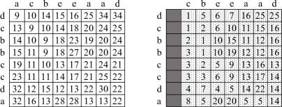
Figure 1: In this example where $A=\textrm{dcbbccda}$ and $B=\textrm{acbeeaad}$, the values of $\Theta(mn)$ cells of the DP table for $\mathsf{dtw}(A,B)$ change after the edit operation on $B$ (here, the first character $B[1]=\mathrm{a}$ of $B$ was deleted).

As in Figure 1, in the worst case, the values of $\Theta(mn)$ cells of the DP table for $\mathsf{dtw}(A,B)$ can change after an edit on $B$. The following lemma gives a stronger statement that updating $\mathit{D}$ to $\mathit{D^{\prime}}$ in our $\mathbf{D^{2}TW}$ scenario cannot be amortized:

Lemma 1

There are strings $A$, $B$ and a sequence of $k$ edits on $B$ such that $\Theta(kmn)$ cells in $\mathit{D^{\prime}}$ have different values in the corresponding cells in $\mathit{D}$.

3 Our $\mathbf{D^{2}TW}$ Algorithm based on RLE

We first explain the data structures which are used in our algorithm.

Differential representation $\mathit{DR}$ of $\mathit{D}$. The first idea of our algorithm is to use a differential representation $\mathit{DR}$ of $\mathit{D}$: Each cell of $\mathit{DR}$ contains two fields that respectively store the horizontal difference and the vertical difference, namely, $\mathit{DR}[i,j].U=\mathit{D}[i,j]-\mathit{D}[i-1,j]$ and $\mathit{DR}[i,j].L=\mathit{D}[i,j]-\mathit{D}[i,j-1]$. We let $\mathit{DR}[i,1].L=0$ for any $1\leq i\leq m$ and $\mathit{DR}[1,j].U=0$ for any $1\leq j\leq n$. The diagonal difference $\mathit{D}[i,j]-\mathit{D}[i-1,j-1]$ can easily be computed from $\mathit{DR}[i,j].U$ and $\mathit{DR}[i,j].L$ and thus is not explicitly stored in $\mathit{DR}[i,j]$.

In our algorithm we make heavy use of the following lemma:

Lemma 2

For any $1<i\leq m$,

$$\mathit{DR}[i,j].U=\begin{cases}(a_{i}-b_{1})^{2}&\mbox{if }j=1,\\ z-\mathit{DR}[i-1,j].L&\mbox{if }2\leq j\leq n,\end{cases}$$

and for any $1<j\leq n$,

$$\mathit{DR}[i,j].L=\begin{cases}(a_{1}-b_{j})^{2}&\mbox{if }i=1,\\ z-\mathit{DR}[i,j-1].U&\mbox{if }2\leq i\leq m,\end{cases}$$

where $z=\min\{\mathit{DR}[i-1,j].L,\ \mathit{DR}[i,j-1].U,\ 0\}+(a_{i}-b_{j})^{2}$.

• Proof. $\mathit{DR}[i,1].U=(a_{i}-b_{1})^{2}$ and $\mathit{DR}[1,j].L=(a_{1}-b_{j})^{2}$ are clear from recurrence (1). Now we consider $1<i\leq m$ and $1<j\leq n$, and let $d=\mathit{D}[i-1,j-1]$, $x=\mathit{DR}[i-1,j].L$, $y=\mathit{DR}[i,j-1].U$, and $d+z=D[i,j]$. Then we have $\mathit{D}[i-1,j]=d+x$ and $\mathit{D}[i,j-1]=d+y$ (see Figure 2). It follows from the definition of $\mathit{DR}$ that $\mathit{DR}[i,j].U=\mathit{D}[i,j]-\mathit{D}[i-1,j]=z-x$ and $\mathit{DR}[i,j].L=\mathit{D}[i,j]-\mathit{D}[i,j-1]=z-y$. Since $\mathit{D}[i,j]=\min\{\mathit{D}[i-1,j-1],\mathit{D}[i-1,j],\mathit{D}[i,j-1]\}+(a_{i}-b_{j})^{2}$ by recurrence (1), we obtain $d+z=\min\{d,d+x,d+y\}+(a_{i}-b_{j})^{2}$ which leads to $z=\min\{x,y,0\}+(a_{i}-b_{j})^{2}$. $\Box$

RLE-based sparse differential representation $\mathit{DS}$. The second key idea of our algorithm is to divide the dynamic programming table $\mathit{D}$ into “boxes” that are defined by intersections of maximal runs of $A$ and $B$. Note that $\mathit{D}$ contains $M\times N$ such boxes. Let $\mathsf{rle}(A)=A_{1}^{k_{1}}\dots A_{M}^{k_{M}}$ and $\mathsf{rle}(B)=B_{1}^{l_{1}}\dots B_{N}^{l_{N}}$ be the RLEs of $A$ and $B$. Let $i_{\mathrm{T}}^{I}=\sum_{i}^{I-1}{k_{i}}+1$, $i_{\mathrm{B}}^{I}=\sum_{i}^{I}{k_{i}}$, $j_{\mathrm{L}}^{J}=\sum_{j}^{J-1}{l_{j}}+1$, and $j_{\mathrm{R}}^{J}=\sum_{j}^{J}{l_{j}}$. We define a sparse table $\mathit{DS}$ for $\mathit{DR}$ that consists only of the rows and columns on the borders of the maximal runs in $A$ and $B$. Namely, $\mathit{DS}$ is a sparse table that only stores the rows $i_{\mathrm{T}}^{I},i_{\mathrm{B}}^{I}~{}(1\leq I\leq M)$ and the columns $j_{\mathrm{L}}^{J},j_{\mathrm{R}}^{J}~{}(1\leq J\leq N)$, of $\mathit{DR}$ (see Figure 3).

Figure 2: Illustration for Lemma 2 which depicts the corresponding cells of the dynamic programming table $\mathit{D}$, where $\mathit{D}[i-1,j-1]=d$, $\mathit{D}[i-1,j]=d+x$, $\mathit{D}[i,j-1]=d+y$, and $D[i,j]=d+z$. Figure 3: Illustration for $\mathit{DS}$ that consists only of the cells of $\mathit{DR}$ corresponding to the maximal run boundaries of $A$ and $B$ (white rows and columns). The gray regions that are surrounded by the box boundaries are not stored in $\mathit{DS}$.

Each row and column of $\mathit{DS}$ is implemented by a linked list as follows: each cell $\mathit{DS}[i,j]$ has four links to the upper, lower, left, and right neighbors in $\mathit{DS}$ (if these neighbors exist), plus a diagonal link to the right-lower direction. This diagonal link from $\mathit{DS}[i,j]$ points to the first cell $\mathit{DS}[i+h,j+h]$ that is reached by following the right-lower diagonal path from $\mathit{DS}[i,j]$, namely, $h\geq 0$ is the smallest integer such that $i+h=i_{\mathrm{B}}^{I}$ or $j+h=j_{\mathrm{L}}^{J}$. Clearly $\mathit{DS}$ occupies $\Theta(mN+nM)$ space. $\mathit{DS}$ can answer $\mathsf{dtw}(A,B)=\mathit{D}[m,n]$ in $O(m+n)$ time by tracing $O(m+n)$ cells of $\mathit{DS}$ from $(1,1)$ to $(m,n)$.

For each $1\leq I<M$ and $1\leq J<N$, we consider the region of $\mathit{DR}$ that is surrounded by the borders of the $I$th and $(I+1)$th runs of $A$, and the $J$th and $(J+1)$th runs of $B$. This region is called a box for $I,J$, and is denoted by $\mathcal{B}^{I,J}$. For ease of description, we will sometimes refer to a box $\mathcal{B}^{I,J}$ also in $\mathit{D}$ and $\mathit{DS}$.

3.1 Updating $\mathit{DS}$ after an edit operation

Suppose that an edit operation has been performed at position $j^{*}$ of string $B$ and let $B^{\prime}$ denote the edited string. Let $\mathit{D^{\prime}}$ denote the dynamic programming table for $\mathsf{dtw}(A,B^{\prime})$, and $\mathit{DR^{\prime}}$ the difference representation for $\mathit{D^{\prime}}$. As Figure 4 shows, the number of changed cells in $\mathit{DR^{\prime}}$ can be much smaller than that of changed cells in $\mathit{D^{\prime}}$ (see also Figure 1).

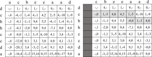
Figure 4: For the running example from Figure 1, only the gray cells have different values in the difference representations $\mathit{DR}$ (left) and $\mathit{DR^{\prime}}$ (right).

Let $\mathit{DS^{\prime}}$ denote the sparse table for $\mathit{DR^{\prime}}$. Since $\mathit{DS}$ consists only of the boundary cells, the number of changed cells in $\mathit{DS^{\prime}}$ can even be much smaller. In what follows, we show how to efficiently update $\mathit{DS}$ to $\mathit{DS^{\prime}}$.

Because the prefix $B[1..j^{*}-1]$ remains unchanged after the edit operation, for any $j<j^{*}$ we have $\mathit{DR}[i,j]=\mathit{DR^{\prime}}[i,j]$ by Lemma 2 and recurrence (1). Hence, we can restrict ourselves to the indices $j\geq j^{*}$. We define $\ell$ as a correcting offset of string indices before and after the update: $\ell=-1$ if a character has been inserted at position $j^{*}$ of $B$, $\ell=1$ if a character has been deleted from position $j^{*}$ of $B$, and $\ell=0$ otherwise. Now, for any $j\geq j^{*}$, $B^{\prime}[j]=B[j+\ell]$ and column $j$ in $\mathit{DR^{\prime}}$ corresponds to column $j+\ell$ in $\mathit{DR}$.

Let $\mathcal{B}^{I,J}$ be any box on $\mathit{DS^{\prime}}$. For the the top row $i_{\mathrm{T}}^{I}$ of $\mathcal{B}^{I,J}$, we use a linked list $\Delta_{\mathrm{T}}^{I,J}$ that stores the column indices $j$ ($j_{\mathrm{L}}^{J}\leq j\leq j_{\mathrm{R}}^{J}$) such that $\mathit{DS}[i_{\mathrm{T}}^{I},j+\ell]\neq\mathit{DS^{\prime}}[i_{\mathrm{T}}^{I},j]$, in increasing order. We also compute, in each element of the list, the value for $\mathit{D^{\prime}}[i_{\mathrm{T}}^{I},j]$ of the corresponding column index $j$. We use similar lists $\Delta_{\mathrm{B}}^{I,J}$, $\Delta_{\mathrm{L}}^{I,J}$, and $\Delta_{\mathrm{R}}^{I,J}$ for the bottom row, left column, and right column of $\mathcal{B}^{I,J}$, respectively. We compute these lists when an edit operation is performed to string $B$, and use them to update $\mathit{DS}$ to $\mathit{DS^{\prime}}$ efficiently.

Let $\#_{\mathrm{chg}}$ denote the number of cells in our sparse representation such that $\mathit{DS}[i+\ell,j]\neq\mathit{DS^{\prime}}[i,j]$. In the sequel, we prove:

Theorem 1

Our $\mathbf{D^{2}TW}$ algorithm updates $\mathit{DS}$ to $\mathit{DS^{\prime}}$ in $O(m\!+\!n\!+\!\#_{\mathrm{chg}})$ time.

Initial step. Suppose that $j^{*}$ is in the $J$th run of string $B$. Let $\mathcal{B}^{I,J}$ be any of the $M$ boxes of $\mathit{DR}$ that contain column $j^{*}$, where $j_{\mathrm{L}}^{J}\leq j^{*}\leq j_{\mathrm{R}}^{J}$. Due to Lemma 2, $(1,j^{*})$ is the only cell in the first row where we may have $\mathit{DS^{\prime}}[1,j^{*}]\neq\mathit{DS}[1,j^{*}+\ell]$. $\mathit{DS^{\prime}}[1,j^{*}]$ can be easily computed in $O(1)$ time by Lemma 2. Then, $\mathit{D^{\prime}}[1,j^{*}]$ can be computed in $O(j^{*})\subseteq O(n)$ time by tracing the first row and using $\mathit{DS^{\prime}}[1,j].L$ for increasing $j=1,\ldots,j^{*}$. The list $\Delta_{\mathrm{T}}^{I,J}$ only contains $j^{*}$ (coupled with $\mathit{D^{\prime}}[1,j^{*}]$) if $\mathit{DS^{\prime}}[1,j^{*}]\neq\mathit{DS}[1,j^{*}+\ell]$, and it is empty otherwise.

Editing string $B$ at position $j^{*}$ incurs some structural changes to $\mathit{DS}$: (a) $\mathcal{B}^{I,J}$ gets wider by one (insertion of the same character to a run), (b) $\mathcal{B}^{I,J}$ gets narrower by one (deletion of a character), (c) $\mathcal{B}^{I,J}$ is divided into $2M$ or $3M$ boxes (insertion of a different character to a run, or character substitution).

In cases (a) and (b), the diagonal links of $\mathcal{B}^{I,J}$ need to be updated. A crucial observation is that the total number of such diagonal links to update is bounded by $m$ for all the $M$ boxes $\mathcal{B}^{1,J}$, …, $\mathcal{B}^{M,J}$, since the destinations of such diagonal links are within the same column of $\mathit{DS^{\prime}}$ ($j_{\mathrm{R}}^{J}+1$ in case (a), and $j_{\mathrm{R}}^{J}-1$ in case (b)). For each box $\mathcal{B}^{I,J}$, if $j_{\mathrm{R}}^{J}-j_{\mathrm{L}}^{J}\geq i_{\mathrm{T}}^{I}-i_{\mathrm{B}}^{I}$ (i.e. $\mathcal{B}^{I,J}$ is a square or a horizontal rectangle), then we scan the top row $i_{\mathrm{T}}^{I}$ from right to left and fix the diagonal links until encountering the first cell in $i_{\mathrm{T}}^{I}$ whose diagonal link needs no updates (see Figure 6). The case with $j_{\mathrm{R}}^{J}-j_{\mathrm{L}}^{J}<i_{\mathrm{T}}^{I}-i_{\mathrm{B}}^{I}$ (i.e. $\mathcal{B}^{I,J}$ is a vertical rectangle) can be treated similarly. By the above observation, these costs for all boxes $\mathcal{B}^{I,J}$ that contain the edit position $j^{*}$ sum up to $O(m)$.

Figure 5: Case (a) of the initial step. The dashed arcs are the old diagonal links in $\mathit{DS}$, and the sold arcs are the modified diagonal links in $\mathit{DS^{\prime}}$. The gray cells depict cells $(i_{\mathrm{T}}^{I},j_{\mathrm{R}}^{J})$ and $(i_{\mathrm{B}}^{I},j_{\mathrm{R}}^{J})$. Figure 6: Case (c) of the initial step, where character substitution has been performed at position $j^{*}$. The dashed arcs are the old diagonal links in $\mathit{DS}$ from row $i_{\mathrm{T}}^{I}$ up to $j^{*}$, and the sold arcs are the modified diagonal links from new column $j^{*}$ in $\mathit{DS^{\prime}}$.

In case (a), we shift the right column $j_{\mathrm{R}}^{J}$ of $\mathit{DS}$ to the right by one position, and reuse it as the right column $j_{\mathrm{R}}^{J}+1$ of $\mathit{DS^{\prime}}$. This incurs two new cells $(i_{\mathrm{T}}^{I},j_{\mathrm{R}}^{J})$ and $(i_{\mathrm{B}}^{I},j_{\mathrm{R}}^{J})$ in $\mathit{DS^{\prime}}$ (the gray cells in Figure 6). We can compute $\mathit{DS^{\prime}}[i_{\mathrm{T}}^{I},j_{\mathrm{R}}^{J}]$ in $O(1)$ time using Lemma 2. Now consider to compute $\mathit{DS^{\prime}}[i,j_{\mathrm{R}}^{J}+1]$ for the new right column. Since this right column initially stores $\mathit{DS}[i,j_{\mathrm{R}}^{J}]$ for the old $\mathit{DS}$, using Lemma 2, we can compute $\mathit{DS^{\prime}}[i,j_{\mathrm{R}}^{J}+1]$ in increasing order of $i=1,\ldots,m$, from top to bottom, in $O(1)$ time each. We can compute $\mathit{D^{\prime}}[1,j_{\mathrm{R}}^{J}+1]$ in $O(j_{\mathrm{R}}^{J})$ time by simply scanning the first row. Then, we can compute $\mathit{D^{\prime}}[i,j_{\mathrm{R}}^{J}+1]$ for increasing $i=2,\ldots,m$, using $\mathit{DS^{\prime}}[i,j_{\mathrm{R}}^{J}+1]$, and construct $\Delta_{\mathrm{R}}^{I,J}$. This takes a total of $O(j_{\mathrm{R}}^{J}+m)\subseteq O(m+n)$ time. Finally, $\mathit{DS^{\prime}}[i_{\mathrm{B}}^{I},j_{\mathrm{R}}^{J}]$ is computed from $\mathit{D^{\prime}}[i_{\mathrm{B}}^{I},j_{\mathrm{R}}^{J}+1]$ and $\mathit{DS^{\prime}}[i_{\mathrm{B}}^{I},j_{\mathrm{R}}^{J}+1].L$ in $O(1)$ time. Case (b) can be treated similarly.

For case (c), we consider a sub-case where a character substitution was performed completely inside a run of $B$, at position $j^{*}$. This divides an existing box $\mathcal{B}^{I,J}$ into three boxes $\mathcal{B}^{I,J}$, $\mathcal{B}^{I,J+1}$, and $\mathcal{B}^{I,J+2}$. Thus, there appear three new columns $j^{*}-1$, $j^{*}$, and $j^{*}+1$ in $\mathit{DS^{\prime}}$. Then, the diagonal links for these new columns can be computed in $O(1)$ time each, by scanning row $i_{\mathrm{T}}^{I}$ from $j^{*}+1$, from right to left (see Figure 6). The $\mathit{DS^{\prime}}$ values for the cells in these new columns, as well as the $\mathit{D^{\prime}}$ values for column $j^{*}+1$, can also be computed in similar ways to cases (a) and (b). The other sub-cases of (c) can be treated similarly.

Updating cells on row $i_{\mathrm{T}}^{I}$ and column $j_{\mathrm{L}}^{J}$. In what follows, suppose that we are given a box $\mathcal{B}^{I,J}$ to the right of the edit position $j^{*}$, in which some boundary cell values may have to be updated. For ease of exposition, we will discuss the simplest case with substitution where the column indices do not change between $\mathit{DS}$ and $\mathit{DS^{\prime}}$. The cases with insertion/deletion can be treated similarly by considering the offset value $\ell$ appropriately.

Now our task is to quickly detect the boundary cells $(i,j)$ of $\mathcal{B}^{I,J}$ such that $\mathit{DS}[i,j]\neq\mathit{DS^{\prime}}[i,j]$, and to update them. We assume that the boundary cell values of the preceding boxes $\mathcal{B}^{I-1,J}$ and $\mathcal{B}^{I,J-1}$ have already been computed.

We consider how to detect the cells on the top boundary row $i_{\mathrm{T}}^{I}$ and the cells on the left boundary column $j_{\mathrm{L}}^{J}$ of box $\mathcal{B}^{I,J}$ that need to be updated, and how to update them. For this sake, we use the following lemma on the values of $\mathit{DR}$, which is immediate from Lemma 2:

Lemma 3

Let $1\leq i\leq m$ and $1\leq j\leq n$. Suppose that for any cell $(i^{\prime},j^{\prime})$ with $i^{\prime}<i$ or $j^{\prime}<j$, the value of $\mathit{DR^{\prime}}[i^{\prime},j^{\prime}]$ has already been computed. If $\mathit{DR}[i,j]\neq\mathit{DR^{\prime}}[i,j]$, then $\mathit{DR}[i,j-1].U\neq\mathit{DR}^{\prime}[i,j-1].U$ or $\mathit{DR}[i-1,j].L\neq\mathit{DR^{\prime}}[i-1,j].L$.

Intuitively, Lemma 3 states that the cell $(i,j)$ such that $\mathit{DR}[i,j]\neq\mathit{DR^{\prime}}[i,j]$ must be propagated from its left neighbor or its top neighbor. We use this lemma for updating the boundaries of each box $\mathcal{B}^{I,J}$ stored in $\mathit{DS}$. Recall that the values on the preceding row $i_{\mathrm{T}}^{I}-1=i_{\mathrm{B}}^{I-1}$ and on the preceding column $j_{\mathrm{L}}^{J}-1=j_{\mathrm{R}}^{J-1}$ have already been updated. Then, the cells on $i_{\mathrm{T}}^{I}$ and $j_{\mathrm{L}}^{J}$ of box $\mathcal{B}^{I,J}$ with $\mathit{DS}[i,j]\neq\mathit{DS^{\prime}}[i^{\prime},j^{\prime}]$ can be found in constant time each, from the lists $\Delta_{\mathrm{B}}^{I-1,J}$ and $\Delta_{\mathrm{R}}^{I,J-1}$ maintained for the preceding row $i_{\mathrm{T}}^{I}-1=i_{\mathrm{B}}^{I-1}$ and preceding column $j_{\mathrm{L}}^{J}-1=j_{\mathrm{R}}^{J-1}$, respectively.

We process column indices $\Delta_{\mathrm{B}}^{I-1,J}$ in increasing order, and suppose that we are currently processing column index $\hat{j}\in\Delta_{\mathrm{B}}^{I-1,J}$ in the bottom row $i_{\mathrm{B}}^{I-1}$ of the preceding box $\mathcal{B}^{I-1,J}$. According to the above arguments, this indicates that the cells $(i_{\mathrm{T}}^{I},j)$ in the top row $i_{\mathrm{T}}^{I}$ of $\mathcal{B}^{I,J}$ that need to be updated (i.e., $\mathit{DS}[i_{\mathrm{T}}^{I},j]\neq\mathit{DS^{\prime}}[i_{\mathrm{T}}^{I},j]$). We assume that, for any $j^{\prime}$ with $j_{\mathrm{L}}^{J}\leq j^{\prime}<\hat{j}$, the value of $\mathit{DS^{\prime}}[i_{\mathrm{T}}^{I},j^{\prime}]$ has already been computed. Also, we have maintained a partial list for $\Delta_{\mathrm{T}}^{I,J}$ where the last element of this partial list stores the largest $j^{\prime\prime}$ such that $j_{\mathrm{L}}^{J}\leq j^{\prime\prime}<\hat{j}$ and $\mathit{DS}[i_{\mathrm{T}}^{I},j^{\prime\prime}]\neq\mathit{DS^{\prime}}[i_{\mathrm{T}}^{I},j^{\prime\prime}]$, together with the value of $\mathit{D}^{\prime}[i_{\mathrm{T}}^{I},j^{\prime\prime}]$. Now it follows from Lemma 2 that both $\mathit{DS^{\prime}}[i_{\mathrm{T}}^{I},\hat{j}].U$ and $\mathit{DS^{\prime}}[i_{\mathrm{T}}^{I},\hat{j}].L$ can be respectively computed in constant time from $\mathit{DS^{\prime}}[i_{\mathrm{T}}^{I}-1,\hat{j}].L$ and $\mathit{DS^{\prime}}[i_{\mathrm{T}}^{I},\hat{j}-1].U$, and thus we can check whether $\mathit{DS}[i_{\mathrm{T}}^{I},\hat{j}]\neq\mathit{DS^{\prime}}[i_{\mathrm{T}}^{I},\hat{j}]$ in constant time as well. In case $\mathit{DS}[i_{\mathrm{T}}^{I},\hat{j}]\neq\mathit{DS^{\prime}}[i_{\mathrm{T}}^{I},\hat{j}]$, we append $\hat{j}$ to the partial list for $\Delta_{\mathrm{T}}^{I,J}$. By the definition of $\mathit{DS}$, we have $\mathit{D^{\prime}}[i_{\mathrm{T}}^{I},\hat{j}]=\mathit{D^{\prime}}[i_{\mathrm{T}}^{I}-1,\hat{j}]-\mathit{DS^{\prime}}[i_{\mathrm{T}}^{I},\hat{j}].U$. Since $\mathit{D^{\prime}}[i_{\mathrm{T}}^{I}-1,\hat{j}]=\mathit{D^{\prime}}[i_{\mathrm{B}}^{I-1},\hat{j}]$ is stored with the current column index $\hat{j}$ in the list $\Delta_{\mathrm{B}}^{I-1,J}$, $\mathit{D^{\prime}}[i_{\mathrm{T}}^{I},\hat{j}]$ can also be computed in constant time.

Suppose we have processed cell $(i_{\mathrm{T}}^{I},\hat{j})$. We perform the same procedure as above for the right-neighbor cells $(i_{\mathrm{T}}^{I},\hat{j}+p)$ with $p=1$ and increasing $p$, until encountering the first cell $(i_{\mathrm{T}}^{I},\hat{j}+p)$ such that (1) $\mathit{DS}[i_{\mathrm{T}}^{I},\hat{j}+p]=\mathit{DS^{\prime}}[i_{\mathrm{T}}^{I},\hat{j}+p]$, (2) $\hat{j}+p\in\Delta_{\mathrm{B}}^{I-1,J}$, or (3) $\hat{j}+p=j_{\mathrm{R}}^{J}+1$. In cases (1) and (2), we move on to the next element of in $\Delta_{\mathrm{B}}^{I-1,J}$, and perform the same procedure as above. We are done when we encounter case (3) or $\Delta_{\mathrm{B}}^{I-1,J}$ becomes empty. The total number of cells $(i_{\mathrm{T}}^{I},\hat{j}+p)$ for all boxes in $\mathit{DS^{\prime}}$ is bounded by $\#_{\mathrm{chg}}$.

In a similar way, we process row indices $\Delta_{\mathrm{R}}^{I,J-1}$ in increasing order, update the cells on the left column $j_{\mathrm{L}}^{J}$, and maintain another partial list for $\Delta_{\mathrm{L}}^{I,J}$.

Updating cells on row $i_{\mathrm{B}}^{I}$ and column $j_{\mathrm{R}}^{J}$. Let us consider how to detect the cells on the bottom row $i_{\mathrm{B}}^{I}$ and the cells on the right column $j_{\mathrm{R}}^{J}$ of box $\mathcal{B}^{I,J}$ that need to be updated, and how to update them.

The next lemma shows monotonicity on the values of $\mathit{D}$ inside each $\mathcal{B}^{I,J}$.

Lemma 4 ([4])

For any $(i,j)$ with $1\leq i\leq m$ and $j_{\mathrm{L}}^{J}<j\leq j_{\mathrm{R}}^{J}$, $\mathit{D}[i,j]\geq\mathit{D}[i,j-1]$. For any $(i,j)$ with $i_{\mathrm{T}}^{I}<i\leq i_{\mathrm{B}}^{I}$ and $1\leq j\leq n$, $\mathit{D}[i,j]\geq\mathit{D}[i-1,j]$.

The next corollary is immediate from Lemma 4.

Corollary 1

For any cell $(i,j)$ with $1\leq i\leq m$ and $j_{\mathrm{L}}^{J}<j\leq j_{\mathrm{R}}^{J}$, $\mathit{DR}[i,j].L\geq 0$. Also, for any cell $(i,j)$ with $i_{\mathrm{T}}^{I}<i\leq i_{\mathrm{B}}^{I}$ and $1\leq j\leq n$, $\mathit{DR}[i,j].U\geq 0$.

Now we obtain the next lemma, which is a key to our algorithm.

Lemma 5

For any cell $(i,j)$ with $i_{\mathrm{T}}^{I}+1<i\leq i_{\mathrm{B}}^{I}$ and $j_{\mathrm{L}}^{J}+1<j\leq j_{\mathrm{R}}^{J}$, $\mathit{DR}[i,j]=\mathit{DR}[i-1,j-1]$.

• Proof. By Corollary 1, $\mathit{DR}[i-1,j].L\geq 0$ and $\mathit{DR}[i,j-1].U\geq 0$ for $i_{\mathrm{T}}^{I}+1<i\leq i_{\mathrm{B}}^{I}$ and $j_{\mathrm{L}}^{J}+1<j\leq j_{\mathrm{R}}^{J}$. Thus clearly $\min\{\mathit{DR}[i-1,j].L,\mathit{DR}[i,j-1].U,0\}=0$. Therefore, for the value of $z$ in Lemma 2, we have $z=(a_{i}-b_{j})^{2}$, which leads to

  $$\mathit{DR}[i,j].U = (a_{i}-b_{j})^{2}-\mathit{DR}[i-1,j].L$$ (2)

  $$\mathit{DR}[i,j].L = (a_{i}-b_{j})^{2}-\mathit{DR}[i,j-1].U$$ (3)

  By applying equation (3) to the $\mathit{DR}[i-1,j].L$ term of equation (2), we get

  $$\mathit{DR}[i,j].U=(a_{i}-b_{j})^{2}-((a_{i-1}-b_{j})^{2}-\mathit{DR}[i-1,j-1].U).$$

  Recall that $a_{i}=a_{i-1}$, since we are considering cells in the same box $\mathcal{B}^{I,J}$. Thus $\mathit{DR}[i,j].U=\mathit{DR}[i-1,j-1].U$. By applying equation (2) to the $\mathit{DR}[i,j-1].U$ term of equation (3), we similarly obtain $\mathit{DR}[i,j].L=\mathit{DR}[i-1,j-1].L$. $\Box$

For any $i_{\mathrm{T}}^{I}+1<i\leq i_{\mathrm{B}}^{I}$ and $j_{\mathrm{L}}^{J}+1<j\leq j_{\mathrm{R}}^{J}$, let $\ell$ be the smallest positive integer that satisfies $i-\ell=i_{\mathrm{T}}^{I}+1$ or $j-\ell=j_{\mathrm{L}}^{J}+1$. By Lemma 5, for any cell $(i,j)$ on the bottom row $i_{\mathrm{B}}^{I}$ or on the right column $j_{\mathrm{R}}^{J}$, we have $\mathit{DS}[i,j]=\mathit{DR}[i-\ell,j-\ell]$ and $\mathit{DS^{\prime}}[i,j]=\mathit{DR^{\prime}}[i-\ell,j-\ell]$. This means that $\mathit{DS}[i,j]\neq\mathit{DS^{\prime}}[i,j]$ iff $\mathit{DR}[i-\ell,j-\ell]\neq\mathit{DR^{\prime}}[i-\ell,j-\ell]$. Thus, finding cells $(i,j)$ with $\mathit{DS}[i,j]\neq\mathit{DS^{\prime}}[i,j]$ on the bottom row $i_{\mathrm{B}}^{I}$ or on the right column $j_{\mathrm{R}}^{J}$ reduces to finding cells $(i^{\prime},j^{\prime})$ with $\mathit{DR}[i^{\prime},j^{\prime}]\neq\mathit{DR^{\prime}}[i^{\prime},j^{\prime}]$ on the row $i_{\mathrm{T}}^{I}+1$ or on the column $j_{\mathrm{L}}^{J}+1$. See Figure 8.

Figure 7: Diagonal propagation of $\mathit{DR}[i,j]\neq\mathit{DR^{\prime}}[i,j]$ inside box $\mathcal{B}^{I,J}$. Figure 8: Illustration for the case where $s>t$ in Lemma 6.

We have shown how to compute $\Delta_{\mathrm{T}}^{I,J}$ for the top row $i_{\mathrm{T}}^{I}$ and $\Delta_{\mathrm{L}}^{I,J}$ for the left column $j_{\mathrm{L}}^{J}$. We here explain how to use $\Delta_{\mathrm{T}}^{I,J}$ (we can use $\Delta_{\mathrm{L}}^{I,J}$ in a symmetric manner). We process column indices in $\Delta_{\mathrm{T}}^{I,J}$ in increasing order, and suppose that we are currently processing column index $\hat{j}\in\Delta_{\mathrm{T}}^{I,J}$ in the top row $i_{\mathrm{T}}^{I}$ of the current box $\mathcal{B}^{I,J}$. We check whether $\mathit{DR}[i_{\mathrm{T}}^{I}+1,\hat{j}]\neq\mathit{DR^{\prime}}[i_{\mathrm{T}}^{I}+1,\hat{j}]$. For this sake, we need to know the values of $\mathit{DR}[i_{\mathrm{T}}^{I}+1,\hat{j}]$ and $\mathit{DR^{\prime}}[i_{\mathrm{T}}^{I}+1,\hat{j}]$. Recall that, by Lemma 5, $\mathit{DR}[i_{\mathrm{T}}^{I}+1,\hat{j}]$ is equal to $\mathit{DR}[i_{\mathrm{T}}^{I}+1+h,\hat{j}+h]$ ($=\mathit{DS}[i_{\mathrm{T}}^{I}+1+h,\hat{j}+h]$) on the bottom row $i_{\mathrm{B}}^{I}$ (if $i_{\mathrm{T}}^{I}+1+h=i_{\mathrm{B}}^{I}$) or on the right column $j_{\mathrm{R}}^{J}$ (if $\hat{j}+h=j_{\mathrm{R}}^{J}$), where $h>0$. Since the cell $(i_{\mathrm{T}}^{I}+1+h,\hat{j}+h)$ can be retrieved in constant time by the diagonal link from the cell $(i_{\mathrm{T}}^{I},\hat{j}-1)$ on the top row $i_{\mathrm{T}}^{I}$, we can compute $\mathit{DR}[i_{\mathrm{T}}^{I}+1,\hat{j}]$ in constant time, applying Lemma 5 to the upper-left direction.

Computing $\mathit{DR^{\prime}}[i_{\mathrm{T}}^{I}+1,\hat{j}]$ is more involved. By Lemma 2, we can compute $\mathit{DR^{\prime}}[i_{\mathrm{T}}^{I}+1,\hat{j}]$ from $\mathit{DR^{\prime}}[i_{\mathrm{T}}^{I},\hat{j}].L$ and $\mathit{DR^{\prime}}[i_{\mathrm{T}}^{I}+1,\hat{j}-1].U$. Since $(i_{\mathrm{T}}^{I},\hat{j})$ is on the top row $i_{\mathrm{T}}^{I}$, $\mathit{DR^{\prime}}[i_{\mathrm{T}}^{I},\hat{j}].L=\mathit{DS^{\prime}}[i_{\mathrm{T}}^{I},\hat{j}].L$ has already been computed. Consider to compute $\mathit{DR^{\prime}}[i_{\mathrm{T}}^{I}+1,\hat{j}-1].U$. Since $\mathit{DR^{\prime}}[i_{\mathrm{T}}^{I}+1,\hat{j}-1].U=\mathit{D^{\prime}}[i_{\mathrm{T}}^{I}+1,\hat{j}-1]-\mathit{D^{\prime}}[i_{\mathrm{T}}^{I},\hat{j}-1]$, it suffices to compute $\mathit{D^{\prime}}[i_{\mathrm{T}}^{I},\hat{j}-1]$ and $\mathit{D^{\prime}}[i_{\mathrm{T}}^{I}+1,\hat{j}-1]$. By definition, $\mathit{D^{\prime}}[i_{\mathrm{T}}^{I},\hat{j}-1]=\mathit{D^{\prime}}[i_{\mathrm{T}}^{I},\hat{j}]-\mathit{DR^{\prime}}[i_{\mathrm{T}}^{I},\hat{j}].L$. Since $\hat{j}\in\Delta_{\mathrm{T}}^{I,J}$, we can retrieve the value of $\mathit{D^{\prime}}[i_{\mathrm{T}}^{I},\hat{j}]$ from the current element of the list $\Delta_{\mathrm{T}}^{I,J}$, in $O(1)$ time. Since $\mathit{DR^{\prime}}[i_{\mathrm{T}}^{I},\hat{j}].L=\mathit{DS^{\prime}}[i_{\mathrm{T}}^{I},\hat{j}].L$, we can compute $\mathit{D^{\prime}}[i_{\mathrm{T}}^{I},\hat{j}-1]$ in $O(1)$ time.

What remains is how to compute $\mathit{D^{\prime}}[i_{\mathrm{T}}^{I}+1,\hat{j}-1]$. We use the next lemma.

Lemma 6

For any cell $(i,j)$ with $i_{\mathrm{T}}^{I}+1<i\leq i_{\mathrm{B}}^{I}$ and $j_{\mathrm{L}}^{J}+1<j\leq j_{\mathrm{R}}^{J}$, let $s=j-j_{\mathrm{L}}^{J}$ and $t=i-i_{\mathrm{T}}^{I}$. Then,

$$\mathit{D}[i,j]=\mathit{D}[i_{\mathrm{T}}^{I}+\max\{t-s,0\},j_{\mathrm{L}}^{J}+\max\{s-t,0\}]+\min\{s,t\}\cdot(a_{i}-b_{j})^{2}.$$

• Proof. Consider the case where $s>t$. By applying Lemma 4 to recurrence (1), we obtain $\mathit{D}[i,j]=\mathit{D}[i-1,j-1]+(a_{i}-b_{j})^{2}$. Since $a_{i}=a_{i^{\prime}}$ and $b_{j}=b_{j^{\prime}}$ for $i_{\mathrm{T}}^{I}<i^{\prime}<i$ and $j_{\mathrm{L}}^{J}<j^{\prime}<j$, by repeatedly applying Lemma 4 to the above equation, we get $\mathit{D}[i,j]=\mathit{D}[i_{\mathrm{T}}^{I},j_{\mathrm{L}}^{J}+(s-t)]+t\cdot(a_{i}-b_{j})^{2}$. See also Figure 8. The case $s\leq t$ is similar and we obtain $\mathit{D}[i,j]=\mathit{D}[i_{\mathrm{T}}^{I}+(t-s),j_{\mathrm{L}}^{J}]+s\cdot(a_{i}-b_{j})^{2}$. By merging the two equations for $s>t$ and $s\leq t$, we obtain the desired equation. $\Box$

Let $k=\hat{j}-j_{\mathrm{L}}^{J}$. Since $j_{\mathrm{L}}^{J}+1<\hat{j}$, $k\geq 2$. Since $s=\hat{j}-1-j_{\mathrm{L}}^{J}=k-1$, $t=i_{\mathrm{T}}^{I}+1-i_{\mathrm{T}}^{I}=1$, and $k\geq 2$, we get $s\geq t$. Thus it follows from Lemma 6 that

$$\mathit{D^{\prime}}[i_{\mathrm{T}}^{I}+1,\hat{j}-1]\!=\!\mathit{D^{\prime}}[i_{\mathrm{T}}^{I},j_{\mathrm{L}}^{J}+(k-2)]+(A[i_{\mathrm{T}}^{I}]-B[\hat{j}])^{2}\!=\!\mathit{D^{\prime}}[i_{\mathrm{T}}^{I},\hat{j}-2]+(A[i_{\mathrm{T}}^{I}]-B[\hat{j}])^{2}.$$

Since the value $\mathit{D^{\prime}}[i_{\mathrm{T}}^{I},\hat{j}]$ is already computed and stored in the corresponding element of $\Delta_{T}^{I,J}$, we can compute, in $O(1)$ time, $\mathit{D^{\prime}}[i_{\mathrm{T}}^{I},\hat{j}-2]$ by

$$\mathit{D^{\prime}}[i_{\mathrm{T}}^{I},\hat{j}-2] = \mathit{D^{\prime}}[i_{\mathrm{T}}^{I},\hat{j}]-\mathit{DR^{\prime}}[i_{\mathrm{T}}^{I},\hat{j}].L-\mathit{DR^{\prime}}[i_{\mathrm{T}}^{I},\hat{j}-1].L$$

$$= \mathit{D^{\prime}}[i_{\mathrm{T}}^{I},\hat{j}]-\mathit{DS^{\prime}}[i_{\mathrm{T}}^{I},\hat{j}].L-\mathit{DS^{\prime}}[i_{\mathrm{T}}^{I},\hat{j}-1].L.$$

Thus, we can determine in $O(1)$ time whether $\mathit{DR}[i_{\mathrm{T}}^{I}+1,\hat{j}]\neq\mathit{DR^{\prime}}[i_{\mathrm{T}}^{I}+1,\hat{j}]$, and hence whether $\mathit{DS}[i_{\mathrm{T}}^{I}+1+h,\hat{j}+h]\neq\mathit{DS^{\prime}}[i_{\mathrm{T}}^{I}+1+h,\hat{j}+h]$.

Suppose $\mathit{DS}[i_{\mathrm{T}}^{I}+1+h,\hat{j}+h]\neq\mathit{DS^{\prime}}[i_{\mathrm{T}}^{I}+1+h,\hat{j}+h]$. Then we need to compute $\mathit{D^{\prime}}[i_{\mathrm{T}}^{I}+1+h,\hat{j}+h]$. This can be computed in constant time using Lemma 6, by $\mathit{D^{\prime}}[i_{\mathrm{T}}^{I}+1+h,\hat{j}+h]=\mathit{D^{\prime}}[i_{\mathrm{T}}^{I},\hat{j}-1]+(h+1)\cdot(A[i_{\mathrm{T}}^{I}]-B[\hat{j}])^{2}$, where $\mathit{D^{\prime}}[i_{\mathrm{T}}^{I},\hat{j}-1]=\mathit{D^{\prime}}[i_{\mathrm{T}}^{I},\hat{j}]-\mathit{DR^{\prime}}[i_{\mathrm{T}}^{I},\hat{j}].L$. We add the column index $\hat{j}+h$ to list $\Delta_{\mathrm{B}}^{I,J}$ if $i_{\mathrm{T}}^{I}+1+h=i_{\mathrm{B}}^{I}$, and/or add the row index $i_{\mathrm{T}}^{I}+1+h$ to list $\Delta_{\mathrm{R}}^{I,J}$ if $\hat{j}+h=j_{\mathrm{R}}^{J}$, together with the value of $\mathit{D^{\prime}}[i_{\mathrm{T}}^{I}+1+h,\hat{j}+h]$.

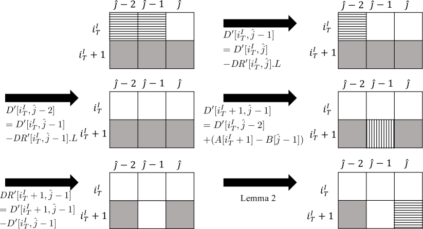
Figure 9: Illustration for the process of computing $\mathit{DR^{\prime}}[i_{\mathrm{T}}^{I}+1,\hat{j}]$. The gray cells show those for which both values of $\mathit{D^{\prime}}$ and $\mathit{DR^{\prime}}$ are unknown, the vertically striped cells show those for which only the value of $\mathit{D^{\prime}}$ is known, the horizontally striped cells show those for which only the value of $\mathit{DR^{\prime}}$ is known, and the white cells show those for which both values of $\mathit{D^{\prime}}$ and $\mathit{DR^{\prime}}$ are known. At the final step (lower-right), the desired value $\mathit{DR^{\prime}}[i_{\mathrm{T}}^{I}+1,\hat{j}]$ has been computed.

The above process of computing $\mathit{DR^{\prime}}[i_{\mathrm{T}}^{I}+1,\hat{j}]$ is illustrated in Figure 9. Suppose we have processed cell $(i_{\mathrm{T}}^{I}+1,\hat{j})$. We perform the same procedure as above for the right-neighbor cells $(i_{\mathrm{T}}^{I}+1,\hat{j}+q)$ with $q=1$ and increasing $q$, until encountering the first cell $(i_{\mathrm{T}}^{I}+1,\hat{j}+q)$ such that (1) $\mathit{DR}[i_{\mathrm{T}}^{I}+1,\hat{j}+q]=\mathit{DR^{\prime}}[i_{\mathrm{T}}^{I}+1,\hat{j}+q]$, (2) $\hat{j}+q\in\Delta_{\mathrm{T}}^{I,J}$, or (3) $\hat{j}+q=j_{\mathrm{R}}^{J}+1$. In cases (1) and (2), we remove $\hat{j}$ from $\Delta_{\mathrm{T}}^{I,J}$ and move to the next element of in $\Delta_{\mathrm{T}}^{I,J}$. We are done when we encounter case (3) or $\Delta_{\mathrm{T}}^{I,J}$ becomes empty. By Lemma 5, the total number of cells $(i_{\mathrm{T}}^{I}+1,\hat{j}+q)$ for all boxes in $\mathit{DS^{\prime}}$ is $O(\#_{\mathrm{chg}})$.

Batched updates. Our algorithm can efficiently support batched updates for insertion, deletion, substitution of a run of characters.

Theorem 2

Let $\mathit{B^{\prime}}$ be the string after a run-wise edit operation on $B$, and let $n^{\prime}=|\mathit{B^{\prime}}|$. $\mathit{DS}$ can be updated to $\mathit{DS^{\prime}}$ in $O(m+\max\{n,n^{\prime}\}+\#_{\mathrm{chg}}^{\prime})$ time where $\#_{\mathrm{chg}}^{\prime}$ denotes the number of cells where the values differ between $\mathit{DS}$ and $\mathit{DS^{\prime}}$.

Since $n^{\prime}$ is the length of the string $|\mathit{B^{\prime}}|$ after modification, $\#_{\mathrm{chg}}^{\prime}$ in Theorem 2 is bounded by $O(mN+\max\{n^{\prime},n\}M)$. Thus, we can perform a batched run-wise update on our sparse table $\mathit{DS}$ in worst-case $O(m+\max\{n,n^{\prime}\}+\#_{\mathrm{chg}}^{\prime})\subseteq O(mN+\max\{n,n^{\prime}\}M)$ time. Let $k$ be the total number of characters that are involved in a run-wise batched edit operation from $B$ to $\mathit{B^{\prime}}$ (namely, a run of $k$ characters is inserted, a run of $k$ characters is deleted, or a run of $k_{1}$ characters is substituted for a run of $k_{2}$ characters with $k=k_{1}+k_{2}$). Then a naïve $k$-time applications of Theorem 1 to the run-wise batched edit operation requires $O(k(m+n+\#_{\mathrm{chg}}))\subseteq O(k(mN+nM))$ time. Since $n^{\prime}\leq n+k$, the batched update of Theorem 2 is faster than the naïve method by a factor of $k$ whenever $k\in O(n)$. We also remark that our batched update algorithm is at least as efficient as building the sparse DP table of Froese et al.’s algorithm [4] from scratch using $\Theta(mN+\max\{n,n^{\prime}\}M)$ time and space.

3.2 Evaluation of $\#_{\mathrm{chg}}$

As was proven previously, our $\mathbf{D^{2}TW}$ algorithm works in $O(m+n+\#_{\mathrm{chg}})$ time per edit operation on one of the strings. In this subsection, we analyze how large the $\#_{\mathrm{chg}}$ would be in theory and practice. Although $\#_{\mathrm{chg}}=\Theta(mN+nM)$ in the worst case for some strings (Theorem 3), our preliminary experiments shown below suggest that $\#_{\mathrm{chg}}$ can be much smaller than $mN+nM$ in many cases.

Theorem 3

Consider strings $A=A_{1}^{k}\cdots A_{M}^{k}$ and $B=B_{1}^{l}\cdots B_{N}^{l}$ of RLE sizes $M$ and $N$, respectively, where $|A|=m=kM$ and $|B|=n=lN$. We assume lexicographical orders of characters as $A_{I-1}>A_{I}$ for $1<I\leq M$, $B_{J-1}<B_{J}$ for $1<J\leq N$, and $A_{M}>B_{N}$. If we delete $B[1]$ from $B$, then $\#_{\mathrm{chg}}=\Omega(mN+nM)$.

We have also conducted preliminary experiments to estimate practical values of $\#_{\mathrm{chg}}$, using randomly generated strings. For simplicity, we set $m=n$ and $M=N$ for all experiments. We fixed the alphabet size $|\Sigma|=26$ throughout our experiments.

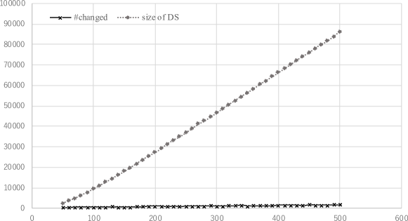
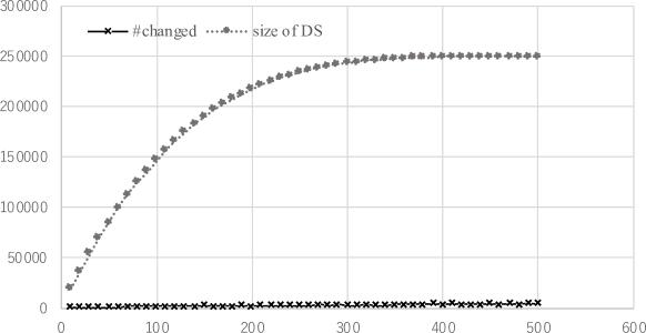
Figure 10: Comparisons of the values of $\#_{\mathrm{chg}}$ and the sizes of the sparse table $\mathit{DS}$ on two randomly generated strings $A$ and $B$. Upper: With fixed RLE size $N=M=50$ and varying lengths $n=m$ from $50$ to $500$ (horizontal axis). Lower: With fixed length $n=m=500$ and varying RLE sizes $N=M$ from $10$ to $500$ (horizontal axis).

In the first experiment, we fixed the RLE size $M=N=50$, randomly generated two strings $A$ and $B$ of varying lengths $m=n$ from $50$ to $500$, and compared the values of $\#_{\mathrm{chg}}$ and the sizes of $\mathit{DS}$. For each $m$, we randomly generated 50 pairs of strings $A$ and $B$ of length $m$ each, and took the average values for $\#_{\mathrm{chg}}$ and the sizes of $\mathit{DS}$ when $B[1]$ was deleted from $B$. In the second experiment, we fixed the string length $m=n=500$ and randomly generated two strings $A$ and $B$ of varying RLE sizes $M=N$ from $10$ to $500$. For each $M$, we randomly generated 50 pairs of strings $A$ and $B$ of RLE size $M$, and took the average values for $\#_{\mathrm{chg}}$ and the sizes of $\mathit{DS}$ when $B[1]$ was deleted from $B$. The results are shown in Figure 10. In both experiments, $\#_{\mathrm{chg}}$ is much smaller than the size of $\mathit{DS}$. It is noteworthy that even when the values of $M$ ($=N$) and $m$ ($=n$) are close, the value of $\#_{\mathrm{chg}}$ stayed very small. This suggests that our algorithm can be fast also on strings that are not RLE-compressible.

Appendix A Appendix: Omitted proofs

A.1 Proof for Theorem 3

To prove Theorem 3, we establish the following lemma.

Lemma 7

Let $\mathit{D}$ be the dynamic programming table for the above strings $A$ and $B$. Then,

$$\min\{\mathit{D}[i-1,j],\mathit{D}[i,j-1],\mathit{D}[i-1,j-1]\}=\begin{cases}\mathit{D}[i,j-1]&\mbox{if }i<j,\\ \mathit{D}[i-1,j]&\mbox{if }i>j,\\ \mathit{D}[i-1,j-1]&\mbox{if }i=j.\\ \end{cases}$$

• Proof. By recurrence (1), the argument holds for any cells $(1,j)$ and $(i,1)$, where $1\leq i\leq m$ and $1\leq j\leq n$. For any cell $(i,j)$ with $i>1$ or $j>1$, suppose that the argument holds for any $(i^{\prime},j^{\prime})$ with $i^{\prime}<i$ and $j^{\prime}<j$. We consider the five following cases:

  1. Case $i<j-1$: For the cell $(i-1,j)$, it follows from the inductive hypothesis and recurrence (1) that $\mathit{D}[i-1,j]=\mathit{D}[i-1,j-1]+(a_{i-1}-b_{j})^{2}$. Since $(a_{i-1}-b_{j})^{2}\geq 0$, $\mathit{D}[i-1,j]\geq\mathit{D}[i-1,j-1]$. Similarly, for the cells $(i-1,j-1)$ and $(i,j-1)$, $\mathit{D}[i-1,j-1]=\mathit{D}[i-1,j-2]+(a_{i-1}-b_{j-1})^{2}$ and $\mathit{D}[i,j-1]=\mathit{D}[i,j-2]+(a_{i}-b_{j-1})^{2}$. Since $a_{i-1}\geq a_{i}$, $a_{i-1}-b_{j-1}\geq a_{i}-b_{j-1}$. Because $a_{i}-b_{j-1}>0$, it holds that $(a_{i-1}-b_{j-1})^{2}\geq(a_{i}-b_{j-1})^{2}$. By the inductive hypothesis, $\mathit{D}[i-1,j-2]\geq\mathit{D}[i,j-2]$. Thus we have $\mathit{D}[i-1,j-2]+(a_{i-1}-b_{j-1})^{2}\geq\mathit{D}[i,j-2]+(a_{i}-b_{j-1})^{2}$, which implies $\mathit{D}[i-1,j-1]\geq\mathit{D}[i,j-1]$.

  2. Case $i=j-1$: Analogously to Case 1, we get $D[i-1,j]\geq D[i-1,j-1]$. For the cells $(i-1,j-1)$ and $(i,j-1)$, it follows from the inductive hypothesis and recurrence (1) that $\mathit{D}[i-1,j-1]=\mathit{D}[i-1,j-2]+(a_{i-1}-b_{j-1})^{2}$ and $\mathit{D}[i,j-1]=\mathit{D}[i-1,j-2]+(a_{i}-b_{j-1})^{2}$. Since $(a_{i-1}-b_{j-1})^{2}\geq(a_{i}-b_{j-1})^{2}$, $\mathit{D}[i-1,j-2]+(a_{i-1}-b_{j-1})^{2}\geq\mathit{D}[i-1,j-2]+(a_{i}-b_{j-1})^{2}$, which implies $\mathit{D}[i-1,j-1]\geq\mathit{D}[i,j-1]$.

  3. Case $i-1>j$: By symmetric arguments to Case 1.

  4. Case $i-1=j$: By symmetric arguments to Case 2.

  5. Case $i=j$: For the cells $(i-1,j)$ and $(i,j-1)$, by the inductive hypothesis $\min\{\mathit{D}[i-2,j],\mathit{D}[i-1,j-1],\mathit{D}[i-1,j]\}=D[i-1,j-1]$ and $\min\{\mathit{D}[i-1,j-1],\mathit{D}[i,j-2],\mathit{D}[i,j-1]\}=D[i-1,j-1]$. Thus $\mathit{D}[i-1,j]\geq\mathit{D}[i-1,j-1]$ and $\mathit{D}[i,j-1]\geq D[i-1,j-1]$.

  $\Box$

We are ready to prove Theorem 3.

• Proof. For simplicity, we assume that the column indices of $\mathit{D}$ begin with 0. In the grid graph $\mathcal{G}_{m,n}$ over $\mathit{D}$, we assign a weight $(a_{i}-b_{j})^{2}$ to each in-coming edge of cell $(i,j)$. We also consider the grid graph $\mathcal{G}_{m-1,n}$ over $\mathit{D^{\prime}}$ obtained by removing $(1,0),\ldots,(m,0)$ from $\mathcal{G}_{m,n}$.

  Consider a cell $(i,j)$ with $1<i<j$ that is on the top row of some box $\mathcal{B}^{I,J}$, namely $i=i_{\mathrm{T}}^{I}=Ik+1$ for some $1\leq I\leq M-1$. By Lemma 7, $p_{1}=(1,0),\dots,(i,i-1),\dots,(i,j)$ is the minimum weight path from $(1,0)$ to $(i,j)$. Similarly, $p^{\prime}_{1}=(1,1),\dots,(i,i),\dots,(i,j)$ is the minimum weight path from $(1,1)$ to $(i,j)$.

  For the cell $(i-1,j)$ that is the upper neighbor of $(i,j)$ and is on the bottom row of box $\mathcal{B}^{I-1,J}$, by analogous arguments to the above, $p_{2}=(1,0),\dots,(i-1,i-2),\dots,(i-1,j)$ is the minimum weight path from $(1,0)$ to $(i-1,j)$, and $p^{\prime}_{2}=(1,1),\dots,(i-1,i-1),\dots,(i-1,j)$ is the minimum weight path from $(1,1)$ to $(i-1,j)$.

  Let $p_{3}$ be the sub-path of $p_{1}$ and $p_{2}$ ending at $(i-1,i-2)$, $p_{4}$ the sub-path of $p^{\prime}_{1}$ and $p^{\prime}_{2}$ ending at $(i-1,i-1)$, $p_{5}$ the sub-path of $p_{1}$ and $p^{\prime}_{1}$ from $(i,i)$ to $(i,j)$, and $p_{6}$ the sub-path of $p_{2}$ and $p^{\prime}_{2}$ from $(i-1,i-1)$ to $(i-1,j)$. Let $e_{1}$ be the edge from $(i-1,i-2)$ to $(i,i-1)$, $e_{2}$ be the edge from $(i,i-1)$ to $(i,i)$, $e_{3}$ be the edge from $(i-1,i-2)$ to $(i-1,i-1)$, and $e_{4}$ be the edge from $(i-1,i-1)$ to $(i,i)$. See Figure 11 that depicts these paths and edges.

  

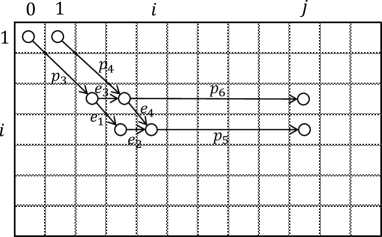
  Figure 11: Minimum weight paths to $(i,j)$ and $(i-1,j)$ over $\mathit{D}$ and $\mathit{D^{\prime}}$.

For any path $p$ in $\mathcal{G}_{m,n}$, let $\mathsf{w}(p)$ denote the total weights of edges in $p$. Now we have $\mathsf{w}(p_{1})=\mathsf{w}(p_{3})+\mathsf{w}(e_{1})+\mathsf{w}(e_{2})+\mathsf{w}(p_{5})$ and $\mathsf{w}(p^{\prime}_{1})=\mathsf{w}(p_{4})+\mathsf{w}(e_{4})+\mathsf{w}(p_{5})$. By the definition of DTW, $\mathit{D}[i,j]$ stores the cost of the minimum weight path from $(1,0)$ to $(i,j)$, and $\mathit{D^{\prime}}[i,j]$ stores the cost of the minimum weight path from $(1,1)$ to $(i,j)$. Thus $\mathit{D}[i,j]=\mathsf{w}(p_{3})+\mathsf{w}(e_{1})+\mathsf{w}(e_{2})+\mathsf{w}(p_{5})$ and $\mathit{D^{\prime}}[i,j]=\mathsf{w}(p_{4})+\mathsf{w}(e_{4})+\mathsf{w}(p_{5})$. Similarly, $\mathit{D}[i-1,j]=\mathsf{w}(p_{3})+\mathsf{w}(e_{3})+\mathsf{w}(p_{6})$ and $\mathit{D^{\prime}}[i-1,j]=\mathsf{w}(p_{4})+\mathsf{w}(p_{6})$.

Now $\mathit{DS}[i,j].U=\mathit{D}[i-1,j]-\mathit{D}[i,j]=\mathsf{w}(e_{3})+\mathsf{w}(p_{6})-(\mathsf{w}(e_{1})+\mathsf{w}(e_{2})+\mathsf{w}(p_{5}))$, and $\mathit{DS^{\prime}}[i,j].U=\mathit{D^{\prime}}[i-1,j]-\mathit{D^{\prime}}[i,j]=\mathsf{w}(p_{6})-(\mathsf{w}(e_{4})+\mathsf{w}(p_{5}))$. This leads to $\mathit{DS}[i,j].U-\mathit{DS^{\prime}}[i,j].U=\mathsf{w}(e_{3})+\mathsf{w}(e_{4})-(\mathsf{w}(e_{1})+\mathsf{w}(e_{2}))$. Recall that $\mathsf{w}(e_{2})=\mathsf{w}(e_{4})=(A[i]-B[j])^{2}$. Thus $\mathit{DS}[i,j].U-\mathit{DS^{\prime}}[i,j].U=\mathsf{w}(e_{3})-\mathsf{w}(e_{1})$. Also, because $A[i]\neq A[i-1]$, $(A[i]-B[i-1])^{2}=\mathsf{w}(e_{1})\neq\mathsf{w}(e_{3})=(A[i-1]-B[i-1])^{2}$, Consequently, $\mathit{DS}[i,j].U-\mathit{DS^{\prime}}[i,j].U\neq 0$.

Therefore, for any cell $(i,j)$ with $1<i<j$ that lies on the top row of any character run in $A$, $\mathit{DS}[i,j]\neq\mathit{DS^{\prime}}[i,j]$. Since each top row $i_{\mathrm{T}}^{I}=Ik+1$ $(1\leq I\leq M-1)$ contains $n-(Ik+1)$ such cells, and since $n=kM$, there are $\sum_{I=1}^{M-1}{(n-(Ik+1))}=n(M-1)-k((M-1)M)/2-(M-1)=(n-2)(M-1)/2$ such cells for top rows $I=1,\ldots,M-1$. Symmetric arguments show that there are $\sum_{J=1}^{N-1}{(m-(Jl+1))}=(m-2)(N-1)/2$ cells with $\mathit{DS}[i,j]\neq\mathit{DS^{\prime}}[i,j]$ for left rows $J=1,\ldots,N-1$. Thus, $\#_{\mathrm{chg}}\geq((n-2)(M-1)+(m-2)(N-1))/2\in\Omega(mN+nM)$. $\Box$

A.2 Proof for Lemma 1

• Proof. The lemma can be shown in a similar manner to the proof for Theorem 3 above. In so doing, we set $M=n$ and $N=n$ in the strings $A$ and $B$ of Section 3.2, and consider strings $A$ and $B$ such that $A[i-1]>A[i]$ for $1<i\leq m$ and $B[j-1]<B[j]$ for $1<j\leq n$, and $A[m]>B[n]$. Since deleting the leftmost character $B[1]$ of $B$ is symmetric to appending a new character $b_{1}$ to $B$ such that $b_{1}<B[1]$, we get $\Omega(mn)$ lower bound for the number of cells where $D[i,j]\neq\mathit{D^{\prime}}[i,j]$ per appended character. If we repeat this by recursively appending $k$ new characters $b_{i}$ such that $b_{i}<b_{i-1}<\cdots<B[1]$ for $i=2,\ldots,k$, we get $\Omega(mn)$ lower bound for the number of cells where $D[i,j]\neq\mathit{D^{\prime}}[i,j]$ for each $b_{i}$. Hence there are a total of $\Theta(kmn)$ cells in $\mathit{D^{\prime}}$ that differ from the corresponding cells in $\mathit{D}$, for $k$ edit operations on $B$. $\Box$

References

- [1] A. Abboud, A. Backurs, and V. V. Williams. Tight hardness results for LCS and other sequence similarity measures. In FOCS 2015, pages 59–78, 2015.
- [2] K. Bringmann and M. Künnemann. Quadratic conditional lower bounds for string problems and dynamic time warping. In FOCS 2015, pages 79–97, 2015.
- [3] P. Charalampopoulos, T. Kociumaka, and S. Mozes. Dynamic string alignment. In CPM 2020, pages 9:1–9:13, 2020.
- [4] V. Froese, B. J. Jain, M. Rymar, and M. Weller. Fast exact dynamic time warping on run-length encoded time series. CoRR, abs/1903.03003, 2020.
- [5] H. Hyyrö and S. Inenaga. Compacting a dynamic edit distance table by RLE compression. In SOFSEM 2016, pages 302–313, 2016.
- [6] H. Hyyrö and S. Inenaga. Dynamic RLE-compressed edit distance tables under general weighted cost functions. Int. J. Found. Comput. Sci., 29(4):623–645, 2018.
- [7] H. Hyyrö, K. Narisawa, and S. Inenaga. Dynamic edit distance table under a general weighted cost function. In SOFSEM 2010, pages 515–527, 2010.
- [8] H. Hyyrö, K. Narisawa, and S. Inenaga. Dynamic edit distance table under a general weighted cost function. J. Disc. Algo., 34:2–17, 2015.
- [9] S.-R. Kim and K. Park. A dynamic edit distance table. J. Disc. Algo., 2:302–312, 2004.
- [10] W. Kuszmaul. Dynamic time warping in strongly subquadratic time: Algorithms for the low-distance regime and approximate evaluation. In ICALP 2019, pages 80:1–80:15, 2019.
- [11] A. Nishi, Y. Nakashima, S. Inenaga, H. Bannai, and M. Takeda. Towards efficient interactive computation of dynamic time warping distance. CoRR, abs/2005.08190, 2020.
- [12] H. Sakoe and S. Chiba. Dynamic programming algorithm optimization for spoken word recognition. IEEE Transactions on Acoustics, Speech, and Signal Processing, 26(1):43–49, 1978.
- [13] J. P. Schmidt. All highest scoring paths in weighted grid graphs and their application in finding all approximate repeats in strings. SIAM J. Comp., 27(4):972–992, 1998.